An Analytical Two-Dimensional Linearized Droplet Shape Model for Combined Tangential and Normal Body Forces

Abstract

In view of emerging research on forced wetting under complex applied forces, a simple model for a droplet shape evolution is developed here. In particular, the model refers to droplet spreading under quasisteady conditions. The corresponding linearized two-dimensional Young–Laplace equation is solved analytically resulting in a system of two equations that relates the droplet shape features to each other. Despite its simplicity, the final model produces a wealth of droplet behaviors when combined with the physical requirement that the contact angle should be within a particular range of values. Indicative results of the droplet behavior under several forces scenarios are examined here exhibiting why the present model is useful for designing experimental campaigns on forced spreading.

1. Introduction

Wetting behavior of liquids on solid surfaces affects the process effectiveness in several unit processes of chemical technology (e.g., condensation [1], flotation [2]). Whereas, on a small-size scale, wetting behavior is completely determined by molecular forces, the situation is different for larger-size scales where body and surface forces are of importance [3]. The transition size from the one to the other dependence is affected by the magnitude of external forces and is typically of the order of hundreds of micrometers for common forces met in practice (e.g., induced by acceleration fields with values of up to tens of g). Spreading is a term typically employed to describe the partial motion of a droplet contact line under the influence of external forces whereas the term sliding refers to the motion of the whole droplet. The transition from spreading to sliding has been an evergreen research topic over the years. The spreading behavior in case of a slowly varying external body force (compared to the droplet hydrodynamic time scale) depends only on the external force magnitude and on the molecular forces (as expressed by surface tension and contact angles). The experimental campaigns on the subject until recently have been restricted to either tangential or normal forces and to specific combinations of the two forces arising by tilting droplets in the earth gravitational field [4,5,6]. Only recently have more complex combinations and scenarios of applied forces have been tested [7,8,9].

The exploitation of these data (and also additional data of this type to emerge in the literature in the future) requires employment of corresponding mathematical models. The physics of the particular problem is well-founded and the basic mathematical tool for the droplet shape is the three dimensional Young–Laplace equation [10]. Whereas the prediction of the droplet shape for a given contact line contour is well established, the prediction of the contact line evolution during forced wetting is rather based on empirical arguments. An extensive analysis on the subject can be found in [11]. The droplet equilibrium shape can be found using global energy minimization approaches (e.g., Surface Evolver) [12], finite element solvers [13], perturbation expansion methods (only for small deformations) [14], intelligent dimensionality reduction approaches (only for specific contact line shapes) [15,16] and boundary collocation (only for the linearized problem and omniphilic surfaces) [11]. The computation effort ratio from the first to the last method is of the order of millions.

According to [17], there are two limiting categories of models: the first attempts to include as many details as possible at the cost of complexity and specificity, whereas the second attempts to integrate general features and behaviors in the simplest possible way. Here, a model of the second type is developed for the wetting behavior of droplets on omniphilic surfaces (i.e., contact angle smaller than 90°) under combined evolving tangential and normal body forces. The model is a two-dimensional linearized one and is the only one that admits analytical solution. In the following section, the solution of the model is described in detail. Then it is applied to demonstrate several interesting results on the droplet behavior for some scenarios of combined applied forces.

2. Theoretical Analysis

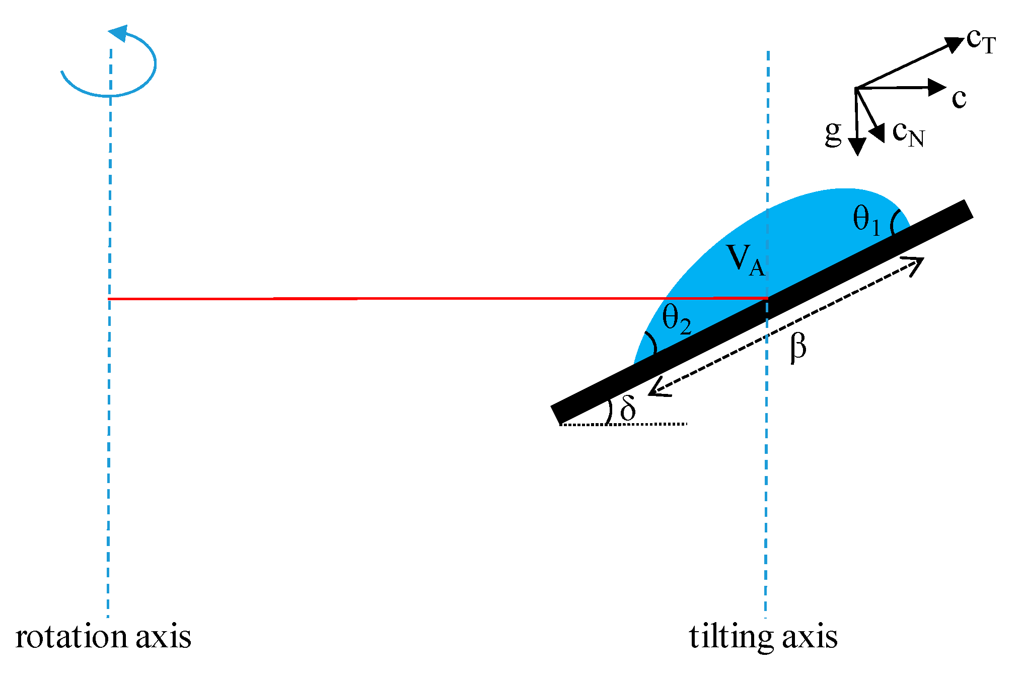
Up to now, experimental studies on forced spreading refer to one of two effects: either to simple tilting plates or to centrifugal devices with varying tangential force applied to a droplet lying horizontally. Hence, theoretical studies also refer to similar conditions [4,5,6]. The generalized simultaneous variation of both effects requires new theoretical analysis. Earlier [18], an oversimplified model for the drop shape was introduced. It is based on the combination of a two-dimensional (planar) geometry and linearization of the Young–Laplace equation. Such a model is expected to give only qualitative information but it has the major advantage that it permits analytical solution retaining the essential physics of the process. In that earlier work, the model has been developed and results are presented for the case of only normal or only tangential force. Here, it is expanded for arbitrary variation of both forces and results are presented for both idealized and realistic variation scenarios. The reference set up considered for the theoretical analysis consists of a droplet lying on a plate which can be rotated and tilted simultaneously, as displayed in Figure 1. The ratio of droplet size to the distance from the rotation axis is so small that the exercised body force can be assumed uniform along the droplet.

Let us denote as f(x) the shape of the droplet, σ the liquid surface tension, ρ the liquid density and C_N, C_T the global (rotational plus gravitational) normal and tangential acceleration field values, respectively. The problem has not a unique intrinsic characteristic length (in general the droplet length is unknown) so usually the capillary length is used for non-dimensionalization [19]. Recently, the problem of defining a relevant Bond number is reconsidered revealing that at least five different characteristic lengths have been employed in the literature [20]. Even in the case of a known droplet radius, its use as characteristic length does not usually offer a meaningful non-dimensionalization. For example, in the case of normal force, the droplet height and not the droplet length is responsible for the effect of gravity. The new Bond number proposed in [21] depends on force direction. For the above reasons it is found more convenient to use as characteristic length a size scale simply relevant to the actual one, instead of using the capillary length or a droplet dimension. This choice in the present work is L = 1 mm. The major advantage of this definition of Bond number is that it is a property of the external forcing field and is not related to the specific droplet studied.

The dimensionless linearized (i.e., exact in the limit df/dx << 1) two-dimensional Young–Laplace equation for simultaneous normal and tangential forces, with the corresponding Bond numbers denoted as Bo_N (=ρC_NL²/σ) and Bo_T (=ρC_TL²/σ), takes the form (f and x are normalized by L):

$$\frac{{\partial }^2\mathrm{f}}{\partial {\mathrm{x}}^2}=-\mathrm{G}-\mathrm{B}{\mathrm{o}}_{\mathrm{T}}\mathrm{x}+\mathrm{B}{\mathrm{o}}_{\mathrm{N}}\mathrm{f}$$

(1)

The parameter G is related to the pressure in the droplet and it is an unknown quantity which has to be found from the solution of the mathematical problem. Let us call β the contact line length of the droplet. The origin of the x axis (x = 0) is designated to the rear (with respect to tangential acceleration direction) droplet edge. The following conditions must be fulfilled by the function f:

f(0) = 0

(2)

f(β) = 0

(3)

$${\left(\frac{\partial \mathrm{f}}{\partial \mathrm{x}}\right)}_{\mathrm{x}=\mathsf{\beta }}=-\tan ({\mathsf{\theta }}_1)$$

(4)

$${\left(\frac{\partial \mathrm{f}}{\partial \mathrm{x}}\right)}_{\mathrm{x}=0}=\tan ({\mathsf{\theta }}_2)$$

(5)

$${\mathrm{V}}_{\mathrm{A}}={\displaystyle \underset{0}{\overset{\mathsf{\beta }}{\int }}\mathrm{fdx}}$$

(6)

where θ₁ and θ₂ are the front and rear contact angle, respectively, and V_A is the area under the droplet profile (i.e., two-dimensional “volume” or alternatively volume per unit length in the third dimension).

The general solution of the equation can be found as the sum of the homogeneous solution and of a particular solution:

$$\mathrm{f}={\mathrm{c}}_1{\mathrm{e}}^{-\mathrm{Ax}}+{\mathrm{c}}_2{\mathrm{e}}^{\mathrm{Ax}}+\mathrm{Ex}+\frac{\mathrm{G}}{\mathrm{B}{\mathrm{o}}_{\mathrm{N}}}$$

(7)

where the symbols A = (Bo_N)^0.5 and E = Bo_T/Bo_N have been introduced for clarity of presentation. Substitution of Equation (7) in Equations (2)–(4) leads to the following Equations (8)–(10), respectively:

$${\mathrm{c}}_1+{\mathrm{c}}_2+\frac{\mathrm{G}}{\mathrm{B}{\mathrm{o}}_{\mathrm{N}}}=0$$

(8)

$${\mathrm{c}}_1{\mathrm{e}}^{-\mathrm{A}\mathsf{\beta }}+{\mathrm{c}}_2{\mathrm{e}}^{\mathrm{A}\mathsf{\beta }}+\mathrm{E}\mathsf{\beta }+\frac{\mathrm{G}}{\mathrm{B}{\mathrm{o}}_{\mathrm{N}}}=0$$

(9)

$$-\mathrm{A}{\mathrm{c}}_1{\mathrm{e}}^{-\mathrm{A}\mathsf{\beta }}+\mathrm{A}{\mathrm{c}}_2{\mathrm{e}}^{\mathrm{A}\mathsf{\beta }}+\mathrm{E}=-\tan ({\mathsf{\theta }}_1)$$

(10)

Eliminating G between Equations (8) and (9) leads to:

$${\mathrm{c}}_1({\mathrm{e}}^{-\mathrm{A}\mathsf{\beta }}-1)+{\mathrm{c}}_2({\mathrm{e}}^{\mathrm{A}\mathsf{\beta }}-1)=-\mathrm{E}\mathsf{\beta }$$

(11)

The Equations (10) and (11) constitute a linear system for c₁ and c₂ which can be solved to yield:

$${\mathrm{c}}_1=\frac{-\mathrm{E}\mathsf{\beta }\mathrm{A}{\mathrm{e}}^{\mathrm{A}\mathsf{\beta }}+(\tan ({\mathsf{\theta }}_1)-\mathrm{E})({\mathrm{e}}^{\mathrm{A}\mathsf{\beta }}-1)}{\mathrm{A}(2-{\mathrm{e}}^{\mathrm{A}\mathsf{\beta }}-{\mathrm{e}}^{-\mathrm{A}\mathsf{\beta }})}$$

(12)

$${\mathrm{c}}_2=-\frac{({\mathrm{e}}^{-\mathrm{A}\mathsf{\beta }}-1)(\tan ({\mathsf{\theta }}_1)-\mathrm{E})+\mathrm{AE}\mathsf{\beta }{\mathrm{e}}^{-\mathrm{A}\mathsf{\beta }}}{\mathrm{A}(2-{\mathrm{e}}^{\mathrm{A}\mathsf{\beta }}-{\mathrm{e}}^{-\mathrm{A}\mathsf{\beta }})}$$

(13)

Finally, substituting Equation (7) in (6) and eliminating G using Equation (8) leads to the following compatibility condition:

$${\mathrm{V}}_{\mathrm{A}}=-\frac{{\mathrm{c}}_1}{\mathrm{A}}({\mathrm{e}}^{-\mathrm{A}\mathsf{\beta }}-1)+\frac{{\mathrm{c}}_2}{\mathrm{A}}({\mathrm{e}}^{\mathrm{A}\mathsf{\beta }}-1)+\mathrm{E}\frac{{\mathsf{\beta }}^2}{2}-({\mathrm{c}}_1+{\mathrm{c}}_2)\mathsf{\beta }$$

(14)

The above system of equations can be explicitly solved for θ₁ to give:

$${\mathsf{\theta }}_1={\tan }^{-1}(\frac{{\mathrm{V}}_{\mathrm{A}}-{\mathrm{N}}_1[(1-{\mathrm{e}}^{-\mathrm{A}\mathsf{\beta }})/\mathrm{A}-\mathsf{\beta }]-{\mathrm{N}}_2[({\mathrm{e}}^{\mathrm{A}\mathsf{\beta }}-1)/\mathrm{A}-\mathsf{\beta }]-\mathrm{E}{\mathsf{\beta }}^2/2}{{\mathrm{M}}_1[(1-{\mathrm{e}}^{-\mathrm{A}\mathsf{\beta }})/\mathrm{A}-\mathsf{\beta }]+{\mathrm{M}}_2[({\mathrm{e}}^{\mathrm{A}\mathsf{\beta }}-1)/\mathrm{A}-\mathsf{\beta }]})$$

(15)

where

$${\mathrm{M}}_1=\frac{{\mathrm{e}}^{\mathrm{A}\mathsf{\beta }}-1}{\mathrm{A}(2-{\mathrm{e}}^{\mathrm{A}\mathsf{\beta }}-{\mathrm{e}}^{-\mathrm{A}\mathsf{\beta }})}$$

$${\mathrm{N}}_1=\frac{-\mathrm{E}\mathsf{\beta }\mathrm{A}{\mathrm{e}}^{\mathrm{A}\mathsf{\beta }}-\mathrm{E}({\mathrm{e}}^{\mathrm{A}\mathsf{\beta }}-1)}{\mathrm{A}(2-{\mathrm{e}}^{\mathrm{A}\mathsf{\beta }}-{\mathrm{e}}^{-\mathrm{A}\mathsf{\beta }})}$$

$${\mathrm{M}}_2=\frac{-{\mathrm{e}}^{-\mathrm{A}\mathsf{\beta }}+1}{\mathrm{A}(2-{\mathrm{e}}^{\mathrm{A}\mathsf{\beta }}-{\mathrm{e}}^{-\mathrm{A}\mathsf{\beta }})}$$

$${\mathrm{N}}_2=\frac{\mathrm{E}({\mathrm{e}}^{-\mathrm{A}\mathsf{\beta }}-1)-\mathrm{AE}\mathsf{\beta }{\mathrm{e}}^{-\mathrm{A}\mathsf{\beta }}}{\mathrm{A}(2-{\mathrm{e}}^{\mathrm{A}\mathsf{\beta }}-{\mathrm{e}}^{-\mathrm{A}\mathsf{\beta }})}$$

The angle θ₂ can be found from the condition (5) as:

$${\mathsf{\theta }}_2={\tan }^{-1}(-\mathrm{A}{\mathrm{c}}_1+\mathrm{A}{\mathrm{c}}_2+\mathrm{E})$$

(16)

Equation (15) relates θ₁ το V_A, β and Equation (16) relates θ₂ το θ₁, β. In any case, if two of the above four variables are known, the other two can be found from these equations. A partial validation of the analytical model arises as follows: The following compatibility conditions were previously found [19] in case of only a tangential force applied:

$${\mathrm{V}}_{\mathrm{A}}=-\mathrm{B}{\mathrm{o}}_{\mathrm{T}}\frac{{\mathsf{\beta }}^4}{24}-\frac{{\mathsf{\beta }}^3}{6}(\frac{2\tan ({\mathsf{\theta }}_1)}{\mathsf{\beta }}-\frac{2}{3}\mathrm{B}{\mathrm{o}}_{\mathrm{T}}\mathsf{\beta })+\frac{{\mathsf{\beta }}^2}{2}(\tan ({\mathsf{\theta }}_1)-\mathrm{B}{\mathrm{o}}_{\mathrm{T}}\frac{{\mathsf{\beta }}^2}{6})$$

(17)

$${\mathsf{\theta }}_2={\tan }^{-1}(\tan ({\mathsf{\theta }}_1)-\mathrm{B}{\mathrm{o}}_{\mathrm{T}}{\mathsf{\beta }}^2/6)$$

(18)

By putting θ₁ and θ₂ equal to the advancing θ_a and the receding θ_r angle, respectively, the droplet is exactly at the critical condition for the onset of sliding so Bo_T should take its critical value Bo_Tc. Eliminating β from the above equations leads after some algebra to the relation:

$${\mathrm{V}}_{\mathrm{A}}\mathrm{B}{\mathrm{o}}_{\mathrm{T}\mathrm{c}}=-\frac{1}{2}{(\tan ({\mathsf{\theta }}_{\mathrm{a}})-\tan ({\mathsf{\theta }}_{\mathrm{r}}))}^2+\tan ({\mathsf{\theta }}_{\mathrm{a}})(\tan ({\mathsf{\theta }}_{\mathrm{a}})-\tan ({\mathsf{\theta }}_{\mathrm{r}}))$$

(19)

Expanding the trigonometric terms to a Taylor series and keeping the first terms (valid in the limit of small angles) results in:

$${\mathrm{V}}_{\mathrm{A}}\mathrm{B}{\mathrm{o}}_{\mathrm{T}\mathrm{c}}=\frac{1}{2}({\mathsf{\theta }}_{\mathrm{a}}^2-{\mathsf{\theta }}_{\mathrm{r}}^2)$$

(20)

This equation is exactly the same with the one taken by expanding the well-known sliding condition [7]:

$${\mathrm{V}}_{\mathrm{A}}\mathrm{B}{\mathrm{o}}_{\mathrm{T}\mathrm{c}}=\cos ({\mathsf{\theta }}_{\mathrm{r}})-\cos ({\mathsf{\theta }}_{\mathrm{a}})$$

in Taylor series for small angles.

It is noted that above conditions have no droplet size dependence of the critical sliding force. This dependence appears when the area V_A is assumed to be the ratio of the droplet volume to droplet width in order to account for the third dimension.

3. Indicative Model Results and Discussion

In general, the literature work associates the motion of the rear droplet edge with sliding which is true for past experimental procedures by earlier researchers. Nevertheless, this is not true in the present case of a general force variation in which the rear droplet edge motion can be due to normal force reduction occurring simultaneously with a tangential force increase. The cases of only one force component examined before [18] are based on the existence of a fixed point in the physical space (droplet center for normal force and rear contact line edge for tangential force). Therefore, the combination of forces leaves us with no fixed point in space (as is the case when a single force component increases). Let us assume that there is a valid droplet configuration with parameters β_o, θ_1o, θ_2o and the forces suddenly change to new values of Βο_Ν, Βο_Τ. The procedure of droplet shape variation is in general non-reversible and non-conservative so the exact trajectory Bo_N-Bo_T must be considered (i.e., there is no way to find directly what happens at the final conditions since the droplet evolution is history depended). In particular, the non-reversibility comes for setting limits θ_a and θ_r to the angle values (however, as far as the angles remain in-between the limiting values θ_a and θ_r, reversibility holds). The trajectory Bo_N, Bo_T must be followed by considering (infinitely small in theory but very small in calculations) small variation steps.

At the first step, Equation (15) is employed for calculation of θ₁ setting β = β_ο. Then, θ₂ is computed from Equation (16). In case of θ_r ≤ θ₁, θ₂ ≤ θ_a, the new droplet configuration is acceptable. If one of the angles overrides θ_a, then the exact point (force values) at which this angle takes the value θ_a must be found. For this, Equation (15) is solved for θ = θ_a having β as unknown. A similar procedure is followed if an angle becomes smaller than θ_r. The point with θ = θ_r must be found and then Equations (15) and (16) are solved for β. In general, the system of Equations (15) and (16) admits as input β or θ₁ or θ₂ and returns as output values of θ₁, θ₂ or β, θ₂ or β, θ₁, respectively. The above procedure is repeated for each step along the Bo_T–Bo_N trajectory. Of particular interest is the handling of the motion in the physical space. If a contact angle (or both) has the value θ_a or θ_r then the variation of β (positive for value θ_a, negative for value θ_r) is assigned to the motion of the corresponding contact line edge (or to both contact line edges in equal parts).

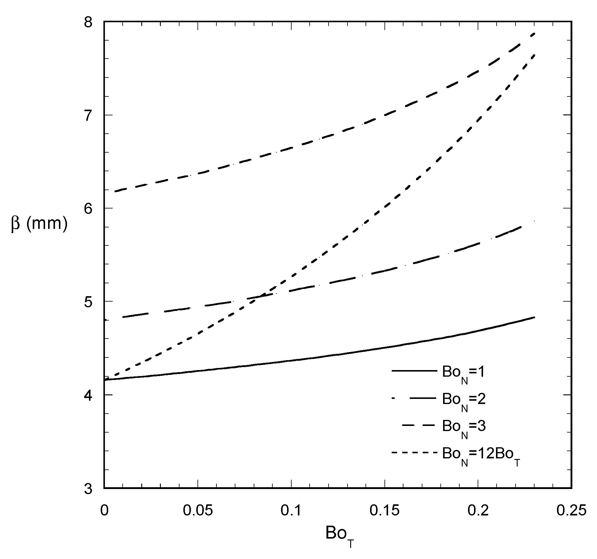
Let us first present what are the predictions of the model for some simple scenarios regarding the two forces. The case of a droplet with V_A = 5 mm², θ_a = 60° and θ_r = 40° with an increasing tangential force is examined. This case has been previously studied for zero normal force [18], so the effect of non-zero normal force is examined here. It is found that the main effect of the normal force is just to elongate the droplet with a negligible effect to the shape at the two edges. The normal force does not influence the critical Bond number Bo_Tc and, thus, the critical detachment force which is compatible to the independency of force from the droplet size according to the present model (see Equation (19)). It is reminded that this independency refers only to two dimensions (extension to the third dimension leads to the proportionality of critical force to the droplet size appearing in the well-known Furmidge equation). The Bo_N is expected to affect the critical force for sliding in three dimensions through the droplet width dependence. Figure 2 shows the increase of droplet length as Bo_T increases for an initial angle θ₀ equal to the advancing one. The evolution of the droplet profiles is quite similar to those for zero normal force [18]. In addition, introducing an oscillation of the tangential force (i.e., Bo_T varies periodically between 0 and Bo_Tc), a similar periodic behavior of droplet shape is taken independently of the normal force. In particular, after the initial transient the droplet shape retains its length (taken at Bo_Tc) and its two angles θ₁ and θ₂ oscillate following certain curves already found for Bo_N = 0 in a previous study (e.g., see [18] for details).

A more interesting scenario is the simultaneous increase of both force components (in the case of absence of gravity it corresponds to increasing the rotation speed at a fixed tilting angle). Considering exactly the same set of parameters as for a constant normal force plus the relation of Bo_N = 12 Bo_T, very interesting results are obtained. At the starting transient the droplet length increases crossing the lines of constant Bo_N (Figure 2). Under the particular conditions of the transient, a function β(Βο_Ν,Βο_Τ) can be constructed which can give directly β for arbitrary Bo_N–Bo_T trajectory. The idea behind the proposed scenarios is not the direct imitation of practical situations but the allowance to understand better the droplet shape evolution process in order to create models for any practical situation.

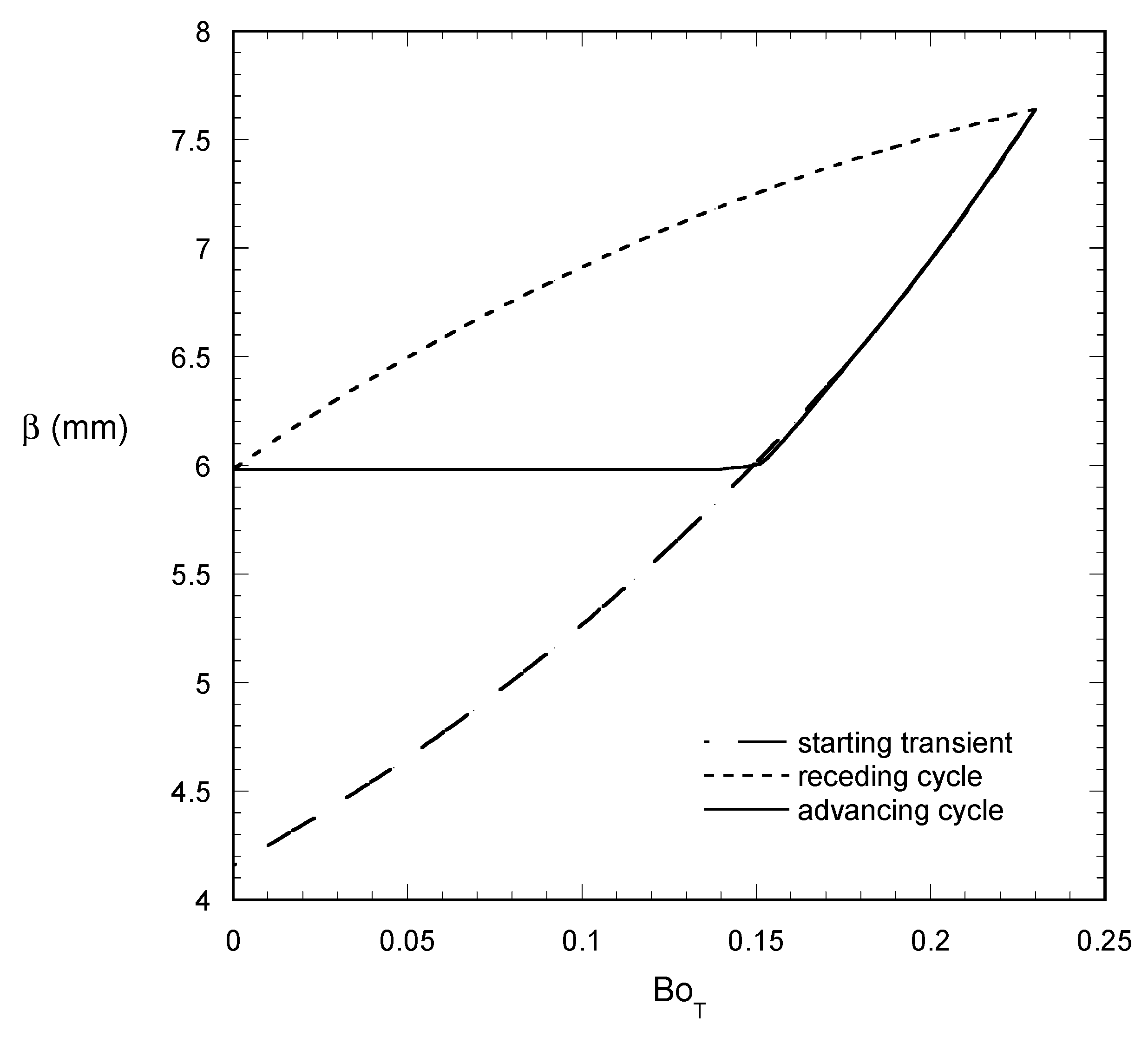
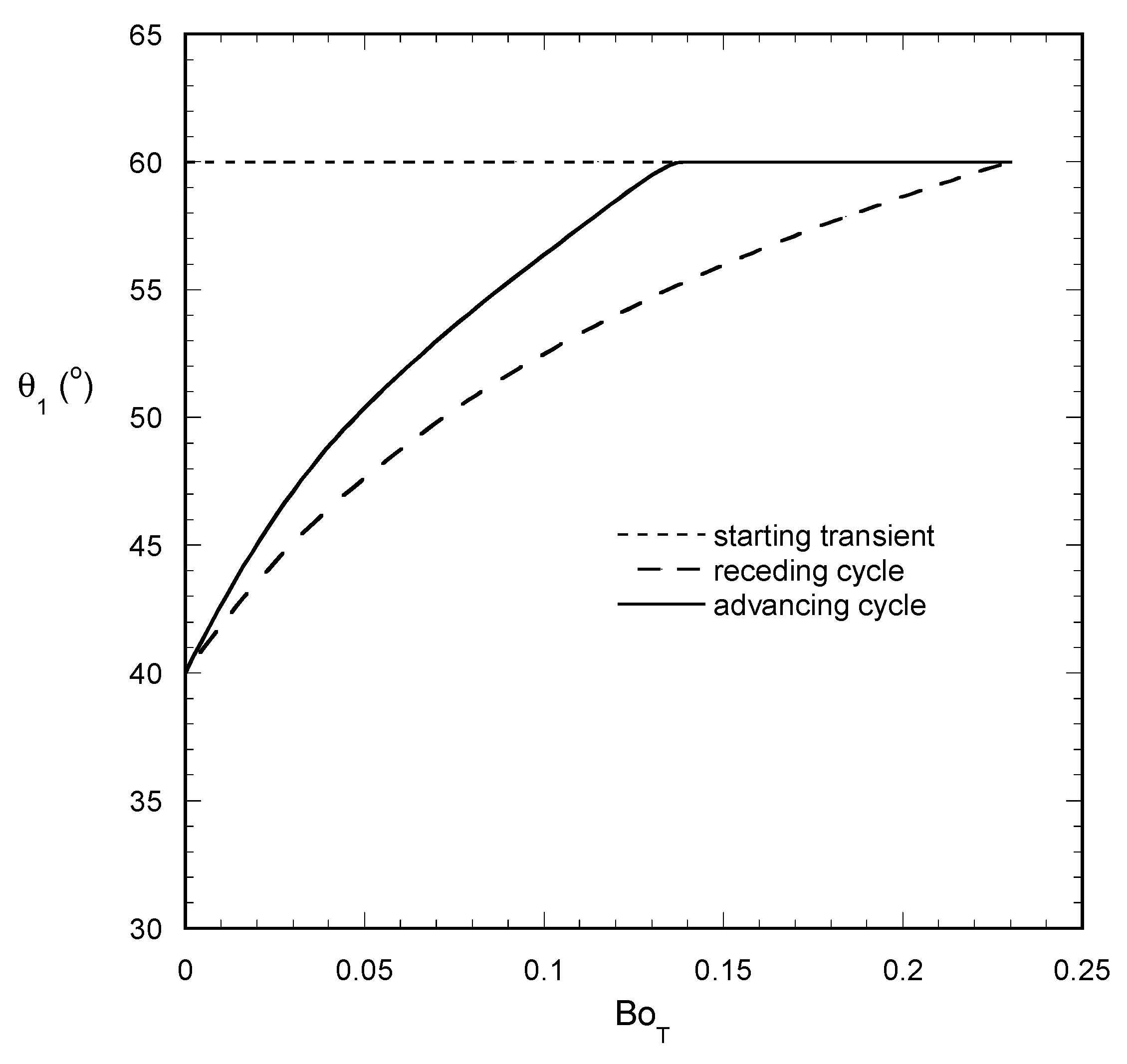
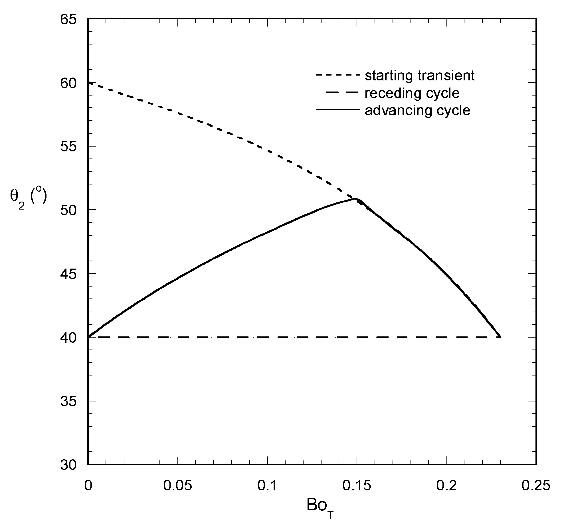
The oscillating force scenario is examined next. It is noted that the imparted oscillations are simultaneous for both components in order to keep their ratio constant (i.e., increasing and decreasing rotation speed for constant tilting angle in the absence of gravity). After the initial transient, the droplet gets into a steady periodic behavior. Interestingly enough, this behavior is quite different than the one found for constant Bo_N since not only the contact angles but also the droplet length varies periodically. The evolution of droplet length β, front angle θ₁ and rear angle θ₂ for periodic forces oscillation is shown in Figure 3, Figure 4 and Figure 5, respectively. The periodic cycle advancing part (i.e., increasing forces) contains a part in which the droplet length is constant and the angle θ₁ increases. As the point θ₁ reaches the value θ_a (advancing contact angle), the drop length starts increasing up to the critical point for sliding. Then, at the receding cycle, the length of the droplet decreases and the angle θ₁ goes from the advancing angle to the receding angle value. Even more interesting is the behavior of the angle θ₂ which at the receding cycle retains always the value θ_r. At the advancing cycle, it increases as far as length β remains constant acquiring a maximum at the point of β transition (from constant to increasing) and then decreases up to the critical point for sliding.

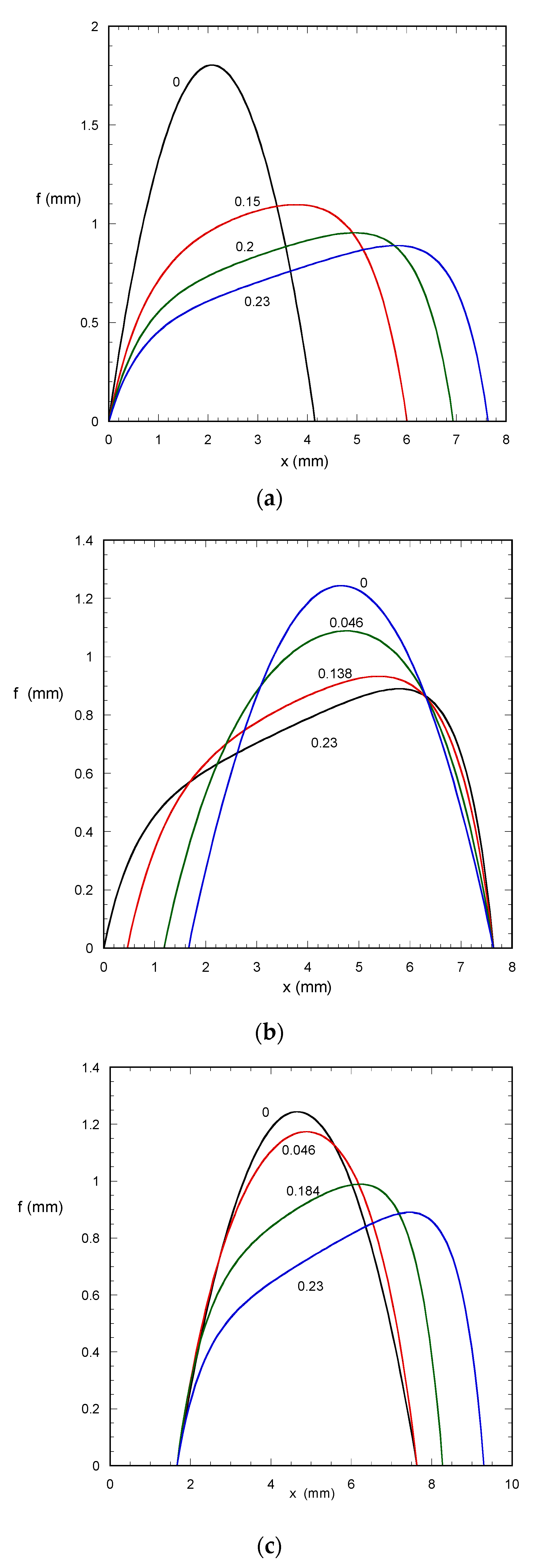
Typical droplet profiles that correspond to the results shown in Figure 3, Figure 4 and Figure 5 are presented in Figure 6 for periodic forcing and Bo_N = 12 Bo_T. It must be noted that for clarity in the presentation the scales at the two axes are different leading to distorted views of the droplet profiles. Figure 6a refers to the starting transient. As Bo_T increases, the symmetry is destroyed but also the length increases due to increase of Bo_N. The receding cycle profiles are shown in Figure 6b. The angle θ₂ has the value θ_r at the beginning of the cycle. The reduction of tangential force leads to increase of the angle θ₂, but the reduction of the normal force leads to its decrease which overall prevails leading to retraction of the rear contact line edge. Therefore, the rear contact line retraction is due to the reduction of the normal force. The front contact line does not retract due to the higher value of θ₁ than θ₂ in the beginning of the receding cycle. The cycle ends with a symmetric drop (zero tangential force) with angles at their receding values. 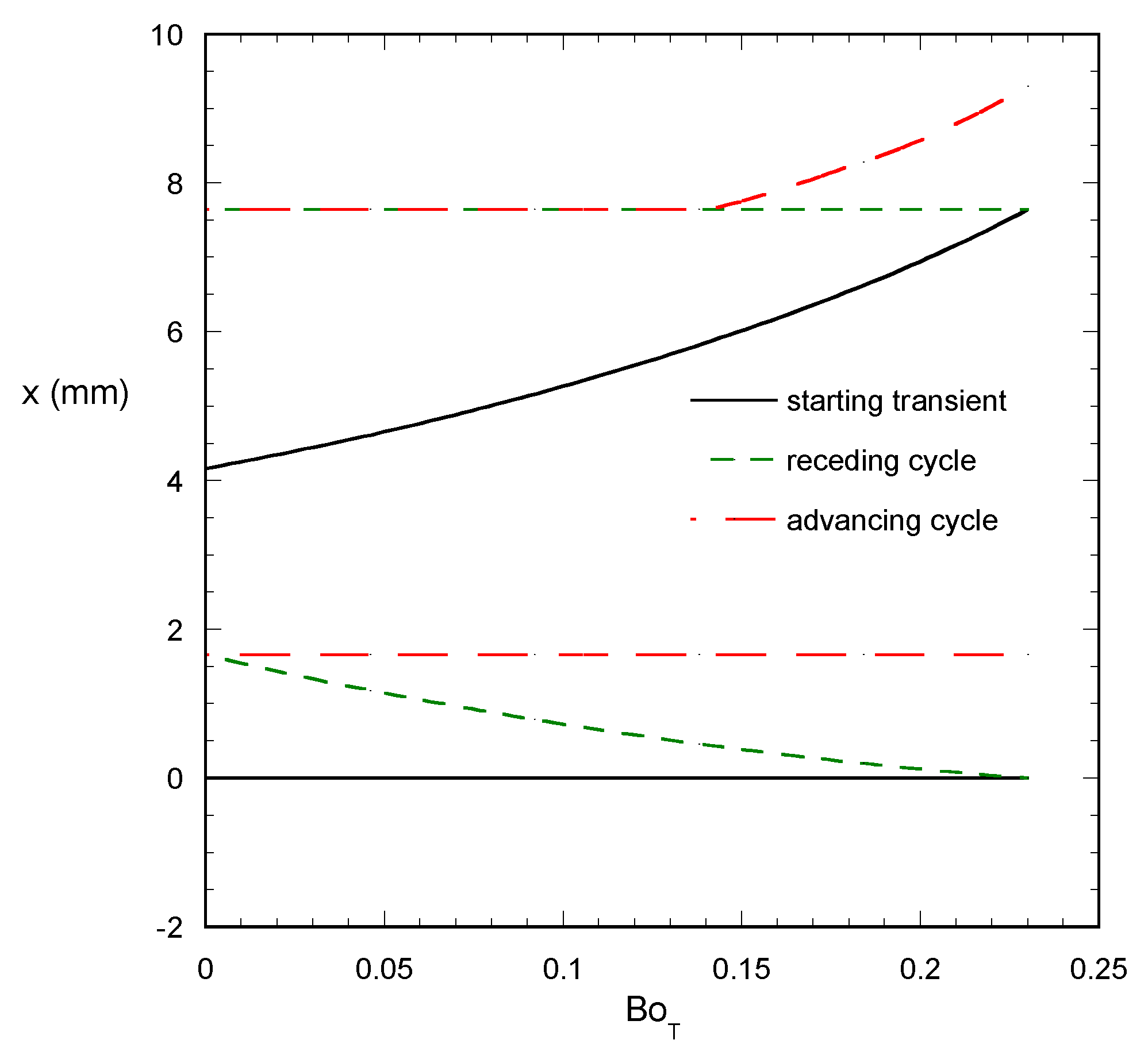The profiles for the advancing cycle are shown in Figure 6c. Initially, the droplet retains its length and both angles increase. At some point, the front angle reaches the advancing value, so the droplet length starts increasing and the rear angle starts decreasing. The front contact line edge moves leading, at the end of the cycle, to the same droplet shape as in the start of the cycle but at a different physical (spatial) position (see the x values of both edges). Such a behavior cannot be identified by the parameter variation appearing in Figure 3, Figure 4 and Figure 5. To better identify the situation, the variation of the physical position of the two contact line edges of the droplet during one cycle is presented in Figure 7. The region between the two lines in this figure (for each cycle) corresponds to the physical space occupied by the droplet. From this figure, it is clear how the droplet initially expands, then, when it gets in the oscillating regime, retracts and, finally, expands again but with a different fixed point. This motion pattern appears in each oscillation cycle leading to an effective overall droplet motion (shift by 1.66 mm per cycle) which is exclusively due to the simultaneous variation of Bo_N with Bo_T. The situation arising here has a very interesting sequence: The macroscopic motion of the drop cannot be identified as spreading (dominated by surface energy) or sliding (dominated by hydrodynamics) in case of complex force scenarios.

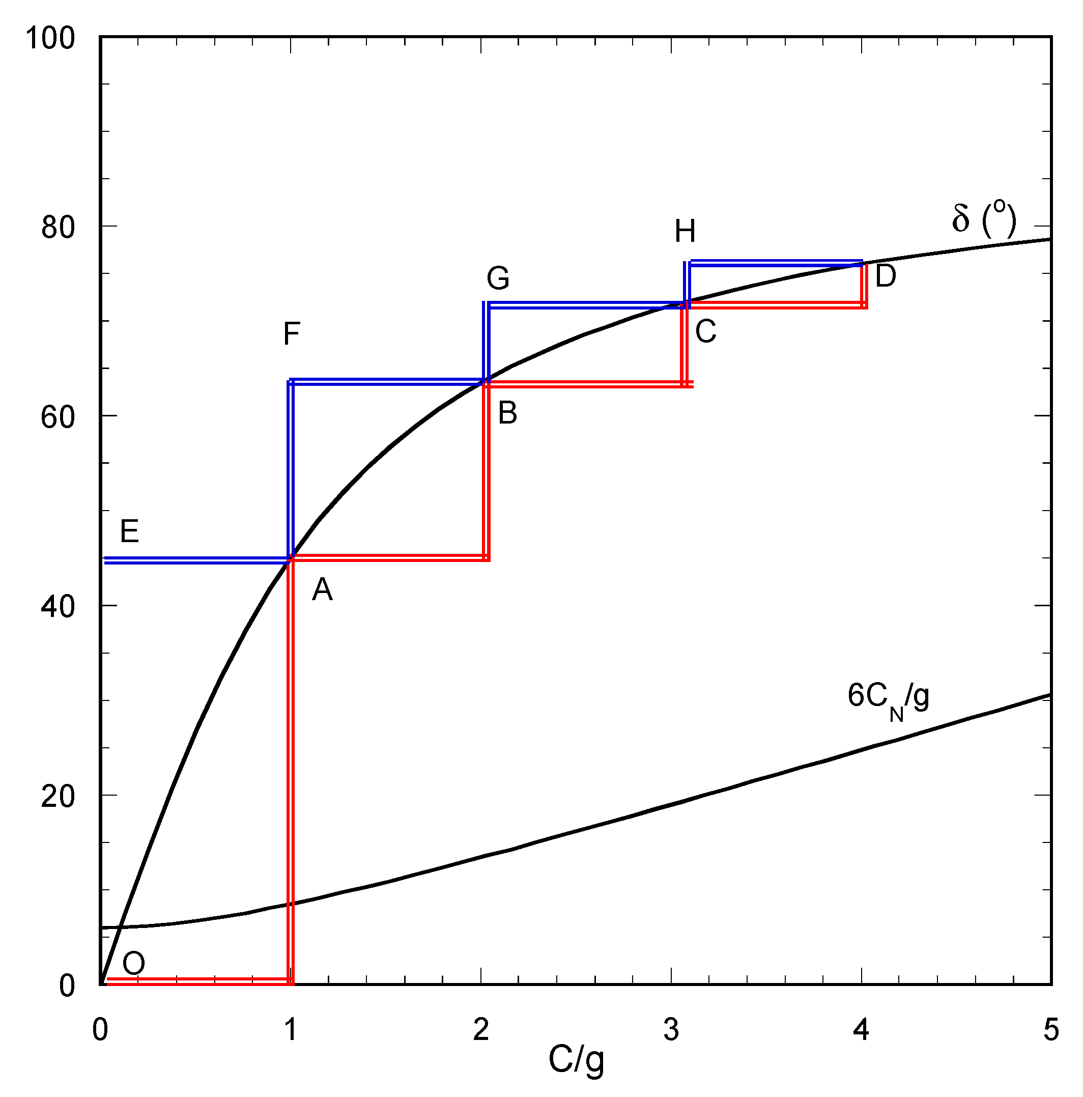
The scenarios of Bo_N–Bo_T variation examined up to now appear idealized in the absence of gravity but in practice terrestrial gravity is always present so their realization is rather cumbersome. Let us consider the very basic case of increasing the normal force while keeping zero the tangential force. To realize this in the absence of gravity the tilting angle should be 90° (vertical substrate parallel to axis of rotation). However, in the presence of gravity, the tilting angle must vary simultaneously with the rotation speed in order for the tangential component of gravity and rotation to be counterbalanced. This implies a tilting angle of 90° in which the tangential acting of gravity is present. Let C be the rotational acceleration magnitude and δ the inwards tilting angle. The condition of zero tangential force leads to C/g = tan (δ) which means that the rotation speed and the tilting angle must evolve simultaneously satisfying always this condition. The normal acceleration is given by C_N/g = cos (δ) + tan (δ) sin (δ).

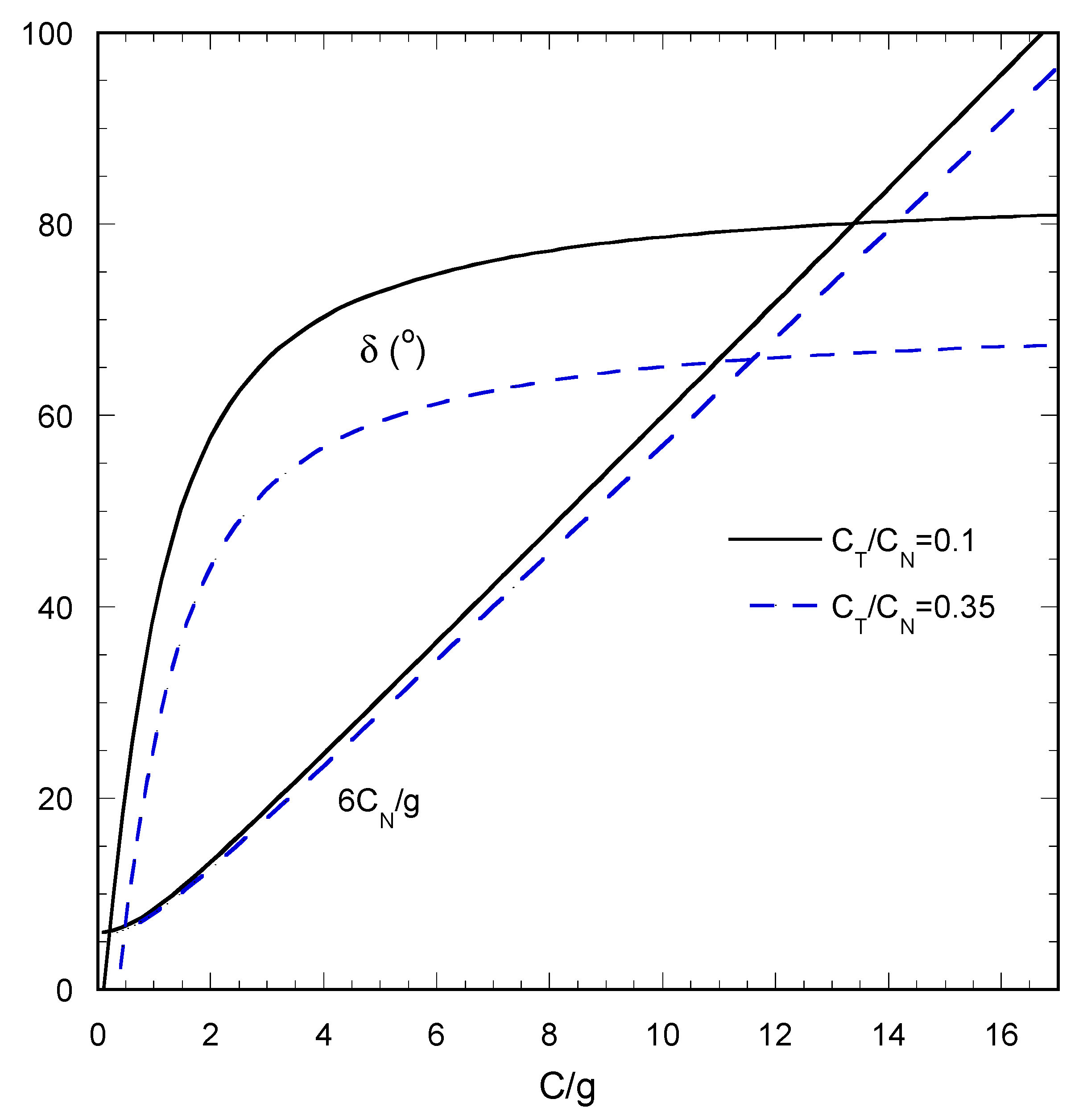
The scenario of constant ratio of acceleration components examined above is discussed next. In the absence of gravity this corresponds to a constant value of δ as already noticed. An analysis in the presence of gravity leads to

$$\mathsf{\delta }={\tan }^{-1}(\frac{\mathrm{C}/\mathrm{g}-{\mathrm{C}}_{\mathrm{T}}/{\mathrm{C}}_{\mathrm{N}}}{1+\mathrm{C}({\mathrm{C}}_{\mathrm{T}}/{\mathrm{C}}_{\mathrm{N}})/\mathrm{g}})$$

(21)

The required variation of δ with C for two values of the component ratio is shown in Figure 8. The general shape of the δ vs. C curve is similar to the case of zero C_T. The normal acceleration component is also shown in the figure. The form of the function δ vs. C indicates that the required trajectory is technically quite difficult to be exactly followed. There is large sensitivity with respect to rotational speed for small speeds and with respect to the tilting angle for large speeds. In practice, the trajectory can be followed only in discrete steps which, even if they are small, they still create excess forces. The influence of these forces can be assessed employing the analytical droplet model. In order to demonstrate the procedure a very coarse (four steps) stepwise approximation of the continuous δ–C curve for zero tangential force is considered. There are two routes to achieve this: (i) first vary the tilting angle δ and then vary C (i.e., rotational velocity) in each step (blue line at the left of continuous curve in Figure 9) and (ii) first vary C and then vary δ (red line at the right of continuous curve in Figure 9). Computations show that the second route leads to larger tangential forces so droplet profiles are shown only for the first route. The same droplet parameters as before are considered except for θ_r which is assumed to be zero to avoid droplet sliding. 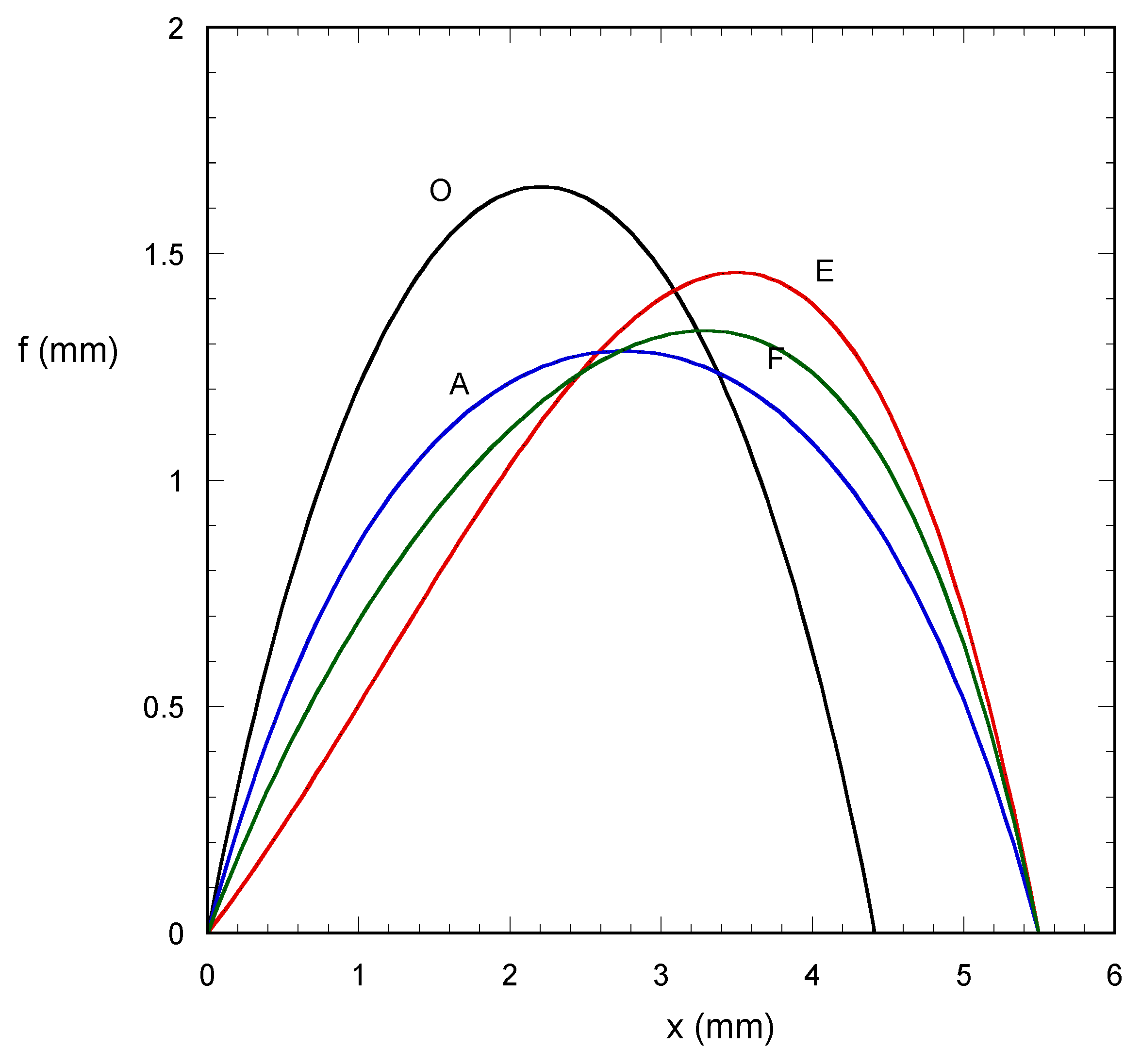It is also assumed that Bo_N = C_N/2.5. Some profiles for specified positions along the blue route are shown in Figure 10.

At position E, the variation of δ without the counterbalancing effect of C leads to a significant tangential force which for θ_r = 40° would lead to droplet sliding. The tangential force increases the contact line length of the droplet. At the other displayed positions (A, F), the droplet length remains constant whereas the shape alternates between symmetric (A position at the continuous curve in Figure 9) and asymmetric (F position outside the continuous curve in Figure 9) with a decreasing difference between the two states as C increases.

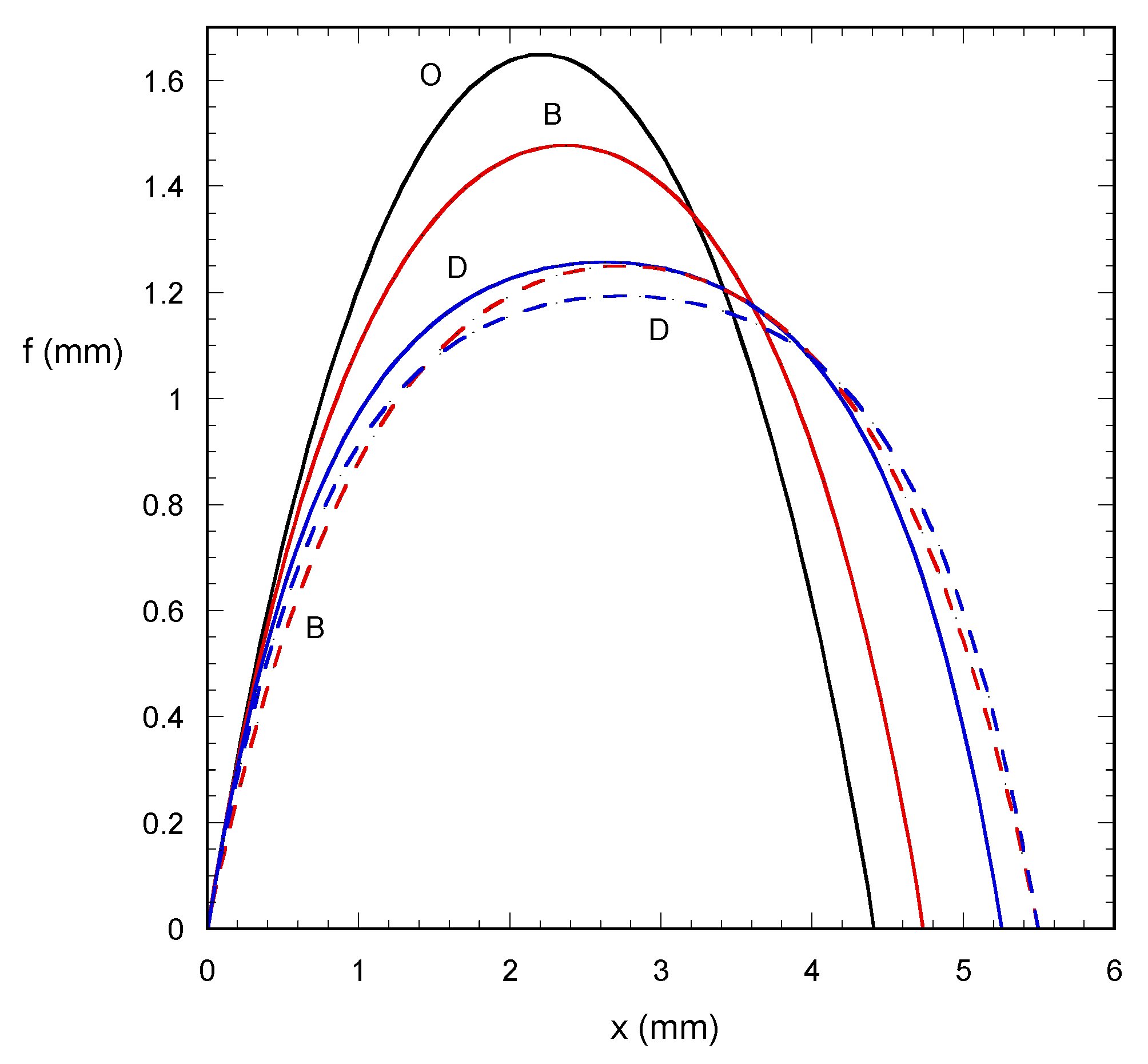
The comparison of droplet profiles at positions B and D reached through the continuous curve and through the left stepwise one (blue line in Figure 9) is presented in Figure 11. The difference between the two routes in position B (red curves) is very large since the droplet has been elongated abruptly by the tangential force raised by the stepwise route. As the normal force increases the droplet, the following continuous route is progressively elongated leading to small differences between the profiles from the two trajectories at position D. The above case study reveals the complexity of the problem combining the technical limitations on applied forces variation and the physicochemical aspect of droplet spreading. This is why the simple model presented herein is useful to assess different experimental procedures and as a starting point for more detailed calculations. A partially qualitative confirmation of the resulting behavior regarding the oscillations of tangential force and the force step scenarios can be found in [8].

The main aspect of the model that creates the droplet evolution is the interaction between the applied forces scenario and the onset of motion condition (θ ≤ θ_a and θ ≥ θ_r). In this respect, the conclusions are expected to be qualitatively valid for real droplets. However, in pursuing a quantitative analysis it has been implied, [8], that the main deviation of the present approximation from reality is due to the linearization of the Young–Laplace equation and not due to the reduced dimensionality. It is reminded that the linearization is valid in the limit of very omniphilic surfaces. The present model serves the scope of being the simplest case (and the only analytic one) capable of reproducing the qualitative droplet behavior under complex force scenarios. Our final aim is to relax the simplifications using approximate solutions of the governing equations.

4. Conclusions

It is shown that the two-dimensional linearized Young–Laplace equation for a sessile droplet on a omniphilic surface under a uniform body force of arbitrary direction can be solved analytically to give an explicit shape profile function. The particular simplification has been used extensively in the past to model sliding behavior [22]. In case of nontrivial scenarios of the force magnitude and direction evolution under quasisteady conditions (evolution characteristic time much smaller than droplet hydrodynamic characteristic time), the complete droplet dynamics is described by two algebraic equations combined to the requirement that the two contact angles must always have values between the receding and the advancing one. Several scenarios of force evolution are examined (mainly based on the rotating-tilting configuration) and it is found that very interesting drop behavior emerge even by using a so primitive model. It is expected that the model can qualitative describe the actual droplet behavior but further research is needed to account for its quantitative performance with respect to more complicated models.