Polynomial Chaos Expanded Gaussian Process

Abstract

In complex and unknown processes, global models are fitted over the entire input domain but often tend to perform poorly whenever the response surface exhibits non-stationary behavior and varying smoothness. A common approach is to use local models, which requires partitioning the input domain into subdomains and training multiple models, thereby adding significant complexity. Recognizing this limitation, this study addresses the need for models that represent the input–output relationship consistently over the full domain while still adapting to local variations in the response. It introduces a novel machine learning approach: the Polynomial Chaos Expanded Gaussian Process (PCEGP), leveraging polynomial chaos expansion to calculate input-dependent hyperparameters of the Gaussian process (GP). This provides a mathematically interpretable approach that incorporates non-stationary covariance functions and heteroscedastic noise estimation to generate locally adapted models. The model performance is compared to different algorithms in benchmark tests for regression tasks. The results demonstrate low prediction errors of the PCEGP, highlighting model performance that is often competitive with or better than previous methods. A key advantage of the presented model is its interpretable hyperparameters along with training and prediction runtimes comparable to those of a standard GP.

1. Introduction

System modeling of real processes occurs within a specific global experimental space. A widely used choice for modeling unknown system behavior is the Gaussian process (GP), introduced in [1]. The GP is often used with stationary covariance functions for regression tasks. This assumes that the smoothness of the response is constant over the experimental space. As demonstrated in [2], predicting a function with a varying smoothness using stationary covariance functions leads to increased prediction errors in areas with abrupt variations. To reduce the prediction errors, more experiments could be performed in those areas with abrupt variations, which lead to heterogeneous and non-uniform data point densities. According to [2], stationarity assumes an almost uniform input design. When non-stationary covariance functions are used, advantages have been demonstrated for data whose response surface exhibits input-dependent smoothness, e.g., in [2,3].

Therefore, models are needed that can handle non-uniform densities of training data and varying smoothness of the target function across the input domain. In addition, such models should be able to handle heteroscedastic noise, as presented, e.g., in [4,5].

One approach to account for heterogeneous data density across the input space in GPs is to use non-stationary covariance functions. Non-stationarity allows the input–output relationship to vary with the input location, enabling the GP to adapt its smoothness and variance locally in the input space [6].

In [7], a non-stationary version of the Matérn covariance function is presented, which allows non-stationary behavior to be modeled in data. A second-level GP is used in [6] to calculate the lengthscale parameters of the first-level GP in order to model non-stationary behavior. For the anisotropic case, this leads to a second-level GP for each input, which can be computationally expensive with an increasing number of inputs.

In [8], the use of deep Gaussian processes (DGPs), first introduced in [9], with Bayesian optimization (BO) is investigated. The non-stationarity of data is modeled by considering a functional composition of stationary GPs, providing a multiple-layer structure. The DGP approach has also shown promising results in learning surrogate models with as little data as possible, as presented in [10]. However, the DGP approach leads to a more difficult interpretability and is challenging for model training due to the nested structure.

Furthermore, there are approaches that use local experts to model non-stationary behavior, as presented in [11]. In [3], input partitioning with hierarchical hyperplane kernels (HHKs) for GPs is used to achieve non-stationarity. Such approaches require training of several different models.

In [12], the non-stationarity of GPs is achieved by using a deep neural network (DNN) for hyperparameter estimation of the GP depending on the input data. Typical DNNs are a type of black box learning, the training process of a DNN lacks transparency. While their training procedure is well understood, the internal representations and decision-making process of a trained network are difficult to interpret [13].

These approaches result in either a structural limitation of the model, a computationally expensive model, the need for different local models, or a model that is difficult to interpret. In this work, a mathematically interpretable method for parameterization of non-stationary covariance functions and heteroscedastic noise estimation is presented.

Here, the novel combination of polynomial chaos expansions (PCEs) and GPs, called the Polynomial Chaos Expanded Gaussian Process (PCEGP), is presented. The PCE is utilized to calculate input-dependent hyperparameters of the GP. This approach provides the ability to model the global and local behavior of a complex process with only one model and low computational cost since evaluating a polynomial function requires only basic arithmetic operations. As shown in [14], PCE-based models work well for machine learning (ML) regression on small datasets. In addition, the PCE representation allows the computation of statistical moments and sensitivities of the output with respect to the inputs [15,16].

This paper is structured as follows. First, a short introduction and further references to the PCE and GPs are given in Section 2. In Section 3, the ML approach with the novel combination of the PCE and GP is introduced. Then, the method to generate non-stationary covariance functions and the heteroscedastic noise estimation are introduced. After that, the hyperparameter optimization (HPO) strategy for the PCEGP is presented. The evaluation of the new ML approach using various benchmark datasets is described in Section 5. The results illustrate ability of the proposed approach to achieve low prediction errors across diverse applications, underscoring a model performance that competes with or surpasses previous methods. Finally, a summary and outlook for future work are given in Section 6.

2. Background and Related Work

In this section, the necessary components for the novel ML approach are presented. This includes the PCE and GP.

2.1. Polynomial Chaos Expansion

The PCE, presented in [17], is a popular method in uncertainty quantification (UQ) of models which are parameterized by independent random variables with extensions to dependent variables [18]. The term “chaos” in PCE originates from Wiener’s homogeneous chaos theory and denotes the representation of random quantities by orthogonal polynomial expansions in UQ [17,19]. By viewing the model as an input–output map, the effect of input to output uncertainties can be assessed in UQ [20]. The PCE allows the modeling of different data distributions with different kinds of polynomial bases.

In the case of UQ for high-fidelity models, a large number of simulations is required. To avoid the computational load, surrogate models can be used. One of the most widely used methods to build a surrogate model in UQ is generalized polynomial chaos. The PCE is well suited for the approximation of functions with random variables because of the orthogonality of the polynomial basis to the probability measure of the variables [21].

In general, the polynomial chaos expansion (PCE) is defined by

$$f\left(\mathit{\xi }\right)\approx \sum _{{\mathit{k}}_{\alpha }\in {\mathcal{K}}_{\alpha }}{\alpha }_{{\mathit{k}}_{\alpha }}{\mathrm{\Phi }}_{{\mathit{k}}_{\alpha }}\left(\mathit{\xi }\right),$$

(1)

where $f\left(\mathit{\xi }\right)\in \mathbb{R}$ denotes the approximated function by the PCE, depending on the random variables $\mathit{\xi }=({\xi }_1,{\xi }_2,\dots ,{\xi }_{n_{\xi }})$. The coefficients of the expansion are ${\alpha }_{{\mathit{k}}_{\alpha }}$, and the polynomial basis functions are ${\mathrm{\Phi }}_{{\mathit{k}}_{\alpha }}\left(\mathit{\xi }\right)$. The multi-index ${\mathit{k}}_{\alpha }=(k_{\alpha ,1},k_{\alpha ,2},\dots ,k_{\alpha ,n_{\mathit{\xi }}})$ is a vector of indices, where $n_{\mathit{\xi }}$ denotes the number of random input variables, and ${\mathcal{K}}_{\alpha }$ is a set of multi-indices.

The multivariate polynomial basis functions ${\mathrm{\Phi }}_{{\mathit{k}}_{\alpha }}\left(\mathit{\xi }\right)$ are constructed as products of univariate polynomials ${\varphi }_{k_{\alpha ,i}}\left({\xi }_i\right)$, which are orthogonal with respect to the marginal distribution of ${\xi }_i\in \mathbb{R}$, and are defined as

$${\mathrm{\Phi }}_{{\mathit{k}}_{\alpha }}\left(\mathit{\xi }\right)=\prod _{i=1}^{n_{\xi }}{\varphi }_{k_{\alpha ,i}}\left({\xi }_i\right).$$

(2)

The orthogonality property of the polynomial basis functions ${\mathrm{\Phi }}_{{\mathit{k}}_{\alpha }}\left(\mathit{\xi }\right)$ with respect to the probability density function $p\left(\mathit{\xi }\right)$ of the random variables $\mathit{\xi }$ can be expressed as

$${\int }_{\mathrm{\Omega }}{\mathrm{\Phi }}_{{\mathit{k}}_{\alpha }}\left(\mathit{\xi }\right){\mathrm{\Phi }}_{{\mathit{j}}_{\alpha }}\left(\mathit{\xi }\right)p\left(\mathit{\xi }\right)\mathrm{d}\mathit{\xi }=\left\{\begin{array}{cc}{\gamma }_{{\mathit{k}}_{\alpha }},\hfill & \mathrm{if}{\mathit{k}}_{\alpha }={\mathit{j}}_{\alpha }\hfill \\ 0,\hfill & \mathrm{if}{\mathit{k}}_{\alpha }\ne {\mathit{j}}_{\alpha },\hfill \end{array}\right.$$

(3)

where $p\left(\mathit{\xi }\right)$ is the joint probability density function of the random variables, ${\gamma }_{{\mathit{k}}_{\alpha }}$ is a normalization constant associated with the multi-index ${\mathit{k}}_{\alpha }$, and $\mathrm{\Omega }$ denotes the domain over which the random variables $\mathit{\xi }$ are defined. This domain $\mathrm{\Omega }$ encompasses all possible values of $\mathit{\xi }$ for which the probability density function $p\left(\mathit{\xi }\right)$ is non-zero. This condition can also be compactly represented using the Kronecker delta ${\delta }_{{\mathit{k}}_{\alpha }{\mathit{j}}_{\alpha }}$

$${\int }_{\mathrm{\Omega }}{\mathrm{\Phi }}_{{\mathit{k}}_{\alpha }}\left(\mathit{\xi }\right){\mathrm{\Phi }}_{{\mathit{j}}_{\alpha }}\left(\mathit{\xi }\right)p\left(\mathit{\xi }\right)\mathrm{d}\mathit{\xi }={\gamma }_{{\mathit{k}}_{\alpha }}{\delta }_{{\mathit{k}}_{\alpha }{\mathit{j}}_{\alpha }},$$

(4)

where ${\delta }_{{\mathit{k}}_{\alpha }{\mathit{j}}_{\alpha }}=1$ if ${\mathit{k}}_{\alpha }={\mathit{j}}_{\alpha }$ and 0 otherwise.

The orthogonality of the basis functions ensures that the PCE provides a stable and efficient representation of the target function $f\left(\mathit{\xi }\right)$. This orthogonality simplifies the computation of the expansion coefficients ${\alpha }_{{\mathit{k}}_{\alpha }}$ by ensuring that each coefficient can be determined independently of the others, reducing the complexity of the optimization process.

The summation in the general definition runs over all possible multi-indices ${\mathit{k}}_{\alpha }\in {\mathcal{K}}_{\alpha }$, the expansion is generally infinite. To limit the expansion to a finite number of terms, the infinite summation is truncated to a finite sum with a maximum polynomial degree $q\in {\mathbb{N}}_0$

$$f\left(\mathit{\xi }\right)\approx \sum _{{\mathit{k}}_{\alpha }\in {\mathcal{K}}_{\alpha ,q}}{\alpha }_{{\mathit{k}}_{\alpha }}{\mathrm{\Phi }}_{{\mathit{k}}_{\alpha }}\left(\mathit{\xi }\right),$$

(5)

where ${\mathcal{K}}_{\alpha ,q}=\left\{{\mathit{k}}_{\alpha }\in {\mathcal{K}}_{\alpha }|{\sum }_{i=1}^{n_{\mathit{\xi }}}{k}_{\alpha ,i}\le q\right\}$ is the set of multi-indices whose total degree ${\sum }_{i=1}^{n_{\mathit{\xi }}}{k}_{\alpha ,i}$ is less than or equal to the maximum degree q.

The choice of the polynomial basis function for each random variable ${\xi }_i$ depends on the distribution of ${\xi }_i$. There exist several orthogonal polynomial bases and their corresponding probability density functions. For example, for a uniformly distributed random variable ${\xi }_i\sim \mathcal{U}(-1,1)$, the corresponding univariate orthogonal polynomials ${\varphi }_{k_{\alpha ,i}}\left({\xi }_i\right)$ are given by the Legendre polynomials ${\mathrm{Le}}_{k_{\alpha ,i}}\left({\xi }_i\right)$, which on the interval ${\xi }_i\in [-1,1]$ can be defined as

$${\varphi }_{k_{\alpha }}\left({\xi }_i\right)={\mathrm{Le}}_{k_{\alpha ,i}}\left({\xi }_i\right)={\displaystyle \frac{1}{2^{k_{\alpha ,i}}{k}_{\alpha ,i}!}}{\displaystyle \frac{{\mathrm{d}}^{k_{\alpha ,i}}}{\mathrm{d}{\xi }_i^{k_{\alpha }}}}{\left({\xi }_i^2-1\right)}^{k_{\alpha }}.$$

(6)

with the associated probability density function

$$p\left({\xi }_i\right)={\displaystyle \frac{1}{2}},{\xi }_i\in [-1,1],$$

(7)

and $p\left({\xi }_i\right)=0$ otherwise.

The number of coefficients $N_{\alpha }$ depends on the maximum polynomial degree q and the number of random input variables $n_{\xi }$. It can be calculated by

$$N_{\alpha }=\left({\displaystyle \genfrac{}{}{0pt}{}{n_{\xi }+q}{q}}\right)={\displaystyle \frac{(n_{\xi }+q)!}{n_{\xi }!q!}}.$$

(8)

The number of coefficients $N_{\alpha }$ grows rapidly with increasing polynomial degree q and the number of random input variables $n_{\xi }$. Therefore, it is crucial to keep the polynomial degree moderate or to reduce the number of random input variables using techniques such as principal component analysis (PCA) [22], to manage the rapid increase in the number of coefficients and mitigate the computational complexity of the expansion.

Another method to reduce the number of coefficients and the computational complexity is the application of sparse polynomial chaos expansion (SPCE), as presented in [23]. One way to achieve sparsity in the PCE is to apply elastic net (EN) regularization [24], which combines both L1 (Lasso) and L2 (Ridge) penalties. Let $\mathit{\alpha }\equiv {\left\{{\alpha }_{{\mathit{k}}_{\alpha }}\right\}}_{{\mathit{k}}_{\alpha }\in {\mathcal{K}}_{\alpha }}\in {\mathbb{R}}^{N_{\alpha }}$ denote the vector of PCE coefficients. The elastic net optimization problem is then defined as

$$\begin{array}{cc}\hfill {\mathit{\alpha }}^{*}=arg\underset{\mathit{\alpha }\in {\mathbb{R}}^{N_{\alpha }}}{min}& \left[\mathcal{L}\left(\alpha \right)+\lambda \left(\beta \sum _{{\mathit{k}}_{\alpha }\in {\mathcal{K}}_{\alpha }}\left|{\alpha }_{{\mathit{k}}_{\alpha }}\right|\right)+\lambda \left((1-\beta )\sum _{{\mathit{k}}_{\alpha }\in {\mathcal{K}}_{\alpha }}{\alpha }_{{\mathit{k}}_{\alpha }}^2\right)\right],\hfill \\ \hfill & \underset{\mathrm{L}1\left(\mathrm{Lasso}\right)\mathrm{penalty}}{\underbrace{\phantom{xxxxxxxx}}}\underset{\mathrm{L}2\left(\mathrm{Ridge}\right)\mathrm{penalty}}{\underbrace{\phantom{xxxxxxx}}}\hfill \end{array}$$

(9)

where $\mathcal{L}\left(\mathit{\alpha }\right)$ denotes the loss function (e.g., mean squared error), $\lambda \in {\mathbb{R}}^{+}$ is the regularization parameter that controls the overall strength of regularization, and $\beta \in [0,1]$ is a parameter that determines the balance between the L1 and L2 penalties. This approach encourages sparsity while maintaining some of the stability properties of ridge regression and helps to prevent overfitting, especially in cases where the polynomial degree is chosen too high.

The application of the PCE beyond its typical use case for UQ has been demonstrated in [14,25]. In [14], it is shown how the PCE can be used for ML regression. In [25], a combination of the PCE and GP for ML is presented, in which the PCE is used to describe the global behavior of the computational model while the GP describes the local variability of the model. This combination of the PCE and GP is completely different to the approach developed in this work.

2.2. Gaussian Process

The GP is a probabilistic ML approach using covariance structures [1]. The principle advantage over other covariance-based approaches is given by an uncertainty measurement of the predictions.

A GP is a collection of random variables. Each finite number of these random variables has a joint Gaussian distribution. In the following the GP is considered for regression, where the training data are denoted as $\mathcal{D}={\{{\mathit{x}}_i,y_i\}}_{i=1}^N$ with ${\mathit{x}}_i\in {\mathbb{R}}^{n_x}$ and $y_i\in \mathbb{R}$. The number of training points is denoted with N and the number of inputs is denoted with $n_x$.

The mean function $m\left(\mathit{x}\right)$ and the covariance function $k(\mathit{x},{\mathit{x}}^{\prime })$, also called kernel function, completely describe the GP

$$f\left(\mathit{x}\right)\sim \mathcal{GP}\left(m\left(\mathit{x}\right),k(\mathit{x},{\mathit{x}}^{\prime })\right),$$

(10)

where $\mathit{x}$ and ${\mathit{x}}^{\prime }$ represent input data points. In contrast to the random input variables $\mathit{\xi }$ used in the PCE construction, $\mathit{x}$ denotes fixed input locations at which the GP is evaluated (i.e., realizations of $\mathit{\xi }$). Most ML applications have a large number of input parameters, e.g., in chemical engineering [26], autonomous driving [27], and energy consumption forecasting [28]. This results in a high-dimensional feature space for the learning algorithm. For distance-based ML algorithms, this leads to the so-called curse of dimensionality [29]. To avoid this, unimportant features can be removed with automatic relevance determination (ARD) [30] or by techniques presented in [31]. For GPs, the ARD is realized by introducing a lengthscale parameter for each feature [32].

A common choice for the stationary covariance function of the GP is the squared exponential kernel; see [1]. It is defined by

$$k\left(\mathit{x},{\mathit{x}}^{\prime }\right)={\sigma }_{\mathrm{f}}^{2}exp\left(-{\displaystyle \frac{\parallel \mathit{x}-{\mathit{x}}^{\prime }{\parallel }^2}{2l^2}}\right),$$

(11)

with the correlation lengthscale $l\in {\mathbb{R}}^{+}$ and the signal variance ${\sigma }_{\mathrm{f}}^2\in {\mathbb{R}}^{+}$. There exist also extensions of this covariance function, e.g., the squared exponential covariance function with ARD, which is defined by

$$k\left(\mathit{x},{\mathit{x}}^{\prime }\right)={\sigma }_{\mathrm{f}}^{2}exp\left(-{\displaystyle \frac{1}{2}}{\left(\mathit{x}-{\mathit{x}}^{\prime }\right)}^{⊺}\mathit{L}\left(\mathit{x}-{\mathit{x}}^{\prime }\right)\right),$$

(12)

with the lengthscale matrix $\mathit{L}=\mathrm{diag}{\left(\left[l_1\dots l_{n_x}\right]\right)}^{-2}$. The lengthscale matrix includes one lengthscale parameter $l_i\in {\mathbb{R}}^{+}$ for each input. A further extension is presented in [4], where the authors used a non-stationary generalization of the squared exponential covariance function, defined as

$$k\left(\mathit{x},{\mathit{x}}^{\prime }\right)={\sigma }_{\mathrm{f}}\left(\mathit{x}\right){\sigma }_{\mathrm{f}}\left({\mathit{x}}^{\prime }\right)\sqrt{{\displaystyle \frac{2l\left(\mathit{x}\right)l\left({\mathit{x}}^{\prime }\right)}{l^2\left(\mathit{x}\right)+l^2\left({\mathit{x}}^{\prime }\right)}}}\exp \left(-{\displaystyle \frac{\parallel \mathit{x}-{\mathit{x}}^{\prime }{\parallel }^2}{l^2\left(\mathit{x}\right)+l^2\left({\mathit{x}}^{\prime }\right)}}\right).$$

(13)

In this extension, the hyperparameters ${\sigma }_{\mathrm{f}}\left(\mathit{x}\right)\in {\mathbb{R}}^{+}$ and $l\left(\mathit{x}\right)\in {\mathbb{R}}^{+}$ are data point-dependent to model non-stationarity.

The hyperparameters are used to fit the model to the given data. In the following, all hyperparameters of the GP are summarized in $\mathit{\theta }\in {\mathbb{R}}^{n_x+2}$, which leads to the covariance matrix

$$\mathit{K}\left(\mathit{X},\mathit{X},\mathit{\theta }\right)=\mathit{K}\left(\mathit{X},\mathit{X},\mathit{L},{\sigma }_{\mathrm{f}}\right)+{\sigma }_{\mathrm{n}}^2\mathit{I}.$$

(14)

The noise variance ${\sigma }_{\mathrm{n}}^2\in {\mathbb{R}}^{+}$ is used to model the noise in the data and also serves as hyperparameter of the GP.

In the following, $\mathit{K}\left(\mathit{X},\mathit{X}\right)\in {\mathbb{R}}^{N\times N}$ denotes the covariance matrix depending on the training data, and $\mathit{K}\left(\mathit{X},{\mathit{x}}^{*}\right)\in {\mathbb{R}}^N$ denotes the covariance vector depending on the training data and the next point ${\mathit{x}}^{*}$ to predict. The input training points of the whole dataset $\mathcal{D}$ are denoted as $\mathit{X}\in {\mathbb{R}}^{N\times n_x}$. The elements of the covariance matrix $\mathit{K}\left(\mathit{X},\mathit{X}\right)$ are calculated by the covariance function $k\left(\mathit{x},{\mathit{x}}^{\prime }\right)$ and are thus dependent on the training data $\mathcal{D}$ and the hyperparameters $\mathit{L}$, ${\sigma }_{\mathrm{f}}$, and ${\sigma }_{\mathrm{n}}$.

Usually, these hyperparameters are optimized by maximizing the log marginal likelihood (LML), which is given by

$$\begin{array}{c}\hfill \log p\left(\mathit{y}|\mathit{X}\right)=-{\displaystyle \frac{1}{2}}{\mathit{y}}^{⊺}\mathit{K}{\left(\mathit{X},\mathit{X}\right)}^{-1}\mathit{y}-{\displaystyle \frac{1}{2}}\log \left|\mathit{K}\left(\mathit{X},\mathit{X}\right)\right|-{\displaystyle \frac{N}{2}}\log \left(2\pi \right)\end{array}$$

under the assumption that $\mathit{y}\sim \mathcal{N}\left(0,\mathit{K}\left(\mathit{X},\mathit{X}\right)+{\sigma }_{\mathrm{n}}^2\mathit{I}\right)$ for the GP output. For the optimization of the hyperparameters with a gradient descent algorithm, the gradient of the LML is used and given by

$$\begin{array}{c}\hfill {\displaystyle \frac{\partial }{\partial {\mathit{\theta }}_i}}\log p\left(\mathit{y}|\mathit{X},\mathit{\theta }\right)={\displaystyle \frac{1}{2}}{\mathit{y}}^{⊺}\mathit{K}{\left(\mathit{X},\mathit{X}\right)}^{-1}{\displaystyle \frac{\partial }{\partial {\mathit{\theta }}_i}}\mathit{K}{\left(\mathit{X},\mathit{X}\right)}^{-1}\mathit{y}-{\displaystyle \frac{1}{2}}\mathrm{tr}\left(\mathit{K}{\left(\mathit{X},\mathit{X}\right)}^{-1}{\displaystyle \frac{\partial \mathit{K}\left(\mathit{X},\mathit{X}\right)}{\partial {\mathit{\theta }}_i}}\right).\end{array}$$

(15)

To predict an output based on a new input ${\mathit{x}}^{*}\in {\mathbb{R}}^{n_x}$ and the given dataset $\mathcal{D}$, the posterior distribution is defined by

$$\begin{array}{cc}\hfill \mu \left({\mathit{x}}^{*}\right)=& m\left({\mathit{x}}^{*}\right)+\mathit{K}{\left(\mathit{X},{\mathit{x}}^{*}\right)}^{⊺}\mathit{K}{\left(\mathit{X},\mathit{X}\right)}^{-1}\left(\mathit{y}-\mathit{m}\left(\mathit{X}\right)\right),\hfill \end{array}$$

(16)

$$\begin{array}{cc}\hfill {\sigma }^2\left({\mathit{x}}^{*}\right)=& k\left({\mathit{x}}^{*},{\mathit{x}}^{*}\right)-\mathit{K}{\left(\mathit{X},{\mathit{x}}^{*}\right)}^{⊺}\mathit{K}{\left(\mathit{X},\mathit{X}\right)}^{-1}\mathit{K}\left(\mathit{X},{\mathit{x}}^{*}\right),\hfill \end{array}$$

(17)

where $\mu \left({\mathit{x}}^{*}\right)\in \mathbb{R}$ denotes the mean prediction, ${\sigma }^2\left({\mathit{x}}^{*}\right)\in {\mathbb{R}}^{+}$ is the uncertainty prediction of the point to evaluate ${\mathit{x}}^{*}$, and $\mathit{m}\left(\mathit{X}\right)={\left[m\left({\mathit{x}}_1\right),\dots ,m\left({\mathit{x}}_N\right)\right]}^{⊺}$ denotes the vector of mean function evaluations $m\left(\mathit{x}\right)$ at the training inputs.

3. Polynomial Chaos Expanded Gaussian Processes

In this section, the novel ML approach as a combination of the PCE and GP is presented, where the PCE is used to calculate the hyperparameters of the GP. First, the general architecture and methodology of this approach is presented. After that, the hyperparameter optimization is described. Then, a runtime comparison is presented.

3.1. Architecture and Methodology

In the generic PCE formulation above, random variables are denoted by $\mathit{\xi }$, following the standard notation commonly used in uncertainty quantification. In the proposed PCEGP model, however, the GP inputs are denoted by $\mathit{x}$ and are treated as deterministic input data. Accordingly, the PCE is not used here as a standalone random-variable model but is evaluated at the scaled inputs ${\mathit{x}}_{\mathrm{s}}^{*}$ to parameterize input-dependent GP hyperparameters.

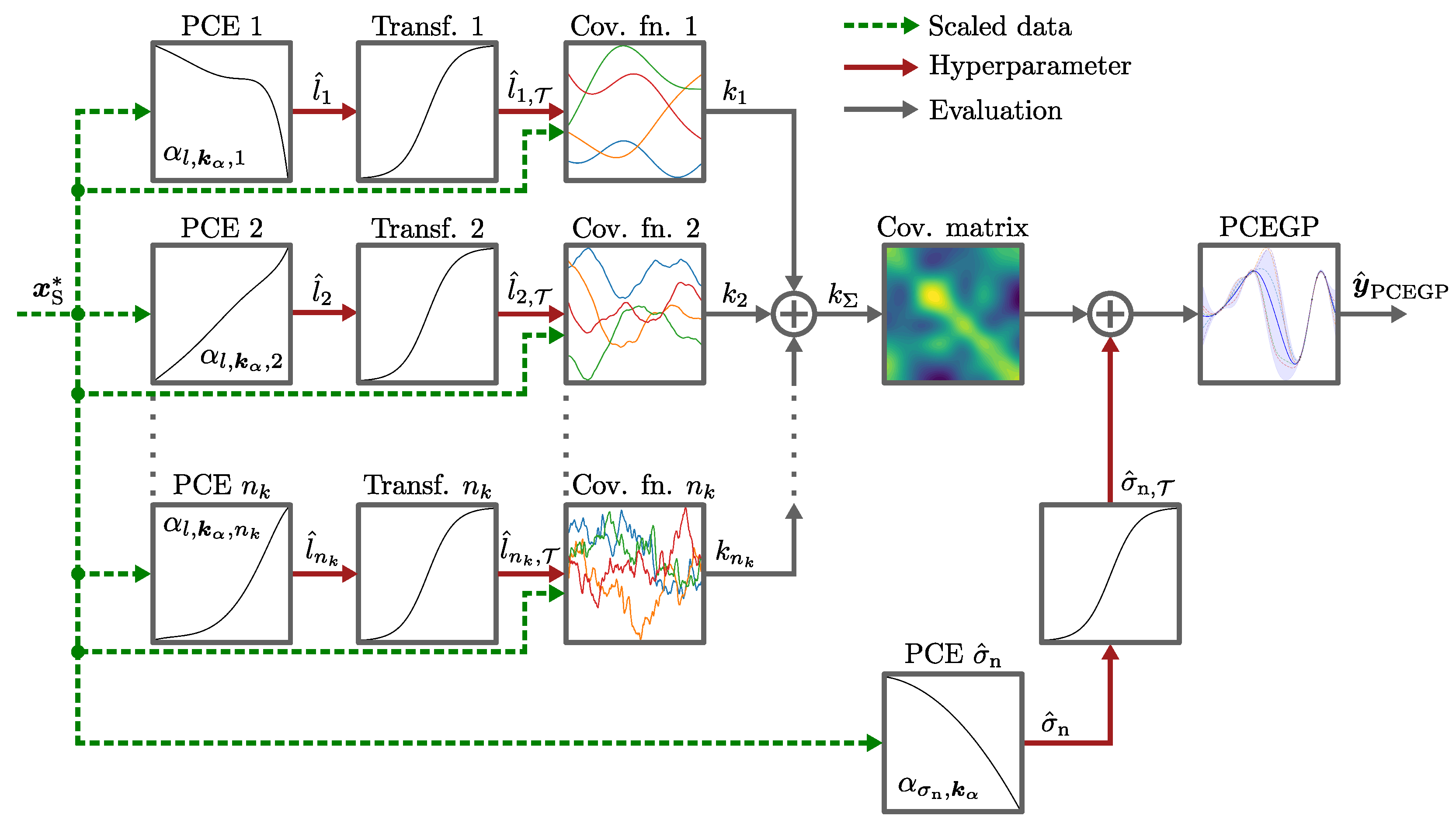
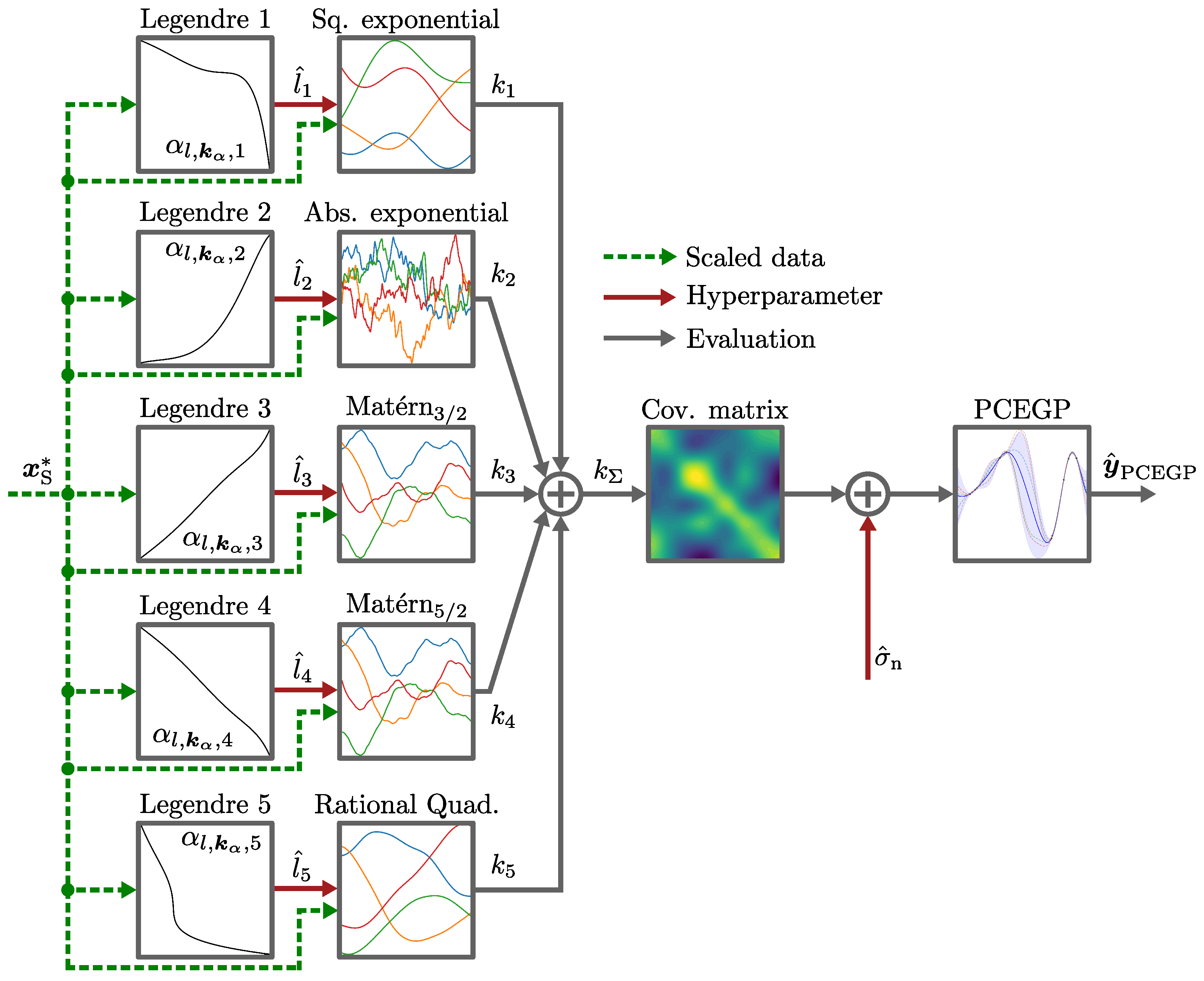
The general architecture of the PCEGP is shown in Figure 1. It consists of data scaling of the input ${\mathit{x}}^{*}$, data point-dependent hyperparameter calculation, and the prediction of the output ${\widehat{\mathit{y}}}_{\mathrm{PCEGP}}$ in ${\mathbb{R}}^2$, which includes the mean and uncertainty prediction. First, the given input data point ${\mathit{x}}^{*}$ is scaled to ${\mathit{x}}_{\mathrm{s}}^{*}$ with a scaler, e.g., the min–max scaler.

As illustrated in Figure 1, the scaled data point ${\mathit{x}}_{\mathrm{s}}^{*}$ is directly used as the input for the PCEs, which form the first processing stage after data scaling and are used to calculate the input-dependent hyperparameters of the GP. For each covariance function $k_1\dots k_{n_k}$, a separate PCE is used to predict the corresponding input-dependent lengthscale hyperparameters ${\widehat{l}}_1\left({\mathit{x}}_{\mathrm{s}}^{*}\right)\dots {\widehat{l}}_{n_k}\left({\mathit{x}}_{\mathrm{s}}^{*}\right)$, where $n_k\in \mathbb{N}$ denotes the number of used covariance functions. The scaled data point ${\mathit{x}}_{\mathrm{s}}^{*}$ is also used as the input for the PCE that calculates the input-dependent heteroscedastic noise parameter ${\widehat{\sigma }}_{\mathrm{n}}\left({\mathit{x}}_{\mathrm{s}}^{*}\right)$. The input-dependent lengthscale parameters ${\widehat{l}}_i\left({\mathit{x}}_{\mathrm{s}}^{*}\right)$ predicted by the PCE are transformed to ensure that the lengthscale ${\widehat{l}}_{i,\mathcal{T}}\left({\mathit{x}}_{\mathrm{s}}^{*}\right)$ is in ${\mathbb{R}}^{+}$. Similarly, the predicted input-dependent noise parameter ${\widehat{\sigma }}_{\mathrm{n}}\left({\mathit{x}}_{\mathrm{s}}^{*}\right)$ is transformed to ${\widehat{\sigma }}_{\mathrm{n},\mathcal{T}}\left({\mathit{x}}_{\mathrm{s}}^{*}\right)$ to ensure that it remains in ${\mathbb{R}}^{+}$.

The choice of the PCE basis function depends on the input data. The approach of this study allows the combination of different polynomial bases for the calculation of the GP hyperparameters depending on the input data. This eliminates the choice of the polynomial basis, and the weighting of these becomes part of the HPO. As shown in Figure 1, the combination of different PCE basis functions is achieved by a linear combination of these bases.

Non-stationary covariance functions enable the model to dynamically adjust to functions characterized by varying degrees of smoothness and training point densities across the input space. For GPs, this can be achieved by the estimation of an input-dependent lengthscale parameter $l\left(\mathit{x}\right)$ of a chosen covariance function. In this work, the PCE is used to calculate the lengthscale parameters as a function of the input data.

For this purpose, the stationary covariance functions have to be adapted to estimate a data point-dependent lengthscale $l\left(\mathit{x}\right)$. For example, the squared exponential covariance function

$$k\left(\mathit{x},{\mathit{x}}^{\prime }\right)={\sigma }_{\mathrm{f}}^2\exp \left(-{\displaystyle \frac{\parallel \mathit{x}-{\mathit{x}}^{\prime }{\parallel }^2}{2l^2}}\right),$$

(18)

is changed to

$$k\left(\mathit{x},{\mathit{x}}^{\prime }\right)={\sigma }_{\mathrm{f}}^2\exp \left(-{\displaystyle \frac{\parallel l\left(\mathit{x}\right)\mathit{x}-l\left({\mathit{x}}^{\prime }\right){\mathit{x}}^{\prime }{\parallel }^2}{2}}\right),$$

(19)

which enables the possibility to calculate the lengthscale for each data point separately by the PCE. This construction follows the approach in [5,12], where the input-dependent lengthscale is learned with a DNN. In the present work this mapping is parameterized by a PCE. This makes it possible to transform any stationary covariance function into a non-stationary one. Here, $l\left(\mathit{x}\right)$ is generally described as an input-dependent lengthscale. The lengthscale value calculated by the PCE is denoted with $\widehat{l}\left(\mathit{x}\right)$. In Figure 1, the case $\widehat{l}\left({\mathit{x}}_{\mathrm{s}}^{*}\right)$ is shown, where the data point ${\mathit{x}}_{\mathrm{s}}^{*}$ is already scaled.

To avoid problems with the covariance calculation, an output scaling by standardization is used in the following, which also corresponds to the previously mentioned assumption of $\mathit{y}\sim \mathcal{N}\left(0,\mathit{K}\left(\mathit{X},\mathit{X}\right)+{\sigma }_{\mathrm{n}}^2\mathit{I}\right)$ for the GP output.

The choice of the polynomial basis depends on the distribution of the input data. With

$$\widehat{l}\left(\mathit{x}\right)=\sum _{{\mathit{k}}_{\alpha }\in {\mathcal{K}}_{\alpha ,l}}{\alpha }_{l,{\mathit{k}}_{\alpha }}{\mathrm{\Phi }}_{{\mathit{k}}_{\alpha }}\left(\mathit{x}\right),$$

(20)

the lengthscale becomes an input-dependent hyperparameter for the covariance functions, estimated by the PCE. From this point onward, the optimizer’s task shifts from directly adjusting the lengthscale parameters to optimizing the $N_{l,\alpha }\in \mathbb{N}$ coefficients of the PCE for lengthscale calculation. In the case where the lengthscale parameter is calculated by a linear combination of b polynomial expansions, the number of parameters to optimize changes to

$$N_{l,\alpha }=b\left({\displaystyle \genfrac{}{}{0pt}{}{n_x+q_l}{q_l}}\right)=b{\displaystyle \frac{(n_x+q_l)!}{n_x!q_l!}},$$

(21)

where $q_l$ denotes the polynomial degree of the PCE for lengthscale estimation. The polynomial coefficients of the input-dependent lengthscale $\widehat{l}\left(\mathit{x}\right)$ are summarized in the vector ${\mathit{\alpha }}_l\in {\mathbb{R}}^{N_{l,\alpha }}$.

The superposition of the polynomial expansions is achieved by a linear combination of the polynomials, as demonstrated in Figure 1 with

$$\begin{array}{c}\hfill \widehat{l}\left(\mathit{x}\right)=\sum _{{\mathit{k}}_{\alpha }\in {\mathcal{K}}_{l,\alpha }}{\alpha }_{l,{\mathit{k}}_{\alpha ,1}}{\mathrm{\Phi }}_{{\mathit{k}}_{\alpha ,1}}\left(\mathit{x}\right)+\sum _{\mathit{k}\in {\mathcal{K}}_{l,\alpha }}{\alpha }_{l,{\mathit{k}}_{\alpha ,1}}{\mathrm{\Phi }}_{{\mathit{k}}_{\alpha ,2}}\left(\mathit{x}\right)+\cdots +\sum _{{\mathit{k}}_{\alpha }\in {\mathcal{K}}_{l,\alpha }}{\alpha }_{l,{\mathit{k}}_{\alpha ,b}}{\mathrm{\Phi }}_{{\mathit{k}}_{\alpha ,b}}\left(\mathit{x}\right).\end{array}$$

(22)

A separate PCE is also used to model the heteroscedastic noise parameter ${\widehat{\sigma }}_{\mathrm{n}}^2\left(\mathit{x}\right)$ of the GP as a function of the input data. The estimation of the noise parameter is defined by

$${\widehat{\sigma }}_{\mathrm{n}}^2\left(\mathit{x}\right)=\sum _{{\mathit{k}}_{\alpha }\in {\mathcal{K}}_{{\sigma }_{\mathrm{n}},\alpha }}{\alpha }_{{\sigma }_{\mathrm{n}},{\mathit{k}}_{\alpha }}{\mathrm{\Phi }}_{{\mathit{k}}_{\alpha }}\left(\mathit{x}\right).$$

(23)

Assuming the noise variance ${\sigma }_{\mathrm{n}}^2\left(\mathit{x}\right)$ of real sensor data depends on the measurement range but usually does not exhibit highly complex behavior, the polynomial degree can be truncated to a significantly smaller value $q_{{\sigma }_{\mathrm{n}}}$ than for the lengthscale calculation. This also limits the number of parameters $N_{{\sigma }_{\mathrm{n}},\alpha }\in \mathbb{N}$ to be optimized for modeling the noise variance

$$N_{{\sigma }_{\mathrm{n}},\alpha }=\left({\displaystyle \genfrac{}{}{0pt}{}{n_x+q_{{\sigma }_{\mathrm{n}}}}{q_{{\sigma }_{\mathrm{n}}}}}\right)={\displaystyle \frac{(n_x+q_{{\sigma }_{\mathrm{n}}})!}{n_x!q_{{\sigma }_{\mathrm{n}}}!}}.$$

(24)

The coefficients for noise estimation by the PCE are summarized in ${\mathit{\alpha }}_{{\sigma }_{\mathrm{n}}}\in {\mathbb{R}}^{N_{{\sigma }_{\mathrm{n}},\alpha }}$. In GP models, the lengthscale and noise parameters are critical in defining the covariance function that determines the covariance between input points. The lengthscale controls how quickly the correlation between data points decays with increasing distance, while the noise parameter represents the variance of the observed noise. For these hyperparameters to function correctly, they must satisfy certain constraints to ensure a valid covariance structure.

Ensuring that the lengthscale parameter $\widehat{l}\left(\mathit{x}\right)$ remains positive is essential as a non-positive lengthscale would violate the mathematical requirements for the GP. If the lengthscale is zero or negative, the covariance function may not properly represent the distance-dependent correlations between points, resulting in an invalid covariance matrix. A positive lengthscale ensures that the kernel function decreases smoothly as the distance between points increases, which is necessary to maintain a valid GP model and for the covariance matrix to remain positive semidefinite (PSD). This requirement means that for any non-trivial vector $\mathit{v}\in {\mathbb{R}}^N$, the condition

$${\mathit{v}}^{⊺}\mathit{K}(\mathit{X},\mathit{X})\mathit{v}\ge 0$$

(25)

must hold. Similarly, the noise variance ${\widehat{\sigma }}_{\mathrm{n}}^2\left(\mathit{x}\right)$ must be non-negative. The noise variance contributes to the diagonal elements of the covariance matrix. If ${\widehat{\sigma }}_{\mathrm{n}}^2\left(\mathit{x}\right)<0$, the diagonal elements of the covariance matrix may become negative, which would violate the requirement for positive semidefiniteness. Negative noise variances do not make sense in a probabilistic model as variances cannot be negative. Thus, ensuring that ${\widehat{\sigma }}_{\mathrm{n}}^2\left(\mathit{x}\right)\ge 0$ is crucial for maintaining the validity of the GP.

When using methods such as the PCE to estimate the lengthscale and noise variance of a GP, it is possible that the values generated may be zero or negative. The PCE can generate any real-valued output within its stochastic domain, including values that are not appropriate for parameters such as lengthscale and noise. A transformation is required to ensure that these hyperparameters satisfy the necessary constraints.

A transformation $\mathcal{T}$ is applied to map the estimated lengthscale $\widehat{l}\left(\mathit{x}\right)$ and noise ${\widehat{\sigma }}_{\mathrm{n}}^2\left(\mathit{x}\right)$ to valid domains

$${\widehat{l}}_{\mathcal{T}}\left(\mathit{x}\right)=\mathcal{T}\left(\widehat{l}\left(\mathit{x}\right)\right),{\widehat{\sigma }}_{\mathrm{n},\mathcal{T}}^2\left(\mathit{x}\right)=\mathcal{T}\left({\widehat{\sigma }}_{\mathrm{n}}^2\left(\mathit{x}\right)\right).$$

(26)

In this setting, $\widehat{l}\left(\mathit{x}\right)$ and ${\widehat{\sigma }}_{\mathrm{n}}^2\left(\mathit{x}\right)$ denote unconstrained PCE outputs, whereas the GP covariance function is evaluated only with the transformed quantities ${\widehat{l}}_{\mathcal{T}}\left(\mathit{x}\right)$ and ${\widehat{\sigma }}_{\mathrm{n},\mathcal{T}}^2\left(\mathit{x}\right)$. The resulting covariance matrix element of input ${\mathit{x}}_i$ and ${\mathit{x}}_j$ can be written as

$$K_{ij}=k\left({\mathit{x}}_i,{\mathit{x}}_j;{\widehat{l}}_{\mathcal{T}}\right)+{\delta }_{ij}{\widehat{\sigma }}_{\mathrm{n},\mathcal{T}}^2\left({\mathit{x}}_i\right),$$

(27)

so that only strictly positive lengthscales and noise variances enter the kernel.

A common choice for such a transformation is the softplus transformation, which maps any real number to ${\mathbb{R}}^{+}$. The softplus transformation is defined as

$${\widehat{l}}_{\mathcal{T}}\left(\mathit{x}\right)=\log \left(1+{\mathrm{e}}^{\widehat{l}\left(\mathit{x}\right)}\right)\mathrm{and}{\widehat{\sigma }}_{\mathrm{n},\mathcal{T}}^2\left(\mathit{x}\right)=\log \left(1+{\mathrm{e}}^{{\widehat{\sigma }}_{\mathrm{n}}^2\left(\mathit{x}\right)}\right).$$

(28)

By applying this approach, both the lengthscale and the noise remain positive during the HPO process.

To perform versatile modeling tasks with this novel approach, different covariance functions are combined, and the influence of the respective covariance function is controlled by HPO. The combination of the covariance functions is realized by summation of the covariance functions with

$$k_{\sum }\left(\mathit{x},{\mathit{x}}^{\prime }\right)=k_1\left(\mathit{x},{\mathit{x}}^{\prime }\right)+k_2\left(\mathit{x},{\mathit{x}}^{\prime }\right)+\cdots +k_{n_k}\left(\mathit{x},{\mathit{x}}^{\prime }\right).$$

(29)

The covariance matrix is then computed from the combined covariance function, and the prediction ${\widehat{\mathit{y}}}_{\mathrm{PCEGP},\mathrm{s}}$ is determined by combining this matrix with the estimated noise. Finally, the predictions are rescaled to the original range ${\widehat{\mathit{y}}}_{\mathrm{PCEGP}}$. In Algorithm 1, the algorithm for model prediction is shown. In this work, the covariance functions and polynomial bases are chosen manually and are not part of the HPO. In Section 5, the setup of the model for the experiments carried out in this work is presented in detail.

Algorithm 1 PCEGP model prediction

Input: Input data ${\mathit{x}}^{*}$ Output: Model prediction ${\widehat{\mathit{y}}}_{\mathrm{PCEGP}}$ Specified in the model: Covariance functions $k_1\left(\mathit{x},{\mathit{x}}^{\prime }\right),\dots ,k_{n_k}\left(\mathit{x},{\mathit{x}}^{\prime }\right)$, combined covariance function $k_{\Sigma }\left(\mathit{x},{\mathit{x}}^{\prime }\right)$, polynomials for lengthscale ${\widehat{l}}_i\left(\mathit{x}\right)$, polynomials for noise variance ${\widehat{\sigma }}_{\mathrm{n}}^2\left(\mathit{x}\right)$, transformation $\mathcal{T}$, transformed hyperparameters ${\widehat{\mathit{l}}}_{\mathcal{T}}\left({\mathit{X}}_{\mathrm{s}}\right)$ and ${\widehat{\sigma }}_{\mathrm{n},\mathcal{T}}^2\left({\mathit{X}}_{\mathrm{s}}\right)$ at the training inputs, covariance matrix $\mathit{K}\left({\mathit{X}}_{\mathrm{s}},{\mathit{X}}_{\mathrm{s}}\right)+{\widehat{\sigma }}_{\mathrm{n},\mathcal{T}}^2\left({\mathit{X}}_{\mathrm{s}}\right)\mathit{I}$ depending on the training data, and model hyperparameters ${\mathit{\theta }}_{\mathrm{PCEGP}}$   1: Step 1: Scale input and output data:   2: ${\mathit{x}}_{\mathrm{s}}^{*}\leftarrow \mathrm{Scale}\mathrm{input}\mathrm{data}{\mathit{x}}^{*}$   3: Step 2: Calculate the point-dependent lengthscale (PCE output):   4: for $i=1\dots n_k$ do   5:       ${\widehat{l}}_i\left({\mathit{x}}_{\mathrm{s}}^{*}\right)\leftarrow {\sum }_{\mathit{k}\in {\mathcal{K}}_l}{\alpha }_{l,i,\mathit{k}}{\mathrm{\Phi }}_{\mathit{k}}\left({\mathit{x}}_{\mathrm{s}}^{*}\right)$   6: end for   7: Step 3: Transform the point-dependent lengthscale:   8: for $i=1\dots n_k$ do   9:       ${\widehat{l}}_{i,\mathcal{T}}\left({\mathit{x}}_{\mathrm{s}}^{*}\right)\leftarrow \mathcal{T}\left({\widehat{l}}_i\left({\mathit{x}}_{\mathrm{s}}^{*}\right)\right)$ 10: end for 11: Step 4: Calculate point-dependent covariance for each training point and kernel, and sum to $k_{\Sigma }$: 12: for $j=1\dots N$ do 13:       $k_{\Sigma }({\mathit{x}}_{\mathrm{s},j},{\mathit{x}}_{\mathrm{s}}^{*})\leftarrow 0$ 14:       for $i=1\dots n_k$ do 15:             $k_i({\mathit{x}}_{\mathrm{s},j},{\mathit{x}}_{\mathrm{s}}^{*})\leftarrow ∥{\widehat{l}}_{i,\mathcal{T}}\left({\mathit{x}}_{\mathrm{s},j}\right){\mathit{x}}_{\mathrm{s},j}-{\widehat{l}}_{i,\mathcal{T}}\left({\mathit{x}}_{\mathrm{s}}^{*}\right){\mathit{x}}_{\mathrm{s}}^{*}∥$ 16:             $k_{\Sigma }({\mathit{x}}_{\mathrm{s},j},{\mathit{x}}_{\mathrm{s}}^{*})\leftarrow k_{\Sigma }({\mathit{x}}_{\mathrm{s},j},{\mathit{x}}_{\mathrm{s}}^{*})+k_i({\mathit{x}}_{\mathrm{s},j},{\mathit{x}}_{\mathrm{s}}^{*})$ 17:       end for 18: end for 19: Step 5: Summarize covariances into a vector: 20: ${\mathit{k}}_{\Sigma }\left({\mathit{X}}_{\mathrm{s}},{\mathit{x}}_{\mathrm{s}}^{*}\right)\leftarrow {\left[k_{\Sigma }({\mathit{x}}_{\mathrm{s},1},{\mathit{x}}_{\mathrm{s}}^{*}),\dots ,k_{\Sigma }({\mathit{x}}_{\mathrm{s},N},{\mathit{x}}_{\mathrm{s}}^{*})\right]}^{⊺}$ 21: Step 6: Compute point-dependent noise variance (PCE output): 22: ${\widehat{\sigma }}_{\mathrm{n}}^2\left({\mathit{x}}_{\mathrm{s}}^{*}\right)\leftarrow {\sum }_{\mathit{k}\in {\mathcal{K}}_{{\sigma }_{\mathrm{n}}}}{\alpha }_{{\sigma }_{\mathrm{n}},\mathit{k}}{\mathrm{\Phi }}_{\mathit{k}}\left({\mathit{x}}_{\mathrm{s}}^{*}\right)$ 23: Step 7: Transform the point-dependent noise variance: 24: ${\widehat{\sigma }}_{\mathrm{n},\mathcal{T}}^2\left({\mathit{x}}_{\mathrm{s}}^{*}\right)\leftarrow \mathcal{T}\left({\widehat{\sigma }}_{\mathrm{n}}^2\left({\mathit{x}}_{\mathrm{s}}^{*}\right)\right)$ 25: Step 8: Compute scaled output mean: 26: ${\widehat{y}}_{\mathrm{PCEGP},\mathrm{s},\mathrm{m}}\leftarrow {\widehat{m}}_{\mathrm{s}}\left({\mathit{x}}_{\mathrm{s}}^{*}\right)+{\mathit{k}}_{\Sigma }{\left({\mathit{X}}_{\mathrm{s}},{\mathit{x}}_{\mathrm{s}}^{*}\right)}^{⊺}{\left(\mathit{K}\left({\mathit{X}}_{\mathrm{s}},{\mathit{X}}_{\mathrm{s}}\right)+{\widehat{\sigma }}_{\mathrm{n},\mathcal{T}}^2\left({\mathit{X}}_{\mathrm{s}}\right)\mathit{I}\right)}^{-1}\left(\mathit{y}-{\widehat{\mathit{m}}}_{\mathrm{s}}\left({\mathit{X}}_{\mathrm{s}}\right)\right)$ 27: Step 9: Compute scaled output variance: 28: ${\widehat{y}}_{\mathrm{PCEGP},\mathrm{s},\mathrm{v}}\leftarrow k_{\Sigma }\left({\mathit{x}}_{\mathrm{s}}^{*},{\mathit{x}}_{\mathrm{s}}^{*}\right)+{\widehat{\sigma }}_{\mathrm{n},\mathcal{T}}^2\left({\mathit{x}}_{\mathrm{s}}^{*}\right)-{\mathit{k}}_{\Sigma }{\left({\mathit{X}}_{\mathrm{s}},{\mathit{x}}_{\mathrm{s}}^{*}\right)}^{⊺}{\left(\mathit{K}\left({\mathit{X}}_{\mathrm{s}},{\mathit{X}}_{\mathrm{s}}\right)+{\widehat{\sigma }}_{\mathrm{n},\mathcal{T}}^2\left({\mathit{X}}_{\mathrm{s}}\right)\mathit{I}\right)}^{-1}{\mathit{k}}_{\Sigma }\left({\mathit{X}}_{\mathrm{s}},{\mathit{x}}_{\mathrm{s}}^{*}\right)$ 29: Step 10: Rescale the output: 30: ${\widehat{\mathit{y}}}_{\mathrm{PCEGP}}\leftarrow \mathrm{Rescale}\mathrm{the}\mathrm{output}{\widehat{\mathit{y}}}_{\mathrm{PCEGP},\mathrm{s}}\mathrm{of}\mathrm{the}\mathrm{PCEGP}\mathrm{model}$

3.2. Hyperparameter Optimization

In this work, HPO was performed with the tree-structured Parzen estimator (TPE) [33] and the Nadam optimizer. The Nadam optimizer combines the adaptive learning rate strategy of Adam [34] with the Nesterov momentum and is introduced in [35]. The Nadam optimizer is preferred over the Adam optimizer because it achieves faster convergence through the Nesterov momentum, as described in [35], making it particularly suitable given the large number of PCE coefficients in the model. This optimizer is well suited for the PCEGP approach since the log-marginal likelihood of the model is non-convex, the number of trainable PCE coefficients for the non-stationary lengthscale, and the noise can be large.

In the proposed PCEGP model, the PCE is not trained separately and then combined with the Gaussian process afterwards. Instead, the PCE coefficients directly parameterize the input-dependent GP hyperparameters, in particular the non-stationary lengthscale and, if used, the heteroscedastic noise. These coefficients are therefore optimized jointly within the GP training procedure through the model loss based on the log-marginal likelihood. Consequently, the optimization is carried out with respect to the PCEGP parameter vector as a whole, rather than through separate optimization problems for the PCE and the GP. Adaptive learning rates reduce the need for manual step-size tuning across differently scaled coefficients, and the momentum term stabilizes the optimization in narrow valleys of the objective. On the outer level, a Bayesian hyperparameter search based on the TPE treats Nadam as a black-box inner optimizer and searches over all hyperparameters that are not directly learned by gradient descent. A schematic overview of the optimization loop is given in Algorithm 2. The first step is to investigate the data for the choice of a suitable input and output scaler, covariance functions, and polynomial bases. After that, the data are scaled. A termination criterion has to be selected for the optimization loop, i.e., the number of trials for hyperparameter optimization. Then, the hyperparameter optimization starts with the TPE as a Bayesian approach. First, initial hyperparameter combinations are placed with random search in the entire hyperparameter space. Afterwards, new hyperparameters are suggested via the TPE algorithm.

For the TPE, the objective function for hyperparameter optimization takes the hyperparameters of the model as inputs. This includes the selection of the polynomial degree $q_l$ for the lengthscale $\widehat{l}\left(\mathit{x}\right)$ and the polynomial degree $q_{{\sigma }_{\mathrm{n}}}$ for the heteroscedastic noise variance ${\widehat{\sigma }}_{\mathrm{n}}^2\left(\mathit{x}\right)$ calculation. In addition, the scaling factors $\mathit{ϵ}$, the learning rate $\eta$, the number of gradient iterations $n_{\mathrm{I}}$, and the initial values of the PCE coefficients ${\mathit{\alpha }}_0$ are suggested via the TPE. In the case that elastic net regularization is used, the regularization parameters $\beta$ and $\lambda$ are also used as hyperparameters for the Bayesian optimization. The hyperparameter space of the PCEGP therefore contains both continuous and discrete variables, such as learning rates, scaling factors, and polynomial degrees, which can be handled in a unified way by the TPE. The model loss serves as the objective function and is minimized during hyperparameter optimization. In this process, the trainable PCE coefficients are updated jointly with the remaining model parameters, where they directly determine the input-dependent GP hyperparameters entering the covariance matrix. A shuffled k-fold cross-validation is used to evaluate this loss, where k different models are trained with a gradient descent method and the hyperparameters of the PCEGP are updated over $n_{\mathrm{I}}$ iterations.

In this work, Bayesian hyperparameter optimization based on the TPE ensures that the gradient descent procedure was performed with informative hyperparameter combinations. In contrast to grid search or pure random search, the TPE learns from poor hyperparameter combinations and reduces the probability of sampling new candidates in these regions. This property is particularly useful in the present setting since each trial is computationally expensive due to cross-validation and multiple gradient descent iterations, and a large part of the hyperparameter space corresponds to clearly suboptimal settings.

During gradient-based model hyperparameter optimization, the covariance matrix depends on the lengthscale PCE coefficients ${\mathit{\alpha }}_l$ and the noise PCE coefficients ${\mathit{\alpha }}_{{\sigma }_{\mathrm{n}}}$ and is described by

$$\begin{array}{c}\hfill \mathit{K}\left(\mathit{X},\mathit{X}\right)=\mathit{K}\left(\mathit{X},\mathit{X}\right)+{\widehat{\sigma }}_{\mathrm{n}}^2\left(\mathit{X}\right)\mathit{I}.\end{array}$$

(30)

Here, $\widehat{\mathit{l}}\left(\mathit{X}\right)\in {\mathbb{R}}^N$ denotes the prediction of the lengthscale parameters for each data point, obtained from the PCE as a function of the coefficients ${\mathit{\alpha }}_l$ and the input $\mathit{X}$. These input-dependent lengthscales enter the covariance function and, together with the remaining kernel hyperparameters, parameterize the non-stationary covariance matrix $\mathit{K}\left(\mathit{X},\mathit{X}\right)$. With ${\widehat{\sigma }}_{\mathrm{n}}^2\left(\mathit{X}\right)\in {\mathbb{R}}^N$, the prediction of the heteroscedastic noise, depending on the PCE coefficients ${\mathit{\alpha }}_{{\sigma }_{\mathrm{n}}}$ and the input $\mathit{X}$, is denoted and contributes to the diagonal term ${\widehat{\sigma }}_{\mathrm{n}}^2\left(\mathit{X}\right)\mathit{I}$. The task of the optimizer therefore shifts from optimizing the lengthscale and noise directly to optimizing the polynomial coefficients of the PCE. The gradient from Equation (15) is evaluated with respect to these polynomial coefficients for hyperparameter optimization.

Algorithm 2 Hyperparameter optimization of PCEGP model

Input: Data $\mathcal{D}=\{\mathit{X},\mathit{y}\}$, number of trials $n_{\mathrm{T}}$, number of initial trials $n_{\mathrm{IT}}$, number of folds $n_{\mathrm{F}}$, number of gradient descent iterations $n_{\mathrm{I}}$ Output: Optimized model hyperparameters ${\mathit{\theta }}_{\mathrm{PCEGP}}={\left[\begin{array}{ccccc}{q}_l& q_{{\sigma }_{\mathrm{n}}}& {\mathit{\alpha }}_l^{⊺}& {\mathit{\alpha }}_{{\sigma }_{\mathrm{n}}}^{⊺}& {\sigma }_{\mathrm{f}}^2\end{array}\right]}^{⊺}$ and training hyperparameters $\eta$, $n_{\mathrm{I}}$, $\beta$, $\lambda$, $\mathit{ϵ}$ Specified: Covariance function $k_{\Sigma }\left(\mathit{x},{\mathit{x}}^{\prime }\right)$, polynomials for lengthscale ${\widehat{l}}_i\left(\mathit{x}\right)$ and noise variance ${\widehat{\sigma }}_{\mathrm{n}}^2\left(\mathit{x}\right)$   1: repeat   2:     Step 1: Suggest hyperparameters:   3:     if $trial\le n_{\mathrm{IT}}$ then   4:           Random Search for $q_l$, $q_{{\sigma }_{\mathrm{n}}}$, $\eta$, $n_{\mathrm{I}}$, $\lambda$, $\mathit{ϵ}$   5:     else   6:           TPE for $q_l$, $q_{{\sigma }_{\mathrm{n}}}$, $\eta$, $n_{\mathrm{I}}$, $\lambda$, $\mathit{ϵ}$   7:     end if   8:     Step 2: Data scaling:   9:     ${\mathit{X}}_{\mathrm{s}},{\mathit{y}}_{\mathrm{s}}\leftarrow \mathrm{Scale}\mathrm{input}\mathrm{and}\mathrm{output}\mathrm{data}\mathit{X},\mathit{y}$ with scaling parameters $\mathit{ϵ}$ on ${\mathcal{D}}_{\mathrm{train}}$ 10:     for $fold=1\dots n_{\mathrm{F}}$ do 11:           Step 3: Cross-validation data split: 12:           ${\mathcal{D}}_{\mathrm{train}},{\mathcal{D}}_{\mathrm{val}}\leftarrow k-\mathrm{fold}\mathrm{split}\mathrm{of}\mathrm{data}\mathcal{D}$. 13:           Step 4: Setup PCEGP Model: 14:           Define covariance function $k_{\Sigma }\left(\mathit{x},{\mathit{x}}^{\prime }\right)$, polynomials ${\widehat{l}}_i\left(\mathit{x}\right)$ and ${\widehat{\sigma }}_{\mathrm{n}}^2\left(\mathit{x}\right)$ 15:           Step 5: Optimize model parameters on training data 16:           for $i=1\dots N_{\mathrm{I}}$ do 17:                Compute gradient: ${\mathit{g}}_i\leftarrow {\nabla }_{{\mathit{\theta }}_{\mathrm{PCEGP}}}\mathcal{L}\left({\mathit{\theta }}_{\mathrm{PCEGP},i-1}\right)$ 18:                Update first moment estimate: 19:                $m_i\leftarrow {\kappa }_i{m}_{i-1}+(1-{\kappa }_i)g_i$ 20:                Update second moment estimate: 21:                $v_i\leftarrow \nu v_{i-1}+(1-\nu )g_i^2$ 22:                Compute bias-corrected estimates: 23:           24:                ${\widehat{m}}_i\leftarrow {\displaystyle \frac{{\kappa }_{i+1}{m}_i}{1-{\prod }_{j=1}^{i+1}{\kappa }_j}}+{\displaystyle \frac{(1-{\kappa }_i)g_i}{1-{\prod }_{j=1}^i{\kappa }_j}}$, ${\widehat{v}}_i\leftarrow {\displaystyle \frac{v_i}{1-{\nu }^i}}$ 25:                Update parameters: ${\mathit{\theta }}_{\mathrm{PCEGP},i}\leftarrow {\mathit{\theta }}_{\mathrm{PCEGP},i-1}-{\displaystyle \frac{\eta }{\sqrt{{\widehat{v}}_i}+\zeta }}{\widehat{m}}_i$ 26:           end for 27:           Step 6: Compute validation loss: ${\mathcal{L}}_{\mathrm{val}}\left({\mathit{\theta }}_{\mathrm{PCEGP}},{\mathcal{D}}_{\mathrm{val}}\right)$ 28:     end for 29:     Step 7: Compute average loss across folds: 30:     ${\overline{\mathcal{L}}}_{\mathrm{val}}\leftarrow {\displaystyle \frac{1}{n_{\mathrm{F}}}}{\sum }_{fold=1}^{n_{\mathrm{F}}}{\mathcal{L}}_{\mathrm{val}}\left({\mathit{\theta }}_{\mathrm{PCEGP}},{\mathcal{D}}_{\mathrm{val}}\right)$ 31:     Step 8: Update best model and training hyperparameters: 32:     if ${\overline{\mathcal{L}}}_{\mathrm{val}}<{\overline{\mathcal{L}}}_{\mathrm{val},\mathrm{best}}$ then 33:           ${\mathit{\theta }}_{\mathrm{PCEGP},\mathrm{best}}\leftarrow {\mathit{\theta }}_{\mathrm{PCEGP}}$ 34:           ${\eta }_{\mathrm{best}},n_{\mathrm{I},\mathrm{best}},{\lambda }_{\mathrm{best}},{\mathit{ϵ}}_{\mathrm{best}}\leftarrow \eta ,n_{\mathrm{I}},\lambda ,\mathit{ϵ}$ 35:     end if 36:     $trial\leftarrow trial+1$ 37: until $trial=n_{\mathrm{T}}$

3.3. Time Complexity of the PCEGP Algorithm

In this section, the time complexity of the proposed ML approach is analyzed. The analysis covers two main aspects, namely, the time complexity of the training process, which entails fitting the model to the data, and the time complexity of the prediction process, which requires making predictions using the trained model. The following subsections provide detailed explanations of these two components. In addition, the runtime of the PCEGP implementation in the Python 3.8.18 framework is analyzed experimentally and compared to a standard GP implementation in GPyTorch 1.11.

3.3.1. Time Complexity for Training

The time complexity of the PCEGP algorithm is composed of several components, each representing different aspects of the training process. First, the time complexity of the standard GP is examined, followed by an introduction to the PCE component, and finally the combined PCEGP time complexity.

For the GP, the time complexity arises from two main computational steps. The first step involves the computation of the covariance matrix between all training points, which depends on the number of training points N. The covariance matrix $\mathit{K}\left(\mathit{X},\mathit{X}\right)$ requires a constant number of operations for each entry, resulting in a time complexity of $\mathcal{O}\left(N^2\right)$ for this step [1]. The next step is the Cholesky factorization of the covariance matrix, which is required to make predictions and to compute the LML of the model for optimizing the hyperparameters. This step has a time complexity of $\mathcal{O}\left(N^3\right)$ and scales cubically with the number of training points N. The dominant term in the time complexity of the standard GP is $\mathcal{O}\left(N^3\right)$ [1].

In contrast, PCE time complexity is defined by the evaluation and calculation of the polynomial terms. Before the training process begins, the polynomial values for the PCE are precomputed and remain constant throughout the entire training phase. For the PCE itself, the PCE coefficients are multiplied by the corresponding polynomial values and then summed for each training point. The number of multiplications is therefore the product of the number of PCE coefficients $N_{\alpha }$ and the number of training points N, which leads to a complexity of $\mathcal{O}\left(N{N}_{\alpha }\right)$ for this step. In classical Big-O notation it is common practice to omit constant factors and to treat model-size parameters such as $N_{\alpha }$ as fixed. However, in this work $N_{\alpha }$ can become very large, and configurations with $N\ll N_{\alpha }$ occur. Therefore, the dependence on both N and $N_{\alpha }$ is made explicit in the term $\mathcal{O}\left(N{N}_{\alpha }\right)$.

The combined time complexity of the PCEGP algorithm is obtained by adding the GP complexity $\mathcal{O}(N^2+N^3)$ to the PCE complexity $\mathcal{O}\left(N{N}_{\alpha }\right)$. In this combined view, the cubic term $\mathcal{O}\left(N^3\right)$, arising from the GP, dominates for sufficiently large N, while for small N and very large $N_{\alpha }$ the PCE term can become relevant. The per-iteration training complexity of the PCEGP can be summarized as

$$T_{\mathrm{PCEGP},\mathrm{train}}(N,N_{\alpha })=\mathcal{O}\left(N^3+N{N}_{\alpha }\right).$$

(31)

For comparison, the per-iteration training time complexity of a standard GP can be written as

$$T_{\mathrm{GP},\mathrm{train}}\left(N\right)=\mathcal{O}\left(N^3\right).$$

(32)

This analytical comparison shows that the PCEGP has the same cubic scaling in N as a standard GP and adds an additional term of order $\mathcal{O}\left(N{N}_{\alpha }\right)$, which represents the cost of evaluating the PCE-based hyperparameters.

The crossover between both regimes can be understood by comparing the two terms. A rough crossover point is obtained by equating the contributions of the two terms

$$N^3=N{N}_{\alpha },$$

(33)

which yields

$$N^2=N_{\alpha }\Rightarrow N=\sqrt{N_{\alpha }}.$$

(34)

For $N\gg \sqrt{N_{\alpha }}$, the cubic term dominates and the training complexity of the PCEGP is asymptotically equivalent to that of a standard GP as $T_{\mathrm{PCEGP},\mathrm{train}}(N,N_{\alpha })=\mathcal{O}\left(N^3\right)$ for fixed $N_{\alpha }$. For theoretical analysis, the time complexity of the PCEGP for different $N_{\alpha }$ is compared with the time complexity of the standard GP and analyzed as a function of N. In Figure 2, the theoretical training and prediction time complexity of the GP and PCEGP is illustrated. The left-hand subplot shows the training complexity for different $N_{\alpha }$. It can be observed that $N_{\alpha }$ has a significant impact on the runtime for small datasets. For $N\approx 10$, the difference between 120 and 11,440 coefficients in the PCEGP is clearly visible. As N increases, the cubic growth rate of the GP part dominates the scaling, and the curves for the PCEGP and GP become nearly parallel when both axes are plotted on a logarithmic scale. The influence of $N_{\alpha }$ is primarily reflected in a vertical offset between the curves rather than in a different asymptotic order.

3.3.2. Time Complexity for Prediction

The time complexity of the PCEGP during the evaluation or prediction phase is composed of two distinct components that contribute to the overall complexity. The first component represents the time complexity to apply the trained GP for making predictions. After training, the Cholesky factor of $\mathit{K}(\mathit{X},\mathit{X})$ and the vector ${\mathit{\alpha }}_{\mathrm{Cholesky}}=\mathit{K}{(\mathit{X},\mathit{X})}^{-1}\mathit{y}$ are available. For a standard GP, computing the predictive mean and variance for M test points requires $\mathcal{O}\left(M{N}^2\right)$ operations in total, dominated by triangular solves and matrix–vector multiplications [1]. Thus, the prediction complexity of a standard GP is

$$T_{\mathrm{GP},\mathrm{pred}}(N,M)=\mathcal{O}\left(M{N}^2\right).$$

(35)

The second component in the PCEGP arises from the computation of the PCE polynomial values at the evaluation points. For each of the M test points, the PCE is evaluated as a linear combination of $N_{\alpha }$ basis functions, which requires $\mathcal{O}\left(N_{\alpha }\right)$ operations per test point. For M test points, this contribution scales as $\mathcal{O}\left(M{N}_{\alpha }\right)$. Combining these two components, the total prediction complexity of the PCEGP becomes

$$T_{\mathrm{PCEGP},\mathrm{pred}}(N,N_{\alpha },M)=\mathcal{O}\left(M(N^2+N_{\alpha })\right).$$

(36)

Again, the crossover between both regimes can be seen by comparing the two terms. A crossover point is obtained by equating

$$N^2=N_{\alpha },$$

(37)

which yields

$$N=\sqrt{N_{\alpha }}.$$

(38)

For $N\gg \sqrt{N_{\alpha }}$, the quadratic term in N dominates, and the prediction complexity is asymptotically equivalent to that of a standard GP, that is, $\mathcal{O}\left(N^2\right)$ in N for fixed M. For small N and large $N_{\alpha }$, the PCE evaluation dominates, which leads to an almost constant runtime in N that scales linearly with $N_{\alpha }$.

In Figure 2, the theoretical training and prediction time complexity of the GP and PCEGP are illustrated as a function of the number of training points N. The right-hand subplot displays the prediction complexity for a fixed number of test points M and shows the increasing influence of $N_{\alpha }$ for small N, followed by convergence towards the GP scaling as N grows.

3.4. Runtime Comparison of PCEGP and GP

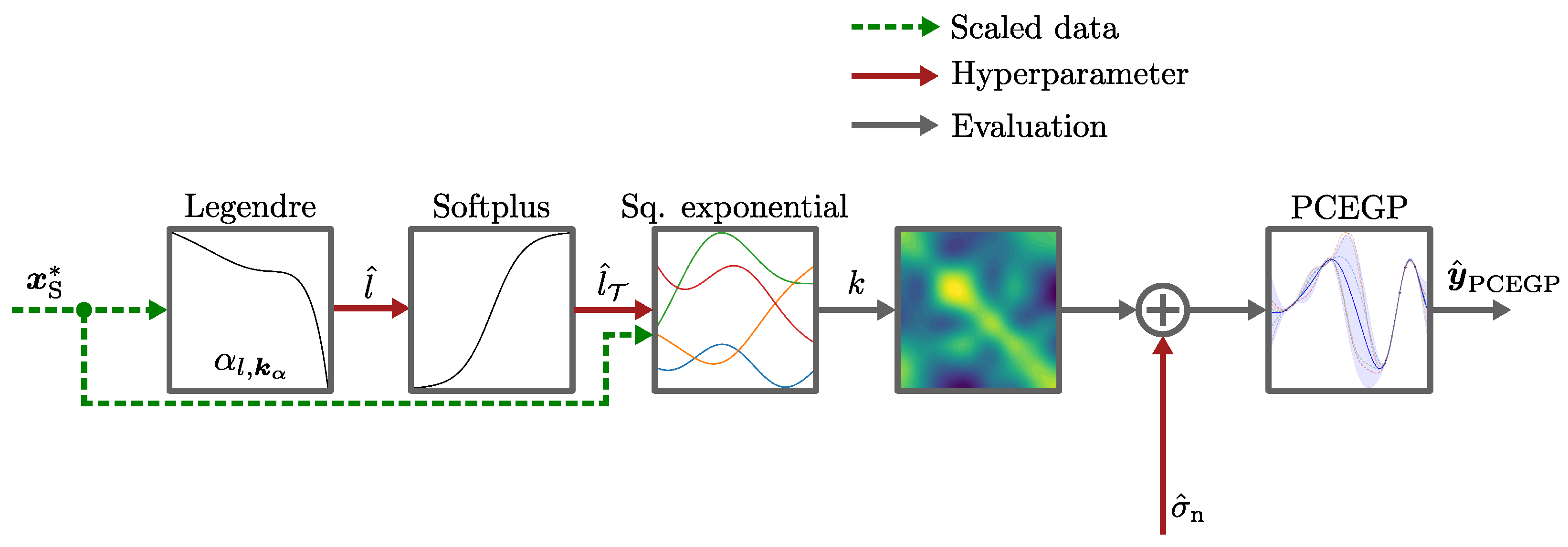
In this section, a runtime comparison between the standard GP from GPyTorch [36] and the PCEGP is presented. Three scenarios with $N_{\alpha }\approx 100$, $N_{\alpha }\approx$ 1000, and $N_{\alpha }\approx$ 10,000 for the PCEGP were generated, where three different PCEs were used. For all experiments of the runtime comparison, the squared exponential covariance function was used. The non-stationary lengthscale parameters were calculated with a Legendre polynomial and a uniform distribution in $\left[-1,1\right]$.

The first configuration was implemented with $n_x=7$ and $q_l=3$, resulting in $N_{\alpha }=120$. To achieve $N_{\alpha }=1001$, a configuration with $n_x=10$ and $q_l=4$ was employed. The third configuration was implemented with $n_x=9$ and $q_l=7$, which resulted in $N_{\alpha }=$ 11,440. For the standard GP, the model training and predictions were performed with $n_x=7$. For all inputs, equidistantly spaced data between 0 and 1 were generated. The output was the simple test function $\tanh \left(\mathit{x}\right)$, where $\mathit{x}$ was generated by summarizing each input $x_i$. The experiments were carried out for $N=10$ up to $N=5000$ with a step size of 50. All experiments were repeated ten times for statistical validation. Each model was trained over 100 gradient descent iterations, with the training time averaged per iteration. The prediction times were calculated by averaging the time required to make predictions for $M=100$ test data points. The PCEGP model was implemented using the base elements of the GPyTorch library 1.11 for kernel implementations and the SciPy library 1.10.1 [37] for the implementation of the PCE. The standard GP was implemented using the GPyTorch library. The experiments were conducted on a QEMU virtual CPU with 64 virtual CPUs, 32 GB of RAM, and a clock speed of 2.50 GHz. 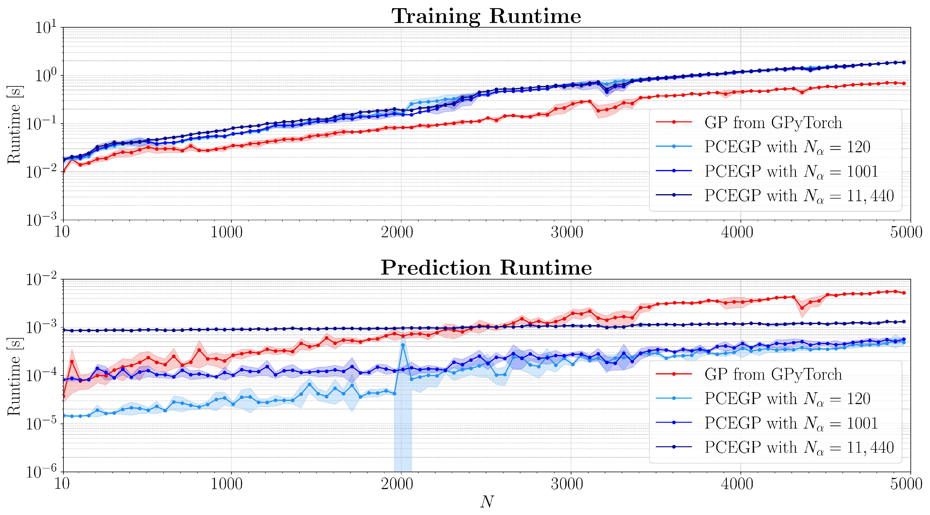In Figure 3, the runtime comparison for training and prediction of the PCEGP and GP is illustrated. The PCEGP approach exhibits training runtimes slightly above the standard GP from GPyTorch per gradient descent iteration. 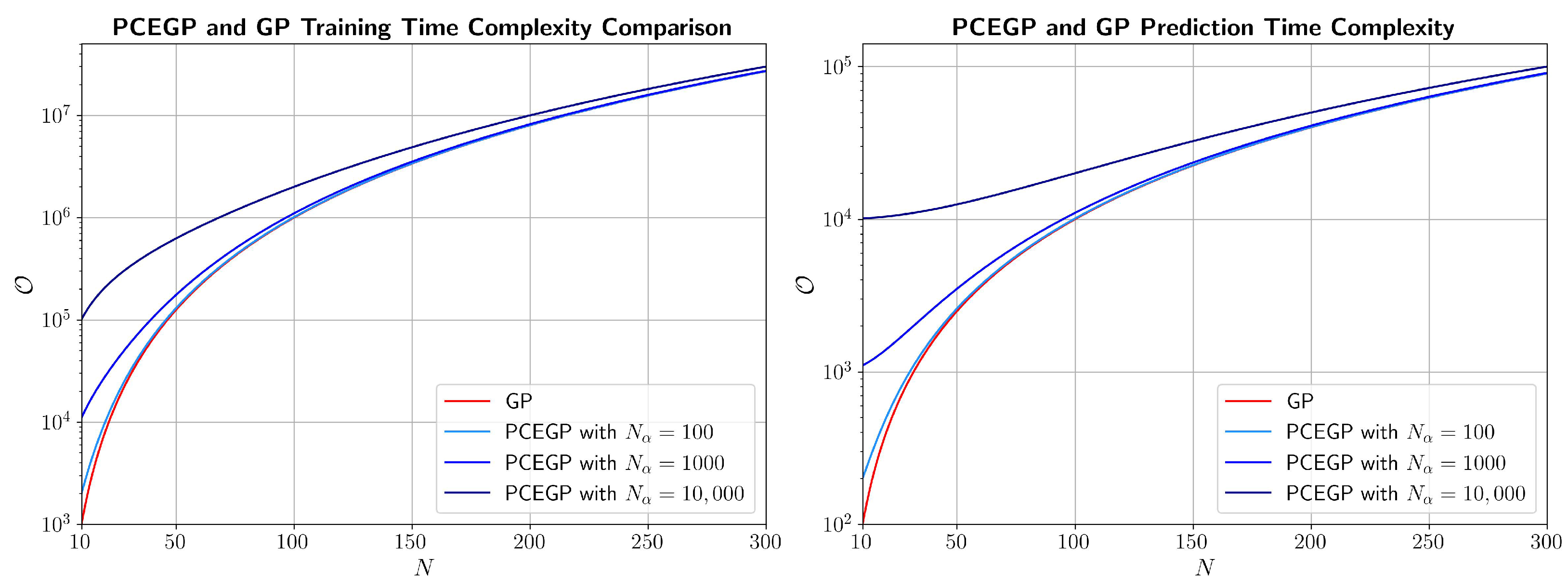This behavior is consistent with the theoretical analysis in Figure 2 because both methods are dominated by the cubic GP term in N, while the PCEGP has an additional $\mathcal{O}\left(N{N}_{\alpha }\right)$ term and a more complex kernel evaluation, which increases the constant factor and shifts the curves upwards. In Figure 3, faster prediction times of the PCEGP model compared to the standard GP from GPyTorch are shown, even for the largest configuration with $N_{\alpha }=$ 11,440. This behavior is different from what the theoretical prediction complexity in Figure 2 suggests, where the PCEGP has an additional $\mathcal{O}\left(N_{\alpha }\right)$ term. This difference is explained by implementation-specific constant factors that are not visible in the Big-O notation. The theoretical curves assume identical constant factors for all models and isolate only the dependence on N and $N_{\alpha }$. In practice, the generic GPyTorch implementation of the standard GP returns a full multivariate normal distribution and includes additional features such as lazy tensor handling and caching, which introduce substantial overhead per prediction. In contrast, the PCEGP implementation is tailored to this application and computes only the quantities required for mean and variance prediction, which avoids unnecessary computations. It should be noted that the theoretical curves in Figure 2 describe the asymptotic behavior as N becomes large and neglect constant and lower-order terms. In the experimental setting in Figure 3, a considerable part of the runtime for small and moderate training set sizes is spent in operations that do not scale with N, such as Python and library overhead, memory allocation, and kernel setup. In addition, optimized linear algebra routines use blocked and multi-threaded implementations whose efficiency depends on the matrix size. These effects lead to a slower increase of the measured runtimes for small N, so that the characteristic steep growth of the cubic and quadratic terms becomes visible only for larger training set sizes.

As a result, the constant factor in front of the $\mathcal{O}\left(N^2\right)$ term is significantly larger for the standard GP than for the PCEGP, and this difference dominates the additional $\mathcal{O}\left(N_{\alpha }\right)$ cost of the PCE evaluation in the considered range of N and $N_{\alpha }$. The PCEGP model therefore remains competitive and even faster in prediction, despite its slightly higher theoretical complexity. It can also be observed that the prediction runtime for the PCEGP with $N_{\alpha }=$ 11,440 only increases slowly, which indicates a higher overhead of the PCE given the high number of coefficients. However, predicting a data point still takes only about one millisecond and remains faster than the standard GP from GPyTorch as N increases.

4. Experiments for Modeling Non-Stationarity

This section demonstrates how effectively the PCEGP approach models non-stationary behavior and how its interpretability can be leveraged for deeper insights. This interpretability advantage sets the PCEGP apart from nested model structures like the DGP and approaches based on local models such as the HHK GP [3], which do not provide the same level of transparency in capturing locally varying smoothness. To demonstrate the capability of the proposed PCEGP approach to model non-stationarity, a one-dimensional benchmark example based on the Higdon function is used. This function has also been employed by [10] to evaluate DGPs, highlighting its suitability for testing non-stationary modeling methods. The input x is defined on the interval $x\in [0,1]$, where the function has two different behaviors for $x<0.48$ and $x\ge 0.48$. The input data are scaled using the min–max scaler to the range $[-0.5,0.5]$. This scaling is necessary because the used Legendre polynomials are defined on $[-1,1]$ and tend to exhibit high function values near the boundaries of this interval. For the outputs, standardization is applied, aligning with the Gaussian process assumption $\mathit{y}\sim \mathcal{N}\left(0,\mathit{K}\left(\mathit{X},\mathit{X}\right)+{\sigma }_{\mathrm{n}}^2,\mathit{I}\right)$. Data scaling was performed using the scikit-learn library [38]. The PCEGP model is implemented using GPyTorch [36] for kernel computations and SciPy [37] for the PCE. The Nadam optimizer for gradient descent is implemented by Torch [39].

The Higdon function is defined as

$$f\left(x\right)=\left\{\begin{array}{cc}2sin\left(4\pi x\right)+0.4cos\left(16\pi x\right),\hfill & \mathrm{for}x<0.48\hfill \\ 2x-1,\hfill & \mathrm{for}x\ge 0.48\hfill \end{array}\right..$$

(39)

A polynomial degree of $q_l=10$ with Legendre polynomials is chosen for the PCE component, which for the one-dimensional input results in $N_{l,\alpha }=11$ coefficients. The PCE values are transformed by the softplus function. The covariance function used for both the PCEGP and the comparison standard GP is the squared exponential covariance function. In Figure 4, the model setup for the example experiments is illustrated.

In Figure 5, the prediction results are shown. On the left of Figure 5, the original Higdon function is shown with 30 equally spaced training points. To evaluate the model performance, 200 equally spaced test points are used. The middle plot presents the prediction of the PCEGP, which includes the mean prediction and the $95\%$ confidence interval (CI) to represent the prediction uncertainty.

The PCEGP effectively captures the non-stationary behavior and locally varying smoothness in the output due to the adaptive lengthscale calculated by the PCE. In contrast, the standard GP prediction, shown on the right, is trained and evaluated on the same data. The GP exhibits stationary smoothness and fails to adapt to the local changes in the Higdon function.

In

Table 1. Error metrics for PCEGP and GP model performance on test data of Higdon function.

Model	MAE	MedAE	MSE	RMSE	R2
PCEGP	0.059	0.044	0.006	0.079	0.995
GP	0.161	0.095	0.053	0.231	0.953

, the error metrics used to evaluate the model performance on the test data are presented. The PCEGP approach shows better performance in capturing the non-stationary behavior compared to the GP, as reflected in the metrics.

To further demonstrate the ability of the proposed PCEGP approach to model non-stationary behavior and provide insights into input sensitivity, the Higdon function is extended to two dimensions. The first dimension, $x_1$, retains the original Higdon function, while a simple linear function is introduced for the second dimension, $x_2$, resulting in $f(x_1,x_2)$ as

$$f(x_1,x_2)=\left\{\begin{array}{cc}2sin\left(4\pi x_1\right)+0.4cos\left(16\pi x_1\right)+x_2,\hfill & \mathrm{for}{x}_1<0.48\hfill \\ 2x_1-1+x_2,\hfill & \mathrm{for}{x}_1\ge 0.48\hfill \end{array}\right..$$

(40)

The function is defined over the interval $x_1,x_2\in [0,1]$. In this experiment, 200 training data points were randomly sampled from a uniform distribution over this domain, and 1000 test points were used to evaluate the model performance. The configuration of the PCEGP and GP model was the same as in the first experiment.

This example emphasizes the interpretability advantage of the PCEGP in capturing non-stationary behavior in the output due to varying lengthscale parameters. In the PCEGP, the input-dependent lengthscale field is represented by a finite PCE with coefficient vector $\mathit{\alpha }$ and $N_{l,\alpha }=66$, so that the contribution of individual inputs and their interactions to the variability of the lengthscale can be read off directly from these coefficients. Based on the PCE representation, statistical moments of the lengthscale $\widehat{l}\left(\mathit{x}\right)$ can in principle be obtained, which would allow a more detailed analysis of how the input space shapes the non-stationarity. Such a detailed analysis is, however, beyond the scope of this work and is not pursued further here.

Such a coefficient-based interpretation is not available for nested model structures like the DGP or for approaches consisting of different local models such as the HHK GP [3], where non-stationarity emerges implicitly from the composition of several latent layers or experts. This makes the PCEGP approach particularly useful for understanding and analyzing locally varying smoothness in the model output. A detailed sensitivity analysis based on the PCE coefficients is considered a promising direction for future work.

In Figure 6, the results are shown. In the top left plot, the extended Higdon function is shown together with the training data. The top middle plot shows the function along $x_1$ with $x_2=0$, and the top right plot shows the function along $x_2$ with $x_1=0.5$. The lower right plot shows the GP mean prediction, which struggles to represent the non-stationary behavior in $x_1$. The PCEGP mean prediction is shown in the lower middle plot, and the PCE calculated lengthscale parameters are shown in the lower left plot, over the scaled input range $[-0.5,0.5]$.

The lengthscale values calculated by the PCE indicate stronger variations along $x_1$, suggesting that $x_1$ is the input responsible for the non-stationary behavior, while $x_2$ exhibits stationary behavior. In particular, the stronger increase of the learned lengthscale for decreasing values of $x_1$ indicates that the non-stationary behavior is mainly driven by this input dimension. Such a pronounced trend is not visible for $x_2$, which directly suggests that the variation in local smoothness is primarily associated with $x_1$ rather than with $x_2$. This observation can be quantified by calculating the variance of the lengthscale parameter across the input space for $x_1$ and $x_2$, normalized by the total variance over the entire domain. Specifically, for each fixed value of $x_2$, the variance along the $x_1$-axis is determined, and similarly, for each fixed value of $x_1$, the variance along the $x_2$-axis is calculated. This can be expressed as

$$\begin{array}{cc}\hfill {Var}_{x_1}\left(\widehat{l}\left(\mathit{x}\right)\right)& ={\displaystyle \frac{1}{M}}\sum _{j=1}^M{\left(\widehat{l}\left(x_1,x_{2,j}\right)-{\displaystyle \frac{1}{M}}\sum _{k=1}^M\widehat{l}\left(x_1,x_{2,k}\right)\right)}^2,\hfill \end{array}$$

(41)

$$\begin{array}{cc}\hfill {Var}_{x_2}\left(\widehat{l}\left(\mathit{x}\right)\right)& ={\displaystyle \frac{1}{M}}\sum _{i=1}^M{\left(\widehat{l}\left(x_{1,i},x_2\right)-{\displaystyle \frac{1}{M}}\sum _{k=1}^M\widehat{l}\left(x_{1,k},x_2\right)\right)}^2,\hfill \end{array}$$

(42)

where $M\in \mathbb{N}$ denotes the number of points evaluated across each axis. Here, ${Var}_{x_1}\left(\widehat{l}\left(\mathit{x}\right)\right)$ represents the average variance over the values of $x_1$, evaluated for each fixed $x_{2,j}$, and similarly, ${Var}_{x_2}\left(\widehat{l}\left(\mathit{x}\right)\right)$ reflects the average variance over $x_2$, evaluated for each fixed $x_{1,i}$.

These variance components are then normalized to determine the relative importance of each input in driving the non-stationary behavior

$$\begin{array}{cc}\hfill \mathrm{Total}\mathrm{variance}:& {\mathrm{Var}}_{\mathrm{total}}={Var}_{x_1}\left(\widehat{l}\left(\mathit{x}\right)\right)+{Var}_{x_2}\left(\widehat{l}\left(\mathit{x}\right)\right),\hfill \end{array}$$

(43)

$$\begin{array}{cc}\hfill \mathrm{Normalized}\mathrm{variance}\mathrm{for}{x}_1:& {\mathrm{Var}}_{x_1,\mathrm{N}}={\displaystyle \frac{{Var}_{x_1}\left(\widehat{l}\left(\mathit{x}\right)\right)}{{\mathrm{Var}}_{\mathrm{total}}}}=0.922,\hfill \end{array}$$

(44)

$$\begin{array}{cc}\hfill \mathrm{Normalized}\mathrm{variance}\mathrm{for}{x}_2:& {\mathrm{Var}}_{x_2,\mathrm{N}}={\displaystyle \frac{{Var}_{x_2}\left(\widehat{l}\left(\mathit{x}\right)\right)}{{\mathrm{Var}}_{\mathrm{total}}}}=0.078.\hfill \end{array}$$

(45)

These metrics ${\mathrm{Var}}_{x_1,\mathrm{N}}$ and ${\mathrm{Var}}_{x_2,\mathrm{N}}$ represent the normalized variances for $x_1$ and $x_2$, indicating the relative contributions of each input to the non-stationarity in the output. The analysis shows that $x_1$ contributes more significantly to the non-stationary behavior due to its higher variance, as calculated from the lengthscale parameters. In

Table 2. Error metrics for PCEGP and GP model performance on test data of the extended Higdon function.

Model	MAE	MedAE	MSE	RMSE	R2
PCEGP	0.110	0.047	0.037	0.192	0.970
GP	0.194	0.120	0.077	0.277	0.937

, the error metrics used to assess the model performance on the test data are presented. The PCEGP approach outperforms the GP across all metrics, confirming its ability to model non-stationarity.

5. Benchmark Experiments

The presented approach was applied to six different regression benchmark datasets from the UCI machine learning repository (https://archive.ics.uci.edu/ml/index.php, accessed on 11 March 2026). The PCEGP model performance was evaluated against three stationary and two non-stationary GP-based approaches, which are presented in the following. All data were scaled in the same way for model training. The inputs were scaled to a standard range of $[-1,1]$ using a min–max scaler for all compared methods, except for the PCEGP model, where the inputs were scaled to the range $[-0.5,0.5]$. This slightly shrunken domain lies strictly inside the Legendre support $[-1,1]$ and avoids evaluations close to $\pm 1$, where higher-degree Legendre polynomials attain large absolute values and steep gradients, which in practice led to numerical instabilities in the optimization of the PCE coefficients. The scaling factors were computed from the training inputs only and subsequently applied to both training and test sets. For the outputs, standardization of data was applied as this corresponds to the assumption $\mathit{y}\sim \mathcal{N}\left(0,\mathit{K}\left(\mathit{X},\mathit{X}\right)+{\sigma }_{\mathrm{n}}^2,\mathit{I}\right)$ for GPs. For data scaling the scikit-learn library [38] was used.

The experimental results were generated using a ten-fold cross-validation. All datasets were segmented into ten equally sized, non-overlapping subsamples through random selection. One of these subsamples was assigned as validation data, while the remaining nine subsamples were utilized as training data. This process was iterated ten times, with each subsample taking on the role of the validation set once. For statistical validation, the experiments were repeated ten times. A different random seed was selected in each repetition. The aim was to achieve the smallest possible mean prediction error across all repetitions. The experiments were run on a QEMU virtual CPU with 64 virtual CPUs and 32 GB RAM at 2.50 GHz.

5.1. PCEGP Model Setup

The PCEGP model was implemented using the GPyTorch library [36] for kernel implementations and the SciPy library [37] for the implementation of the PCE. The TPE was implemented using the Optuna library [40], and the gradient descent optimizer Nadam was implemented using the Torch library [39]. All experiments were carried out with the same model structure, which is illustrated in Figure 7. The lengthscale parameters ${\widehat{\mathit{l}}}_i\left(\mathit{x}\right)$ of each covariance function were calculated by the Legendre polynomials with a uniform distribution between $-1$ and 1 and a fixed polynomial degree $q_l=5$. For the experiments, no hyperparameter transformation was used for the lengthscale as this turned out to be the best setup for the UCI datasets. Hence, the methodical investigation of the hyperparameter transformation is not part of this work. Here, the covariance structure consists of the squared exponential, absolute exponential, Matérn_3/2, Matérn_5/2, and rational quadratic covariance function for the GP. This covariance structure has shown good results in [12]. The noise variance ${\widehat{\sigma }}_{\mathrm{n}}^2\left(\mathit{x}\right)$ is homoscedastic.

In this work, the TPE was used to suggest the PCE coefficients ${\alpha }_0$ for each covariance function before the gradient descent optimization, which represents the mean value of the non-stationary lengthscale. This minimizes the risk of getting trapped in local minima. In addition, the learning rate $\eta$ and the number of gradient descent iterations $n_{\mathrm{I}}$, which are crucial for a highly parametric model, were suggested by the TPE. For all datasets, the HPO was performed with random search of 100 HP combinations, followed by the use of the TPE for further 100 HP combinations with a ten-fold cross validation for the gradient descent optimization. The evaluation criterion for the Bayesian HPO is the mean root mean squared error (RMSE) of the ten validation datasets. The best combination of ${\alpha }_0$, $\eta$, and $n_{\mathrm{I}}$ was used for all repetitions in the following ten-fold cross validation. In

Table 3. Hyperparameter bounds for Bayesian HPO.

Parameter	Values
Learning rate $\eta$	0.001, 0.0025, 0.005, 0.01, 0.05, 0.1
Gradient descent iterations $n_{\mathrm{I}}$	50, 100, 200, 300, 400, 500, 600, 700, 800, 900, 1000
PCE coefficient ${\alpha }_0$	0.1 to 2.0 (step size: 0.1)

, the parameter bounds for HPO are shown. These bounds were used for all datasets, except the wine quality dataset. For the wine quality dataset, the maximum number of gradient iterations was limited to 500 as training often failed for higher values due to a non-positive semidefinite covariance matrix.

5.2. Compared Methods

In the following, the compared methods of this work are presented. All used methods were implemented with homoscedastic noise.

Gaussian Process (GP) [1]: This method employs a stationary model with a squared exponential covariance function and utilizes the Adam optimizer from Torch [39] for gradient descent optimization with $\eta =0.1$ and $n_{\mathrm{I}}=100$. The model is implemented using the GPyTorch library [36].

Gaussian Process with ARD (GP-ARD) [1]: This stationary GP model also employs a squared exponential covariance function, with a separate lengthscale parameter for each input to adjust for input relevance. The Adam optimizer from Torch [39] is employed for gradient descent optimization with $\eta =0.1$ and $n_{\mathrm{I}}=100$. This model is also implemented using the GPyTorch library [36].

Deep Gaussian Process (DGP) [9]: The DGP is a non-stationary model that applies a squared exponential covariance function to each of its two layers, using 50 inducing points. For each layer the number of nodes matches the number of inputs in the training data. As demonstrated in [10], this configuration, consisting of two layers with a number of nodes matching the input dimension, performed well in [10]. The Adam optimizer from Torch [39] is utilized for gradient descent optimization with $\eta =0.001$ and $n_{\mathrm{I}}=5000$. In this work, mini-batch training was not used for this approach as it has not shown any advantages in preliminary tests and is significantly more time-consuming. The DGP is implemented using the GPyTorch library [36].

Hierarchical Hyperplane Kernel for GPs [3]: This method is non-stationary and uses hyperplanes to partition the input space, with latent GPs applied to each partition. Each latent GP has a squared exponential covariance function, with four latent GPs balancing complexity and performance. In the case that the approach with four latent GPs does not converge, two latent GPs are used. The L-BFGS optimizer [41] from TensorFlow [42] is used for gradient descent optimization, and the method is implemented using the Python-based HHK library (https://github.com/boschresearch/Hierarchical-Hyperplane-Kernels, accessed on 11 March 2026).

GPBoost [43]: The GPBoost approach combines tree boosting and a stationary GP model using an absolute exponential covariance function. A combination of grid search and gradient descent is utilized for hyperparameter optimization, with grid search applied to parameters such as the tree structure, number of boosting iterations, learning rate, minimum number of data per leaf, and maximum tree depth, while gradient descent is used for further optimization of the GPs parameters. The HPO is carried out in an inner loop four-fold cross-validation for each fold of the outer loop ten-fold cross-validation with the same HP grid as shown in [43]. In [43], the GPBoost model was optimized differently for spatial datasets such as Boston housing. An out-of-sample evaluation was performed there for the HPO. In this work, the GPBoost model was trained on all datasets with the same HPO, which means that the results do not correspond to those of [43]. The method is implemented using the Python package of the GPBoost library (https://github.com/fabsig/GPBoost, accessed on 11 March 2026). In

Table 4. Simplified schematic of compared surrogate models.

Model	Characteristic	Limitations
PCEGP	Non-stationary lengthscale via PCE	PCE basis selection, scalability in high-dimensional $n_x$
GP	Simplicity	Stationary
GP-ARD	Anisotropic input weighting	Stationary
Deep GP	Hierarchical structure	Nested inference and tuning
GPBoost	Gradient boosting combined with GP	Joint tuning of tree, boosting, and GP
HHK GP	Hyperplane partitions with local GP experts	Complex joint optimization

, the compared approaches are summarized, highlighting their main characteristics and main limitations relevant for the subsequent numerical experiments.

5.3. Results and Discussion

In this section, the results of the model performances on the benchmark tests are presented. The model performances are evaluated using five different error metrics. The following discussion focuses specifically on the root mean squared error (RMSE) shown in Figure 8 and Figure 9. In

Table 5. Overview of the datasets.

Dataset	Boston	Concrete	Energy	Airfoil	Yacht	Wine	Slump
N	506	1030	768	1503	308	6497	103
$n_x$	13	8	8	5	6	11	7
$N_{\alpha }$ per cov. fcn.	8568	1287	1287	252	462	4368	792
Outputs	1	1	2	1	1	2	3

, an overview of the datasets used in this work is given, summarizing the number of data points N, input variables $n_x$, number of PCE coefficients $N_{\alpha }$ per covariance function, and outputs for each dataset. These datasets cover a wide range of data sizes and input dimensions, allowing for a comprehensive evaluation of the GP-based models. For the UCI benchmark datasets, no complete visualization of the learned lengthscale function is provided. Although the learned lengthscale is scalar-valued, it depends on multiple input variables. For the considered datasets, with input dimensionalities ranging from 5 to 13, a complete representation over the full input space is therefore not practical and would be of limited interpretability.

In the upper left of Figure 8, the explanation of the result plots is illustrated. Each violin plot is combined with a box plot to provide a detailed representation of the RMSE distribution. Individual points indicate the mean RMSE values from each ten-fold cross-validation repetition, while a distinct marker highlights the overall mean across all repetitions. The horizontal line within each box plot denotes the median RMSE, with the first and third quartiles, as well as the minimum and maximum values, also displayed. The violin plot itself visualizes the overall distribution of RMSE values, offering insights into variability and spread in model performance. In

Table 6. Results of the model performances on the UCI datasets.

Dataset/Metric	GP	GP ARD	DGP	GPBoost	HHK GP	PCEGP
Boston Housing
MAE	$9.231\pm 0.043$	$2.108\pm 0.033$	$2.143\pm 0.070$	$2.407\pm 0.038$	$1.997\pm 0.081$	$2.024\pm 0.053$
MedAE	$1.556\pm 0.049$	$1.492\pm 0.044$	$1.560\pm 0.040$	$1.726\pm 0.041$	$1.372\pm 0.059$	$1.427\pm 0.076$
MSE	$10.381\pm 0.271$	$9.698\pm 0.346$	$10.108\pm 0.737$	$12.883\pm 0.643$	$9.3606\pm 1.150$	$8.936\pm 0.579$
RMSE	$3.158\pm 0.046$	$3.047\pm 0.053$	$3.081\pm 0.087$	$3.492\pm 0.099$	$2.979\pm 0.173$	$2.930\pm 0.051$
R2	$0.871\pm 0.008$	$0.879\pm 0.008$	$0.869\pm 0.024$	$0.838\pm 0.013$	$0.882\pm 0.017$	$0.887\pm 0.010$
NLL	$5.724\pm 0.036$	$2.684\pm 0.006$	$7.346\pm 0.104$	$2.780\pm 0.045$	$2.508\pm 0.065$	$3.767\pm 0.007$
Concrete Compressive
MAE	$17.771\pm 0.032$	$18.051\pm 0.035$	$4.112\pm 0.149$	$2.838\pm 0.047$	$2.317\pm 0.064$	$2.401\pm 0.065$
MedAE	$3.796\pm 0.033$	$3.158\pm 0.057$	$3.107\pm 0.172$	$1.956\pm 0.068$	$1.409\pm 0.039$	$1.340\pm 0.038$
MSE	$41.975\pm 0.554$	$31.110\pm 0.515$	$30.769\pm 1.793$	$17.583\pm 0.869$	$14.311\pm 0.802$	$17.034\pm 1.185$
RMSE	$6.456\pm 0.045$	$5.556\pm 0.045$	$5.509\pm 0.169$	$4.149\pm 0.104$	$3.723\pm 0.105$	$4.054\pm 0.129$
R2	$0.847\pm 0.003$	$0.886\pm 0.003$	$0.888\pm 0.007$	$0.936\pm 0.003$	$0.948\pm 0.003$	$0.938\pm 0.005$
NLL	$6.453\pm 0.014$	$6.616\pm 0.015$	$7.606\pm 0.295$	$2.881\pm 0.020$	$2.672\pm 0.030$	$4.467\pm 0.002$
Yacht
MAE	$13.817\pm 0.095$	$13.594\pm 0.087$	$0.445\pm 0.012$	$0.324\pm 0.028$	$0.196\pm 0.025$	$0.219\pm 0.011$
MedAE	$2.173\pm 0.048$	$0.735\pm 0.033$	$0.291\pm 0.011$	$0.134\pm 0.010$	$0.044\pm 0.006$	$0.105\pm 0.008$
MSE	$22.765\pm 0.628$	$6.814\pm 0.308$	$0.582\pm 0.037$	$0.466\pm 0.132$	$0.278\pm 0.083$	$0.175\pm 0.002$
RMSE	$4.632\pm 0.045$	$2.474\pm 0.040$	$0.709\pm 0.022$	$0.609\pm 0.059$	$0.455\pm 0.069$	$0.392\pm 0.025$
R2	$0.894\pm 0.008$	$0.970\pm 0.002$	$0.997\pm 0.000$	$0.998\pm 0.001$	$0.999\pm 0.001$	$0.999\pm 0.000$
NLL	$6.350\pm 0.043$	$6.422\pm 0.039$	$46.554\pm 0.410$	$0.865\pm 0.079$	$-0.643\pm 0.215$	$34.981\pm 21.954$
Energy Heating Load
MAE	$11.083\pm 0.020$	$11.099\pm 0.017$	$0.522\pm 0.040$	$0.561\pm 0.039$	$0.200\pm 0.007$	$0.289\pm 0.008$
MedAE	$1.056\pm 0.030$	$0.928\pm 0.021$	$0.382\pm 0.034$	$0.425\pm 0.044$	$0.126\pm 0.005$	$0.193\pm 0.006$
MSE	$4.761\pm 0.105$	$2.471\pm 0.084$	$0.521\pm 0.069$	$0.587\pm 0.070$	$0.107\pm 0.011$	$0.190\pm 0.012$
RMSE	$2.170\pm 0.022$	$1.555\pm 0.023$	$0.700\pm 0.050$	$0.751\pm 0.044$	$0.316\pm 0.015$	$0.429\pm 0.013$
R2	$0.952\pm 0.001$	$0.975\pm 0.001$	$0.995\pm 0.001$	$0.994\pm 0.001$	$0.999\pm 0.000$	$0.998\pm 0.000$
NLL	$6.435\pm 0.013$	$6.416\pm 0.012$	$40.127\pm 1.332$	$1.143\pm 0.059$	$0.621\pm 0.249$	$19.976\pm 38.420$
Energy Cooling Load
MAE	$10.506\pm 0.020$	$10.581\pm 0.020$	$1.168\pm 0.011$	$0.799\pm 0.064$	$0.313\pm 0.018$	$0.445\pm 0.019$
MedAE	$0.697\pm 0.026$	$0.284\pm 0.012$	$0.620\pm 0.014$	$0.689\pm 0.079$	$0.196\pm 0.015$	$0.308\pm 0.013$
MSE	$2.101\pm 0.061$	$0.445\pm 0.048$	$2.997\pm 0.049$	$1.036\pm 0.121$	$0.272\pm 0.045$	$0.426\pm 0.060$
RMSE	$1.439\pm 0.020$	$0.656\pm 0.032$	$1.721\pm 0.015$	$0.999\pm 0.065$	$0.502\pm 0.037$	$0.637\pm 0.040$
R2	$0.977\pm 0.001$	$0.995\pm 0.001$	$0.967\pm 0.001$	$0.988\pm 0.001$	$0.997\pm 0.001$	$0.995\pm 0.001$
NLL	$50.292\pm 0.154$	$243.651\pm 1.954$	$16.024\pm 0.074$	$1.435\pm 0.085$	$31.004\pm 2.048$	$0.458\pm 0.063$
Airfoil Self Noise
MAE	$7.252\pm 0.008$	$7.381\pm 0.005$	$1.252\pm 0.019$	$1.247\pm 0.033$	$0.757\pm 0.082$	$0.681\pm 0.061$
MedAE	$1.646\pm 0.021$	$1.336\pm 0.012$	$0.922\pm 0.021$	$0.897\pm 0.027$	$0.491\pm 0.072$	$0.437\pm 0.013$
MSE	$8.473\pm 0.113$	$6.182\pm 0.100$	$2.976\pm 0.088$	$3.173\pm 0.127$	$1.479\pm 0.419$	$1.133\pm 0.139$
RMSE	$2.902\pm 0.018$	$2.476\pm 0.017$	$1.717\pm 0.025$	$1.769\pm 0.034$	$1.1411\pm 0.108$	$1.046\pm 0.047$
R2	$0.819\pm 0.003$	$0.868\pm 0.002$	$0.937\pm 0.002$	$0.932\pm 0.003$	$0.968\pm 0.009$	$0.976\pm 0.003$
NLL	$4.868\pm 0.007$	$5.436\pm 0.006$	$9.640\pm 0.191$	$2.107\pm 0.026$	$1.442\pm 0.060$	$3.740\pm 0.057$
Wine Quality Red
MAE	$0.473\pm 0.001$	$0.476\pm 0.002$	$0.486\pm 0.001$	No convergence	$0.418\pm 0.078$	$0.373\pm 0.006$
MedAE	$0.366\pm 0.004$	$0.374\pm 0.004$	$0.388\pm 0.003$		$0.258\pm 0.030$	$0.216\pm 0.011$
MSE	$0.385\pm 0.002$	$0.389\pm 0.002$	$0.395\pm 0.002$		$0.595\pm 0.655$	$0.333\pm 0.007$
RMSE	$0.619\pm 0.002$	$0.623\pm 0.002$	$0.628\pm 0.002$		$0.646\pm 0.160$	$0.578\pm 0.006$
R2	$0.406\pm 0.004$	$0.399\pm 0.004$	$0.389\pm 0.004$		$0.016\pm 0.184$	$0.484\pm 0.010$
NLL	$1.443\pm 0.003$	$1.451\pm 0.002$	$1.377\pm 0.002$		8792 ± 18,881	$1.522\pm 0.002$
Wine Quality White
MAE	$0.501\pm 0.001$	$0.520\pm 0.001$	$0.544\pm 0.001$	No convergence	No convergence	$0.393\pm 0.008$
MedAE	$0.394\pm 0.003$	$0.415\pm 0.003$	$0.441\pm 0.003$			$0.211\pm 0.004$
MSE	$0.439\pm 0.003$	$0.456\pm 0.002$	$0.488\pm 0.002$			$0.396\pm 0.005$
RMSE	$0.662\pm 0.002$	$0.675\pm 0.001$	$0.698\pm 0.002$			$0.629\pm 0.004$
R2	$0.439\pm 0.004$	$0.418\pm 0.003$	$0.376\pm 0.004$			$0.494\pm 0.007$
NLL	$1.531\pm 0.001$	$1.556\pm 0.002$	$1.457\pm 0.002$			$1.610\pm 0.001$
Concrete Slump Test Slump
MAE	$5.480\pm 0.178$	$4.993\pm 0.131$	$4.221\pm 0.135$	$5.574\pm 0.150$	$5.086\pm 0.235$	$5.063\pm 0.114$
MedAE	$4.253\pm 0.349$	$3.704\pm 0.255$	$3.044\pm 0.183$	$4.373\pm 0.193$	$3.453\pm 0.349$	$3.688\pm 0.204$
MSE	$52.397\pm 3.007$	$46.440\pm 2.638$	$33.924\pm 3.504$	$54.221\pm 2.582$	$53.774\pm 3.901$	$48.683\pm 1.638$
RMSE	$7.025\pm 0.208$	$6.612\pm 0.158$	$5.603\pm 0.239$	$7.142\pm 0.225$	$7.017\pm 0.315$	$6.748\pm 0.128$
R2	$0.036\pm 0.154$	$0.177\pm 0.158$	$0.334\pm 0.171$	$0.050\pm 0.173$	$0.150\pm 0.101$	$0.083\pm 0.200$
NLL	$3.408\pm 0.029$	$3.322\pm 0.038$	$4.461\pm 0.125$	$3.429\pm 0.029$	$5.485\pm 0.290$	$3.901\pm 0.002$

, a comprehensive tabular overview of the model performances for six commonly used error metrics is given. The best error metrics are highlighted in dark green and the worst in green-yellow. The darker the shade of green, the better the error metric. If no color is highlighted, there is no convergence for the model on the corresponding dataset. The colors represent the relative performance of the models, ranging from Best for the model with the highest performance (leftmost cell) to Worst for the model with the lowest performance (rightmost cell). Intermediate colors represent performances ranked between these extremes. In Figure 8 and Figure 9, the performances of the GP-based models on benchmark datasets are shown, considering the RMSE. Analyzing the RMSE results, the proposed PCEGP approach outperforms all other approaches in five out of nine benchmarks.

On all other datasets, the PCEGP performs comparably to the non-stationary HHK GP approach which is the second-best approach in the comparison. It should be noted that the HHK GP approach on the Airfoil Self Noise and Wine Quality Red datasets does not converge with four latent GPs, and in these two cases the model structure is set to two latent GPs to achieve convergence. It should also be noted that the HHK GP approach on the Wine Quality White dataset does not converge with either eight, four, or two latent GPs. Similarly, the GPBoost approach fails to converge on the Wine Quality Red and Wine Quality White dataset. The PCEGP approach, on the other hand, achieves convergence and good results on all datasets with the same model structure. Another advantage of the PCEGP approach is that its repeatability is in most cases better than that of the HHK GP approach, as can be seen from the distributions in the result plots.

The PCEGP consistently outperforms the standard GP, the GP with ARD, and the state-of-the-art method GPBoost. The non-stationary DGP is outperformed on eight of nine benchmarks. These results demonstrate the robustness and adaptability of the PCEGP across diverse real-world datasets, including small and large datasets as well as low- and high-dimensional feature spaces. This highlights its potential as an effective tool for modeling complex systems. One aspect that needs to be improved is the uncertainty estimation of the PCEGP model as the Test NLL metric does not yield consistent good results across all datasets, and outliers sometimes appear.

6. Summary and Outlook

This paper presents a novel ML approach for modeling regression tasks. The Polynomial Chaos Expanded Gaussian Process is introduced to model the global and local behavior of data in one model through non-stationarity. This is achieved by calculating the lengthscale parameters of the GP’s covariance functions as a function of input data using the PCE. In addition, heteroscedastic noise estimation based on the PCE is introduced.

The novel approach proved to be competitive on various benchmark datasets for regression and outperforms previous stationary and non-stationary GP-based approaches. The hyperparameters obtained from the PCE are expressed analytically as polynomials. This characteristic enhances model interpretability, especially when compared to other non-stationary GP-based methods such as DGP and HHK GP. Furthermore, by analyzing the variation in the functional values of the PCE, it is possible to identify which input variables are responsible for inducing non-stationary behavior in the output, particularly in low-dimensional settings where the learned lengthscale behavior can be inspected directly. A more systematic interpretability analysis for higher-dimensional PCEGP structures remains part of ongoing and follow-up research. This capability highlights an additional strength of the proposed method, providing valuable insights into input–output relationships in complex systems. In addition, the PCEGP combines global GP modeling with locally adaptive hyperparameters in a single coherent surrogate so that no explicit partitioning of the input domain is required to capture local effects.

In terms of computational cost, the proposed approach retains the cubic scaling in the number of training points that is characteristic for exact GPs, while the additional PCE evaluations contribute a linear term in the number of PCE coefficients. Theoretical and empirical analyses of training and prediction runtimes show that this overhead remains moderate and that the overall time complexity is comparable to that of a standard GP for the configurations studied in this work.

The algorithm currently also has limitations as expert knowledge is required to search for the optimal parameters to restrict the search space of these parameters. It is also necessary to manually select a suitable data scaler, polynomial basis, and covariance function for the data. Additionally, as the number of inputs increases, the number of coefficients also grows, which can cause challenges in the optimization process.

Further research is needed on the automation of the selection of the data scaler, polynomial bases, and covariance functions. Another point for future research is the investigation of the transformations for the lengthscale and noise variance and what influence these have on the model performance. The suitability of PCEs for small datasets makes an investigation and comparison of model performance on adaptive learning tasks another point for future work. In addition, future work will investigate the performance of the PCEGP for time series forecasting and modeling of dynamic systems.