Abstract
Deep Learning has enabled significant progress towards more accurate predictions and is increasingly integrated into our everyday lives in real-world applications; this is true especially for Convolutional Neural Networks (CNNs) in the field of image analysis. Nevertheless, it has been shown that Deep Learning is vulnerable against well-crafted, small perturbations to the input, i.e., adversarial examples. Defending against such attacks is therefore crucial to ensure the proper functioning of these models—especially when autonomous decisions are taken in safety-critical applications, such as autonomous vehicles. In this work, shallow machine learning models, such as Logistic Regression and Support Vector Machine, are utilised as surrogates of a CNN based on the assumption that they would be differently affected by the minute modifications crafted for CNNs. We develop three detection strategies for adversarial examples by analysing differences in the prediction of the surrogate and the CNN model: namely, deviation in (i) the prediction, (ii) the distance of the predictions, and (iii) the confidence of the predictions. We consider three different feature spaces: raw images, extracted features, and the activations of the CNN model. Our evaluation shows that our methods achieve state-of-the-art performance compared to other approaches, such as Feature Squeezing, MagNet, PixelDefend, and Subset Scanning, on the MNIST, Fashion-MNIST, and CIFAR-10 datasets while being robust in the sense that they do not entirely fail against selected single attacks. Further, we evaluate our defence against an adaptive attacker in a grey-box setting.
1. Introduction
Deep Learning (DL) has made significant progress in domains such as image or text analysis, with various forms of Deep Neural Networks (DNNs) being proposed. The most successful architecture in the image domain is the Convolutional Neural Network (CNN), which is often utilised for classification tasks, i.e., mapping of input data to one of the predefined classes based on the knowledge built from a training set. Deep Learning is increasingly integrated into our everyday lives and used in real-world applications. These may be safety-critical systems, which raises concerns about security (and safety). Recent studies showed that DL is vulnerable against small perturbations of the input samples [1], called adversarial examples. The goal of the adversary is to introduce a minimal perturbation to the input—not noticeable by the human eye—but that tricks the targeted model into predicting a different class than for the unmodified input. An adversary is a user who leverages adversarial examples to attack the integrity or availability of a model. Several works have shown that adversarial examples also work in real-world settings, i.e., when inputs (e.g., images) are recorded by sensors (e.g., cameras), demonstrated, e.g., by [2]; researchers from McAfee showed that such attacks are also possible against autonomous vehicles (https://www.mcafee.com/blogs/other-blogs/mcafee-labs/model-hacking-adas-to-pave-safer-roads-for-autonomous-vehicles/, (accessed on 20 October 2023)), which can eventually cause physical harm to humans.
It is thus important to detect and defend against these attacks. Defensive strategies against these attacks can be either reactive, e.g., detecting the adversarial input after the model is built, or proactive, i.e., making the model more robust, e.g., by taking into consideration adversarial examples during the training time [3].
Our contribution is a new method for detecting adversarial examples and informing a user of the possible attack and is thus a reactive approach. To this end, we employ the idea of (global) surrogate models [4]. We train (global) surrogates of a CNN model, trained on the predictions of the (black-box) CNN model to approximate its behaviour. Specifically, we employ models that are considered “traditional machine learning”, i.e., shallow models such as, e.g., Logistic Regression or SVMs. We base our detection methods on the assumption that these shallow ML models, while not having the same effectiveness, are differently affected by the perturbations in adversarial examples. Therefore, a strong deviation between the predictions of the CNN model and its surrogate can be seen as an alarm. Several works have argued that adversarial examples are linked to overfitting (e.g., [5]), while others suggest that the cause is, rather, the inevitable trade-off between fitting and generalisation in a model [6]. By employing surrogate models that have different properties for fitting their models as compared to CNNs, we build on and try to leverage these assumptions.
We propose three different detection strategies: Prediction Deviation (deviation in the prediction), Distance Deviation (deviation in the distance of the predictions), and Confidence Drop (deviation in the confidence of the predictions). To compensate for the shortcomings of individual surrogates, an ensemble of surrogate detectors is utilised. A desired property of a detection method is its effectiveness against a wide range of attacks. Moreover, having a detector that cannot only defend against known attacks but is able to detect unseen attacks is a major challenge. Therefore, we evaluate our methods against seven common white-box attacks compromising the effectiveness of the targeted CNN model; we also consider an adaptive attacker. We generate adversarial examples in the testing stage by altering the input data and not by modifying the models, i.e., we deploy an evasion attack. We evaluate our method on three benchmark datasets: MNIST, Fashion-MNIST, and CIFAR-10. We show that our method is comparable to state-of-the-art approaches—outperforming them in several cases. Our method is thus an additional technique that can be utilised to compensate for specific shortcomings of other methods. Our main contributions are thus:
- Creation of three novel detection strategies exploiting the differences in predictions of original and surrogate models;
- Using ensembles of surrogate models for increased robustness;
- A large-scale evaluation against seven strong white-box attacks on multiple well-known CNN architectures, including an adaptive attacker setting.
This paper is structured as follows. After reviewing related work in Section 2 and defining our Threat Model Section 3, we present our detection method in Section 4. Section 5 details the evaluation setup and is followed by an analysis of the results in Section 6. We conclude with a discussion of our method and an outlook on future work in Section 7.
2. Related Work
In this section, we discuss the wider field of adversarial machine learning and how adversarial examples relate to other attacks and then review related work for generating as well as countering adversarial examples.
Adversarial Machine Learning comprises several attacks on a machine learning pipeline. They can be grouped, e.g., using the categorisation proposed in [7], which is based on the attacker’s goals and capabilities to manipulate training and test data. An attacker can have one of the following goals along the axes of the well-known CIA (Confidentiality, Integrity, and Availability) triad, which is used analogously for other assets in cybersecurity:
- Availability: misclassifications that compromise normal system operation;
- Integrity: misclassifications that do not compromise normal system operation;
- Confidentiality/privacy: revelation of confidential information on the learned model, its users, or its training data.
Table 1 shows attacks against ML systems, categorised along these axes, i.e., the goal along the CIA triad and the step in the workflow at which the attack occurs—either the model training (learning) or the prediction (test and inference) phase.

Table 1.
Adversarial attacks against Machine Learning, adapted from [7].
Several types of attacks address the confidentiality of the data used to train a model, e.g., membership disclosure [8] or model inversion [9], or the confidentiality of a learned model itself, thus representing a case of intellectual property violation via illegal distribution [10] or model stealing [11].
In terms of availability and integrity, two well-known attacks are adversarial examples [1], a form of evasion attack, and backdoor attacks, e.g., via data poisoning [12]. An adversarial example [1] is an input with intentional perturbations generated with the goal of deceiving a machine learning model, i.e., producing an incorrect output. A key difference between a backdoor and an adversarial example is that the latter is a form of test-time evasion attack and aims to discover or manipulate inputs at the prediction time so that they lead to wrong inferences. Contrarily, poisoning attacks interfere during the training phase and are thus readily exploitable during the prediction phase.
Several popular methods to generate adversarial examples have been proposed; most approaches modify an existing input and try to minimise the number of changes introduced to the input while optimising the induced change in the prediction of the machine learning model, e.g., the confidence for the individual classes. The different approaches for solving this optimisation vary greatly in the computational complexity required, which is another factor to consider for an attacker.
Attacks are often categorised based on the knowledge of an adversary. In white-box attacks, it is assumed that the target model is directly exposed to attackers. Therefore, an attacker can generate perturbations utilising all information about the model, i.e., its weights, loss, activation functions, etc. In black-box attacks, the adversary has no access to the targeted trained model—the victim model—but only knows the output of the model (label or confidence score). Grey-box attacks are in between, e.g., an adversary is assumed to know the architecture of the target model but to have no access to the weights. Then, the adversary crafts adversarial examples on a surrogate classifier of the same architecture. Most approaches assume a white-box setting. They differ mostly in the computational effort required and the amount of perturbation introduced in the adversarial example. We consider a powerful adversary; therefore, we test our methods against seven state-of-the-art white-box attacks.
2.1. Adversarial Example Generation
The Fast Gradient Sign Method (FGSM) generates an adversarial example based on the direction of the gradient sign of the targeted CNN model, i.e., it determines whether the pixel’s value should be increased or decreased [13]. The attack is designed to be fast and not to produce minimal perturbations. The perturbation strength is controlled by a parameter .
Basic Iterative Method (BIM) is an iterative version of FGSM [14] that applies it multiple times with a small step size . After each iteration, the pixel values of the intermediate image are clipped so that they are in an -neighbourhood of the original image.
Projected Gradient Descent (PGD) [15] is a sophisticated version of BIM, formulated as a constraint optimisation problem to find a perturbation that maximises the loss of the CNN so that the crafted perturbation lies within a permitted range. The method starts by taking a random sample inside the ball of the original input and applying one FGSM gradient step with a small step size . The intermediate result is then projected onto the ball of , thus keeping the perturbation smaller than a specified .
The Jacobian-based Saliency Map Attack (JSMA) [16] is based on modifying a limited number of pixels that are selected using adversarial saliency maps. The attack extends the concept of saliency maps to create maps that indicate pixels an adversary should perturb to increase the misclassification.
DeepFool [17] iteratively searches for the closest class boundary. The minimal perturbation is estimated by an orthogonal projection of inputs onto the closest separating hyperplane.
Carlini and Wagner (CW) [18] proposed one of the strongest attacks, achieving a high fooling rate while introducing only minimal perturbation. The authors proposed three versions of the attack depending on the different norm, i.e., , , and attacks. The attack is formulated to penalise the true class having the highest logit, i.e., input to the softmax layer.
Instead of crafting a perturbation specifically for each input, universal perturbations [19] accumulate the perturbation of each image in a batch. To ensure a permitted data range, the perturbation is projected on the ball of the original input.
2.2. Defences against Adversarial Examples
A wide range of defences against adversarial attacks has been proposed in the literature. Miller et al. [20] review several different defence methods, e.g., robust classification, which might modify the training process to make the model more robust (e.g., adversarial training [1] or feature obfuscation [21]). While this shall make the ML-based system robust against attacks, another approach is to detect an adversarial example and then act thereupon (e.g., refuse the classification); Miller et al. [20] refer to this as “anomaly detection” of test-time evasion attacks. Detection methods are often categorised in training a detector, utilising p-statistics, or inconsistency. In the following, we describe state-of-the-art methods that we will eventually compare our defence to. A recent survey [22] reviews several different methods.
Feature Squeezing [21] is based on low-cost image manipulation techniques. The authors argue that the input space of a CNN model is often large and could be reduced without significant loss. The method thus tries to make it harder for an adversary to craft an adversarial example by squeezing out redundant features. It detects by comparing the prediction of the model on the original input with the input after applying squeezing methods, e.g., colour bit reduction or spatial smoothing.
MagNet [23] also exploits prediction differences by training an autoencoder to approximate the distribution of clean (unmodified) images. MagNet’s detection component combines multiple detectors, while the reformer component seeks to find, given an input , an example on the manifold, where is a close approximation of . We compare our method to the detection component, specifically, the detectors based on the probability divergence, which measures the divergence of the probabilities (output of the softmax layer) for an input image and the reconstructed image .
PixelDefend [24] utilises p-statistics by means of a generative models, specifically PixelCNN [25], to approximate the training distribution. The authors argue that everything outside the training distribution is considered an outlier and in this case as adversarial. PixelCNN uses autoregressive connections to model images pixel by pixel, decomposing the joint distribution of pixels over an image as a product of conditional distributions. Then, for a given input, a probability density under the generative model is calculated, and its rank among the densities of the training examples is determined. The rank is used as a test statistic to determine whether or not the image was drawn from the training distribution. The authors further propose PixelDefend, which tries to find a purified image within the ball of the input image.
Several detection methods utilise intermediate layers of a CNN model, resp. its activations. Subset Scanning [26] applies a non-parametric scan statistic over activations, looking for the nodes that are most responsible for anomalous behaviour caused by adversarial examples. Anomalies are detected with respect to the activations on unmodified inputs , i.e., baseline data that are known to be unmodified. The empirical p-value for each node j in the network is defined as the fraction of activations of that is larger than the activation from the given input at node j. Then, the method searches for a subset in the activations that contains the most evidence of having an anomaly.
The authors of [27] analyse activation patterns with a secondary DNN, called the alarm network, whereas the authors of [28] quantise activations using a set of thresholds and then train an SVM classifier with an rbf kernel to detect adversarial examples. The authors of [29] use a small detector subnetwork, which consists of convolutional and pooling layers and branches off the main network. Ref. [30] utilises simple statistics on the convolutional layer outputs (normalised PCA coefficients, minimal and maximal values, etc.) as features for a cascade SVM classifier. The authors of [31] argue that CNN features should be more robust to attacks, as adversarial generation algorithms are meant to trick only the final classification. Therefore, they use activations of the last pooling layer as features for a k-NN classifier whose prediction score they use as a measure of the target network confidence. The authors of [32] use the estimated conditional Gaussian distribution of the last convolutional layer for the detection. In our method, we follow a similar approach but build on a more advanced analysis of the difference in the CNN and other models (such as the above-mentioned k-NN) trained on its features, and we also consider another form of inputs to these models in addition to the output of the CNN. Combining defences sequentially is explored [33].
Some works have considered ensembles to achieve a certain level of robustness, e.g., [34], which ensures diversity among the classifiers by enforcing different regularisation; [35], which uses different levels of precision on the learned model parameters to return an ensemble of results; or [36], which builds ensembles to ensure sufficient diversity, so that the redundancy can act as error-correcting codes to allow for robust classification.
While we also employ ensembles to ensure diversity and thus robustness in our prediction, we train the members of our ensemble very differently: namely, as surrogate models from the (intermediate) outputs from the target CNN, and we do not just perform an ensemble vote but analyse in detail the differences in the predictions.
Several works have argued that adversarial examples are a result of machine learning models overfitting [5] and thus picking up too many spurious, minute details in the input signal. A recent work [6] has argued that adversarial examples exist due to the inescapable trade-off that exists in machine learning between fitting and generalisation. Adversarial examples are practically situated on true class positions, and being fooled by them is linked to the fitting capability; high-variance models show increasing robustness to adversarial examples. Also, Shamir et al. [37] argue that adversarial examples with very small distances to the correct target class exist due to the fact that decision boundaries in DNNs lie close to the inputs. They argue this is due to what they call the “dimpled manifold”, where the decision boundary is very undulated around the images that otherwise lie on a lower-dimensional manifold.
We aim to build on and utilise these observations by exploiting classifiers with different characteristics when it comes to fitting, e.g., Support Vector Machine (SVM), which explicitly maximises the margin between different classes.
3. Threat Model
We define the attacker’s goal, knowledge, and capability of manipulating the input data based on the discussion by Biggio and Roli (2018) [7].
3.1. Attacker’s Goal
The attacker’s goal is defined in the following terms:
- Security violation: We classify the violation along the integrity, availability, and confidentiality (CIA) triangle. The attacker we consider aims to cause either an integrity violation, i.e., to evade detection without compromising normal system operation, or an availability violation, i.e., to compromise the normal system functionalities available to legitimate users. Confidentiality of the model or data is not our concern.
- Attack specificity: We consider both targeted and untargeted attacks. Targeted attacks aim to cause the model to misclassify a specific set of samples (to target a given system user or protected service), while with untargeted attacks, the attacker aims to cause misclassification of any sample (to target any system user or protected service, e.g., with universal adversarial examples).
- Error specificity: We consider the attacker aiming to misclassify a sample misclassified to a specific class or generically as any of the classes different from the true class.
3.2. Attacker’s Knowledge
The attacker’s knowledge of the targeted system includes knowledge of, e.g., the training data, the feature representations, the learning algorithm along with the objective function and possibly the learned parameters, as well as a potential detection or defence method. We can consider the following cases:
- White-box setting: the attacker is assumed to know everything about the targeted system.
- Gray-box setting: the attacker is assumed to know something about the targeted system.
- Black-box setting: the attacker is assumed to know nothing about the targeted system.
3.3. Attacker’s Capability
In terms of the influence that the attacker has on the input data, adversarial examples are exploratory attacks, i.e., the attacker can only manipulate test data; this is also known as an evasion attack. In contrast, in a causative attack, the attacker can manipulate both training and test data (commonly known as poisoning attacks). There are no specific data manipulation constraints in our work except that the resulting inputs need to still be valid images.
3.4. Adaptive Attacker
We also consider an adaptive attacker, i.e., an attacker that is aware that a defence will be employed. The adaptive attack carried out in this paper follows a threat model wherein we assume the attacker has white-box knowledge of the CNN (the target/victim model). Following the definition of Carlini et al. [38], we assume the defender holds some limited amount of information secret. While Carlini et al. state that “the defining characteristic of a white-box evaluation is that the threat model assumes the attacker has full knowledge of the underlying system”, it does not mean that “all information has to be available to the adversary”, and that “it can be acceptable for the defender to hold a small amount of information secret”.
Along this line, our attacker has grey-box knowledge of the defence: that is, the attacker knows the type of defence and its parameters (e.g., prediction deviation with an ensemble of SVM and Logistic Regression, and the target FP rate). The attacker does know the hyperparameters to train the detectors (e.g., which kernel and the complexity (regularisation) parameter for the SVM) but not the resulting model of the detector, i.e., not the hyperplane of the SVM. The attacker knows the required training hyperparameters (e.g., which optimiser and learning rate was used) but does not have the exact same training data available as the original model creator. Thus, the resulting detector the attacker obtains in white-box access will be very similar but not necessarily an exact duplicate.
Specifically in this work, we consider the EMNIST Balanced [39] and STL-10 datasets [40] as datasets close enough to represent the original MNIST and CIFAR-10 datasets.
4. Surrogates for Detecting Adversarial Examples
Our approach is depicted in Figure 1. As surrogates, we aim to cover a broad spectrum of different learning paradigms to reduce the risk of having all surrogates being affected by a single attack, and we thus utilise the following shallow models: k-Nearest Neighbours (k-NN), which is based on the prediction of a sample’s nearest neighbours; Decision Trees (DTs), which consists of decision rules arranged in a tree; (Gaussian) Naive Bayes ((G)NB), which is based on applying the Bayes’ theorem with strong independence assumptions among features; (Multinomial) Logistic Regression ((M)LR) from the family of linear classifiers; and Support Vector Machines (SVMs), which seek the largest margin of the decision boundary.
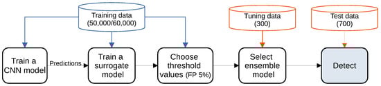
Figure 1.
Pipeline for detecting adversarial examples using surrogate models. A CNN model is trained on the training data (50,000 for CIFAR-10 and 60,000 for MNIST and Fashion-MNIST). Then, a surrogate model is trained on the predictions of the CNN model using features derived from the training data directly (raw image and the Histogram of Oriented Gradients) or through the CNN model (activations). Threshold values for surrogate detectors are chosen on the training data, targeting a desired false positive rate. After that, we select an ensemble model on the tuning set, which consists of generated adversarial examples. Finally, we test our model on the test data. Blue subsets represent unmodified examples, whereas orange represents adversarial examples. All subsets are non-overlapping.
Most of these methods are designed to handle one-dimensional input; to handle a two-dimensional image, preprocessing is needed. To measure the influence of the feature space that surrogates utilise in the detection of adversarial examples, we train surrogates using three different feature spaces: (i) raw images, (ii) the activations of the targeted CNN model (on the last convolutional layer), and (iii) descriptive features extracted from the raw image. Raw images as inputs match the feature space of the surrogates with the CNN model. As preprocessing, the inputs are scaled to the range for the CNN models. The image is further transformed row-wise into a one-dimensional vector. This representation loses the spatial information of an image. Activations as inputs correspond to the representation learned in the fully connected layers of the CNN model. The assumption is that even though the activations are contaminated by the adversarial example, the adversarial example is meant to fool the final classification [31], so the activations might still carry useful features for the detection.
To obtain a one-dimensional activation vector suitable for the surrogate models, we utilise the inputs to the last layer in the CNN. Thus, all layers up to the final (fully connected) layer, e.g., the convolutional and pooling layers, are applied. The resulting activations are standardised to have a zero mean and a variance equal to one. In order to filter “adversarial” features, i.e., features that predominately pick up information relevant to the perturbations, Principal Component Analysis (PCA)—a dimensionality reduction technique—is applied on the activations, and 16, 32, or 64 components are selected. Lastly, extracted features for the surrogate models are obtained using the Histogram of Oriented Gradients (HOG) [41], which uses the distribution of oriented gradients in local neighbourhoods of an image as the descriptor. Hence, while this input space preserves spatial information, it does not match the input space of the CNN model.
Parameters for the Histogram of Oriented Gradients descriptor on the MNIST and Fashion-MNIST datasets are the following: number of orientations is 8, pixels per cell is a tuple (4,4), and cells per block is (1,1), which for an image produces a vector of length 392. On the CIFAR-10, the number of orientations is 9, pixels per cell is a tuple (8,8), and cells per block is (3,3), which for an image produces a vector of length 324. The parameters were chosen by optimising the accuracy of surrogates on the test sets. The parameter values for the number of orientations were 6, 8, and 9, values for pixels per cell (2,2), (4,4), (6,6), and (8,8), and cells per block were (1,1) and (3,3).
As mentioned earlier, a surrogate model approximates the behaviour of a black-box model: in our case, a CNN. Therefore, when given an input, their decisions should be similar or even equal. Based on that expectation, we formulate the following three methods to detect potential adversarial examples.
4.1. Prediction Deviation
This method compares the prediction of a CNN and its surrogate model. Let’s suppose an adversarial example fools the targeted CNN model to a class . The input either fools a surrogate of the CNN model or not, i.e., changes its prediction for that input or does not influence it. If a surrogate model deviates from the CNN, i.e., they predict different classes, then the input is flagged as potentially adversarial. The assumption is that the adversarial example generated for the CNN model will not fool the surrogate model at all, or not to the same (wrong) class as the targeted model. The false positive rate of the proposed detection strategy depends solely on the ability of the surrogate to mimic the CNN model’s reasoning, i.e., the accuracy of the surrogate test set. This method does not have the ability to control the rate of falsely flagged inputs since there is no threshold value for the detection. Consequently, it may falsely flag many unmodified inputs as adversarial.
4.2. Distance Deviation
Distance Deviation is a refinement of Prediction Deviation. It requires the predictions to be only similar, not equal. We compare the class probability vector of a surrogate model to one of the CNN; the exact way we compute the class vectors is given in Appendix B. The difference is measured using the (Minkowski) distance metric. In this paper, the distance metric (also known as a city block or Manhattan distance) is selected. Therefore, the distance between the prediction vectors of a CNN model and its surrogate model is defined as:
where and represent the class probability vectors of the CNN and the surrogate model, respectively. The range of for the metric is from 0 to 2. The maximum value is reached when each prediction vector consists of 1 for different classes and 0 otherwise. An analysis of the results (cf. Section 6) for Prediction Deviation shows that a surrogate model can approximate the prediction of the CNN on the unmodified images, whereas they disagree most of the time on adversarial images. Therefore, it is expected that is close to 0 on unmodified inputs and closer to 2 on adversarial examples—the prediction vectors are similar on the unmodified inputs, but they deviate notably on adversarial examples. Figure 2 supports this by depicting for unmodified and adversarial examples of the SVM surrogate trained on the activations. The peak of for the unmodified inputs is always near 0, and the peak of for the adversarial examples is near 2. Selecting a threshold value that decides to flag an input as adversarial between the two distributions is a balance between a high detection rate and false alarms. Examples that achieve higher than the threshold value are flagged as adversarial. The concrete threshold value is selected on the training set.
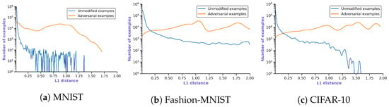
Figure 2.
Histograms of the values (logarithmic scale) for the CNN and their best surrogate (SVM) utilising Distance Deviation trained on the activations of the CNN across three datasets. The blue line represents on the unmodified inputs—a set used for choosing a threshold value—while the orange line represents on the generated adversarial examples.
4.3. Confidence Drop
A CNN classifier outputs a class probability vector that indicates how confident it is in the prediction. The predicted class is the class that has the maximum class probability in the vector. For example, if a CNN network is trained on a dataset that has 10 classes, then the predicted class has a probability of at least 0.1 if all classes are equally likely. The learning algorithm that is used to train the CNN classifier utilises the Cross-Entropy loss function that steers the CNN model towards more confident predictions.
Confidence Drop is thus based on the confidence of the predicted class. Several attacks are able to craft adversarial examples that are classified wrongly with high confidence, e.g., BIM. Therefore, instead of observing the confidence of the CNN, we look for a drop in confidence of its surrogate—we assume that their prediction is less confident on adversarial examples. In order to confidently rely on the prediction of the CNN model, the probability of the predicted class on an input should be above a threshold value. If this idea is extended further to surrogate models, then the prediction of a CNN model should not be trusted if the CNN model or its surrogate model has a value below threshold values, which are selected for each model independently. Figure 3 depicts our assumption by plotting the confidence of the SVM surrogate trained on the activations. An example is flagged as adversarial if the prediction of a surrogate has a confidence lower than a threshold value. This method differs from the aforementioned ones in the way that it is not assumed that a CNN and its surrogate behave similarly.
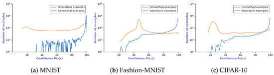
Figure 3.
Histogram of predicted class probabilities of the best surrogate (SVM) utilising Confidence Drop and trained on the activations across three datasets. The blue line represents the unmodified inputs, and orange is the adversarial examples.
The threshold values are determined so that the FP rate on the validation set reaches a certain value n. A threshold value is a confidence that ranks in n-th percentile of the predicted class probabilities in descending order. Therefore, all examples that have predicted class confidence lower than the threshold are considered adversarial. The main idea of the detection strategy is the assumption that the prediction of a CNN model or its surrogate, which approximates the predictions of the CNN model, is less confident with adversarial examples. This strategy differs from the aforementioned strategies, Prediction Deviation and Distance Deviation, in the way that it is not expected that a CNN model and its surrogate behave similarly, i.e., predict the same class or have similar prediction vectors.
To compensate for the potential shortcomings of individual surrogate models, we consider an ensemble thereof. Moreover, we model an ensemble based on voting—an input is considered as an adversarial example if at least n surrogate models in the ensemble mark it as adversarial. The value of n is decided on the training set. The authors in [42] argue that an ensemble of detectors is weak against an adaptive attacker, i.e., an attacker that targets the detection method and the CNN model. However, in Section 6, we show that ensembles enhance the prediction of single models, and in Section 6.4, where we simulate an adaptive attacker in a grey-box setting, our methods achieve results relatively similar or even equal to defence against a normal attack.
5. Evaluation Methodology
This section describes the evaluation methodology, including the utilised benchmark datasets, the attacks considered for generating adversarial examples, and the evaluation metrics. We compare our defence to four state-of-the-art defence methods: namely Feature Squeezing, MagNet, Pixel Defend, and Subset Scanning, all of which are described in Section 2.
5.1. Datasets
The first dataset is the well-known handwritten digit database MNIST [43], which has been extensively studied in the domain of adversarial attacks. The database contains 60,000 training and 10,000 testing images. All images are in greyscale and are sized pixels. All digits are centred and normalised in size.
Fashion-MNIST [44] is modelled analogously to MNIST regarding size, colour tone, and number of classes and is intended as a more challenging replacement to MNIST. The goal is to distinguish types of clothing, such as trousers, pullover, shirt, or trainers.
CIFAR-10 [45] is also often used for demonstrating adversarial examples. It consists of 60,000 colour images of 32 × 32 pixels divided into 50,000 training and 10,000 test images. The 10 classes include airplane, automobile, cat, dog, horse, ship, or truck.
For each dataset, we selected a state-of-the-art CNN according to these main requirements: reasonable computational effort, a network that does not utilise an ensemble, and high performance on the dataset. The models chosen for MNIST, SimpleNet [46], and Fashion-MNIST, DualPath network [47] with WideResNet28-10 [48], denoted as DualPath_28_10, achieve an accuracy similar to state-of-the-art results (https://paperswithcode.com/) (accessed on 16 October 2023). For CIFAR-10, the chosen CNN, DenseNet [49], achieves an accuracy of 94.48%, whereas the best accuracy of 99.70% is achieved by EffNet-L2 [50]. Nevertheless, the results that DenseNet achieves on CIFAR-10 are sufficient to demonstrate our novel detection methods.
Each dataset is split into training (50,000 for CIFAR-10 and 60,000 for MNIST and Fashion-MNIST). We generate 1,000 adversarial examples, split into a subset for selecting detector parameters and model selection (300 images), i.e., the tuning set, and a subset on which the results are tested (700 images).
To prepare the output of a convolutional layer as input for the surrogates, preprocessing is needed. Preprocessing of the SimpleNet activations is carried out by a simple squeezing operation, which is used to remove single-dimensional entries from the shape of a matrix. On the other hand, DualPath_28_10 and DenseNet activations are transformed by Average Pooling.
The hyperparameters for surrogate models are obtained from a grid search: a grid of parameters is defined for each model, and models are trained with every combination of these parameters. After that, the model that achieves the highest accuracy is selected.
5.2. Attacks
We evaluate our methods on the attacks described in Section 2. These are chosen to cover a variety of approaches in generating adversarial examples: simple attacks that utilise gradient information (FGSM), iterative attacks (BIM and DeepFool), attacks constructed as optimisation problems (PGD and Carlini and Wagner), attacks that use Saliency Maps (JSMA), and attacks that create universal perturbation. These universal perturbations are obtained for the aforementioned attacks in 20 passes on the batch, excluding the CW attack, due to the long generation time (about four hours for one pass). Epsilon values used for the gradient attacks (FGSM, BIM, and PGD) are 0.1, 0.2, and 0.3 with a step of 0.01 for BIM and PGD. We used the parameters proposed by the authors for other attacks. The parameters are also listed in Table 2.
Table 2.
Parameter settings for the used attacks. The variable x represents epsilon values: 0.1, 0.2, or 0.3.
In total, we thus test our detection methods against 23 specific attacks (12 individual and 11 universal (Carlini–Wagner is excluded from universal attacks due to infeasible computation time)). Motivated by [18], we generate 1000 images (randomly selected, therefore the classes in the subset are similarly sized) adversarial examples, resulting in a total of 23,000 adversarial images. We utilise the implementations by the Adversarial Robustness Toolbox (ART) [51] except for the CW attack, for which the implementation from advertorch [52] is used due to higher efficiency. To avoid generating easily detectable images, each adversarial example is clipped inside the valid range [0.0, 1.0].
The CW, BIM, and PGD attacks all achieve high success rates: usually at or close to 100%. FGM achieves very varied results depending on the dataset and the attack strength (epsilon); its success ranges between a low 8% for low epsilons on SimpleNet on MNIST to around 90%. JSMA ranges from 70 to 90%. The universal attack using JSMA as the base attack shows intriguing properties. Specifically, the attack adds equal noise to all the pixels, resulting in an adversarial image that is an original image with higher brightness. Detailed results can be seen in Table A1, Table A2 and Table A3. We can also observe that the CW attack generates adversarial images with the smallest perturbation at the cost of longer generation time.
5.3. Evaluation Metrics
Motivated by [21], three types of image inputs are considered in the detection: successful adversarial example (SAE), failed adversarial example (FAE), and unmodified input. An SAE input is an adversarial example that managed to deceive the targeted CNN, while an FAE input is an adversarial example that failed to deceive the CNN. Nevertheless, it is important to flag that input as a potential threat, as it might stem from an early-stage attack.
We measure the detection performance using the detection rate on successful adversarial examples (SAE rate) and on failed adversarial examples (FAE rate) as well as by measuring the false positive rate (FP rate), i.e., unmodified inputs that are flagged as adversarial examples. The goal is to have a detector that has high overall SAE and FAE detection rates but a low FP rate. However, our main focus is on creating a balance between a high SAE and a low FP rate. Therefore, in order to quantify that balance, we introduce a new detection metric as a harmonic mean of both. This metric is inspired by the F-score, which provides a harmonic mean between precision and recall. It exhibits a parameter that controls that balance. In our metric, precision is analogous to an SAE rate, v, and recall to the complement of an FP rate, i.e., we take the complement of the FP rate, and we seek to maximise that complement. Specifically, our metric is defined as:
where is chosen such that the FP rate is considered times more important than the overall SAE detection rate. Selecting a value is application-specific. In our evaluation, is set to 1.5 so that the FP rate is preferred over the SAE rate. This is due to the fact that some surrogate models achieve a high SAE detection rate at the cost of a high FP rate, which we want to prevent. Nevertheless, we present an F1 score value as well, i.e., = 1.0.
6. Evaluation
In this section, we report the results from our evaluation and compare them to state-of-the-art detection methods. As mentioned earlier, the threshold value for the detection methods represents a balance between a high SAE detection rate and a low FP rate, and all threshold values are tuned on the training set. In order to compare our approaches with other state-of-the-art methods, the threshold values are selected so that the detector achieves an FP rate of 5% on the training set, which is a value often used in related work (e.g., [21]). We sort all the detection values on the training set in ascending order and take the value at the fifth percentile for Distance Deviation, and we use descending order and the fifth percentile for Confidence Drop. In an ensemble, first a threshold value for each model is set so that the model achieves an FP rate of 5% as above, and then the number of votes n needed to flag a sample as adversarial is selected so that the FP rate of the ensemble is closest to the targeted FP rate. However, the targeted FP rate is not always 5% on the test set; therefore, we propose the harmonic rate presented in Section 5.3.
6.1. Evaluation Configuration
In the following, we summarise specific parameter settings and configurations used in our evaluation.
Feature space: We trained surrogate models using three feature spaces: raw images, the activations of the CNN, and extracted features (Histogram of Oriented Gradients). Due to the low accuracy achieved by surrogates for CIFAR-10 on raw images and extracted features, we consider only results on the activations as inputs for these. Figure 4 shows the influence of the three input types on the harmonic rate on the Fashion-MNIST dataset; the surrogates follow the same trend on the MNIST dataset. We observed that there is no input space that performs the best for all three detection methods. When utilising Prediction Deviation, the highest harmonic rate is achieved with raw images, followed by extracted features. The surrogates trained on the activations achieve notably lower harmonic rates, except the GNB and the SVM. The influence of the feature space is less evident when surrogates utilise Distance Deviation, except for DT and GNB, which perform notably better on the activations. When the Confidence Drop method is used, activations outperform other input types, which achieve a harmonic rate lower than 50.
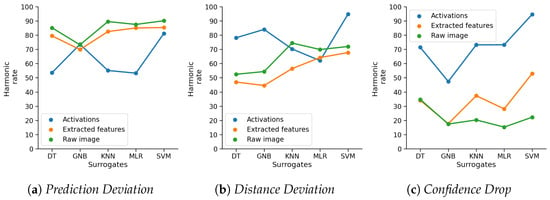
Figure 4.
Influence of feature space on the harmonic rate of the surrogates on Fashion-MNIST.
PCA filtering: The activations of the CNN models were transformed using principal components. The best surrogate model utilising activations as input is the SVM surrogate. We observed that when selecting 64 components, the harmonic rate of the SVM detector always improves (marginally or notably). The harmonic rates of other surrogates decreases in certain settings. However, when utilised with SVM in an ensemble, we manage to improve the harmonic rate of the SVM surrogate as an individual detector. Overall, we suggest transforming the activations of SimpleNet with 16 PCs and activations of DualPath_28_10 and DenseNet with 64 PCs.
Ensembles: An ensemble is constructed from all combinations of surrogate models trained on the same input type; thus, a total of (31) different ensembles are built. The ensemble that achieves the highest harmonic rate on the tuning set is chosen. We provide our observations for the best-performing individual surrogate models. The improvement is least evident on MNIST and is at most 0.11 since the surrogate models already achieve a high harmonic rate (at least 93.15). On Fashion-MNIST and CIFAR-10, the best-performing individual models achieve a lower harmonic rate of at least 89.98 and 80.69, respectively. Therefore, the improvement to the ensembles is higher than on MNIST: namely, up to 2.08 on Fashion-MNIST and 10.50 on CIFAR-10.
Comparison to State-of-the-Art: We compare our methods to the state-of-the-art approaches mentioned in Section 2: Feature Squeezing, MagNet, PixelDefend, and Subset Scanning. All aforementioned detection methods utilise threshold values to decide if an input is considered adversarial or not. We choose a threshold value so that the FP rate of the detectors on the training set is 5%, as motivated by [21]. For a fair comparison, the best-performing parameter settings for state-of-the-art methods are estimated on the tuning set and are tested on the same subsets as the best-performing ensembles. For the state-of-the-art methods, we choose the parameters suggested by the authors. For datasets on which no results were reported, i.e., Feature Squeezing and MagNet on Fashion-MNIST and PixelDefend on MNIST and Fashion-MNIST datasets, we tried to tune the parameters to the best of our knowledge to achieve the highest performance.
6.2. Results of the Basic Defence
In the following, we present and analyse the results of using our three defence methods in the basic setting, i.e., without an adaptive attacker.
6.2.1. MNIST
The best-performing ensemble for SimpleNet and Prediction Deviation achieves a harmonic rate of 95.56, as seen in Table 3. It consists of k-NN and MLR on raw images with , which means that an example is considered adversarial if both detectors mark it as such. The highest harmonic rate of 94.22 for a detector utilising Distance Deviation is achieved by the DT, k-NN, and SVM ensemble on raw images with threshold values of 1.9366, 0.7695, and 0.9345, respectively, and . We note that in general, a lower threshold value is preferred, as that increases the sensitivity of the detector towards adversarial examples. The DT has a very high threshold, meaning that most of the adversarial examples will bypass its detection—however, it might still help in the detection of certain examples when utilised in the ensemble. The best ensemble for Confidence Drop is the DT and SVM ensemble on the first 16 principal components of the activations: achieving a harmonic rate of 93.18 and with threshold values of 100% and 99.94%, respectively, and . The DT overfit to the attack patterns since it has a very high confidence threshold of 100%, but it achieves a low SAE detection rate of 26.77 as an individual detector due to high confidence on adversarial examples, too. However, it slightly enhances the SVM surrogate in an ensemble. As shown in Table 3, all the detectors achieve an FP rate close to the desired value of 5.00 except for Prediction Deviation, which achieves the lowest FP rate of 2.45. Distance Deviation does not work well against the CW attack, achieving an SAE detection rate of 85.82. All proposed methods are vulnerable against FGSM with , against which they achieve SAE detection rates of 72.41, 77.59, and 81.03, respectively. Confidence Drop struggles to detect adversarial examples generated by the BIM and PGD attacks with and , achieving SAE detection rates between 50.34 and 73.38.
Table 3.
Surrogates for SimpleNet on the MNIST dataset together with state-of-the-art approaches; detection rates in % for successful adversarial examples.
From the state-of-the-art methods for SimpleNet, Feature Squeezing achieves high detection rates against all attacks excluding BIM with and , against which it achieves an SAE detection rate of 84.32 and 73.67, respectively. MagNet showed no vulnerability against any of the tested attacks and achieved SAE detection rates of 100.00 against all of them. We observe that PixelDefend is vulnerable to the JSMA attack, against which it achieves an SAE detection rate of at most 88.63, whereas for other attacks it achieves an SAE detection rate of 100.00. Subset Scanning shows similar behaviour as PixelDefend, i.e., it achieves a perfect SAE detection rate of 100.00 against all attacks except JSMA, against which it achieves a 72.95 SAE rate. Only Prediction Deviation and Distance Deviation achieved low FAE detection rates of 6.69 and 42.74, respectively. The highest harmonic rate is achieved by Feature Squeezing at 97.01, whereas our methods, Prediction Deviation, Distance Deviation and Confidence Drop, achieve harmonic rates of 95.56, 94.22, and 93.18, respectively. Prediction Deviation has a similar harmonic rate to PixelDefend and Subset Scan even though it has a much lower SAE detection rate of 91.35 compared to PixelDefend (98.38) and Subset Scan (96.14) due to a low FP rate of 2.45 compared to the FP rates of PixelDefend (5.04) and Subset Scan (4.60).
It is worth mentioning that when using the DualPath_28_10 network as a classifier for MNIST, our detection strategies achieve better performance, as shown in Table 4. They might thus be better suited as detectors for this type of network, and maybe SimpleNet for MNIST is a combination that does not exhibit sufficient differences between the fully connected layer of the CNN compared to the shallow classifiers we employ.
Table 4.
Surrogates for DualPath_28_10 on the MNIST dataset together with state-of-the-art approaches; detection rates in % for successful adversarial examples. Universal and FGSM attacks are averaged.
The best-performing surrogate ensembles of DualPath_28_10 for each proposed detection strategy are the k-NN surrogate on raw images utilising Prediction Deviation, with a 97.21 harmonic detection rate; the DT and SVM weighted ensemble with and thresholds 0.043 and 0.042, respectively, trained on the activations processed with 64 principal components utilising Distance Deviation, with a 96.01 harmonic detection rate; and the DT, k-NN, and SVM weighted ensemble with and thresholds 100.00%, 100.00%, and 99.68%, respectively, trained on the activations processed with the first 64 principal components utilising Confidence Drop and achieving a 96.87 harmonic detection rate.
We further tried to combine two of our methods, namely, Confidence Drop and Prediction Deviation, on the primary architecture used for this dataset, i.e., SimpleNet. We used an ensemble of k-NN and MLR with for Prediction Deviation and for Confidence Drop with confidence thresholds of 52.46% and 47.41%. The performance increased for the attacks against which Confidence Drop struggled when used as a single predictor—namely, all but one variant of the BIM, all variants of PGD, universal BIM, and one variant of universal PGD—while only marginally worsening in the other settings. Thus, it achieves an overall slightly higher harmonic rate, showing that these two methods can be combined together to achieve an overall more reliable detector, and both methods can be recommended as detectors.
6.2.2. Fashion MNIST
On Fashion-MNIST, the target model is DualPath_28_10. The best-performing ensemble utilising Prediction Deviation is made of k-NN and SVM with on raw images, which achieves a 92.03 harmonic rate. The GNB and SVM ensemble on the first 64 principal components of the CNN achieves the highest harmonic rate of 95.42 among ensembles that utilise Distance Deviation. The ensemble parameters are , and distance thresholds are 0.3918 for GNB and 0.3762 for SVM. Note that these threshold values are much lower than the thresholds of the best-performing ensemble on MNIST. The best ensemble that utilises Confidence Drop uses the same input type, i.e., the first 64 principal components of the CNN activations, and consists of MLR and SVM with and confidence thresholds of 71.87% and 81.56%. This ensemble achieves a 95.49 harmonic rate.
Most of the detectors achieve an FP rate higher than 5.00 except Feature Squeezing (4.45) and Subset Scan (4.90). MagNet achieves the highest FP rate of 7.27, as shown in Table 5. In contrast to their performance on MNIST, Distance Deviation and Confidence Drop achieve higher harmonic rates of 95.42 and 95.49, respectively, compared to Prediction Deviation at 92.03. PixelDefend, Distance Deviation and Confidence Drop achieve a perfect detection rate of 100.00 against first-order attacks, i.e., FGSM, BIM, and PGD. Moreover, Distance Deviation and Confidence Drop achieve a 100.00 SAE detection rate against the Universal JSMA attack, which fools other approaches notably. Feature Squeezer achieves an SAE detection rate between 65.51 and 77.27 against FGSM attacks. CW, DeepFool, and JSMA and its universal version avoided most of the detection of PixelDefend, against which it achieves SAE detection rates of 11.13, 20.46, 26.26, and 49.76, respectively. Subset Scanning achieves a very low SAE detection rate against JSMA (13.65) and its universal version (15.31).
Table 5.
Surrogates and state-of-the-art approaches for DualPath_28_10 on the Fashion-MNIST dataset; detection rates in % for successful adversarial examples. Universal attacks excluding Universal are averaged.
Again, we combined Prediction Deviation and Confidence Drop using an ensemble of MLR and SVM with thresholds of 71.87% and 81.56%. For a small increase in the FP rate compared to Confidence Drop, the detection improved against almost all attacks except the average against universal attacks, where it, however, decreases by a mere 0.06%, at a very high rate of 99.81%. Thus, we can recommend the combination of the methods above over the single Confidence Drop approach.
6.2.3. CIFAR-10
As mentioned before, results of surrogates for this dataset are reported only on the activations of the CNN model, resp. the first 64 principal components thereof. The best-performing ensembles are the k-NN and SVM ensemble utilising Prediction Deviation with , achieving an 88.54 harmonic rate; the MLR and SVM ensemble utilising Distance Deviation with and distance thresholds of 0.3934 and 1.0301, respectively, achieving a 92.09 harmonic rate; and the MLR and SVM ensemble utilising Confidence Drop with and confidence threshold of 74.76% and 51.84%, respectively, achieving a 89.24 harmonic rate.
As shown in Table 6, notably higher FP rates than 5.00 are caused by Distance Deviation (5.93), Confidence Drop (7.29), and MagNet (7.29). Distance Deviation and Confidence Drop showed vulnerability against CW, DeepFool, and JSMA attacks, achieving SAE detection rates between 53.05 and 82.83, but they achieved an SAE rate of at least 99.82 against first-order attacks (FGSM, BIM, and PGD) and an SAE rate of 99.63 against universal attacks, excluding Universal JSMA. Moreover, Prediction Deviation showed higher SAE detection rates against CW, DeepFool, and JSMA attacks (between 83.04 and 91.34) but lower SAE rates against first-order attacks (at most, 85.26). Feature Squeezer achieves high detection rates against CW (96.05) and DeepFool (93.86) attacks. However, it does not perform well against the first-order and universal attacks (However, it has to be noted that on this dataset, we did not manage to reproduce the results reported by [21], albeit utilising the same settings and target model as they reported. The discrepancy in the results might come from the difference in the generation process of the adversarial examples. We crafted examples on a CNN model with the logits as the last layer, which is recommended by the authors of the adversarial library, whereas the authors in [21] used a model with the softmax layer as the last one. The authors state better results on first-order attacks, with an average SAE rate of 83.6, on a slightly less diverse set of attacks than tested by us. This result is, in any case, still lower than our best result).
Table 6.
Surrogates for DenseNet on the CIFAR-10 dataset together with the state-of-the-art approaches; detection rates in % for successful adversarial examples. Universal attacks excluding Universal JSMA are averaged.
MagNet achieves low SAE rates against the FGSM attack (at most 53.79) but very high SAE rates against its iterative versions (at least 99.39). Furthermore, MagNet achieves lower detection rates against universal attacks in comparison to Distance Deviation and Prediction Deviation. Similarly to Distance Deviation and Prediction Deviation, PixelDefend and Subset Scan show vulnerability against CW, DeepFool, and JSMA attacks, but they achieve much lower SAE detection rates of at most 6.69, 6.43, and 8.36, respectively. However, Subset Scan shows very high SAE rates against the first-order attacks (at least 99.70) and universal attacks (98.84), excluding Universal JSMA, against which all detection methods achieve a low rate.
Again, we further tried to combine two of our methods: namely, Confidence Drop and Prediction Deviation. We used an ensemble of MLR and SVM with for Prediction Deviation and for Confidence Drop with confidence thresholds of 59.40% and 37.99% and ; we aimed for a lower FP rate of the ensemble utilising Confidence Drop to keep the overall FP rate within the targeted 5%. The performance increased against CW, DeepFool, and JSMA, against which Confidence Drop struggled. Achieving a harmonic rate of 94.65, we showed that these two strategies can be combined together and complement each other also on this dataset.
6.3. Changing the Tuning Set
We utilised the tuning set to select an ensemble model that would potentially perform the best in the test phase. Moreover, the parameters for the state-of-the-art methods against which we compare our results were selected on the same set. So far, the tuning set used in our evaluation consisted of adversarial examples generated by all attacks—therefore, we implicitly assumed that the attacks would be known in the test phase. This thus provides an upper bound of achievable defence if the defender has extensive information on the attack strategy. Therefore, we evaluated both our defence as well as the state-of-the-art defences on tuning sets that consist only of adversarial examples generated by one of the available attacks in order to test how well these transfer to other attacks. In that way, we estimate how general the methods are when the defender has little to no knowledge about the attacks. To provide a lower bound on the success rate, we also tried a default setting where we assume no prior knowledge of adversarial attacks—there is no tuning set on which we select an ensemble. In that setting, we select an SVM surrogate as a single detector. Having the same results for different tuning sets means that the same detector is selected for both. We do not test PixelDefend on different tuning sets since it does not utilise a tuning set to select its parameters.
On the MNIST dataset in Figure 5, detectors that utilise Prediction Deviation and Distance Deviation achieve similar results in terms of harmonic rate despite different tuning sets used, whereas detectors that utilise Confidence Drop have more volatile performance. Ensembles that utilise Distance Deviation achieve a high FP rate of 9.21 when either CW or FGSM attacks are used in tuning sets. Confidence Drop ensemble models chosen on either CW, JSMA, DeepFool, or FGSM attacks achieve low detection rates against the BIM and PGD attacks. However, they achieve harmonic rates of at least 84.67 due to low FP rates that compensate for low SAE detection rates. Feature Squeezer, MagNet, and Subset Scan have the same results for most of the variations of tuning sets except for the tuning set based on BIM for Feature Squeezer and JSMA for Subset Scan.
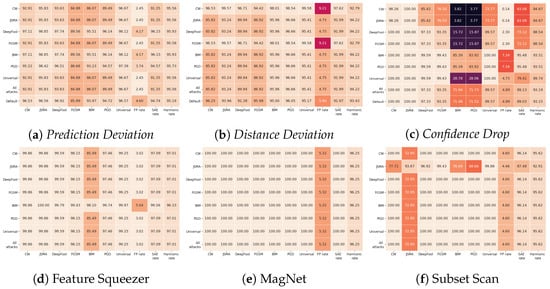
Figure 5.
Tuning set transferability on MNIST; detection rates in % for successful adversarial examples.
The impact of the tuning set on Fashion-MNIST shown in Figure 6 is less obvious in the proposed detection methods compared to state-of-the-art methods. The biggest difference for ensembles utilising Distance Deviation is on tuning sets consisting of either CW or JSMA, and for ensembles utilising Confidence Drop, it is on tuning sets consisting of CW and DeepFool. Feature Squeezer has the biggest difference in results for detectors chosen on either CW or DeepFool, achieving harmonic rates of only 38.80 and 54.44, respectively, in comparison to the highest result of 82.13. MagNet and Subset Scan do not have those big oscillations in harmonic rates, but the performance of the detector on certain attacks depends widely on the tuning set. For example, MagNet achieves a detection rate against BIM of 100.00 or 0.00 depending on a tuning set consisting of BIM or DeepFool, respectively.
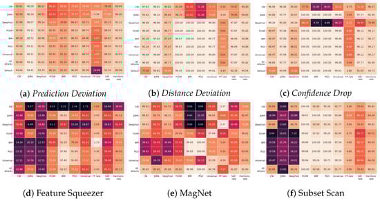
Figure 6.
Tuning set transferability on Fashion-MNIST; detection rates in % for successful adversarial examples.
All tested methods (proposed and state-of-the-art) are volatile to the selection of a tuning set on the CIFAR-10 dataset, as shown in Figure 7. Prediction Deviation achieves the least variance in the harmonic rate, whereas Feature Squeezer has the most, varying from 5.10 to 66.68. All proposed methods, Prediction Deviation, Distance Deviation, and Confidence Drop, struggled to detect BIM and PGD when a tuning set consists of either CW, JSMA, DeepFool, or FGSM attacks. Similar behaviour can be seen for MagNet. Feature Squeezer manages to detect CW, JSMA, and DeepFool only when a tuning set consists of one of those attacks. In contrast to others, Subset Scan shows the most stable harmonic rates across different tuning sets—excluding the tuning sets consisting of either CW or DeepFool attacks, where it achieves harmonic rates of 13.64 and 50.84, respectively.
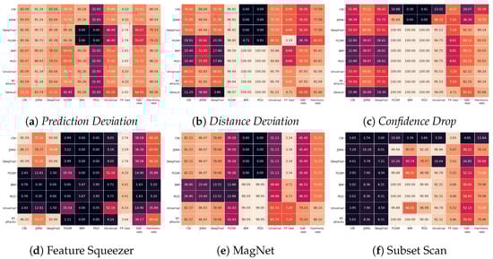
Figure 7.
Tuning Set transferability on CIFAR-10; detection rates in % for successful adversarial examples.
From the evaluation with a variable tuning set, we observe that the default setting utilising one of the proposed methods showed similar results to those of ensembles chosen on the tuning set consisting of all attacks on the MNIST and Fashion-MNIST datasets, whereas on the CIFAR-10 dataset, the difference in the harmonic rate is most evident for Confidence Drop: from 89.24 with all attacks in the tuning set to 83.66 for the default setting. Moreover, ensembles chosen on the tuning set consisting of only CW attacks showed the worst performance for all proposed methods across three datasets. If only one attack is available for generating a tuning set, we recommend either BIM or PGD since the ensembles chosen on those tuning sets achieve harmonic rates that are the closest to the best ones. Ensembles chosen on Universal attacks showed better performance than ensembles chosen on either BIM or PGD attacks in some settings, but the tuning set consisting of Universal attacks uses all other attacks, e.g., Universal FGSM, Universal DeepFool, etc.
6.4. Adaptive Attacker
To get a better understanding of how our detection methods might perform against adaptive attacks, we perform an adaptive attack specifically created to target a given detection method after the method has been completely specified. The authors in [53] argued the importance of testing detection methods against adaptive attacks to get an approximation of how strong the detection method is in a real-world setting.
As defined in Section 3, the adaptive attack carried out in this paper follows a threat model wherein we assume the attacker has white-box knowledge of the CNN (the target/victim model) and grey-box access to the surrogate models. In other words, the attacker is aware of the surrogate models used in an ensemble and their hyperparameters but does not have access to either their parameters nor to the original dataset that the surrogates were trained on. Instead, the attacker has to obtain a similar dataset and train the surrogate models on them. Consequently, those models will have different weights and different threshold values compared to the original ones. We consider this as a realistic scenario since on the one hand, the CNN architecture and its learned parameters might be publicly available (or can be obtained or approximated, e.g., via a model extraction attack [54] if the model is exposed for querying access, e.g., via an API), but on the other hand, the learned parameters of the detection method are not published and cannot be queried.
The authors in [42] argue that ensembles of detectors are weak against an adaptive attacker. However, they consider that an attacker has white-box access to the detection method as well, whereas we consider a scenario wherein details about the detection used are partially known (grey-box access), and the CNN’s architecture and its learned parameters are publicly available.
We considered the EMNIST Balanced [39] and STL-10 datasets [40] as (surrogate) datasets that are similar to the MNIST and CIFAR-10 datasets, respectively. We are not aware of a fitting dataset for the Fashion-MNIST. The attacker uses these datasets to train his/her own detector with weights as close as possible to those of the original detector used by the defender.
As some of the surrogate models used in the ensembles are non-differentiable, e.g., DT, GNB, and k-NNN, we decided to use a score-based attack that utilises Particle Swarm Optimisation (PSO), as in [55]. The authors claim that the attack uses a low number of queries to generate adversarial examples with high success rates. The attack is black-box since it only queries the targeted model and observes the labels it returns without any other knowledge about the model. The loss function that the PSO algorithm optimises tries to reduce the confidence of the true class on the adversarial input:
so that it maximises the difference between the confidence of the true class on the unmodified and adversarial input . We call the original loss function . The algorithm stops when an adversarial image manages to deceive the targeted CNN model. The perturbations are controlled by defining an upper bound distance between the unmodified image and the adversarial image.
The goal of our adaptive attack is to fool the targeted CNN model and bypass detection at the same time. We incorporated a detection term in the loss function that the PSO attack optimises:
where n is the number of surrogates in the ensemble. The constant c is chosen so that the and the are on the same scale. The detection term is created specifically for each method. For Distance Deviation, we optimise so that the distance between the prediction vectors of the targeted CNN and a surrogate model is smaller than the threshold value. Therefore, , where we sum distances of the targeted CNN model and each surrogate model in the ensemble. The c constant is set to 2, as the distance has a range between 0 and 2, whereas the confidence has a range between 0 and 1. We used the same for Prediction Deviation since detection is bypassed when the targeted CNN and a surrogate model predict the same label, which implies that their prediction vectors are similar. In order to fool Confidence Drop, the attacker should craft an adversarial example so that the confidence of the predicted class of a surrogate model is higher than the threshold value; therefore, .
The PSO stops when the adversarial example fools the targeted CNN model and bypasses detection. The parameters are set as proposed by [55]. We evaluated the adaptive attack on the first 100 samples in the test set that were not already successful adaptive attacks, i.e., on images that were correctly classified by the CNN model and not flagged as adversarial. We also present the statistics for the PSO attack on the targeted CNN without defence as a benchmark.
We are aware that a gradient-based attack could be used against non-differentiable models with some modifications, as in [56]. However, we chose the PSO attack as a strong attack that achieves a 100% success rate against the targeted CNN model without a defence, i.e., it generates a successful adversarial example against the targeted CNN model for every sample in the subset.
We performed the experiment in a way that the adversarial examples are crafted to deceive the original CNN model and the surrogate models trained on a similar dataset. The results are then reported using the original CNN and the original surrogate models as detectors.
As shown in Table 7 and Table 8, the number of queries and iterations needed for the adaptive attack is much higher compared to a regular attack on the CNN model. For example, on the MNIST dataset, the regular attack has on average 4.98 iterations, while the adaptive attack for Confidence Drop takes 761.47 iterations, i.e., a 152-fold increase.
Table 7.
Adaptive attack on MNIST; detection rates in % for successful adversarial examples.
Table 8.
Adaptive attack on CIFAR-10; detection rates in % for successful adversarial examples.
The detection rates of Prediction Deviation, Distance Deviation, and Confidence Drop on MNIST are 74.26%, 16.83%, and 89.11%, respectively. For reference, their average detection rate against the attacks on the CNN model without a defence on the MNIST dataset in Section 6 is 90.82%. A similar trend is observed on the CIFAR-10 dataset, for which the best performing model is Confidence Drop, with a 72.27% detection rate; after it, Prediction Deviation has a 69.30 % rate, and the worst-performing Distance Deviation has a 51.48% rate. Their average detection rate in Section 6 is 81.92%.
An explanation for the low detection rate of Distance Deviation is that the threshold that surrogates use is relatively high, i.e., an average threshold is 0.85 on MNIST and 0.71 on CIFAR-10. The distance is in the range from 0 to 2, and threshold values closer to 0 are favourable. Due to the high threshold value, the attacking space is larger compared to that of Prediction Deviation. Consequently, the prediction vectors of the CNN model and its surrogate can be similar enough, i.e., their distance is lower than the threshold value, even if they predict different classes. For example, if Prediction Deviation is used on the images crafted against Distance Deviation, the detection rate jumps from 16.83% to 80.19% on the MNIST dataset and from 51.48% to 78.22% on CIFAR-10 (This is an example of the superiority of Prediction Deviation over Distance Deviation in this setting. Detection rates are higher than those reported in Table 7 and Table 8 because here we do not stick with our initial assumption that adversarial examples are crafted specifically to fool the targeted detection method. In other words, the attacker could proceed with the crafting of an adversarial example until it potentially fools Prediction Deviation as well). The best-performing method against the adaptive attacker is Confidence Drop, which on the MNIST dataset has no degradation in detection rate, i.e., in Section 6, it achieves a rate of 89.12%, and in Table 7 it achieves a rate of 89.11%. This stems from the fact that it is hard to craft an adversarial example that will fool the CNN model and at the same time achieve high prediction confidence on all of its surrogates, i.e., one of the surrogates usually has low confidence in the adaptive example and thus successfully detects it. For example, the average threshold confidence of the surrogates on MNIST is 99.97%, whereas the average confidence of the least confident surrogate on adaptive examples is 40.96%; on CIFAR-10, the average threshold is 63.30%, and the average confidence of the least confident surrogate on adaptive examples is 48.46%.
7. Discussion and Future Work
We presented three methods based on surrogate models to detect adversarial examples and evaluated these against seven different techniques to generate adversarial examples. The results show that the surrogate models can be used to achieve high harmonic detection rates on the tested datasets (MNIST, Fashion-MNIST, and CIFAR-10). Combining individual models in ensembles in some settings further increases our detection rates.
Our detection rates are on par and sometimes exceed the state-of-the-art methods PixelCNN, MagNet, Subset Scan, and Feature Squeezer. From our observations and the literature, there is no silver-bullet method that fits all settings and attacks. Thus, the availability of diverse defence methods is important. One advantage of our method is that it rarely fails completely against a specific attack, while some of the other state-of-the-art methods achieve success rates well below 50% or even 30% for several cases. Our method is thus well-generalising to different attacks. Since the ensembles are chosen on a tuning set, we also evaluate with different tuning sets without knowledge of the attack, where our methods show a satisfying level of transferability of parameters chosen on a different type of attack. For the state-of-the-art defences evaluated, similar parameter selection is performed on the tuning set. While transfer success rates differ depending on the datasets, our method is able to outperform the state-of-the-art approaches in several cases, and overall, the state-of-the-art techniques are comparable to our proposed methods. We base our detection method on the principle that a CNN model and its surrogate model should have the same or very similar reasoning given the same input. Therefore, the proposed method is not restricted to image datasets only.
In order to tackle the complexity of a dataset, we relied on the CNN activations as inputs to surrogate models; thus, the surrogate models, even though they are lightweight models, are not expected to completely fail in other scenarios.
We can observe that our methods have varying strengths compared to the state-of-the-art, depending on the model type. As such, when detecting adversarial examples for DualPath_28_10, our method matches or often outperforms the ones from the literature, while for the more-shallow SimpleNet architecture, our method matches or is sometimes marginally worse than the state-of-the-art methods. On the CIFAR-10 dataset, the proposed strategies achieve higher detection rates than PixelCNN, Subset Scan, and Feature Squeezer on the DenseNet architecture. Future work will thus investigate this influence of the model type in greater detail. It might be a general hypothesis that the proposed detection method works better for deeper architectures, but this will need to be confirmed by future work. Overall, we recommend using either the combination detector originating from joining Prediction Deviation and Confidence Drop or using Confidence Drop alone—both methods are overall very reliable and never completely fail.
Finally, we evaluated an adaptive attack, i.e., an attack where the attacker anticipates the defence method. The adaptive attack we carried out in this paper follows a threat model wherein we assume the attacker has white-box knowledge of the CNN and grey-box knowledge of the defence, i.e., the attacker knows the type of defence and its parameters but does not have the exact same training data available as the original model creator. We can observe that compared to the original attack without a defence, now (i) the attack requires a larger amount of queries (and thus processing time) to generate the adversarial examples, (ii) the generated adversarial examples are often more different from the original images than before (as noted also, e.g., in [20]), and (iii) the detection rates of our methods do not drop significantly. Generally, Confidence Drop works the best, especially against the attack on MNIST, where it achieved the same performance as against the original attack without a defence.
Being able to fully assess the effectiveness of a defence, one needs to also put the types of mistakes the method can make, i.e., false positives and false negatives, in perspective. False positives might e.g., deny legitimate users from accessing resources they should be entitled to, which might be an inconvenience; not detecting an attack and allowing unauthorised access likely has a much larger impact. However, these ramifications are also very use-case specific and cannot be answered universally.
Future work will include considering internal layer activations and learning null density models from these, as performed, e.g., in [57] as additional information besides, e.g., Confidence Drop.
Author Contributions
Conceptualization, B.F., R.M. and A.R.; methodology, B.F. and R.M.; software, B.F.; validation, B.F., R.M. and A.R.; formal analysis, B.F.; investigation, B.F.; writing—original draft preparation, B.F. and R.M.; writing—review and editing, B.F., R.M. and A.R.; visualization, B.F.; and funding acquisition, R.M. All authors have read and agreed to the published version of the manuscript.
Funding
SBA Research (SBA-K1) is a COMET Center within the COMET—Competence Centers for Excellent Technologies Programme and is funded by BMK, BMAW, and the federal state of Vienna. COMET is managed by the Austrian Research Promotion Agency (FFG).
Data Availability Statement
Publicly available datasets were analyzed in this paper, namely MNIST (available at http://yann.lecun.com/exdb/mnist/, accessed on 16 October 2023), FashionMNIST (https://github.com/zalandoresearch/fashion-mnist, accessed on 16 October 2023), and CIFAR-10 (https://www.cs.toronto.edu/~kriz/cifar.html, accessed on 16 October 2023).
Conflicts of Interest
The authors declare no conflict of interest.
Appendix A. ROC Curves for Detector
The results provided throughout this paper are focused on a single performance point at a desired false positive (FP) rate that is chosen according to the literature. However, every detector actually has a receiver operating characteristic (ROC) curve. The ROC curve is a graphical plot that illustrates the diagnostic ability of a binary classifier as its discrimination threshold (here, the detection threshold) is varied. The ROC curve is created by plotting the true positive (TP) rate against the false positive (FP) rate at various threshold settings. As it would be infeasible to plot all ROC curves, we exemplify the behaviour. As can be seen in Figure A1a against DeepFool, after a small TP rate at the beginning, the detector achieves a TP rate close to 1 after a certain FP rate; this behaviour is very similar against all attacks—another example is provided in Figure A1b against the JSMA attack.
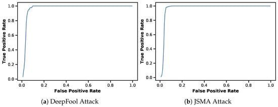
Figure A1.
ROC curve on MNIST against two attacks for the ensemble presented in Table 3.
Appendix B. Class Vector for Surrogate ML Models
In Distance Deviation and Confidence Drop, we utilised prediction vectors of the surrogate models even though not all models use class probabilities for classification. In other words, MLR and GNB output class probabilities by definition, whereas for other models, we used well-accepted techniques for approximating a class probability vector. The class probability vector of DT is estimated as the fraction of samples of the same class as the leaf used for prediction. Likewise, k-NN models its class probability in a similar way, i.e., as the fraction of samples of the same class in the neighbourhood. For all surrogates, we used the implementation in the machine learning package Scikit-learn (https://scikit-learn.org/stable/ (accessed on 16 October 2023)). Specifically, for SVM, we used an implementation in the same package based on [58], where probabilities are calibrated using a pair-wise coupling method. The number of neighbours for k-NN and minimal number of samples in a leaf for DT is higher or equal to the number of classes (for all datasets used, there are 10 classes); therefore, the prediction vector has meaningful class probabilities.
Appendix C. Accuracy of the Surrogates
Surrogates trained on the activations achieve the highest accuracy in approximating the behaviour of the CNN models, as seen in Figure A2. As shown in Section 6, some surrogates that are trained on the activations overfit the specific attack pattern. It is an interesting observation that surrogates that achieve the highest accuracy do not necessarily achieve the highest harmonic rate. For example, the SVM surrogate trained on the activations does not achieve the highest accuracy; however, when utilised for detection, it usually outperforms others. Surrogates using extracted features on the CIFAR-10 dataset achieve very low accuracy; therefore, they are not utilised in our detection methods.
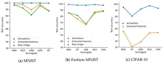
Figure A2.
Accuracy of the surrogates on different input spaces.
Appendix D. Detailed Results and Generation Properties for the Adversarial Example Attacks
Table A1.
Attacks together with their success rate, average distortion , and time needed to generate adversarial examples for the MNIST subset.
Table A1.
Attacks together with their success rate, average distortion , and time needed to generate adversarial examples for the MNIST subset.
| Attack | SimpleNet | DualPath_28_10 | ||||
|---|---|---|---|---|---|---|
| Success Rate | Time | Success Rate | Time | |||
| CW | 100.00 | 0.12 | 9 h 1 m 46 s 745 ms | 99.80 | 0.11 | 21 h 40 m 33 s 646 ms |
| DeepFool | 75.05 | 0.34 | 4 m 2 s 624 ms | 88.11 | 0.32 | 20 m 2 s 628 ms |
| JSMA | 100.00 | 0.42 | 8 m 4 s 367 ms | 98.78 | 0.35 | 13 m 59 s 470 ms |
| FGM-0.1 | 8.85 | 0.24 | 667 ms | 38.41 | 0.24 | 2 s 858 ms |
| FGM-0.2 | 40.44 | 0.49 | 660 ms | 85.67 | 0.49 | 2 s 857 ms |
| FGM-0.3 | 65.09 | 0.72 | 656 ms | 92.78 | 0.72 | 2 s 884 ms |
| BIM-0.1 | 86.12 | 0.22 | 34 s 14 ms | 90.35 | 0.24 | 2 m 34 s 926 ms |
| BIM-0.2 | 100.00 | 0.32 | 33 s 732 ms | 100.00 | 0.44 | 2 m 34 s 934 ms |
| BIM-0.3 | 100.00 | 0.38 | 33 s 702 ms | 100.00 | 0.62 | 2 m 35 s 209 ms |
| PGD-0.1 | 86.12 | 0.22 | 14 m 13 s 133 ms | 91.57 | 0.24 | 1 h 40 m 3 s 368 ms |
| PGD-0.2 | 100.00 | 0.34 | 14 m 12 s 238 ms | 100.00 | 0.46 | 1 h 40 m 14 s 924 ms |
| PGD-0.3 | 100.00 | 0.45 | 14 m 11 s 475 ms | 100.00 | 0.69 | 1 h 40 m 44 s 688 ms |
| UnivJSMA | 44.27 | 0.63 | 20 m 54 s 170 ms | 17.58 | 0.63 | 1 h 2 m 9 s 791 ms |
| UnivDeepFool | 15.59 | 0.42 | 9 m 41 s 462 ms | 52.54 | 0.37 | 1 h 13 m 12 s 857 ms |
| UnivFGM-eps0.1 | 28.67 | 0.45 | 28 s 714 ms | 86.18 | 0.46 | 2 s 567 ms |
| UnivFGM-eps0.2 | 26.06 | 0.48 | 25 s 451 ms | 68.50 | 0.48 | 12 s 537 ms |
| UnivFGM-eps0.3 | 31.59 | 0.50 | 25 s 343 ms | 71.65 | 0.50 | 3 s 109 ms |
| UnivBIM-eps0.1 | 12.07 | 0.32 | 8 m 45 s 813 ms | 82.42 | 0.42 | 28 s 11 ms |
| UnivBIM-eps0.2 | 21.13 | 0.34 | 6 m 37 s 298 ms | 79.17 | 0.47 | 27 s 211 ms |
| UnivBIM-eps0.3 | 14.49 | 0.34 | 6 m 36 s 942 ms | 71.34 | 0.49 | 21 s 988 ms |
| UnivPGD-eps0.1 | 23.04 | 0.36 | 2 h 37 m 29 s 769 ms | 77.54 | 0.44 | 8 m 3 s 688 ms |
| UnivPGD-eps0.2 | 28.87 | 0.37 | 2 h 5 m 27 s 528 ms | 74.29 | 0.48 | 14 m 47 s 863 ms |
| UnivPGD-eps0.3 | 13.68 | 0.44 | 2 h 2 m 1 s 564 ms | 77.54 | 0.50 | 8 m 5 s 145 ms |
Table A2.
Attacks together with their success rate, average distortion , and time needed to generate adversarial examples for the Fashion-MNIST subset.
Table A2.
Attacks together with their success rate, average distortion , and time needed to generate adversarial examples for the Fashion-MNIST subset.
| Attack | SimpleNet | DualPath_28_10 | ||||
|---|---|---|---|---|---|---|
| Success Rate | Time | Success Rate | Time | |||
| CW | 100.00 | 0.03 | 5 h 29 m 38 s 800 ms | 99.79 | 0.01 | 40 h 45 m 51 s 955 ms |
| DeepFool | 69.01 | 0.06 | 3 m 49 s 894 ms | 59.19 | 0.03 | 19 m 53 s 693 ms |
| JSMA | 71.78 | 0.12 | 1 m 33 s 760 ms | 100.00 | 0.10 | 9 m 29 s 483 ms |
| FGM-0.1 | 73.06 | 0.22 | 629 ms | 88.58 | 0.22 | 2 s 943 ms |
| FGM-0.2 | 90.84 | 0.42 | 627 ms | 90.03 | 0.42 | 2 s 833 ms |
| FGM-0.3 | 93.29 | 0.62 | 627 ms | 91.07 | 0.62 | 2 s 847 ms |
| BIM-0.1 | 100.00 | 0.17 | 32 s 29 ms | 100.00 | 0.17 | 2 m 33 s 979 ms |
| BIM-0.2 | 100.00 | 0.27 | 31 s 937 ms | 100.00 | 0.28 | 2 m 34 s 432 ms |
| BIM-0.3 | 100.00 | 0.32 | 31 s 912 ms | 100.00 | 0.35 | 2 m 34 s 452 ms |
| PGD-0.1 | 100.00 | 0.18 | 12 m 39 s 933 ms | 100.00 | 0.17 | 1 h 47 m 5 s 865 ms |
| PGD-0.2 | 100.00 | 0.31 | 12 m 40 s 462 ms | 100.00 | 0.30 | 1 h 46 m 57 s 358 ms |
| PGD-0.3 | 100.00 | 0.42 | 12 m 38 s 518 ms | 100.00 | 0.41 | 1 h 47 m 6 s 843 ms |
| UnivJSMA | 27.90 | 0.51 | 26 m 27 s 324 ms | 32.09 | 0.51 | 44 m 21 s 34 ms |
| UnivDeepFool | 25.13 | 0.19 | 10 m 2 s 932 ms | 56.28 | 0.11 | 1 h 4 m 25 s 954 ms |
| UnivFGM-eps0.1 | 49.73 | 0.34 | 18 s 255 ms | 84.74 | 0.34 | 8 s 965 ms |
| UnivFGM-eps0.2 | 41.11 | 0.37 | 17 s 633 ms | 82.24 | 0.38 | 8 s 799 ms |
| UnivFGM-eps0.3 | 57.72 | 0.37 | 18 s 262 ms | 81.83 | 0.40 | 9 s 342 ms |
| UnivBIM-eps0.1 | 81.15 | 0.32 | 1 m 28 s 174 ms | 86.71 | 0.29 | 18 s 55 ms |
| UnivBIM-eps0.2 | 81.58 | 0.33 | 2 m 48 s 347 ms | 82.35 | 0.30 | 19 s 865 ms |
| UnivBIM-eps0.3 | 71.03 | 0.34 | 39 s 529 ms | 87.12 | 0.31 | 18 s 172 ms |
| UnivPGD-eps0.1 | 79.98 | 0.30 | 1 h 12 m 20 s 30 ms | 85.36 | 0.29 | 16 m 28 s 73 ms |
| UnivPGD-eps0.2 | 84.98 | 0.29 | 1 h 20 m 53 s 146 ms | 83.70 | 0.32 | 5 m 46 s 353 ms |
| UnivPGD-eps0.3 | 82.75 | 0.33 | 1 h 26 m 10 s 425 ms | 83.49 | 0.37 | 5 m 30 s 18 ms |
Table A3.
Attacks together with their success rate, average distortion , and time needed to generate adversarial examples for the CIFAR-10 subset.
Table A3.
Attacks together with their success rate, average distortion , and time needed to generate adversarial examples for the CIFAR-10 subset.
| Attack | DenseNet | ||
|---|---|---|---|
| Success Rate | Time | ||
| CW | 100.00 | 0.00 | 8 h 38 m 31 s 252 ms |
| DeepFool | 52.55 | 0.00 | 18 m 49 s 226 ms |
| JSMA | 100.00 | 0.03 | 5 m 47 s 191 ms |
| FGM-0.1 | 87.13 | 0.20 | 2 s 920 ms |
| FGM-0.2 | 88.40 | 0.38 | 2 s 928 ms |
| FGM-0.3 | 89.79 | 0.56 | 2 s 960 ms |
| BIM-0.1 | 100.00 | 0.12 | 2 m 33 s 926 ms |
| BIM-0.2 | 100.00 | 0.16 | 2 m 33 s 356 ms |
| BIM-0.3 | 100.00 | 0.17 | 2 m 34 s 687 ms |
| PGD-0.1 | 100.00 | 0.13 | 51 m 9 s 740 ms |
| PGD-0.2 | 100.00 | 0.23 | 51 m 22 s 294 ms |
| PGD-0.3 | 100.00 | 0.32 | 51 m 17 s 39 ms |
| UnivJSMA | 11.70 | 0.34 | 24 m 6 s 587 ms |
| UnivDeepFool | 65.43 | 0.04 | 26 m 59 s 453 ms |
| UnivFGM-eps0.1 | 86.49 | 0.26 | 3 s 443 ms |
| UnivFGM-eps0.2 | 87.02 | 0.32 | 3 s 439 ms |
| UnivFGM-eps0.3 | 87.45 | 0.34 | 3 s 466 ms |
| UnivBIM-eps0.1 | 88.62 | 0.21 | 14 s 281 ms |
| UnivBIM-eps0.2 | 89.47 | 0.20 | 14 s 140 ms |
| UnivBIM-eps0.3 | 90.32 | 0.22 | 12 s 307 ms |
| UnivPGD-eps0.1 | 89.04 | 0.21 | 10 m 38 s 399 ms |
| UnivPGD-eps0.2 | 90.64 | 0.27 | 2 m 18 s 398 ms |
| UnivPGD-eps0.3 | 90.64 | 0.29 | 2 m 18 s 380 ms |
References
- Szegedy, C.; Zaremba, W.; Sutskever, I.; Bruna, J.; Erhan, D.; Goodfellow, I.; Fergus, R. Intriguing properties of neural networks. In Proceedings of the International Conference on Learning Representations (ICLR), Banff, AB, Canada, 14–16 April 2014. [Google Scholar]
- Eykholt, K.; Evtimov, I.; Fernandes, E.; Li, B.; Rahmati, A.; Xiao, C.; Prakash, A.; Kohno, T.; Song, D. Robust Physical-World Attacks on Deep Learning Visual Classification. In Proceedings of the Computer Vision and Pattern Recognition (CVPR), Salt Lake City, UT, USA, 18–23 June 2018. [Google Scholar]
- Yuan, X.; He, P.; Zhu, Q.; Li, X. Adversarial examples: Attacks and defenses for deep learning. IEEE Trans. Neural Netw. Learn. Syst. (TNNLS) 2019, 30, 2805–2824. [Google Scholar] [CrossRef] [PubMed]
- Molnar, C. Interpretable Machine Learning; Lulu. com. 2019. Available online: https://christophm.github.io/interpretable-ml-book/ (accessed on 16 October 2023).
- Fawzi, A.; Moosavi-Dezfooli, S.M.; Frossard, P. Robustness of classifiers: From adversarial to random noise. In Advances in Neural Information Processing Systems; Lee, D., Sugiyama, M., Luxburg, U., Guyon, I., Garnett, R., Eds.; Curran Associates, Inc.: New York, NY, USA, 2016; Volume 29. [Google Scholar]
- Deniz, O.; Vallez, N.; Bueno, G. Adversarial Examples are a Manifestation of the Fitting-Generalization Trade-off. In Proceedings of the Advances in Computational Intelligence, Cham, Portsmouth, UK, 4–6 September 2019; Volume 11506, pp. 569–580. [Google Scholar] [CrossRef]
- Biggio, B.; Roli, F. Wild patterns: Ten years after the rise of adversarial machine learning. Pattern Recognit. 2018, 84, 317–331. [Google Scholar] [CrossRef]
- Shokri, R.; Stronati, M.; Song, C.; Shmatikov, V. Membership Inference Attacks Against Machine Learning Models. In Proceedings of the IEEE Symposium on Security and Privacy (SP), San Jose, CA, USA, 22–26 May 2017; pp. 3–18. [Google Scholar] [CrossRef]
- Fredrikson, M.; Jha, S.; Ristenpart, T. Model Inversion Attacks That Exploit Confidence Information and Basic Countermeasures. In Proceedings of the ACM SIGSAC Conference on Computer and Communications Security, New York, NY, USA, 12–16 October 2015; CCS; pp. 1322–1333. [Google Scholar] [CrossRef]
- Lederer, I.; Mayer, R.; Rauber, A. Identifying Appropriate Intellectual Property Protection Mechanisms for Machine Learning Models: A Systematisation of Watermarking, Fingerprinting, Model Access, and Attacks. IEEE Trans. Neural Netw. Learn. Syst. 2023, 1–19. [Google Scholar] [CrossRef] [PubMed]
- Oliynyk, D.; Mayer, R.; Rauber, A. I Know What You Trained Last Summer: A Survey on Stealing Machine Learning Models and Defences. Acm Comput. Surv. 2023, 55, 1–41. [Google Scholar] [CrossRef]
- Gu, T.; Liu, K.; Dolan-Gavitt, B.; Garg, S. BadNets: Evaluating Backdooring Attacks on Deep Neural Networks. IEEE Access 2019, 7, 47230–47244. [Google Scholar] [CrossRef]
- Goodfellow, I.; Shlens, J.; Szegedy, C. Explaining and Harnessing Adversarial Examples. In Proceedings of the International Conference on Learning Representations (ICLR), San Diego, CA, USA, 7–9 May 2015. [Google Scholar]
- Kurakin, A.; Goodfellow, I.J.; Bengio, S. Adversarial examples in the physical world. In Proceedings of the International Conference on Learning Representations (ICLR), Workshop Track Proceedings, Toulon, France, 24–26 April 2017. [Google Scholar]
- Madry, A.; Makelov, A.; Schmidt, L.; Tsipras, D.; Vladu, A. Towards Deep Learning Models Resistant to Adversarial Attacks. In Proceedings of the International Conference on Learning Representations (ICLR), Vancouver, BC, Canada, 3 April–3 May 2018. [Google Scholar]
- Papernot, N.; McDaniel, P.; Jha, S.; Fredrikson, M.; Celik, Z.B.; Swami, A. The limitations of deep learning in adversarial settings. In Proceedings of the IEEE European Symposium on Security and Privacy (EuroS&P), Saarbrücken, Germany, 21–24 March 2016. [Google Scholar] [CrossRef]
- Moosavi-Dezfooli, S.M.; Fawzi, A.; Frossard, P. Deepfool: A simple and accurate method to fool deep neural networks. In Proceedings of the IEEE Conference on Computer Vision and Pattern Recognition (CVPR), Las Vegas, NV, USA, 27–30 June 2016. [Google Scholar] [CrossRef]
- Carlini, N.; Wagner, D. Towards evaluating the robustness of neural networks. In Proceedings of the IEEE Symposium on Security and Privacy (S&P), San Jose, CA, USA, 22–24 May 2017. [Google Scholar] [CrossRef]
- Moosavi-Dezfooli, S.M.; Fawzi, A.; Fawzi, O.; Frossard, P. Universal adversarial perturbations. In Proceedings of the IEEE Conference on Computer Vision and Pattern Recognition (CVPR), Honolulu, HI, USA, 21–26 July 2017. [Google Scholar] [CrossRef]
- Miller, D.J.; Xiang, Z.; Kesidis, G. Adversarial Learning Targeting Deep Neural Network Classification: A Comprehensive Review of Defenses Against Attacks. Proc. IEEE 2020, 108, 402–433. [Google Scholar] [CrossRef]
- Xu, W.; Evans, D.; Qi, Y. Feature Squeezing: Detecting Adversarial Examples in Deep Neural Networks. In Proceedings of the Network and Distributed Systems Security Symposium (NDSS), San Diego, CA, USA, 18–21 February 2018. [Google Scholar] [CrossRef]
- Aldahdooh, A.; Hamidouche, W.; Fezza, S.A.; Déforges, O. Adversarial example detection for DNN models: A review and experimental comparison. Artif. Intell. Rev. 2022, 55, 4403–4462. [Google Scholar] [CrossRef]
- Meng, D.; Chen, H. Magnet: A two-pronged defense against adversarial examples. In Proceedings of the ACM Conference on Computer and Communications Security (CCS), Dallas, TX, USA, 30 October–3 November 2017. [Google Scholar] [CrossRef]
- Song, Y.; Kim, T.; Nowozin, S.; Ermon, S.; Kushman, N. PixelDefend: Leveraging Generative Models to Understand and Defend against Adversarial Examples. In Proceedings of the International Conference on Learning Representations (ICLR), Vancouver, BC, Canada, 30 April–3 May 2018. [Google Scholar]
- Salimans, T.; Karpathy, A.; Chen, X.; Kingma, D.P. PixelCNN++: A PixelCNN Implementation with Discretized Logistic Mixture Likelihood and Other Modifications. In Proceedings of the International Conference on Learning Representations (ICLR), Toulon, France, 24–26 April 2017. [Google Scholar]
- Speakman, S.; Sridharan, S.; Remy, S.; Weldemariam, K.; McFowland, E. Subset Scanning Over Neural Network Activations. arXiv 2018, arXiv:1810.08676. [Google Scholar]
- Sperl, P.; Kao, C.Y.; Chen, P.; Lei, X.; Böttinger, K. DLA: Dense-Layer-Analysis for Adversarial Example Detection. In Proceedings of the IEEE European Symposium on Security and Privacy (EuroS&P), Genoa, Italy, 7–11 September 2020. [Google Scholar] [CrossRef]
- Lu, J.; Issaranon, T.; Forsyth, D. SafetyNet: Detecting and Rejecting Adversarial Examples Robustly. In Proceedings of the IEEE International Conference on Computer Vision (ICCV), Venice, Italy, 22–29 October 2017. [Google Scholar] [CrossRef]
- Metzen, J.H.; Genewein, T.; Fischer, V.; Bischoff, B. On Detecting Adversarial Perturbations. In Proceedings of the International Conference on Learning Representations (ICLR), Toulon, France, 24–26 April 2017. [Google Scholar]
- Li, X.; Li, F. Adversarial examples detection in deep networks with convolutional filter statistics. In Proceedings of the IEEE International Conference on Computer Vision (ICCV), Venice, Italy, 22–29 October 2017. [Google Scholar] [CrossRef]
- Carrara, F.; Falchi, F.; Caldelli, R.; Amato, G.; Fumarola, R.; Becarelli, R. Detecting adversarial example attacks to deep neural networks. In Proceedings of the International Workshop on Content-Based Multimedia Indexing, Florence, Italy, 19–21 June 2017. [Google Scholar] [CrossRef]
- Dong, Y.; Su, H.; Zhu, J.; Bao, F. Towards interpretable deep neural networks by leveraging adversarial examples. arXiv 2017, arXiv:1708.05493. [Google Scholar]
- Jankovic, A.; Mayer, R. An Empirical Evaluation of Adversarial Examples Defences, Combinations and Robustness Scores. In Proceedings of the 2022 ACM on International Workshop on Security and Privacy Analytics, Baltimore MD, USA, 24–27 April 2022; IWSPA; pp. 86–92. [Google Scholar] [CrossRef]
- Pang, T.; Xu, K.; Du, C.; Chen, N.; Zhu, J. Improving Adversarial Robustness via Promoting Ensemble Diversity. In Proceedings of the 36th International Conference on Machine Learning, Long Beach, CA, USA, 9–15 June 2019; Volume 97, pp. 4970–4979. [Google Scholar]
- Sen, S.; Ravindran, B.; Raghunathan, A. EMPIR: Ensembles of Mixed Precision Deep Networks for Increased Robustness Against Adversarial Attacks. In Proceedings of the International Conference on Learning Representations, Addis Ababa, Ethiopia, 26–30 April 2020. [Google Scholar]
- Verma, G.; Swami, A. Error Correcting Output Codes Improve Probability Estimation and Adversarial Robustness of Deep Neural Networks. In Proceedings of the Advances in Neural Information Processing Systems, Vancouver, BC, Canada, 8–14 December 2019; Volume 32. [Google Scholar]
- Shamir, A.; Melamed, O.; BenShmuel, O. The Dimpled Manifold Model of Adversarial Examples in Machine Learning. arXiv 2022, arXiv:2106.10151. [Google Scholar]
- Carlini, N.; Athalye, A.; Papernot, N.; Brendel, W.; Rauber, J.; Tsipras, D.; Goodfellow, I.; Madry, A.; Kurakin, A. On Evaluating Adversarial Robustness. arXiv 2019, arXiv:1902.06705. [Google Scholar]
- Cohen, G.; Afshar, S.; Tapson, J.; van Schaik, A. EMNIST: An extension of MNIST to handwritten letters. arXiv 2017, arXiv:1702.05373v2. [Google Scholar]
- Coates, A.; Ng, A.; Lee, H. An Analysis of Single-Layer Networks in Unsupervised Feature Learning. In Proceedings of the International Conference on Artificial Intelligence and Statistics (AISTATS), Fort Lauderdale, FL, USA, 11–13 April 2011; Volume 15. [Google Scholar]
- Dalal, N.; Triggs, B. Histograms of Oriented Gradients for Human Detection. In Proceedings of the IEEE Computer Society Conference on Computer Vision and Pattern Recognition (CVPR), San Diegeo, CA, USA, 20–26 June 2005. [Google Scholar] [CrossRef]
- He, W.; Wei, J.; Chen, X.; Carlini, N.; Song, D. Adversarial Example Defenses: Ensembles of Weak Defenses Are Not Strong. In Proceedings of the USENIX Conference on Offensive Technologies, Berkeley, CA, USA, 27 June 2017. [Google Scholar]
- LeCun, Y.; Cortes, C.; Burges, C. MNIST Handwritten Digit Database. ATT Labs [Online]. 2010. Available online: http://yann.lecun.com/exdb/mnist/ (accessed on 20 October 2023).
- Xiao, H.; Rasul, K.; Vollgraf, R. Fashion-MNIST: A Novel Image Dataset for Benchmarking Machine Learning Algorithms. arXiv 2017, arXiv:1708.07747. [Google Scholar]
- Krizhevsky, A. Learning Multiple Layers of Features from Tiny Images. Technical Report, University of Toronto. 2009. Available online: https://www.cs.toronto.edu/~kriz/learning-features-2009-TR.pdf (accessed on 16 October 2023).
- HasanPour, S.H.; Rouhani, M.; Fayyaz, M.; Sabokrou, M. Lets keep it simple, Using simple architectures to outperform deeper and more complex architectures. arXiv 2016, arXiv:1608.06037. [Google Scholar]
- Chen, Y.; Li, J.; Xiao, H.; Jin, X.; Yan, S.; Feng, J. Dual path networks. In Proceedings of the Advances in Neural Information Processing Systems (NeurIPS), Long Beach, CA, USA, 4–9 December 2017. [Google Scholar]
- Zagoruyko, S.; Komodakis, N. Wide Residual Networks. In Proceedings of the Proceedings of the British Machine Vision Conference (BMVC), York, UK, 19–22 September 2016. [Google Scholar] [CrossRef]
- Huang, G.; Liu, Z.; van der Maaten, L.; Weinberger, K.Q. Densely Connected Convolutional Networks. In Proceedings of the IEEE Conference on Computer Vision and Pattern Recognition (CVPR), Honolulu, HI, USA, 21–26 July 2017. [Google Scholar] [CrossRef]
- Foret, P.; Kleiner, A.; Mobahi, H.; Neyshabur, B. Sharpness-Aware Minimization for Efficiently Improving Generalization. arXiv 2020, arXiv:2010.01412. [Google Scholar]
- Nicolae, M.I.; Sinn, M.; Tran, M.N.; Buesser, B.; Rawat, A.; Wistuba, M.; Zantedeschi, V.; Baracaldo, N.; Chen, B.; Ludwig, H.; et al. Adversarial Robustness Toolbox v1.2.0. arXiv 2018, arXiv:1807.01069. [Google Scholar]
- Ding, G.W.; Wang, L.; Jin, X. AdverTorch v0.1: An Adversarial Robustness Toolbox based on PyTorch. arXiv 2019, arXiv:1902.07623. [Google Scholar]
- Tramer, F.; Carlini, N.; Brendel, W.; Madry, A. On Adaptive Attacks to Adversarial Example Defenses. In Proceedings of the Advances in Neural Information Processing Systems (NIPS), Virtual, 6–12 December 2020; Volume 33. [Google Scholar]
- Tramér, F.; Zhang, F.; Juels, A.; Reiter, M.K.; Ristenpart, T. Stealing Machine Learning Models via Prediction APIs. In Proceedings of the 25th USENIX Security Symposium (USENIX Security 16), Austin, TX, USA, 10–12 August 2016; pp. 601–618. [Google Scholar]
- Mosli, R.; Wright, M.; Yuan, B.; Pan, Y. They Might NOT Be Giants Crafting Black-Box Adversarial Examples Using Particle Swarm Optimization. In Proceedings of the European Symposium on Research in Computer Security (ESORICS), Guildford, UK, 14–18 September 2020. [Google Scholar] [CrossRef]
- Athalye, A.; Carlini, N.; Wagner, D.A. Obfuscated Gradients Give a False Sense of Security: Circumventing Defenses to Adversarial Examples. In Proceedings of the International Conference on Machine Learning (ICML), Stockholm, Sweden, 10–15 July 2018. [Google Scholar]
- Miller, D.J.; Wang, Y.; Kesidis, G. When Not to Classify: Anomaly Detection of Attacks (ADA) on DNN Classifiers at Test Time. arXiv 2018, arXiv:1712.06646. [Google Scholar] [CrossRef] [PubMed]
- Wu, T.F.; Lin, C.J.; Weng, R.C. Probability Estimates for Multi-Class Classification by Pairwise Coupling. J. Mach. Learn. Res. (JMLR) 2004, 5, 975–1005. [Google Scholar]
Disclaimer/Publisher’s Note: The statements, opinions and data contained in all publications are solely those of the individual author(s) and contributor(s) and not of MDPI and/or the editor(s). MDPI and/or the editor(s) disclaim responsibility for any injury to people or property resulting from any ideas, methods, instructions or products referred to in the content. |
© 2023 by the authors. Licensee MDPI, Basel, Switzerland. This article is an open access article distributed under the terms and conditions of the Creative Commons Attribution (CC BY) license (https://creativecommons.org/licenses/by/4.0/).