Explainable Artificial Intelligence Using Expressive Boolean Formulas

Abstract

We propose and implement an interpretable machine learning classification model for Explainable AI (XAI) based on expressive Boolean formulas. Potential applications include credit scoring and diagnosis of medical conditions. The Boolean formula defines a rule with tunable complexity (or interpretability) according to which input data are classified. Such a formula can include any operator that can be applied to one or more Boolean variables, thus providing higher expressivity compared to more rigid rule- and tree-based approaches. The classifier is trained using native local optimization techniques, efficiently searching the space of feasible formulas. Shallow rules can be determined by fast Integer Linear Programming (ILP) or Quadratic Unconstrained Binary Optimization (QUBO) solvers, potentially powered by special-purpose hardware or quantum devices. We combine the expressivity and efficiency of the native local optimizer with the fast operation of these devices by executing non-local moves that optimize over the subtrees of the full Boolean formula. We provide extensive numerical benchmarking results featuring several baselines on well-known public datasets. Based on the results, we find that the native local rule classifier is generally competitive with the other classifiers. The addition of non-local moves achieves similar results with fewer iterations. Therefore, using specialized or quantum hardware could lead to a significant speedup through the rapid proposal of non-local moves.

1. Introduction

Most of today’s machine learning (ML) models are complex and their inner workings (sometimes with billions of parameters) are difficult to understand and interpret. Yet, in many applications, explainability is desirable or even mandatory due to industry regulations, especially in high-stakes situations (for example, in finance or healthcare). In situations like these, explainable models offer increased transparency, along with the following additional benefits: (1) explainable models may expose biases, important in the context of ethical and responsible usage of ML, and (2) explainable models may be easier to maintain and improve.

While there exist techniques that attempt to explain decisions made by black-box ML models [1], they can be problematic due to their ambiguity, imperfect fidelity, lack of robustness to adversarial attacks, and potential deviation from the ground truth [2,3]. Other approaches to explainability focus on constructing interpretable ML models, at times at the cost of lower performance [4,5,6,7,8].

In this work, we propose an interpretable ML classification model based on expressive Boolean formulas. The Boolean formula defines a rule (with tunable complexity and interpretability) according to which input data are classified. Such a formula can include any operator that can be applied to one or more Boolean variables, such as And and AtLeast. This flexibility provides higher expressivity compared to rigid rule-based approaches, potentially resulting in improved performance and interpretability.

Quantum computers might offer speedups for solving hard optimization problems in the fullness of time [9,10]. In the near term, specialized, classical hardware has been developed for speeding up ML [11,12] and optimization workloads [13,14]. Such devices, classical or quantum, tend to have a limited scope of applicability (i.e., areas of potential advantage). Moreover, native optimization, i.e., the solving of optimization problems in their natural representation, promises to be more efficient [15] but often requires a custom optimizer that cannot easily take advantage of specialized hardware. For the explainability problem, we develop a native optimization algorithm that utilizes specialized hardware to efficiently solve subproblems, thereby combining the advantages of both techniques—specialized hardware and native optimization.

The main contributions of this paper are as follows:

• Improved and expanded Integer Linear Programming (ILP) formulations and respective Quadratic Unconstrained Binary Optimization (QUBO) formulations for finding depth-one rules.
• A native local solver for determining expressive Boolean formulas.
• The addition of non-local moves, powered by the above ILP/QUBO formulations (or, potentially, other formulations).

The main findings are as follows:

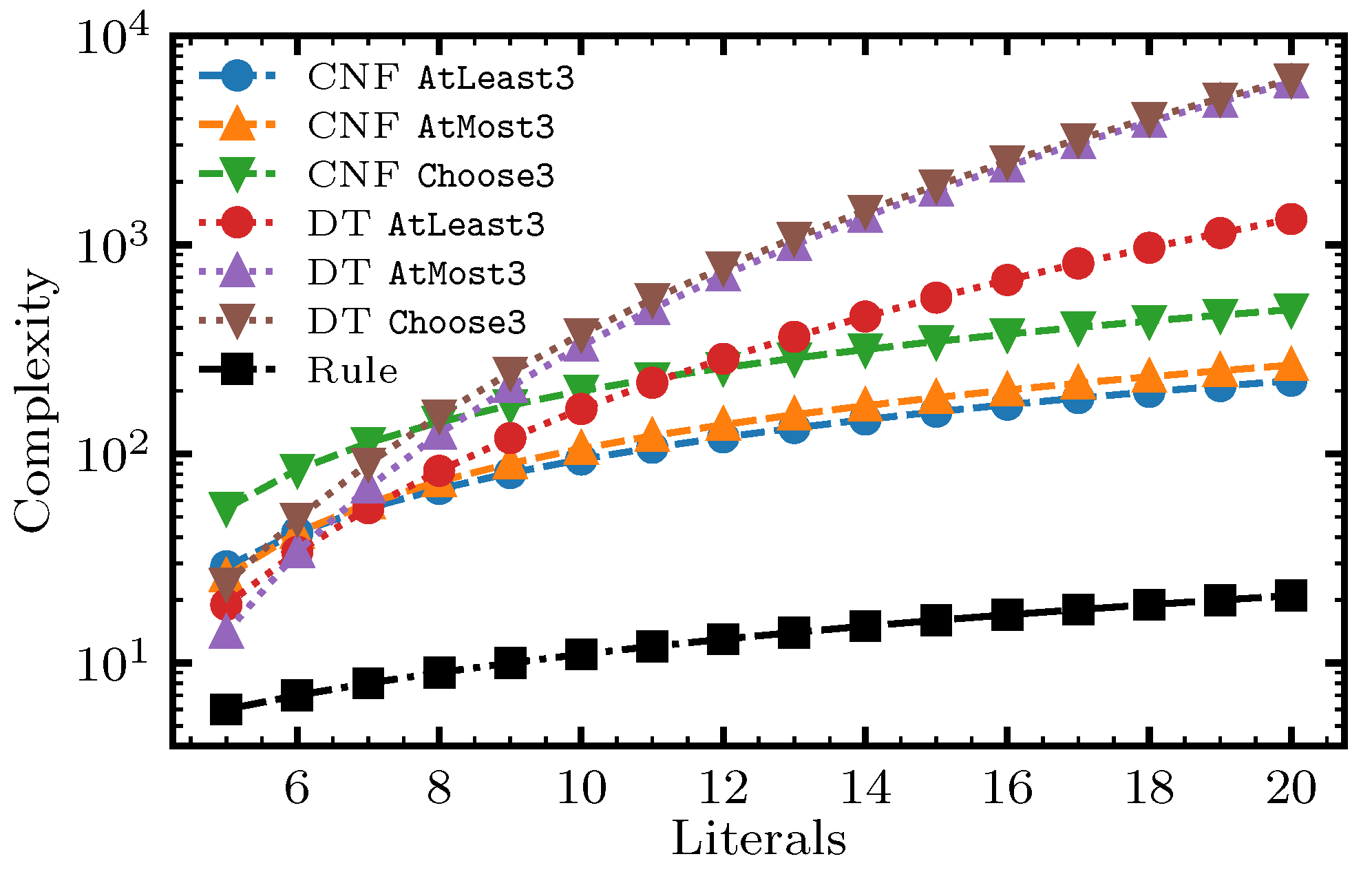
• Expressive Boolean formulas provide a more compact representation than decision trees and conjunctive normal form (CNF) rules for various examples.
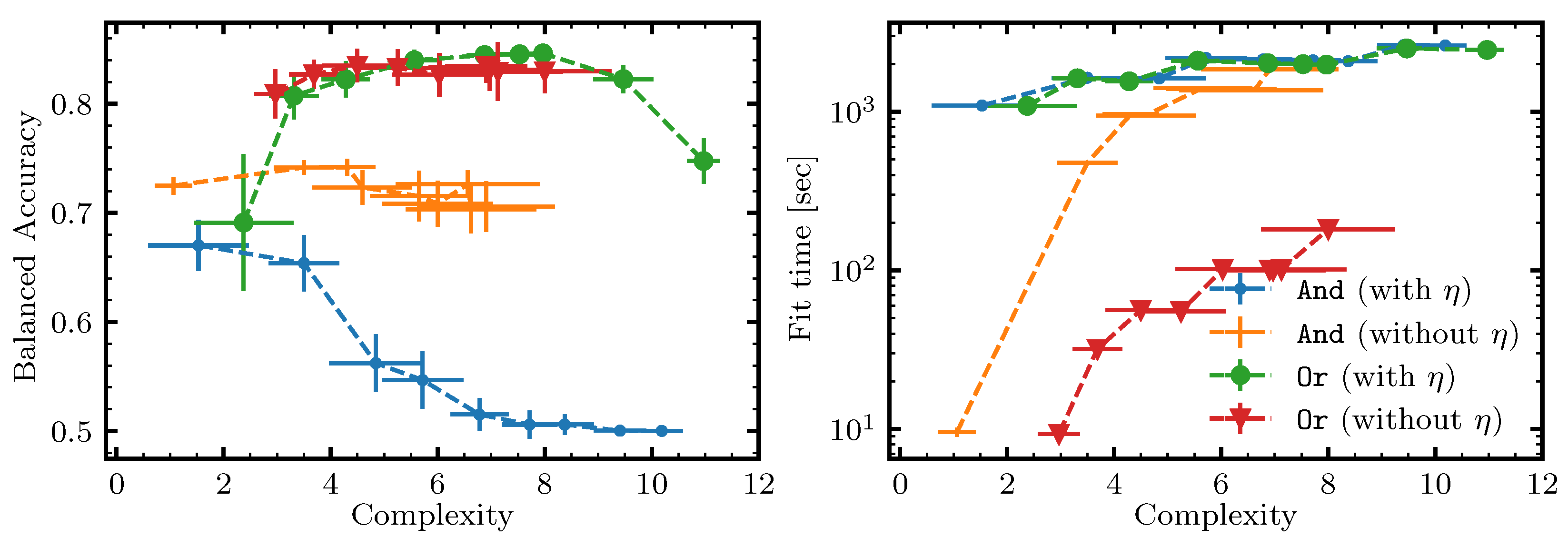
• Parameterized operators such as AtLeast are more expressive than non-parameterized operators such as Or.
• The native local rule classifier is competitive with the well-known alternatives considered in this work.
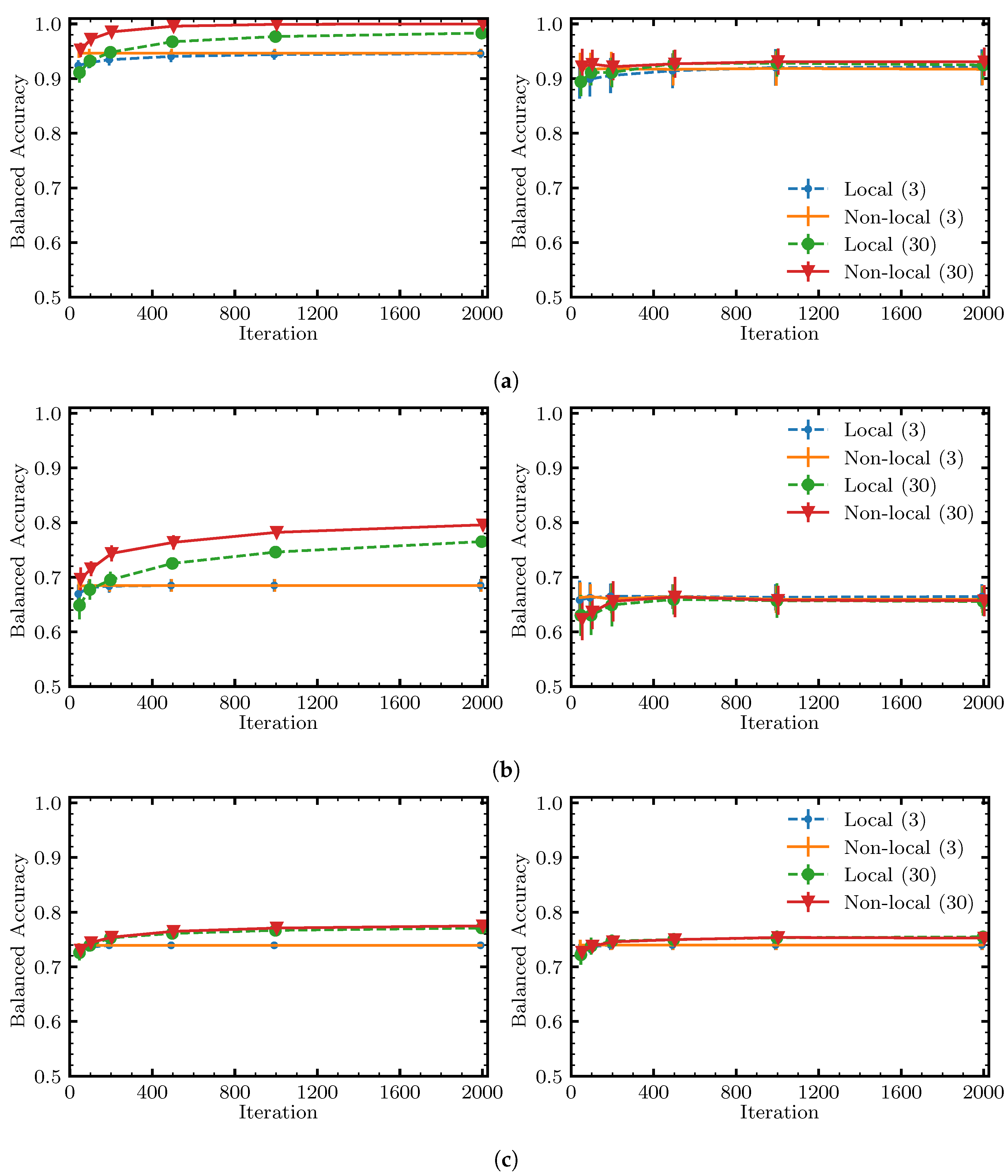
• The addition of non-local moves achieves similar results with fewer iterations. Therefore, using specialized or quantum hardware could lead to a significant speedup through the rapid proposal of non-local moves.

This paper is structured as follows. In Section 2, we review the related works, and in Section 3, we provide the problem definition, introduce expressive Boolean formulas, and justify their usage for explainable artificial intelligence (XAI). In Section 4, we describe the training of the classifier using a native local optimizer, including the idea and implementation of non-local moves. In Section 5, we formulate the problem of finding optimal depth-one rules as ILP and QUBO problems. In Section 6, we present and discuss our results, and in Section 7, we present our conclusions and discuss future directions.

2. Related Works

Explainable AI (XAI) is a branch of ML that aims to explain or interpret the decisions of ML models. Broadly speaking, there are two prevalent approaches to XAI, which we briefly review below:

Post hoc explanation of black-box models (Explainable ML)—Many state-of-the-art ML models, particularly in deep learning (DL), are huge, consisting of a large number of weights and biases, recently surpassing a trillion parameters [16]. These DL models are, by nature, difficult to decipher. The most common XAI approaches for these models provide post hoc explanations of black-box model decisions. These approaches are typically model agnostic and can be applied to arbitrarily complex models, such as the ones commonly used in DL.

Local explanation methods apply local approximations to groups of instances such as LIME [17] and SHAP [18] or to different feature sets such as MUSE [19]. Such methods often suffer from a lack of robustness and can typically be easily fooled by adversarial attacks [2,3].

Global explanation methods aim to mimic black-box models using interpretable models [20,21]. These methods benefit from the easy availability of additional data, by querying the black-box model. However, there is an issue of ambiguity—different interpretable models might yield the same high fidelity. Furthermore, since it is generally impossible to achieve perfect fidelity, the resulting model can deviate even further from the ground truth than the original black-box model.

Training interpretable models (Interpretable ML)—The definition of what constitutes an interpretable model is domain-specific and potentially user-specific. Nevertheless, many interpretable models have been studied. A few selected examples include rule lists [4], falling-rule lists [5], decision sets [6], scoring systems [7], and the more well-known decision trees and linear regression. There is an existing body of work on using specific Boolean formulas as ML models. For example, learning conjunctive/disjunctive normal form (CNF/DNF) rules using a MaxSAT (Maximum Satisfiability) solver [22,23], an ILP solver [24,25,26], or via LP relaxation [27].

There is a common belief that interpretable models yield less accurate results than more complex black-box models. However, in numerous cases, interpretable models have been shown to yield comparable results to black-box models [28], which is often the case for structured data with naturally meaningful features. Nonetheless, there may be cases in which interpretable models in fact do yield worse results. In those cases, a loss of accuracy might be a worthwhile concession in exchange for the additional trust that comes with an interpretable model.

Interpretable classifiers, including the classifiers described in this work, can be used as standalone interpretable models, or they can be used to explain black-box models. The main difference is in the origin of the labels—in the former, they would be the ground truth, whereas in the latter, they would be the output of the black-box model.

3. Research Methodology

In this section, we introduce our problem definition, the objective functions, and expressive Boolean formulas and justify their usage for XAI.

3.1. Problem Definition

We start with the definition of our problem.

Definition 1 (Rule Optimization Problem (ROP)). 

Given a binary feature matrix $\mathit{X}$ and a binary label vector $\mathit{y}$, the goal of the Rule Optimization Problem (ROP) is to find the optimum rule $R^{*}$ that balances the score S of the rule R on classifying the data, and the complexity of the rule C, which is given by the total number of features and operators in R. The complexity might, in addition, be bounded by a parameter $C^{\prime }$.

Mathematically, our optimization problem can be stated at a high level as:

$$\begin{array}{c}{R}^{\ast }={argmax}_R[S(R\left(\mathit{X}\right),\mathit{y})-\lambda C\left(R\right)]\hfill \\ \mathrm{s}.\mathrm{t}.C\left(R\right)\le C^{\prime },\hfill \end{array}$$

(1)

where R is any valid rule, $R^{\ast }$ is the optimized rule, S is the score, C is the complexity, $\mathit{X}$ is a binary matrix containing the input data, $\mathit{y}$ is a binary vector containing the corresponding labels, and $\lambda$ is a real number that controls the tradeoff between the score and the complexity. The solution to this problem is a single rule. Note that our problem definition is flexible and can accommodate different design decisions, which are described in more detail below.

3.2. Objectives

In this problem, we have two competing objectives: maximizing the performance and minimizing the complexity. The performance is measured by a given metric that yields a score S.

This problem could be solved by a multi-objective optimization solver, but we leave that for future work. Instead, we adopt two common practices in optimization:

• Combining multiple objectives into one—introducing a new parameter $\lambda \ge 0$ that controls the relative importance of the complexity (and, therefore, interpretability). The parameter $\lambda$ quantifies the drop in the score we are willing to accept to decrease the complexity by one. Higher values of $\lambda$ generally result in less complex models. We then solve a single-objective optimization problem with the objective function $S-\lambda C$, which combines both objectives into one hybrid objective controlled by the (use-specific) parameter $\lambda$.
• Constraining one of the objectives—introducing the maximum allowed complexity $C^{\prime }$ (also referred to as max_complexity) and then varying $C^{\prime }$ to achieve the desired result.

Normally, formulations include only one of these methods. However, we choose to include both in our formulation because the former method does not provide guidance on how to set $\lambda$, whereas the latter method provides tight control over the complexity of the rule at the cost of including an additional constraint. In principle, we prefer the tight control provided by setting $C^{\prime }$ since adding just one constraint is not a prohibitive price to pay. However, note that if $\lambda =0$, solutions that have an equal score but different complexity have the same objective function value. In reality, in most use cases, we expect that the lower complexity solution would be preferred. To indicate this preference to the solver, we recommend setting $\lambda$ to a small, nonzero value. Strategies for selecting $\lambda$ are outside the scope of this paper, but it is worth noting that the optimal choice of $\lambda$ should typically not exceed $1/C^{\prime }$. This is because, normally, the score $S\le 1$ and we want $\lambda C$ to be comparable to S. Therefore, $\lambda C\le \lambda C^{\prime }\le 1$, so $\lambda \le 1/C^{\prime }$. Regardless, in our implementation, users can set $C^{\prime }$, $\lambda$, both, or neither.

Without loss of generality, in this work, we mainly use balanced accuracy as the performance metric. Here, S is equal to the mean of the accuracy of predicting each of the two classes:

$$S=\frac{1}{2}\left(\frac{TP}{TP+FN}+\frac{TN}{TN+FP}\right),$$

(2)

where $TP$ is the number of true positives, $FN$ is the number of false negatives, $FP$ is the number of false positives, and $TN$ is the number of true negatives. Generalizations to alternative metrics are straightforward. For balanced datasets, balanced accuracy reduces to regular accuracy. The motivation for using this metric is that many datasets of interest are not well balanced.

A common use case is to explore the score vs. complexity tradeoff by varying $C^{\prime }$ or $\lambda$ over a range of values, producing a series of rules in the score–complexity space, as close as possible to the Pareto frontier.

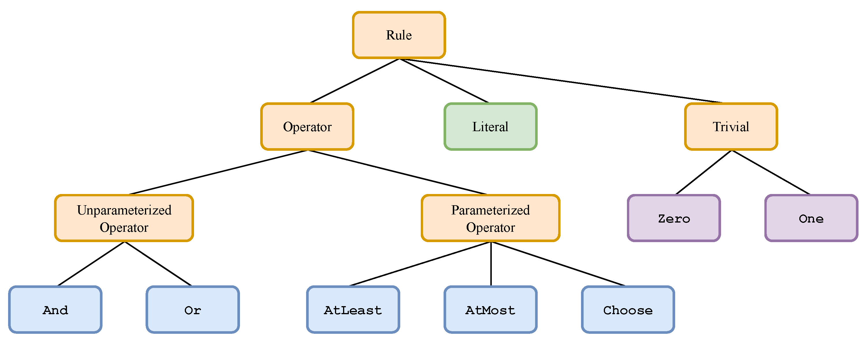
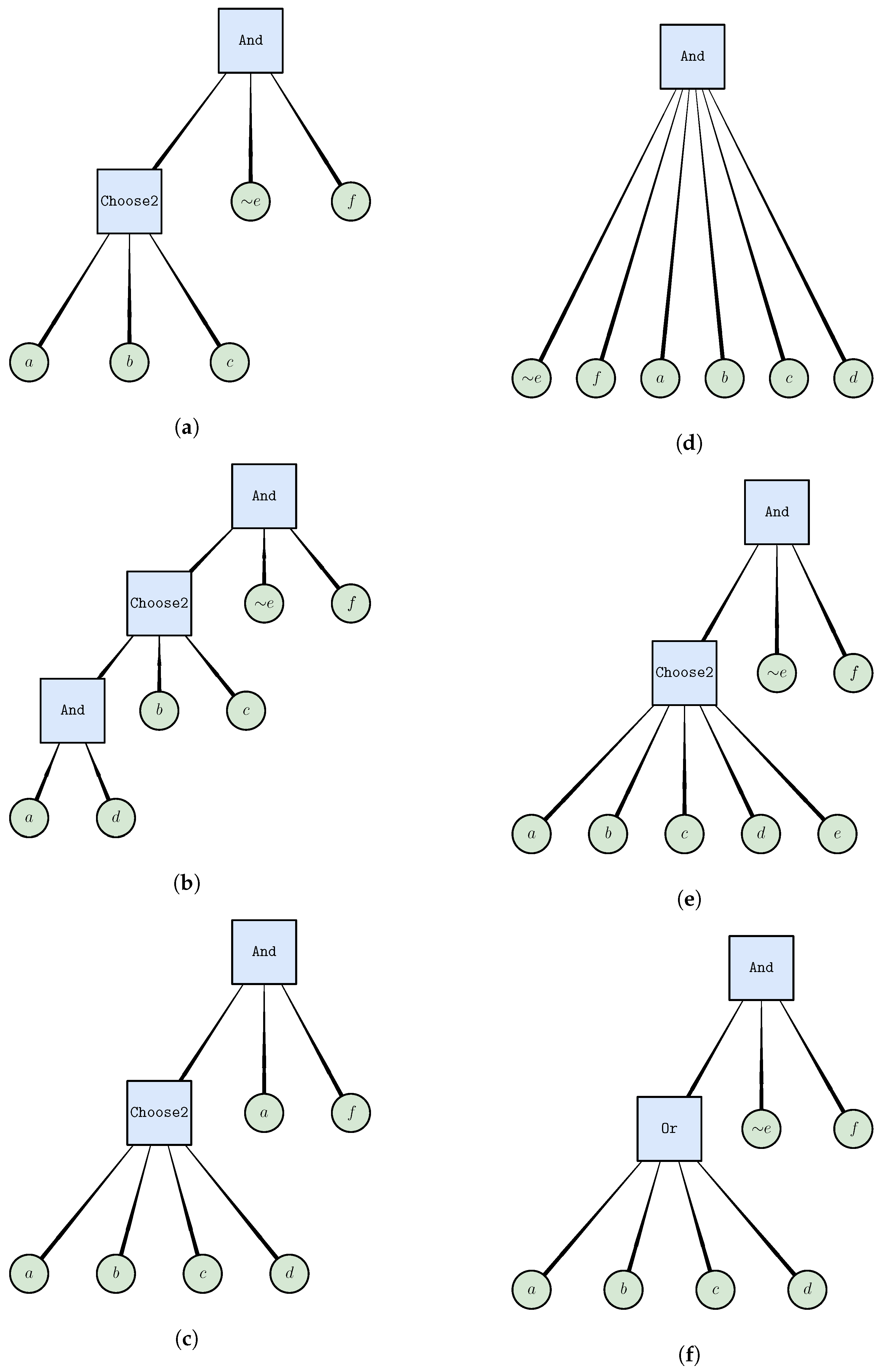
3.3. Rules as Expressive Boolean Formulas

The ROP (see Definition 1) can be solved over different rule definitions. In this work, we define the rules R to be Boolean formulas, specifically, expressive Boolean formulas. An expressive Boolean formula (henceforth, a “formula”), as we define it here, consists of literals and operators. Literals are variables $f_i$ or negated variables $\sim f_i$. Operators are operations that are performed on two or more literals, such as And($f_0,f_1,\sim f_2$) and Or($\sim f_0,f_1$). Some operators are parameterized, for example, AtLeast2($f_0,f_1,f_2$), which would return true only if at least two of the literals are true. Operators can optionally be negated as well. For simplicity, we consider negation to be a property of the respective literal or operator rather than being represented by a Not operator.

The inclusion of operators like AtLeast is motivated by the idea of (highly interpretable) checklists such as a list of medical symptoms that signify a particular condition. It is conceivable that a decision would be made using a checklist of symptoms, of which a minimum number would have to be present for a positive diagnosis. Another example is a bank trying to decide whether or not to provide credit to a customer.

In this work, we have included the operators Or, And, AtLeast, AtMost, and Choose (see Figure 1 for the complete hierarchy of rules). The definitions and implementation we have used are flexible and modular—additional operators could be added (such as AllEqual or Xor) or some could be removed.

It is convenient to visualize formulas as directed graphs (see Figure 2). The leaves in the graph are the literals that are connected with directed edges to the operator operating on them. To improve readability, we avoid crossovers by including a separate node for each literal, even if that literal appears in multiple places in the formula. Formally, this graph is a directed rooted tree. Evaluating a formula on given values of the variables can be accomplished by starting at the leaves, substituting the variable values, and then applying the operators until one reaches the top of the tree, referred to as the root.

We define the depth of a formula as the longest path from the root to any leaf (literal). For example, the formula in Figure 2 has a depth of two. We define the complexity as the total number of nodes in the tree, i.e., the total number of literals and operators in the formula. The same formula has a complexity of eight. This definition is motivated by the intuitive idea that adding literals or operators generally makes a given formula less interpretable. In this study, we are concerned with maximizing interpretability, which we do by minimizing complexity.

3.4. Motivation

In this section, we provide the motivation for our work using a few simple examples to illustrate how rigid rule-based classifiers and decision trees can require unreasonably complex models for simple rules.

Shallow decision trees are generally considered highly interpretable and can be trained fairly efficiently. However, it is easy to construct simple datasets that require very deep decision trees to achieve high accuracy. For example, consider a dataset with five binary features in which data rows are labeled as true only if at least three of the features are true. This is a simple rule that can be stated as AtLeast3($f_0,\cdots ,f_4$). However, training a decision tree on this dataset results in a large tree with 19 split nodes (see Figure 3). Despite encoding a simple rule, this decision tree is deep and difficult to interpret.

The prevalence of methods for finding optimal CNF (or equivalently, DNF) rules using MaxSAT solvers [22,23] or ILP solvers [24,25,26] suggests that one might use such a formula as the rule for the classifier. However, in this case, it is easy to construct simple datasets that require complicated rules. Consider the example above—the rule AtLeast3($f_0,\cdots ,f_4$) requires a CNF rule with 11 literals, 13 clauses, and a rule length of 29 (number of literals in all clauses).

Figure 4 shows several examples in which decision trees and CNF rules require a complicated representation of simple rules. The complexity C of a decision tree is defined here as the number of decision nodes. The complexity of a CNF formula is defined (conservatively) as the total number of literals that appear in the CNF formula (including repetitions). For the CNF rules, we also tried other encodings besides those indicated in the table (sorting networks [29], cardinality networks [30], totalizer [31], modulo totalizer [32], and modulo totalizer for k-cardinality [33]), all of which produced more complex formulas for this data. One can see that the decision tree encodings (“DT”) are the least efficient, followed by the CNF encodings (“CNF”), and finally, the expressive Boolean formulas (“Rule”) are by far the most efficient at encoding these rules.

4. The Components of the Solver

In this work, we propose to determine optimized expressive Boolean formulas via native local and non-local optimization. Here, “native” refers to optimization in the natural search space for the problem. This is in contrast to reformulating the problem in a fixed format such as MaxSAT, ILP, or QUBO, which would be difficult (if not impossible) and often requires searching a much larger space. A natural search space for this problem is the space of valid expressive Boolean formulas. Next, “local” refers to the exploration of the search space via a stochastic local search, i.e., by performing a series of moves that make relatively small changes to the current configuration [37]. “Non-local” optimization refers to the exploration of the search space via moves that change a larger part of the solution, a form of a large neighborhood search [38]. Below, we describe the native local optimizer and explain the idea of non-local moves and our specific implementation thereof.

To define a native local solver, we must define several components: the constraints and search space, how to generate the initial rules to start the optimization, the allowed local moves, how to evaluate the proposed rules, and the way the solver works. Below, we provide information about our choice for each of these components. However, other choices are possible for each of the components and might provide better results.

4.1. Constraints and Search Space

This problem can be posed as an unconstrained optimization problem. To do so, we must define the search space such that all candidate solutions are feasible. This search space is infinite if $C^{\prime }$ is not set. However, in this case, the solver focuses only on a small fraction of the search space due to the regularizing effect of $\lambda$. To observe this, note that $0\le S\le 1$ and $C\ge 1$. Thus, for a given value of $\lambda$, rules with $C>1/\lambda$ yield a negative objective function value, which is surely exceeded by at least one rule. Therefore, these rules would be avoided by the solver, or at least de-emphasized.

In principle, rules could involve no literals (“trivial rules”), a single literal, an operator that operates on two or more literals, and any nested combination of operators and literals. In practice, trivial rules and single-literal rules can be quickly checked exhaustively, and any reasonably complicated dataset would not provide high enough accuracy to be of interest. Therefore, we simplify our solver by excluding such rules. To check our assumptions (and as a useful baseline), our experiments include the results provided by the optimal single literal (feature) rule, as well as the optimal trivial rule (always one or always zero).

For parameterized operators, we constrain the search space so that it only includes sensible choices of the parameters. Namely, for AtMost, AtLeast, and Choose, we require that k is non-negative and is no larger than the number of literals under the operator. These constraints are fulfilled through construction by picking initial solutions and proposing moves that take them into account.

4.2. Generating Initial Rules

The initial rules are constructed by choosing between two and $C^{\prime }-1$ literals randomly (without replacement). Literals are chosen for negation via a coin flip. Once the literals have been chosen, an operator and valid parameter (if the operator chosen is parameterized) are selected randomly. These generated rules are of depth-one—additional depth is explored by subsequent moves.

4.3. Generating Local Moves

Feasible local moves are found by rejection sampling as follows. A node (literal or operator) in the current rule is chosen at random, and a move type is chosen by cycling over the respective move types for the chosen literal/operator. Next, a random move of the chosen type is drawn. If the random move is invalid, the process is restarted, until a valid move is found (see Algorithm 1). Typically, only a few iterations are needed, at most.

Algorithm 1 The function that proposes local moves—propose_local_move(). This function selects a node (an operator or a literal) randomly while cycling through the move types and then attempts to find a valid local move for that node and move type. The process is restarted if needed until a valid local move is found, a process that is referred to as “rejection sampling”.

literal_move_types=cycle({"remove_literal","expand_literal_to_operator",                                                    "swap_literal"}) operator_move_types=cycle({"remove_operator","add_literal","swap_operator"})   def propose_local_move(current_rule):     all_operators_and_literals = current_rule.flatten()       proposed_move = None     while proposed_move is None:         target = random.choice(all_operators_and_literals)           if isinstance(target, Literal):            move_type = next(literal_move_types)         else:            move_type = next(operator_move_types)           proposed_move = get_random_move(move_type, target)       return proposed_move

The literal move types we have implemented are as follows (see Figure 5a–c):

• Remove literal—removes the chosen literal but only if the parent operator would not end up with fewer than two subrules. If the parent is a parameterized operator, it adjusts the parameter down (if needed) so that it remains valid after the removal of the chosen literal.
• Expand literal to operator—expands a chosen literal to an operator, moving a randomly chosen sibling literal to that new operator. It proceeds only if the parent operator includes at least one more literal. If the parent is a parameterized operator, it adjusts the parameter down (if needed) so that it remains valid after the removal of the chosen literal and the sibling literal.
• Swap literal—replaces the chosen literal with a random literal that is either the negation of the current literal or is a (possibly negated) literal that is not already included under the parent operator.

Figure 5. Local move types. Moves on literals are shown in (a–c) and moves on operators in (d–f). All moves are relative to the initial rule shown in Figure 2. (a) Remove literal d. (b) Expand literal a to operator And. (c) Swap literal $\sim e$ for a. (d) Remove operator Choose2. (e) Add literal e to operator Choose2. (f) Swap operator Choose2 for Or.

Figure 5. Local move types. Moves on literals are shown in (a–c) and moves on operators in (d–f). All moves are relative to the initial rule shown in Figure 2. (a) Remove literal d. (b) Expand literal a to operator And. (c) Swap literal $\sim e$ for a. (d) Remove operator Choose2. (e) Add literal e to operator Choose2. (f) Swap operator Choose2 for Or.

The operator move types we have implemented are as follows (see Figure 5d–f):

• Remove operator—removes an operator and any operators and literals under it. It only proceeds if the operator has a parent (i.e., it is not the root) and if the parent operator has at least three subrules, such that the rule is still valid after the move has been applied.
• Add literal to operator—adds a random literal (possibly negated) to a given operator, but only if that variable is not already included in the parent operator.
• Swap operator—swaps an operator for a randomly selected operator and a randomly selected parameter (if the new operator is parameterized). It proceeds only if the new operator type is different or if the parameter is different.

4.4. Evaluation of Rules

The “goodness” of a rule is defined by the objective function in Equation (1), i.e., as $S-\lambda C$. To calculate the objective function, we must evaluate the rule with respect to the given data rows. The evaluation yields a Boolean prediction for each data row. Evaluating the metric on the predictions and respective labels results in a score S. The complexity of a rule C is a function only of the rule’s structure and does not depend on the inputs. Therefore, the computational complexity of calculating the objective function is dominated by the rule evaluation, which is linear in both the number of samples and the rule complexity.

The evaluation of literals is immediate because the result is simply equal to the respective feature (data column) or the complement of that feature. The evaluation of operators is accomplished by evaluating all the subrules and then applying the operator to the result. Evaluation is usually performed on multiple rows at once. For this reason, it is far more efficient to implement evaluation using vectorization, as we have done. In fact, for large datasets, it might be beneficial to parallelize this calculation because it is trivially parallelizable (over the data rows). In addition, evaluation in the context of a local solver could likely be made far more efficient by memoization, i.e., storing the already evaluated subrules so that they can be looked up rather than re-evaluated.

4.5. The Native Local Solver

The solver starts by generating a new random rule num_starts times, which diversifies the search and is embarrassingly parallelizable. We have implemented a simulated annealing [39] solver, but other stochastic local search solvers [37] could also be implemented (e.g., greedy, tabu, etc.). Each start begins by generating an initial random rule and continues with the proposal of num_iterations local moves. Moves are accepted based on a Metropolis criterion, such that the acceptance probability of a proposed move $P(\Delta F,T)=min(1,e^{-\Delta F/T})$ depends only on the objective function change $\Delta F$ and temperature T. Initially, the temperature is high, leading to most moves being accepted (exploration), regardless of the value of $\Delta F$. The temperature is decreased on a geometrical schedule, such that in the latter stages of each start, the solver accepts only descending or “sideways” moves—moves that do not change the objective function (exploitation), i.e., moves for which $\Delta F\le 0$ (see Figure 6 for an example run).

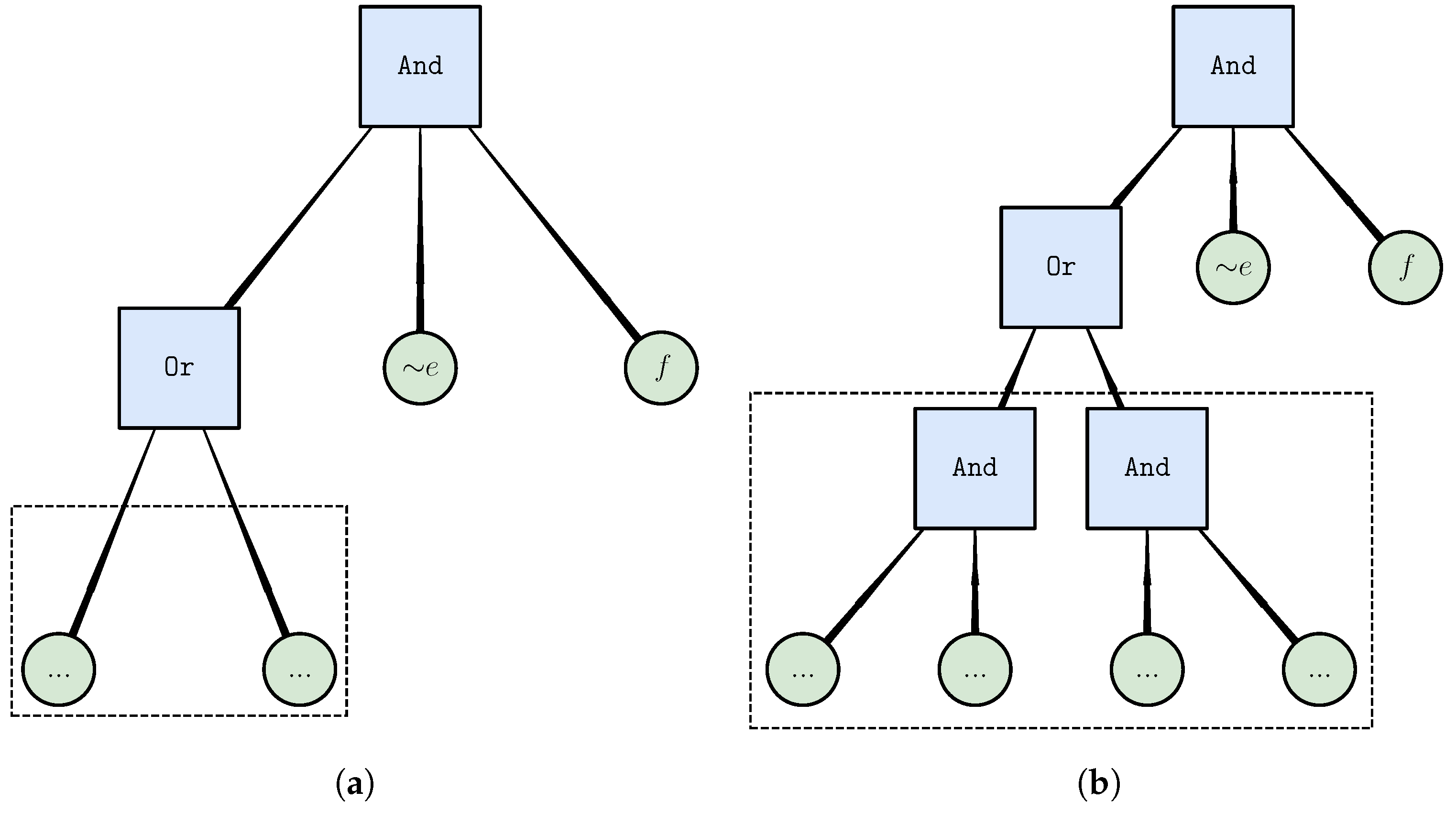
4.6. Non-Local Moves

The local native optimizer described above searches the formula space by making small local moves. It is also possible to perform larger, non-local moves. Such moves are more expensive computationally, but they have the potential to improve the objective function more drastically by extending the range of the otherwise local search, as well as allowing the solver to escape local minima. In this section, we describe ways of proposing good non-local moves that are compatible with, and inspired by, quantum algorithms for optimization that might show a speedup compared to classical algorithms, namely algorithms for solving QUBO and ILP problems [41,42,43,44].

The basic idea behind the proposed non-local moves is to make a move that optimizes an entire subtree of the current formula. Given a randomly selected target node (an operator or literal) and a new operator, we assign the new operator to the target node and optimize the subtree beneath it.

The optimized subtree could be of depth one (i.e., an operator with literals under it) or depth two (i.e., an operator with other operators and literals under it, with literals under the secondary operators). The optimization of the subtree could be limited to a particular subset of the possible subtrees, which can occur when using fixed-format optimizers. An example of a depth-two tree of a fixed format is a DNF rule, i.e., an Or of Ands. We refer to the subtree optimization move as swap node with a subtree of depth d (see Figure 7a,b), and in this work, we focus on the $d=1$ case.

To perform the optimization over the subtree T, we need to determine the effective input data and labels for the subtree optimization problem, ${\mathit{X}}^{\prime }$ and ${\mathit{y}}^{\prime }$, respectively. We now use the notation $R(T\left(x_i\right),x_i)$ to highlight that the evaluation of the rule can be regarded as the result of evaluating the subtree and then evaluating the rest of the rule given the result of the subtree evaluation. For each data row (sample) $x_i$ we evaluate the rule $R(T\left(x_i\right),x_i)$ twice by first substituting $T\left(x_i\right)=0$ and then $T\left(x_i\right)=1$. If the result is the same in both cases, it is predetermined, and hence the sample $x_i$ does not contribute to the score of any proposed subtree T. If the result is different, we set $y_i^{\prime }$ to the value that causes the classification to be correct, i.e., such that $R\left(x_i\right)=y_i$, and add the corresponding sample to ${\mathit{X}}^{\prime }$. Note that it is guaranteed in this case that one of these options classifies the sample correctly because in this case, we have two different outputs, which cover all of the possible outputs (for binary classification). The subtree score is then calculated only over the labels that are not predetermined, i.e., the effective labels. The complexity of the subtree $C\left(T\right)$ is calculated in the same way it is calculated for the complete rule.

To determine the non-local move, we solve an optimization problem that is determined by fixing $R/T_0$ (i.e., everything that is not the target node or a descendant of it) in Equation (1) and discarding constants, where $T_0$ is the target subtree (prior to optimization). In particular, we have

$$\begin{array}{c}{T}^{\ast }={argmax}_T[S(T\left({\mathit{X}}^{\prime }\right),{\mathit{y}}^{\prime })-\lambda C\left(T\right)]\hfill \\ \mathrm{s}.\mathrm{t}.C\left(T\right)\le C^{\prime }-[C\left(R\right)-C\left(T_0\right)],\hfill \end{array}$$

(3)

where ${\mathit{X}}^{\prime }$ and ${\mathit{y}}^{\prime }$ are the input data and effective subtree labels for the non-predetermined data rows, respectively, T is any valid subtree, and $T^{\ast }$ is the optimized subtree (i.e., the proposed non-local move).

In practice, we must also constrain the complexity of the subtree from below because otherwise, the optimized subtree could cause the rule to be invalid. For this reason, if the target is the root, we enforce $\mathtt{min}\_\mathtt{num}\_\mathtt{literals}=2$ because the root operator must have two or more literals. If the target is not the root, we enforce $\mathtt{min}\_\mathtt{num}\_\mathtt{literals}=1$ to enable the replacement of the subtree with a single literal (if beneficial). The ILP and QUBO formulations we present in Section 5 do not include this lower bound on the number of literals for simplicity, but its addition is trivial.

Yet another practical consideration is that we want to propose non-local moves quickly to keep the total solving time within the allotted limit. One way of trying to achieve this is to set a short timeout. However, the time required to construct and solve the problems is dependent on the number of non-determined samples. If the number of samples is large and the timeout is short, the best solution found might be of poor quality. With this in mind, we define a parameter named max_samples, which controls the maximum number of samples that can be included in this optimization problem. This parameter controls the tradeoff between the effort required to find a good non-local move to propose and the speed with which such a move can be constructed. Even with this parameter in place, the time required to find the optimal solution can be significant (for example minutes or more), so we utilize a short timeout.

4.7. Putting It All Together

Now that we have described the idea of the non-local moves at a high level, we describe the way we have incorporated them into the native local solver in more detail. In Algorithm 2, the pseudo-code for the simulated annealing native local solver with non-local moves is presented. Non-local moves are relatively expensive to calculate and thus should be used sparingly. Moreover, non-local moves are fairly exploitative (as opposed to exploratory), so in the context of simulated annealing, proposing such moves at the beginning of the optimization would not help convergence and, therefore, would be a waste of computational resources. With these points in mind, we define a burn-in period num_iterations_burn_in for each start in which no non-local moves are proposed. After the burn-in period, non-local moves are proposed only if a certain number of iterations (referred to as the patience) has passed without any improvements due to proposing local moves. A short example run is presented in Figure 8, showing the evolution of the objective function over multiple starts, how the non-local moves are introduced after an initial burn-in period, and their ability to measurably improve the objective function, albeit with occasional failures.

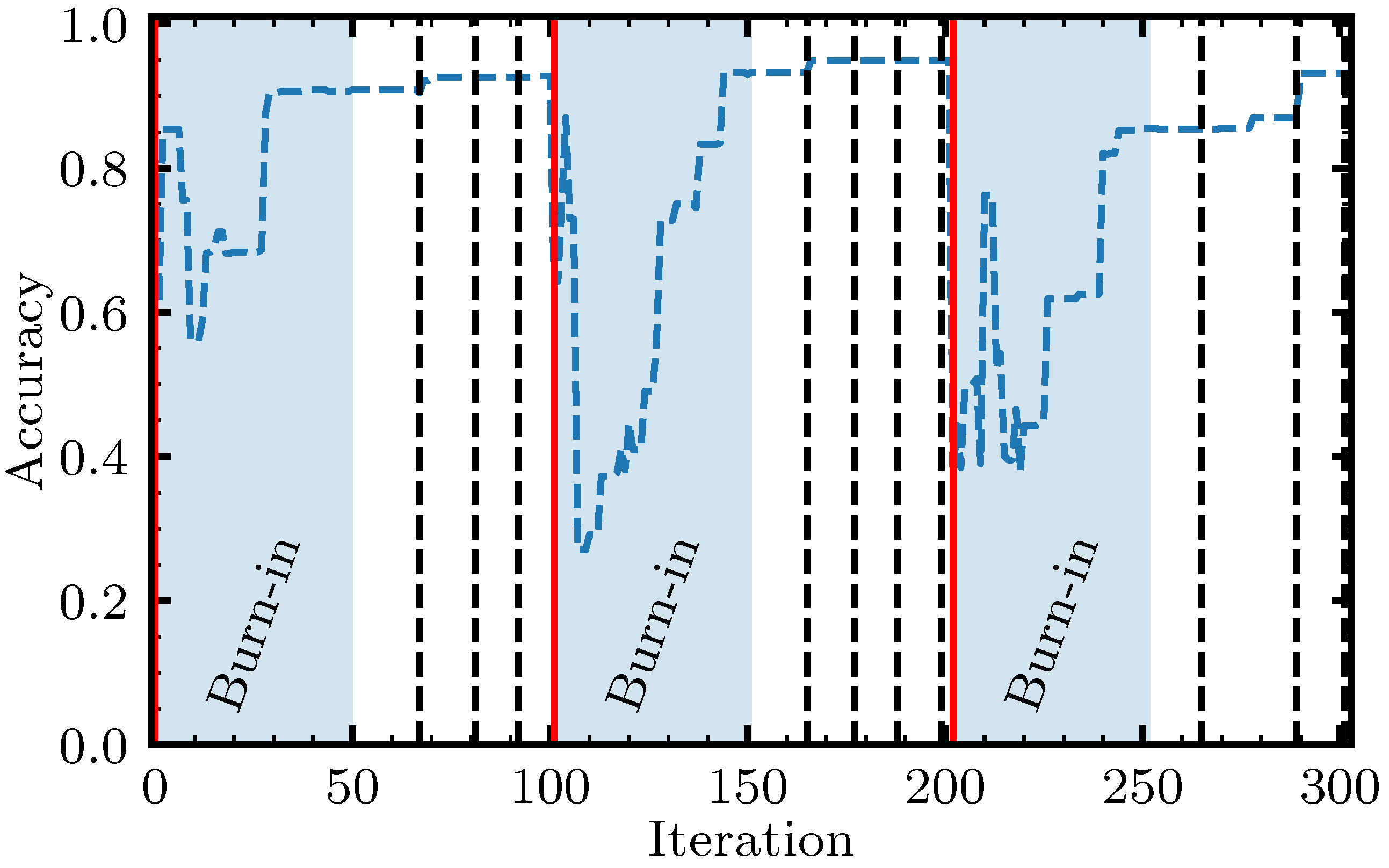
Algorithm 2 The pseudo-code for our native local solver with non-local moves. The solver executes num_starts starts, each with num_iterations iterations. In each start, a random initial rule is constructed and then a series of local (see Algorithm 1) and non-local moves (see Section 4.6) are proposed and accepted based on the Metropolis criterion. Non-local moves are introduced only after initial num_iterations_burn_in iterations and only if there have been no improvements over patience iterations. Both the initial rule and the proposed moves are constructed so that the current rule is always feasible and, in particular, has a complexity no higher than max_complexity. Non-local moves replace an existing literal or operator with a subtree, optimized over a randomly selected subset of the data of size max_samples. The solver returns the best rule found. Some details are omitted due to a lack of space.

def solve(X, y, max_complexity, num_starts,           num_iterations, num_iterations_burn_in, patience):      best_score = -inf      best_rule = None      for start in range(num_starts):          is_patience_exceeded = False          current_rule = generate_initial_rule(X, max_complexity)          current_score = score(current_rule, X, y)           for iteration in range(num_iterations):             T = update_temperature()             if iteration > num_iterations_burn_in and is_patience_exceeded:                 proposed_move = propose_non_local_move(current_rule, max_samples)             else:                 proposed_move = propose_local_move(current_rule)               proposed_move_score = score(proposed_move, X, y)             dE = proposed_move_score - current_score             accept = dE >= 0 or random.random() < exp(dE/T)               if accept:                 current_score = proposed_move_score                 current_rule = proposed_move                   if current_score > best_score:                     best_score = current_score                     best_rule = deepcopy(current_rule)                   is_patience_exceeded = update_patience_exceeded(patience)     return best_rule

5. Depth-One ILP and QUBO Formulations

In this section, we formulate the problem of finding optimal depth-one rules as an ILP or QUBO problem, with various operators at the root. We use these formulations in two ways: (1) to find optimized depth-one rules that form the basis of standalone classifiers, and (2) to find good non-local moves in the context of a native local solver, which periodically proposes non-local moves.

We start by following [27], which explains how to formulate the search for the optimal Or, And, and AtLeast rules as ILP problems. Our contributions here are as follows:

• The addition of negated features.
• Design of even-handed formulations (unbiased toward positive/negative samples) and the addition of class weights.
• Correction of the original formulation for AtLeast and generalizations to the AtMost and Choose operators.
• Direct control over the score/complexity tradeoff by constraining the number of literals.

We then explain how to translate these formulations into QUBO formulations. Finally, we describe how the constraints can be softened, thereby significantly reducing the search space.

5.1. Formulating the Or Rule as an ILP

We start by observing that the rule y = Or($f_0,f_1$) can be equivalently expressed as:

$$\begin{array}{cc}{f}_0+f_1\ge 1& \mathrm{for}y=1\phantom{.}\\ f_0+f_1=0& \mathrm{for}y=0.\end{array}$$

(4)

We can then define an optimization problem to find the smallest subset of features $f_i$ to include in the Or rule to achieve perfect accuracy:

$$\begin{array}{cccc}\hfill & min\hfill & \hfill & {\left|\right|\mathit{b}\left|\right|}_0\hfill \\ \hfill & \mathrm{s}.\mathrm{t}.\hfill & \hfill & {\mathit{X}}_{\mathit{P}}\mathit{b}\ge \mathbf{1}\hfill \\ \hfill & \hfill & & {\mathit{X}}_{\mathit{N}}\mathit{b}=\mathbf{0},\hfill \\ \hfill & \hfill & & \mathit{b}\in {\{0,1\}}^m\hfill \end{array}$$

(5)

where $\mathit{b}$ is a vector of indicator variables, indicating whether each feature should be included in the rule (i.e., $b_i=1$ if feature $f_i$ is included and $b_i=0$ otherwise), ${\mathit{X}}_{\mathit{P}}$ is a matrix containing only the rows labeled as “positive” ($y=1$), ${\mathit{X}}_{\mathit{N}}$ is a matrix containing only the rows labeled as “negative” ($y=0$), and $\mathbf{0}$ and $\mathbf{1}$ are vectors containing only zeros and ones, respectively.

We extend this formulation by adding the possibility to include negated features in the rule. While this could be accomplished simply by adding the negated features to the input data $\mathit{X}$, thereby doubling the size of this matrix, it may be more efficient to include the negation in the formulation. To accomplish this, we add a vector of the indicator variables $\tilde{\mathit{b}}$, indicating whether each negated feature should be included in the rule. We then replace $\mathit{X}\mathit{b}\to \mathit{X}\mathit{b}+\tilde{\mathit{X}}\tilde{\mathit{b}}$, noting that $\tilde{\mathit{X}}=\mathbf{1}-\mathit{X}$ (where $\mathbf{1}$ is now a matrix of ones) since a binary variable $v\in \{0,1\}$ is negated by $1-v$. Therefore, we have:

$$\mathit{X}\mathit{b}\to \mathit{X}\mathit{b}+\tilde{\mathit{X}}\tilde{\mathit{b}}=\mathit{X}\mathit{b}+(\mathbf{1}-\mathit{X})\tilde{\mathit{b}}=\mathit{X}(\mathit{b}-\tilde{\mathit{b}})+\left|\right|\tilde{\mathit{b}}{\left|\right|}_0,$$

where $\left|\right|\tilde{\mathit{b}}{\left|\right|}_0$ is the sum over the entries of $\tilde{\mathit{b}}$. By substituting the above into Equation (5) and adding a corresponding term for $\tilde{\mathit{b}}$ to the objective function, we find that:

$$\begin{array}{cccc}\hfill & min\hfill & \hfill & {\left|\right|\mathit{b}\left|\right|}_0+\left|\right|\tilde{\mathit{b}}{\left|\right|}_0\hfill \\ \hfill & \mathrm{s}.\mathrm{t}.\hfill & \hfill & {\mathit{X}}_{\mathit{P}}(\mathit{b}-\tilde{\mathit{b}})+\left|\right|\tilde{\mathit{b}}{\left|\right|}_0\ge \mathbf{1}\hfill \\ \hfill & \hfill & & {\mathit{X}}_{\mathit{N}}(\mathit{b}-\tilde{\mathit{b}})+\left|\right|\tilde{\mathit{b}}{\left|\right|}_0=\mathbf{0}\hfill \\ \hfill & \hfill & & \mathit{b},\tilde{\mathit{b}}\in {\{0,1\}}^m.\hfill \end{array}$$

(6)

In practice, we typically do not expect to be able to achieve perfect accuracy. With this in mind, we introduce a vector of “error” indicator variables $\mathit{\eta }$, indicating whether each data row is misclassified. When the error variable corresponding to a particular sample is 1, the corresponding constraint is always true by construction, effectively deactivating that constraint. Accordingly, we change our objective function so that it minimizes the number of errors. To control the complexity of the rule, we add a regularization term, as well as an explicit constraint on the number of literals. Finally, to deal with unbalanced datasets, we allow the positive and negative error terms to be weighted differently:

$$\begin{array}{cccc}\hfill & min\hfill & \hfill & (w_P\left|\right|{\mathit{\eta }}_{\mathit{P}}{\left|\right|}_0+w_N\left|\right|{\mathit{\eta }}_{\mathit{N}}{\left|\right|}_0{)+\lambda (\left|\right|\mathit{b}\left|\right|}_0+\left|\right|\tilde{\mathit{b}}{\left|\right|}_0)\hfill \\ \hfill & \mathrm{s}.\mathrm{t}.\hfill & \hfill & {\mathit{X}}_{\mathit{P}}(\mathit{b}-\tilde{\mathit{b}})+\left|\right|\tilde{\mathit{b}}{\left|\right|}_0+{\mathit{\eta }}_{\mathit{P}}\ge \mathbf{1}\hfill \\ \hfill & \hfill & & {\mathit{X}}_{\mathit{N}}(\mathit{b}-\tilde{\mathit{b}})+\left|\right|\tilde{\mathit{b}}{\left|\right|}_0-{\mathit{\eta }}_{\mathit{N}}{m}^{\prime }\le \mathbf{0}\hfill \\ \hfill & & \hfill & {\left|\right|\mathit{b}\left|\right|}_0+\left|\right|\tilde{\mathit{b}}{\left|\right|}_0\le m^{\prime }\hfill \\ \hfill & \hfill & & \mathit{b},\tilde{\mathit{b}}\in {\{0,1\}}^m,\mathit{\eta }\in {\{0,1\}}^n,\hfill \end{array}$$

(7)

where $m^{\prime }$ (also referred to as max_num_literals) is the maximum number of literals allowed; $m^{\prime }\le m$, where m is the number of features; and $w_P$ and $w_N$ are the positive and negative class weights, respectively. The default choice for the class weights is to make them inversely proportional to the fraction of samples of each respective class. In this work, we set $w_P=n/\left(2n_P\right)$ and similarly, $w_N=n/\left(2n_N\right)$, where $n_P$ is the number of positive samples, $n_N$ is the number of negative samples, and n is the total number of samples ($n=n_P+n_N$).

By inspecting Equation (7), one can see that when a positive data row is misclassified ($\eta =1$), the first constraint is always fulfilled. This is because the left-hand side of that constraint is then the sum of one plus a non-negative number, which is always larger than or equal to one. Similarly, when a negative data row is misclassified, the second constraint is always satisfied. This is because the left-hand side of that constraint consists of a number that is bound from above by $m^{\prime }$ from which $m^{\prime }$ is subtracted, which is surely negative or zero. Note that this second constraint for the negative samples was previously an equality constraint (in Equation (6)), which was changed to an inequality constraint to make the “deactivation” (for $\eta =1$) work.

5.2. Formulating the And Rule as an ILP

In the previous section, we described the ILP formulation for the Or operator. In this section, we show how this formulation can be extended to the And operator. It is instructive to first consider why it is useful to go beyond the Or rules at all and what is the exact nature of the relationship between Or and And rules in this context.

We note that De Morgan’s laws (which we use below) guarantee that every Or rule has an equivalent $\sim \mathtt{And}$ rule (and similarly for And and $\sim \mathtt{Or}$). The relation between the distribution of the different rules is apparent in Figure 9, where we plot the score landscape for both single- and double-feature rules. In particular, the distribution of Or clearly matches the distribution of ∼And (and similarly, for And and ∼Or), as expected. More importantly for us, the distribution of Or is clearly very different from the distribution of And, motivating the introduction of the latter. Similarly, the distribution of non-negated single-feature rules is clearly very different from the distribution of negated single-feature rules, again motivating the inclusion of negated features. As an aside, note the reflection symmetry in both plots, which is due to the identity $S\left(R\right)=1-S(\sim R)$.

The best (optimal) rules for each distribution are presented in

Table 1. The best (optimal) rules for single- and double-feature rules for the full Breast Cancer dataset. “Type” is the type of rule, “Rules” is the number of rules of that rule type, “Accuracy” is regular accuracy (the metric used for this table), and “Rule” is one of the optimal rules for the respective rule type. Negations of features are post-processed out for readability by reversing the relationship in the respective feature name (e.g., $\sim a>3\to a\le 3$).

Type	Rules	Accuracy	Rule
f	300	0.647	mean fractal dimension > 0.0552
∼f	300	0.914	worst perimeter ≤ 108.9364
Or	179,400	0.931	Or(worst concave points ≤ 0.1091, worst area ≤ 719.6364)
∼Or	179,400	0.944	∼Or(worst concave points > 0.1563, worst area > 988.6818)
And	179,400	0.944	And(worst concave points ≤ 0.1563, worst area ≤ 88.6818)
∼And	179,400	0.931	∼And(worst concave points > 0.1091, worst area > 719.6364)

. The best And rule is significantly better than the best Or rule in this case, clearly motivating its inclusion. Furthermore, the reason for including negated features is clear when comparing the best single-feature rule scores.

As a final motivational observation, we note that as max_num_literals is increased, Or rules generally tend to produce false positives (since additional features tend to push more outputs to one), whereas And rules generally tend to produce false negatives (since additional features tend to push more outputs to zero). Different use cases might lend themselves to either of these operators. However, both of these operators are fairly rigid, a point that is mitigated by the introduction of parameterized operators (see Section 5.3) and higher depth rules, as found by the native local solver (see Section 4).

To formulate the And operator, we use De Morgan’s laws. Namely, starting from Equation (7), we swap $\mathit{b}\leftrightarrow \tilde{\mathit{b}}$, ${\mathit{\eta }}_{\mathit{N}}\leftrightarrow {\mathit{\eta }}_{\mathit{P}}$, and ${\mathit{X}}_{\mathit{N}}\leftrightarrow {\mathit{X}}_{\mathit{P}}$ to find that:

$$\begin{array}{cccc}\hfill & min\hfill & \hfill & (w_P\left|\right|{\mathit{\eta }}_{\mathit{P}}{\left|\right|}_0+w_N\left|\right|{\mathit{\eta }}_{\mathit{N}}{\left|\right|}_0{)+\lambda (\left|\right|\mathit{b}\left|\right|}_0+\left|\right|\tilde{\mathit{b}}{\left|\right|}_0)\hfill \\ \hfill & \mathrm{s}.\mathrm{t}.\hfill & \hfill & {\mathit{X}}_{\mathit{N}}(\tilde{\mathit{b}}-\mathit{b})+{\left|\right|\mathit{b}\left|\right|}_0+{\mathit{\eta }}_{\mathit{N}}\ge \mathbf{1}\hfill \\ \hfill & \hfill & & {\mathit{X}}_{\mathit{P}}(\tilde{\mathit{b}}-\mathit{b})+{\left|\right|\mathit{b}\left|\right|}_0-{\mathit{\eta }}_{\mathit{P}}{m}^{\prime }\le \mathbf{0}\hfill \\ \hfill & & \hfill & {\left|\right|\mathit{b}\left|\right|}_0+\left|\right|\tilde{\mathit{b}}{\left|\right|}_0\le m^{\prime }\hfill \\ \hfill & \hfill & & \mathit{b},\tilde{\mathit{b}}\in {\{0,1\}}^m,\mathit{\eta }\in {\{0,1\}}^n.\hfill \end{array}$$

(8)

5.3. Extending the ILP Formulation to Parameterized Operators

So far, we have shown how the problem of finding an optimal depth-one rule with Or and And operators in the root can be formulated as an ILP. Here, we extend these formulations to the parameterized operators AtLeast, AtMost, and Choose. This is motivated by the hypothesis that the additional parameter in these operators could provide additional expressivity, which could translate into better results for particular datasets, at least for some values of max_num_literals.

We probe this idea in an experiment, in which we vary max_num_literals over the full possible range for the Breast Cancer dataset, as shown in Figure 10. In this experiment, we fix max_num_literals=min_num_literals to expose the true objective value over the full range. One can clearly see that the additional expressivity of the parameterized operators allows them to maintain a higher accuracy over most of the possible range for both the training and test samples. For the unparameterized operators, we observe significantly reduced performance at high max_num_literals, explained by the fact that eventually, the solver runs out of features that can be added and still improve the score. For the parameterized operators, this limitation is mitigated by adjusting the corresponding parameter.

To formulate the AtLeast operator, we modify Equation (4) such that the rule y = AtLeastk($f_0,f_1$) can be equivalently expressed as

$$\begin{array}{ccc}\hfill & f_0+f_1\ge k\hfill & \mathrm{for}y=1\phantom{.}\hfill \\ \hfill & f_0+f_1\le k-1\hfill & \mathrm{for}y=0.\hfill \end{array}$$

(9)

Accordingly, we modify Equation (7) to obtain the ILP formulation for AtLeast:

$$\begin{array}{cccc}\hfill & min\hfill & \hfill & (w_P\left|\right|{\mathit{\eta }}_{\mathit{P}}{\left|\right|}_0+w_N\left|\right|{\mathit{\eta }}_{\mathit{N}}{\left|\right|}_0{)+\lambda (\left|\right|\mathit{b}\left|\right|}_0+\left|\right|\tilde{\mathit{b}}{\left|\right|}_0)\hfill \\ \hfill & \mathrm{s}.\mathrm{t}.\hfill & \hfill & {\mathit{X}}_{\mathit{P}}(\mathit{b}-\tilde{\mathit{b}})+\left|\right|\tilde{\mathit{b}}{\left|\right|}_0+{\mathit{\eta }}_{\mathit{P}}{m}^{\prime }\ge k\mathbf{1}\hfill \\ \hfill & \hfill & & {\mathit{X}}_{\mathit{N}}(\mathit{b}-\tilde{\mathit{b}})+\left|\right|\tilde{\mathit{b}}{\left|\right|}_0-{\mathit{\eta }}_{\mathit{N}}(m^{\prime }+1)\le (k-1)\mathbf{1}\hfill \\ \hfill & & \hfill & 0\le k\le {\left|\right|\mathit{b}\left|\right|}_0+\left|\right|\tilde{\mathit{b}}{\left|\right|}_0\le m^{\prime }\hfill \\ \hfill & \hfill & & \mathit{b},\tilde{\mathit{b}}\in {\{0,1\}}^m,\mathit{\eta }\in {\{0,1\}}^n,k\in \mathcal{Z}\hfill \end{array}$$

(10)

noting that k is a decision variable that is optimized over by the solver, rather than being chosen in advance.

Similarly, we can formulate AtMost as:

$$\begin{array}{cccc}\hfill & min\hfill & \hfill & (w_P\left|\right|{\mathit{\eta }}_{\mathit{P}}{\left|\right|}_0+w_N\left|\right|{\mathit{\eta }}_{\mathit{N}}{\left|\right|}_0{)+\lambda (\left|\right|\mathit{b}\left|\right|}_0+\left|\right|\tilde{\mathit{b}}{\left|\right|}_0)\hfill \\ \hfill & \mathrm{s}.\mathrm{t}.\hfill & \hfill & {\mathit{X}}_{\mathit{P}}(\mathit{b}-\tilde{\mathit{b}})+\left|\right|\tilde{\mathit{b}}{\left|\right|}_0-{\mathit{\eta }}_{\mathit{P}}{m}^{\prime }\le k\mathbf{1}\hfill \\ \hfill & \hfill & & {\mathit{X}}_{\mathit{N}}(\mathit{b}-\tilde{\mathit{b}})+\left|\right|\tilde{\mathit{b}}{\left|\right|}_0+{\mathit{\eta }}_{\mathit{N}}(m^{\prime }+1)\ge (k+1)\mathbf{1}\hfill \\ \hfill & & \hfill & 0\le k\le {\left|\right|\mathit{b}\left|\right|}_0+\left|\right|\tilde{\mathit{b}}{\left|\right|}_0\le m^{\prime }\hfill \\ \hfill & \hfill & & \mathit{b},\tilde{\mathit{b}}\in {\{0,1\}}^m,\mathit{\eta }\in {\{0,1\}}^n,k\in \mathcal{Z}\hfill \end{array}$$

(11)

Note that any AtLeastk rule has an equal-complexity equivalent AtMost rule that can be obtained by taking $k\to F-k$ and $f_i\to \sim f_i$ for each feature $f_i$ in the original rule, where F is the number of features in the original rule. For example, AtLeastk($f_0,f_1$) is equivalent to AtMost[2-k]($\sim f_0,\sim f_1$). For this reason, we expect similar numerical results for AtLeast and AtMost. However, the actual rules differ and a user might prefer one over the other, for example, due to a difference in effective interpretability.

Finally, formulating Choose is more complicated because we need to formulate a not-equal constraint. Let us first write the equivalent of the perfect Or classifier of Equation (6) (not yet in ILP form):

$$\begin{array}{cccc}\hfill & min\hfill & \hfill & (w_P\left|\right|{\mathit{\eta }}_{\mathit{P}}{\left|\right|}_0+w_N\left|\right|{\mathit{\eta }}_{\mathit{N}}{\left|\right|}_0{)+\lambda (\left|\right|\mathit{b}\left|\right|}_0+\left|\right|\tilde{\mathit{b}}{\left|\right|}_0)\hfill \\ \hfill & \mathrm{s}.\mathrm{t}.\hfill & \hfill & {\mathit{X}}_{\mathit{P}}(\mathit{b}-\tilde{\mathit{b}})+\left|\right|\tilde{\mathit{b}}{\left|\right|}_0=k\mathbf{1}\hfill \\ \hfill & \hfill & & {\mathit{X}}_{\mathit{N}}(\mathit{b}-\tilde{\mathit{b}})+\left|\right|\tilde{\mathit{b}}{\left|\right|}_0\ne k\mathbf{1}\hfill \\ \hfill & & \hfill & 0\le k\le {\left|\right|\mathit{b}\left|\right|}_0+\left|\right|\tilde{\mathit{b}}{\left|\right|}_0\le m^{\prime }\hfill \\ \hfill & \hfill & & \mathit{b},\tilde{\mathit{b}}\in {\{0,1\}}^m,\mathit{\eta }\in {\{0,1\}}^n,k\in \mathcal{Z}\hfill \end{array}$$

(12)

For the first constraint, we note that any equality constraint of the form $a=b$ can be equivalently represented as two inequalities, $a\le b$ and $a\ge b$. We have already demonstrated how to add error variables to inequalities in previous formulations. Similarly, we can split the not-equal constraint into two inequalities because any not-equal constraint of the form $a\ne b$ over integers can be split into two disjunctive inequalities, $a\ge b+1$ and $a\le b-1$. Once again, we have already demonstrated how to add error variables to inequality constraints. However, in this case, the constraints are mutually exclusive, and adding both of them causes our model to be infeasible. There is a well-known trick for modeling either-or constraints that can be applied here [45]. We add a vector of indicator variables $\mathit{q}$ that chooses which of the two constraints to apply for each negative sample. We end up with:

$$\begin{array}{cccc}\hfill & min\hfill & \hfill & (w_P\left|\right|{\mathit{\eta }}_{\mathit{P}}{\left|\right|}_0+w_N\left|\right|{\mathit{\eta }}_{\mathit{N}}{\left|\right|}_0{)+\lambda (\left|\right|\mathit{b}\left|\right|}_0+\left|\right|\tilde{\mathit{b}}{\left|\right|}_0)\hfill \\ \hfill & \mathrm{s}.\mathrm{t}.\hfill & \hfill & {\mathit{X}}_{\mathit{P}}(\mathit{b}-\tilde{\mathit{b}})+\left|\right|\tilde{\mathit{b}}{\left|\right|}_0+{\mathit{\eta }}_{\mathit{P}}{m}^{\prime }\ge k\mathbf{1}\hfill \\ \hfill & \hfill & & {\mathit{X}}_{\mathit{P}}(\mathit{b}-\tilde{\mathit{b}})+\left|\right|\tilde{\mathit{b}}{\left|\right|}_0-{\mathit{\eta }}_{\mathit{P}}{m}^{\prime }\le k\mathbf{1}\hfill \\ \hfill & \hfill & & {\mathit{X}}_{\mathit{N}}(\mathit{b}-\tilde{\mathit{b}})+\left|\right|\tilde{\mathit{b}}{\left|\right|}_0+({\mathit{\eta }}_{\mathit{N}}+\mathit{q})(m^{\prime }+1)\ge (k+1)\mathbf{1}\hfill \\ \hfill & \hfill & & {\mathit{X}}_{\mathit{N}}(\mathit{b}-\tilde{\mathit{b}})+\left|\right|\tilde{\mathit{b}}{\left|\right|}_0-({\mathit{\eta }}_{\mathit{N}}+\mathbf{1}-\mathit{q})(m^{\prime }+1)\le (k-1)\mathbf{1}\hfill \\ \hfill & \hfill & & 0\le k\le {\left|\right|\mathit{b}\left|\right|}_0+\left|\right|\tilde{\mathit{b}}{\left|\right|}_0\le m^{\prime }\hfill \\ \hfill & \hfill & & \mathit{b},\tilde{\mathit{b}}\in {\{0,1\}}^m,\mathit{\eta }\in {\{0,1\}}^n,\mathit{q}\in {\{0,1\}}^{},k\in \mathcal{Z}\hfill \end{array}$$

(13)

One can think of Choose as being equivalent to a combination of AtLeast and AtMost. Accordingly, one can readily see that Equation (13) is equivalent to a combination of Equation (10) (if $\mathit{q}=\mathbf{0}$) and Equation (11) (if $\mathit{q}=\mathbf{1}$).

5.4. Converting the ILPs to QUBO Problems

We aim to convert the above ILPs to corresponding QUBO problems, motivated by the fact that many quantum algorithms and devices are tailored to QUBO problems [42,46,47,48,49]. We start by describing the standard method [50], argue for a subtle change, and then clearly lay out a general recipe for converting an ILP to a QUBO problem.

A QUBO problem is commonly defined as

$$\begin{array}{cccc}\hfill & min\hfill & \hfill & {\mathit{x}}^T\mathit{Q}\mathit{x}\hfill \\ \hfill & \mathrm{s}.\mathrm{t}.\hfill & \hfill & \mathit{x}\in {\{0,1\}}^N\hfill \end{array}$$

(14)

where $\mathit{x}$ is a vector of binary variables and $\mathit{Q}$ is a real matrix [50]. The standard method of including equality constraints such as ${\mathit{a}}^T\mathit{x}=b$ in a QUBO is to add a squared penalty term $P{({\mathit{a}}^T\mathit{x}-b)}^2$, where $\mathit{a}$ is a real vector, b is a real number, and P is a positive penalty coefficient.

We now describe how to include inequality constraints such as ${\mathit{a}}^T\mathit{x}\le b$ (without loss of generality) in a QUBO. We first note that ${\mathit{a}}^T\mathit{x}$ is bound from above by the sum of positive entries in $\mathit{a}$ (denoted by $a_{+}$) and from below by the sum of negative entries in $\mathit{a}$ (denoted by $a_{-}$.) For the constraint ${\mathit{a}}^T\mathit{x}\le b$, the assumption is that $b<a_{+}$, i.e., b provides a tighter bound (or else this constraint is superfluous). Therefore, we can write any inequality constraint in the form $l\le {\mathit{a}}^T\mathit{x}\le u$, where l and u are the lower and upper bounds respectively, which is the form we use for the rest of this section.

We can convert this inequality constraint into an equality constraint by introducing an integer slack variable $0\le s\le u-l$, which can be represented using binary encoding. We can then use the above squaring trick to find the corresponding penalty term. It is important to note that there are two ways to accomplish this:

$$\begin{array}{cc}{\mathit{a}}^T\mathit{x}=l+s& (\mathrm{from}\mathrm{below})\phantom{.}\\ {\mathit{a}}^T\mathit{x}=u-s& (\mathrm{from}\mathrm{above}).\end{array}$$

(15)

These equality constraints could then be included by adding the respective penalty term

$$\begin{array}{cc}P{({\mathit{a}}^T\mathit{x}-l-s)}^2& (\mathrm{from}\mathrm{below})\phantom{.}\\ P{({\mathit{a}}^T\mathit{x}-u+s)}^2& (\mathrm{from}\mathrm{above}).\end{array}$$

(16)

This raises a subtle point that is not commonly discussed. For an exact solver, it should not matter, in principle, which of the two forms of the penalty terms we choose to add. However, when using many heuristic solvers, it is desirable to reduce the magnitude of the coefficients in the problem. In the case of quantum annealers, the available coefficient range is limited, and larger coefficients require a larger scaling factor to reduce the coefficients down to a fixed range [51]. The larger the scaling factor, the more likely it is that some scaled coefficients will be within the noise threshold [52]. In addition, for many Monte Carlo algorithms such as simulated annealing, larger coefficients require higher temperatures to overcome, which could lead to inefficiencies.

To reduce the size of coefficients, we note that the above formulations are almost the same; they differ only in the sign in front of the slack variable s, which does not matter for this discussion, and the inclusion of either l or u in the equation. This motivates us to recommend choosing the penalty term that contains the bound (l or u) that has a smaller absolute magnitude because this yields smaller coefficients when the square is expanded.

Based on the above, we now provide a compact recipe for converting ILPs to QUBO problems:

• Assume we have a problem in canonical ILP form:

  $$\begin{array}{cccc}\hfill & max\hfill & \hfill & {\mathit{c}}^T\mathit{x}\hfill \\ \hfill & \mathrm{s}.\mathrm{t}.\hfill & \hfill & \mathit{A}\mathit{x}\le \mathit{b}\hfill \\ \hfill & \hfill & & \mathit{x}\ge \mathbf{0},\mathit{x}\in {\mathcal{Z}}^N.\hfill \end{array}$$

  (17)
• Convert the inequality constraints to the equivalent equality constraints with the addition of slack variables:

  $$\begin{array}{cccc}\hfill & max\hfill & \hfill & {\mathit{c}}^T\mathit{x}\hfill \\ \hfill & \mathrm{s}.\mathrm{t}.\hfill & \hfill & \mathit{A}\mathit{x}=\mathit{b}-\mathit{s}\hfill \\ \hfill & \hfill & & \mathit{x}\ge \mathbf{0},\mathit{x}\in {\mathcal{Z}}^N,\hfill \end{array}$$

  (18)

  where we have adopted, without loss of generality, the “from above” formulation.
• Convert to a QUBO:

  $$\begin{array}{cccc}\hfill & min\hfill & \hfill & {\mathit{x}}^T\left({\mathit{Q}}_{\mathrm{cost}}+{\mathit{Q}}_{\mathrm{penalty}}\right)\mathit{x}\hfill \\ \hfill & \mathrm{s}.\mathrm{t}.\hfill & \hfill & \mathit{x}\in {\{0,1\}}^N\hfill \\ \hfill & \mathrm{where}\hfill & \hfill & {\mathit{Q}}_{\mathrm{cost}}=-\mathrm{diag}\left(\mathit{c}\right)\hfill \\ \hfill & \hfill & & {\mathit{Q}}_{\mathrm{penalty}}=P\left\{{\mathit{A}}^T\mathit{A}-2·\mathrm{diag}\left[{\mathit{A}}^T(\mathit{b}-\mathit{s})\right]\right\},\hfill \end{array}$$

  (19)

  where we have dropped a constant, and $\mathrm{diag}\left(\mathit{c}\right)$ is a square matrix with $\mathit{c}$ on the diagonal.

Using this recipe, it is possible to translate each of the five ILP formulations to corresponding QUBO formulations. As a representative example, we show how to accomplish this for the Or formulation. We start with Equation (7), which is reproduced here for easier reference:

$$\begin{array}{cccc}\hfill & min\hfill & \hfill & (w_P\left|\right|{\mathit{\eta }}_{\mathit{P}}{\left|\right|}_0+w_N\left|\right|{\mathit{\eta }}_{\mathit{N}}{\left|\right|}_0{)+\lambda (\left|\right|\mathit{b}\left|\right|}_0+\left|\right|\tilde{\mathit{b}}{\left|\right|}_0)\hfill \\ \hfill & \mathrm{s}.\mathrm{t}.\hfill & \hfill & {\mathit{X}}_{\mathit{P}}(\mathit{b}-\tilde{\mathit{b}})+\left|\right|\tilde{\mathit{b}}{\left|\right|}_0+{\mathit{\eta }}_{\mathit{P}}\ge \mathbf{1}\hfill \\ \hfill & \hfill & & {\mathit{X}}_{\mathit{N}}(\mathit{b}-\tilde{\mathit{b}})+\left|\right|\tilde{\mathit{b}}{\left|\right|}_0-{\mathit{\eta }}_{\mathit{N}}{m}^{\prime }\le \mathbf{0}\hfill \\ \hfill & & \hfill & {\left|\right|\mathit{b}\left|\right|}_0+\left|\right|\tilde{\mathit{b}}{\left|\right|}_0\le m^{\prime }\hfill \\ \hfill & \hfill & & \mathit{b},\tilde{\mathit{b}}\in {\{0,1\}}^m,\mathit{\eta }\in {\{0,1\}}^n.\hfill \end{array}$$

(20)

Upon applying the conversion recipe, we find the following QUBO:

$$\begin{array}{cccc}\hfill & min\hfill & \hfill & (w_P\left|\right|{\mathit{\eta }}_{\mathit{P}}{\left|\right|}_0+w_N\left|\right|{\mathit{\eta }}_{\mathit{N}}{\left|\right|}_0{)+\lambda (\left|\right|\mathit{b}\left|\right|}_0+\left|\right|\tilde{\mathit{b}}{\left|\right|}_0)+\hfill \\ \hfill & \hfill & & w_P{L}_1{\left\{{\mathit{X}}_{\mathit{P}}(\mathit{b}-\tilde{\mathit{b}})+\left|\right|\tilde{\mathit{b}}{\left|\right|}_0+{\mathit{\eta }}_{\mathit{P}}-\mathbf{1}-\mathit{s}\right\}}^2+\hfill \\ \hfill & \hfill & & w_N{L}_1{\left\{{\mathit{X}}_{\mathit{N}}(\mathit{b}-\tilde{\mathit{b}})+\left|\right|\tilde{\mathit{b}}{\left|\right|}_0-{\mathit{\eta }}_{\mathit{N}}{m}^{\prime }+\mathit{r}\right\}}^2+\hfill \\ \hfill & & \hfill & L_2{\left[{\left|\right|\mathit{b}\left|\right|}_0+\left|\right|\tilde{\mathit{b}}{\left|\right|}_0-m^{\prime }-t\right]}^2\hfill \\ \hfill & \mathrm{s}.\mathrm{t}.\hfill & \hfill & \mathit{b},\tilde{\mathit{b}}\in {\{0,1\}}^m,\mathit{\eta }\in {\{0,1\}}^n,\hfill \end{array}$$

(21)

where the curly brackets should be interpreted as a sum over the rows of the vector expression within the brackets, $\mathit{s}$ and $\mathit{r}$ are vectors of the slack variables, t is a slack variable, and $L_1$ and $L_2$ are positive penalty coefficients. The strength of the maximum number of literal constraints should be much larger than the strength of the soft constraints to ensure it is enforced, i.e., $L_2\gg L_1$. We do not explicitly write the matrices in the QUBO formulation ${\mathit{Q}}_{\mathrm{cost}}$ and ${\mathit{Q}}_{\mathrm{penalty}}$ here but they can readily be identified from Equation (21).

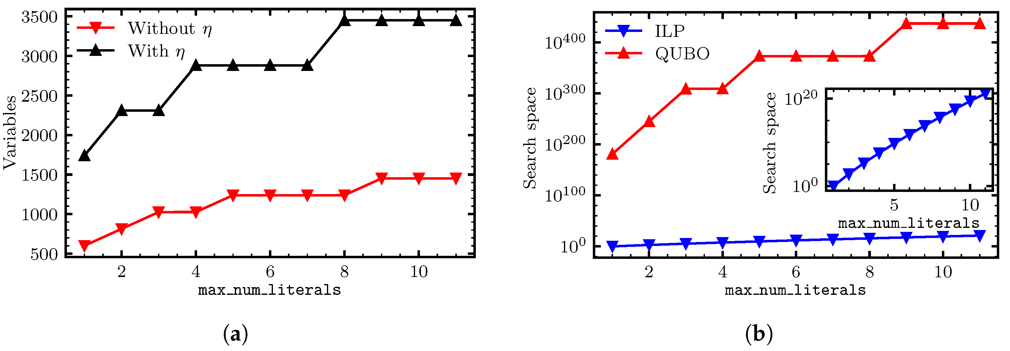
5.5. Reducing the Number of Variables

In this section, we describe a way of reducing the number of variables in the QUBO formulation by eliminating the error variables.

Recall that we introduced the misclassification indicator variables $\eta$ to soften the constraints. This inclusion made sense for the ILP formulation, in which the constraints would otherwise be applied as hard constraints. In QUBO formulations, the difference between soft and hard constraints is solely in the magnitude of the penalty coefficients. Therefore, we can, in principle, eliminate the error variables from the “imperfect” formulations and then add the constraints as soft constraints through construction, setting the penalty coefficients for those constraints to be relatively small.

For example, for the Or operator, we take Equation (20), delete the error variables from the objective function and constraints, and label those constraints as “soft”:

$$\begin{array}{cccc}\hfill & min\hfill & \hfill & \lambda (||\mathit{b}|{|}_0+||\tilde{\mathit{b}}|{|}_0)\hfill \\ \hfill & \mathrm{s}.\mathrm{t}.\hfill & \hfill & {\mathit{X}}_{\mathit{P}}(\mathit{b}-\tilde{\mathit{b}})+\left|\right|\tilde{\mathit{b}}{\left|\right|}_0\ge \mathbf{1}\left(\mathrm{Soft}\right)\hfill \\ \hfill & \hfill & & {\mathit{X}}_{\mathit{N}}(\mathit{b}-\tilde{\mathit{b}})+\left|\right|\tilde{\mathit{b}}{\left|\right|}_0=\mathbf{0}\left(\mathrm{Soft}\right)\hfill \\ \hfill & & \hfill & {\left|\right|\mathit{b}\left|\right|}_0+\left|\right|\tilde{\mathit{b}}{\left|\right|}_0\le m^{\prime }\hfill \\ \hfill & \hfill & & \mathit{b},\tilde{\mathit{b}}\in {\{0,1\}}^m.\hfill \end{array}$$

(22)

We then apply the recipe described in Section 5.4 to each constraint and add the class weights to find:

$$\begin{array}{cccc}\hfill & min\hfill & \hfill & \lambda (||\mathit{b}|{|}_0+||\tilde{\mathit{b}}|{|}_0)+\hfill \\ \hfill & \hfill & & w_P{L}_1{\left\{{\mathit{X}}_{\mathit{P}}(\mathit{b}-\tilde{\mathit{b}})+\left|\right|\tilde{\mathit{b}}{\left|\right|}_0-\mathbf{1}-\mathit{s}\right\}}^2+\hfill \\ \hfill & \hfill & & w_N{L}_1{\left\{{\mathit{X}}_{\mathit{N}}(\mathit{b}-\tilde{\mathit{b}})+\left|\right|\tilde{\mathit{b}}{\left|\right|}_0\right\}}^2+\hfill \\ \hfill & & \hfill & L_2{\left[{\left|\right|\mathit{b}\left|\right|}_0+\left|\right|\tilde{\mathit{b}}{\left|\right|}_0-m^{\prime }-t\right]}^2\hfill \\ \hfill & \mathrm{s}.\mathrm{t}.\hfill & \hfill & \mathit{b},\tilde{\mathit{b}}\in {\{0,1\}}^m,\hfill \end{array}$$

(23)

where we use the same curly bracket notation used in Equation (21), $\mathit{s}$ is a vector of the slack variables, t is a slack variable, and $L_1$ and $L_2$ are positive penalty coefficients. As before, the strength of the constraint imposing the maximum number of literals should be much larger than the strength of the soft constraints to ensure it is enforced, i.e., $L_2\gg L_1$.

The reduction in the problem size due to softening the constraints is generally significant (see

Table 2. Number of variables required for various QUBO and ILP formulations. “Operator” is the operator at the root of the depth-one rule, “with $\eta$” refers to the QUBO formulation in which misclassifications are allowed via additional error variables, “without $\eta$” refers to the QUBO formulation in which misclassifications are allowed by soft constraints. The numbers quoted are for the complete Breast Cancer dataset, which contains 63% negative labels, with max_num_literals $=4$.

Operator	with $\mathit{\eta }$	without $\mathit{\eta }$	ILP
Or	2879	1027	1169
And	2879	1317	1169
AtLeast	3097	1959	1170
AtMost	3097	1959	1170
Choose	3811	2673	1527

). For example, for the Or formulation, we save the addition of the $\eta$ variables, one per sample. However, the dominant savings are in the slack variables for the negative data rows because those constraints become equality constraints, thus avoiding the need for slack variables. In addition, there is a reduction in the range of the slack variables for the positive data rows, which can result in an additional reduction. The number of variables for each formulation is given by

$$\begin{array}{ccc}\hfill & \mathtt{\text{num}}\_\mathtt{\text{vars}}=2m+n+\lceil {log}_2(m^{\prime }+1)\rceil (n+1)\hfill & \left(\mathrm{Or}\mathrm{with}\eta \right)\hfill \\ \hfill & \mathtt{\text{num}}\_\mathtt{\text{vars}}=2m+\lceil {log}_2(m^{\prime }+1)\rceil +\lceil {log}_2\left(m^{\prime }\right)\rceil n_P\hfill & \left(\mathrm{Or}\mathrm{without}\eta \right).\hfill \end{array}$$

(24)

We hypothesize that the reduced problem size likely leads to a reduced time to solution (TTS). The TTS is commonly calculated as the product of the average time taken for a single start $\tau$ and the number of starts required to find an optimum with a certain confidence level, usually 99%, referred to as $R_{99}$, i.e., $\mathrm{TTS}=\tau R_{99}$ [13]. The reduction in the problem size should yield a shorter time per iteration, resulting in a smaller $\tau$. In addition, one might expect the problem difficulty to be reduced, resulting in a smaller $R_{99}$, but this is not guaranteed, as smaller problems are generally, but not always, easier.

For the results of the experiment comparing the two formulations (with/without $\eta$) for the Or and And operators, see Figure 11. We observe, anecdotally, that the “without $\eta$” formulation leads to a similar or better accuracy–complexity curve, and even when both formulations have similar performance, the runtime for the formulation without $\eta$ is much shorter (potentially by orders of magnitude). This is in line with the above theoretical arguments; however, we defer a detailed comparison of the TTS for the two formulations for future work.

Finally, it is worth noting that the elimination of error variables causes the solution space to be biased. The objective function in this case is a sum of squares of violations (residuals) of the sample constraints. Therefore, given two solutions that have the same score S (i.e., degenerate solutions), the solution with the lower sum of squares of violations is preferred. In some sense, one might argue that this bias is reasonable because the solution that is preferred is “wrong by less” than the solution with the larger sum of squares of violations.

5.6. Number of Variables and the Nature of the Search Space

When calculating the Pareto frontier, we aim to solve a series of optimization problems starting from a small complexity bound $m^{\prime }$ (i.e., max_num_literals) and gradually increasing it. For this reason, it is interesting to consider the dependence of the number of variables and the search space size on $m^{\prime }$. For simplicity, we limit this discussion to non-parameterized operators.

In Equation (24), we can see that for a fixed dataset of dimensions $n\times m$, the number of variables in the QUBO formulations increases in a step-wise fashion as $m^{\prime }$ increases (see Figure 12a). The search space size for each of the QUBO formulations is given by $2^{\mathtt{\text{num}}\_\mathtt{\text{vars}}}$, where num_vars is the number of variables in the respective formulation. The size of the search space for the ILP formulation, which is exactly equal to the feasible space, is much smaller and is given by

$$\mathtt{\text{num}}\_\mathtt{feasible}=\sum _{l=0}^{m^{\prime }}\left(\genfrac{}{}{0pt}{}{2m}{l}\right).$$

(25)

For a visual comparison of the sizes of the infeasible space (QUBO) and the feasible space (ILP), see Figure 12b. It is clear that the space searched by the QUBO formulations is far larger than the feasible space, handicapping the QUBO solver. For example, for $\mathtt{max}\_\mathtt{num}\_\mathtt{literals}\approx 10$, we find that the QUBO search space surpasses the ILP search space by more than 400 orders of magnitude. This motivates, in part, the usage of the QUBO solver as a subproblem solver, as described later in this paper, instead of for solving the whole problem. When solving smaller subproblems, the size gap between the feasible space and the infeasible space is relatively smaller and might be surmountable by a fast QUBO solver.

Furthermore, by inspecting the constraints, we can see that moving from a feasible solution to another feasible solution requires flipping more than a single bit. This means that the search space is composed of single feasible solutions, each surrounded by many infeasible solutions with higher objective function values, like islands in an ocean. This situation is typical for constrained QUBO problems. Under these conditions, we expect that a single bit-flip optimizer, such as single bit-flip simulated annealing, would be at a distinct disadvantage. In contrast, this situation should, in principle, be good for quantum optimization algorithms (including quantum annealing) because these barriers between the feasible solutions are narrow and, therefore, should be relatively easy to tunnel through [54].

6. Benchmarking Methodology and Results

In this section, we describe our research questions and the setup for our numerical experiments and we present and discuss our results.

6.1. Research Questions

We consider the following research questions (RQ) to demonstrate the effectiveness of our approach:

RQ1. 

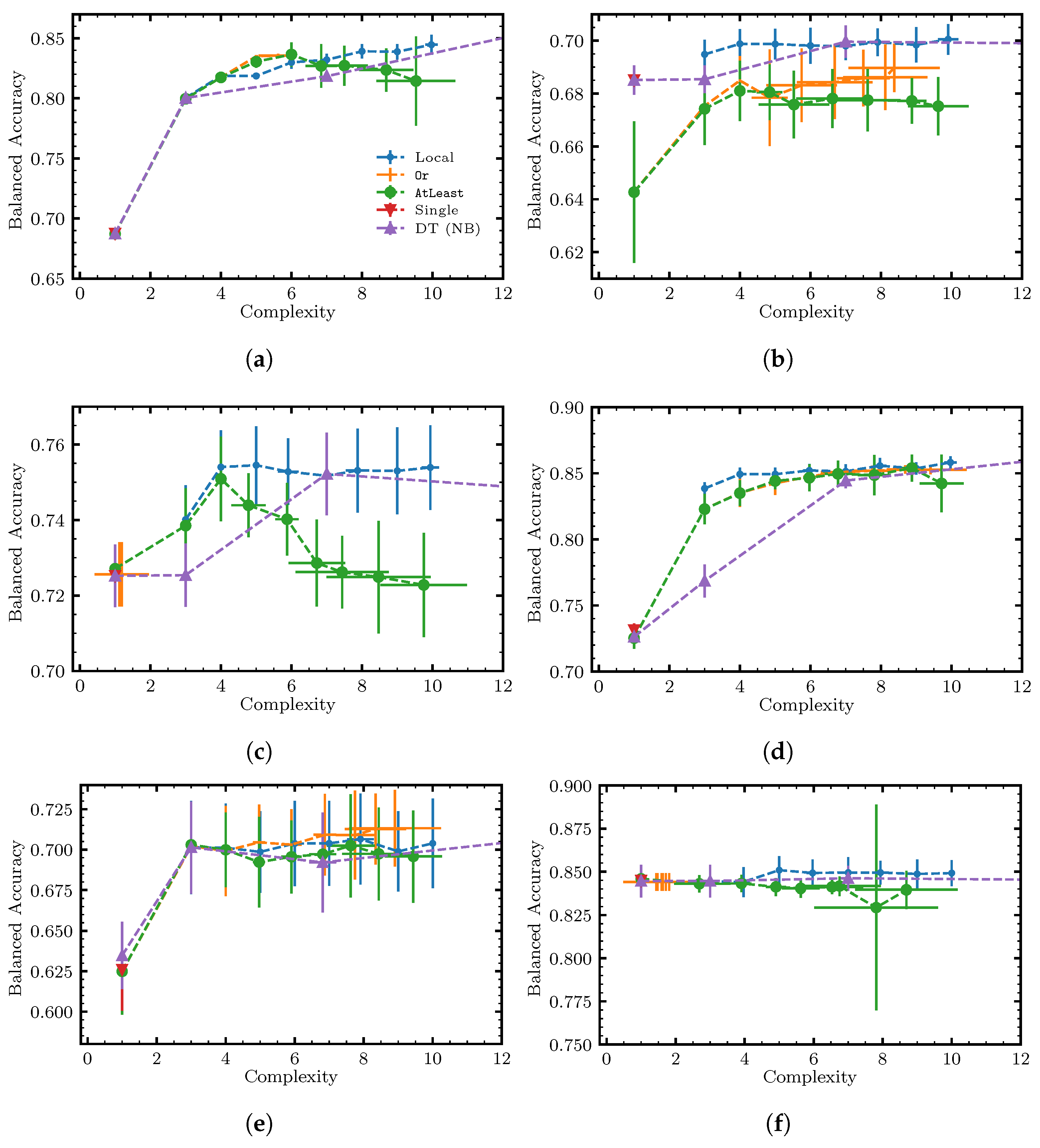
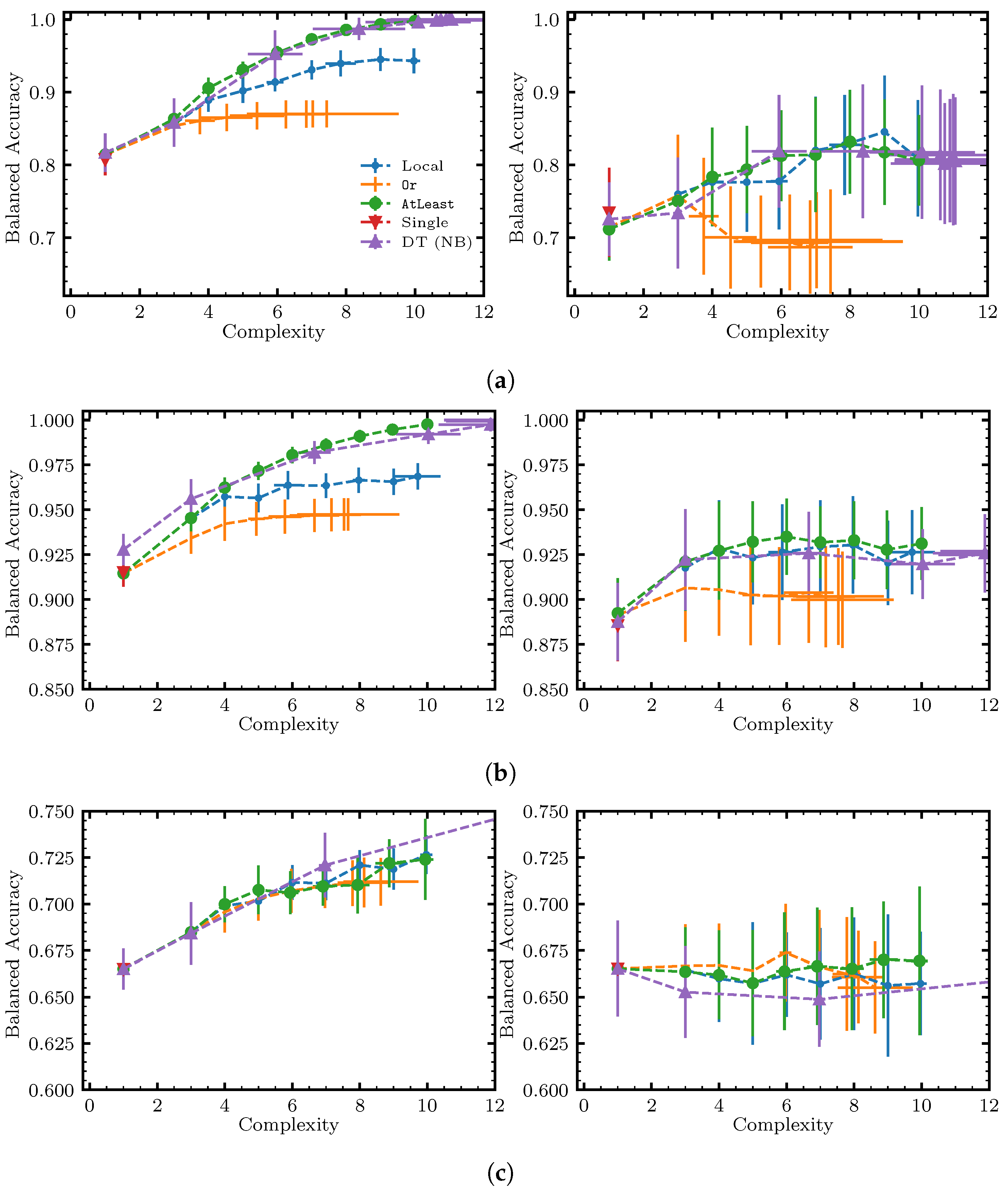
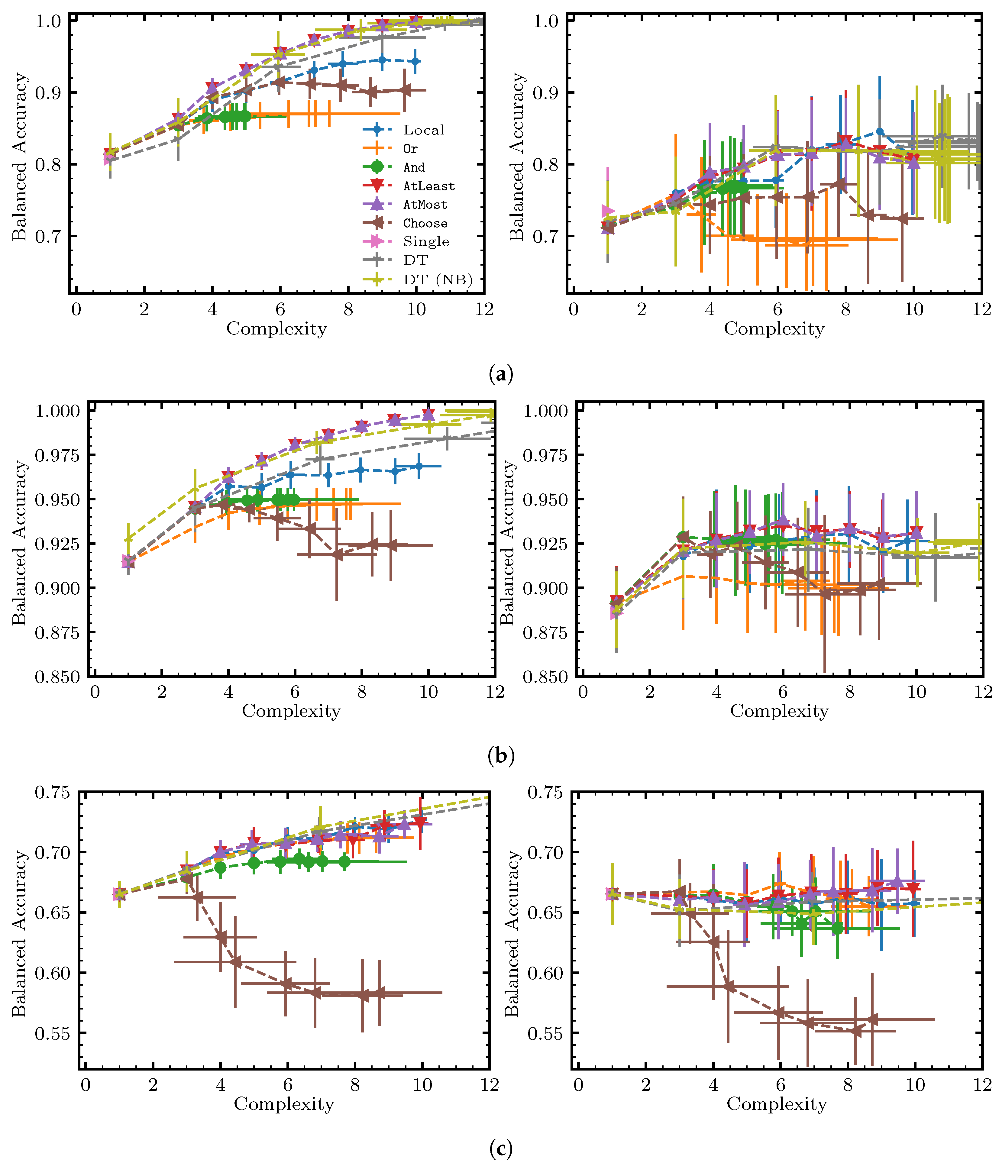
What is the performance of each solution approach with respect to the Pareto frontier, i.e., score vs. complexity?

RQ2. 

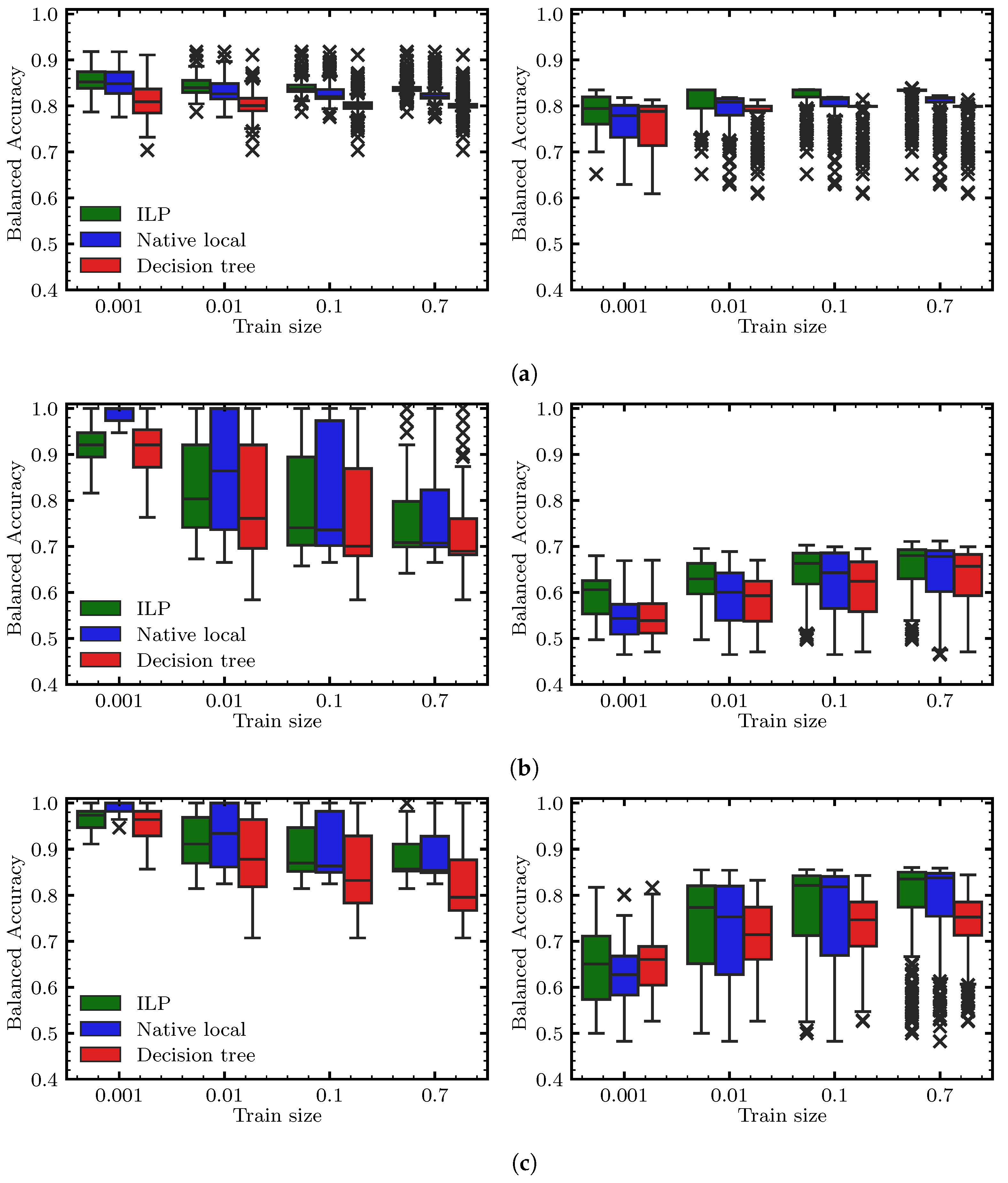
Does sampling help scale to large datasets?

RQ3. 

Are non-local moves advantageous vs. using just local moves, and under what conditions?

6.2. Benchmarking Methodology

Datasets—The binary classification datasets included in our experiments are shown in

Table 3. Datasets included in our experiments. “Rows” is the number of data samples with no missing values, “Features” is the number of features provided, “Binarized” is the number of features after binarization, “Majority” is the fraction of data rows belonging to the larger of the two classes, and “Ref.” is a reference for each dataset.

Name	Rows	Features	Binarized	Majority	Ref.
Airline Customer Satisfaction	129,487	22	119	0.55	[55]
Breast Cancer	569	30	300	0.63	[40]
Credit Card Default	30,000	23	185	0.78	[56]
Credit Risk	1000	20	92	0.70	[57]
Customer Churn	7043	19	67	0.73	[58]
Direct Marketing	41,188	20	124	0.89	[53]
Home Equity Default	3364	12	93	0.80	[59]
Online Shoppers’ Intentions	12,330	17	104	0.85	[60]
Parkinson’s	195	22	217	0.75	[61]

. We selected datasets with varied characteristics. In particular, the number of samples ranged from 195 (very small) to $\sim 1.3\times {10}^5$ (very large) and the number of binarized features ranged from 67 to 300.

Several datasets included in our study contained samples with missing data, which were removed prior to using the data. We removed 393 samples from the Airline Customer Satisfaction dataset, 11 samples from the Customer Churn dataset, and 2596 samples from the Home Equity Default dataset. The first two were negligible, but the latter comprised 44% of the data.

Binarization—To form Boolean rules, all input features must be binary. For this reason, we binarized any features that were not already binary. Features that were already binary did not require special treatment. Features that were categorical or numerical with few unique values were binarized using one-hot encoding. For features that are numerical with many unique values, many binarization methods are available, including splitting them into equal-count bins, equal-width bins, or bins that maximize the information gain [62]. We hypothesize that the choice of method of binarization can have a strong effect on downstream ML models, although we defer this to future work.

In this paper, binarization was carried out by binning the features followed by encoding the features using one-hot encoding. The binning was carried out by calculating num_bins quantiles for each feature. For each quantile, a single “up” bin was defined, extending from that quantile value to infinity. Because our classifiers all included the negated features, the corresponding “down” bins were already included by way of those negated features. In all experiments, we set num_bins $=10$.

Classifiers—We included several classifiers in our experiments. First, the baseline classifiers used were as follows:

• Most frequent—A naive classifier that always outputs the label that is most frequent in the training data. This classifier always gives exactly 0.5 for balanced accuracy. We excluded this classifier from the figures to reduce clutter and because we considered it a lower baseline. This classifier was easily outperformed by all the other classifiers.
• Single feature—A classifier that consists of a simple rule, containing only a single feature. The rule is determined in training by exhaustively checking all possible rules consisting of a single feature or a single negated feature.
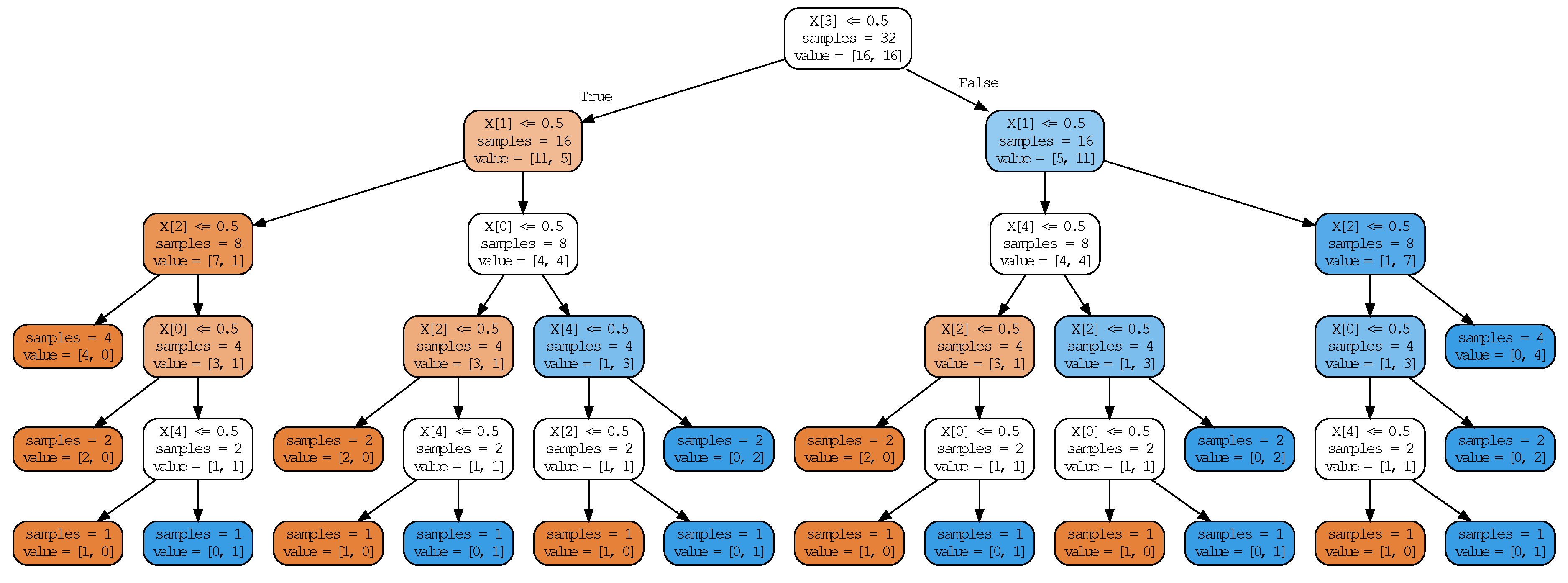
• Decision tree—A decision tree classifier, as implemented in scikit-learn [36], with class_weight = “balanced”. Note that decision trees are able to take non-binary inputs, so we also included the results obtained by training a decision tree on the raw data with no binarization. To control the complexity of the decision tree, we varied max_depth, which sets the maximum depth of the trained decision tree. The complexity is given by the number of split nodes (as described in Section 3.4).

The depth-one QUBO and ILP classifiers used were as follows:

• ILP rule—A classifier that solves the ILP formulations, as described in Section 5.1, Section 5.2 and Section 5.3 for a depth-one rule with a given operator at the root, utilizing FICO Xpress (version 9.0.1) with a timeout of one hour. To limit the size of the problems, a maximum of 3000 samples was used for each cross-validation split.
• QUBO rule—A classifier that solves the QUBO formulations, as described in Section 5.4 for a depth-one rule with a given operator at the root, utilizing simulated annealing, as implemented in dwave-neal with num_reads $=100$ and num_sweeps $=2000$. To limit the size of the problems, a maximum of 3000 samples was used for each cross-validation split. The results were generally worse than those of the ILP classifier (guaranteed not to be better in terms of score), so to reduce clutter, we did not include them below (but some QUBO results can be seen in Figure 11). A likely explanation for the underwhelming results is explained in Section 5.6—this is a single bit-flip optimizer, but going from a feasible solution to a feasible solution in our QUBO formulations requires flipping more than one variable at a time.

Finally, the native local solvers used were as follows:

• SA native local rule—The simulated annealing native local rule classifier, as described in Section 4.5, with $\mathtt{num}\_\mathtt{starts}=20$, and $\mathtt{num}\_\mathtt{iterations}=2000$. The temperatures follow a geometric schedule from 0.2 to ${10}^{-6}$.
• SA native non-local rule—The simulated annealing native local rule classifier with additional ILP-powered non-local moves, as described in Section 4.6. This classifier uses the same parameter values as the native local rule classifier and, in addition, the burn-in period consists of the first third of the steps, $\mathtt{patience}=10$, $\mathtt{max}\_\mathtt{samples}=100$, and the timeout for the ILP solver was set to one second.

Cross-validation—Each dataset was split into in-sample data and out-of-sample data using an 80/20 stratified split. The in-sample data were then shuffled and split 32 times (unless indicated otherwise in each experiment) into training/test data with a 70/30 stratified split. All benchmarking runs were performed on Amazon EC2, utilizing c5a.16xlarge instances with 64 vCPUs and 128 GiB of RAM. Cross-validation for each classifier and dataset was generally performed on 32 splits in parallel in separate processes on the same instance.

Hyperparameter optimization—Very minimal hyperparameter optimization was performed—it was assumed that the results could be improved through parameter tuning, which was not the focus of this work. In addition, it is possible that using advanced techniques such as column generation for solving ILPs would measurably improve the results. Note that $\lambda =0$ was used in all experiments to simplify the analysis.

6.3. Results and Discussion

Pareto frontier (RQ1)—On each dataset, for each classifier, we report the mean and standard deviation of the balanced accuracy and the complexity over those splits for the training/test portions of the data. Some classifiers were unparameterized, so we report a single point for each dataset (single-feature classifier and most frequent classifier). The decision tree classifier results were obtained by changing the max_depth parameter over a range of values. For the depth-one QUBO and ILP classifiers, the results were obtained by changing the max_num_literals parameter over a range of values. Finally, for the native local optimizers, the results were obtained by changing the max_complexity parameter over a range of values. The decision tree was also run on the raw data without a binarizer, which is indicated by the suffix “(NB)”.

For all datasets, except for the three smallest ones (up to 1000 samples), the training and test results are virtually indistinguishable. For this reason, we present the training and test results for the smaller datasets, but only the test results for the larger datasets. The similarity between the training and test results is likely due to the fact that our classifiers are (by design) highly regularized by virtue of binarization and their low complexity. Therefore, they do not seem to be able to overfit the data, as long as the data size is not very small.

Figure 13 shows the training and test results for the three smallest datasets, and Figure 14 shows the test results for the six larger datasets. Finally, some example rules found by the native local optimizer for each of the datasets are presented in

Table 4. Example rules obtained by the native local solver for each dataset. “Dataset” is the name of the dataset and “Rule” is the best rule found by the first of the cross-validation splits for the case max_complexity $=4$. The variable names in the rules are obtained from the original datasets. Negations of features are post-processed by reversing the relationship in the respective feature name (e.g., $\sim a=3\to a\ne 3$).

Dataset	Rule
Airline Customer Satisfaction	And(Inflight entertainment ≠ 5, Inflight entertainment ≠ 4, Seat comfort ≠ 0)
Breast Cancer	AtMost1(worst concave points ≤ 0.1533, worst radius ≤ 16.43, mean texture ≤ 15.3036)
Credit Card Default	Or(PAY_2 > 0, PAY_0 > 0, PAY_4 > 0)
Credit Risk	Choose1(checking_status = no checking, checking_status < 200, property_magnitude = real estate)
Customer Churn	AtMost1(tenure > 5, Contract ≠ Month-to-month, InternetService ≠ Fiber optic)
Direct Marketing	Or(duration > 393, nr.employed ≤ 5076.2, month = mar)
Home Equity Default	Or(DEBTINC > 41.6283, DELINQ ≠ 0.0, CLNO ≤ 11)
Online Shoppers’ Intentions	AtMost1(PageValues ≤ 5.5514, PageValues ≤ 0, BounceRates > 0.025)
Parkinson’s	AtMost1(spread1 > −6.3025, spread2 > 0.1995, Jitter:DDP > 0.0059)

.

The native local rule classifier was generally found to be competitive with the other classifiers, achieving similar scores to the decision tree, despite the decision tree involving a more flexible optimization procedure. The ILP classifiers were shallower but still achieved similar scores to the native local solver on most datasets. However, the ILP classifiers required significantly longer run times. This suggests that the additional depth did not always provide an advantage. However, for some of the datasets, such as Direct Marketing and Customer Churn, there was a slight advantage for the native local solver, and hence an apparent advantage to deeper rules. However, note that deeper rules could be considered less interpretable and less desirable for the XAI use case.

Of note, the single-feature rule classifier baseline outperformed or matched the other classifiers on the Credit Card Default, Credit Risk, and Online Shoppers’ Intentions datasets, suggesting that for those datasets, a more complex model than those included in this work is required to achieve higher scores. The best score achieved varied significantly across the datasets studied, suggesting that they featured a range of hardnesses.

For all datasets except Parkinson’s, the great majority of the decision tree classifier’s results had such a high complexity that they were outside of the plot. This is another example of the issue pointed out in Section 3.4—decision trees tend to yield high-complexity trees/rules, even for single-digit values of max_depth.

When comparing the different ILP operators, the results suggest that the parameterized operators AtMost and AtLeast offer an advantage over the unparameterized operators, which could be explained by their additional expressivity. We note that the performance of AtMost and AtLeast was largely identical, in line with the similarity of these operators. The results for the third parameterized operator, Choose, were poor for some of the datasets, likely due to the larger problem size in this formulation, resulting in the ILP solver timing out before finding a good solution. In fact, many of the other ILP runs timed out despite sampling down the larger datasets to 3,000 samples (for training), which suggests that trying to prove optimality for large datasets might not be scalable. Furthermore, as anticipated in Section 5.2, for some of the datasets, the results for the And operator were better than those for the Or operator (for example, on the Breast Cancer dataset).

Sampling (RQ2)—The main objective of this experiment was to assess whether large datasets can be tackled via sampling, i.e., by selecting a subsample of the data to be used for training the classifier (see Figure 15). This experiment was run only on the three largest datasets to allow for room to change the sample size.

We observed that the training score decreased with the training sample size until saturation, presumably because it is harder to fit a larger dataset. At the same time, the test score increased with the training sample size, presumably because the larger sample provides better representation and, therefore, the ability to generalize. The score distribution on the training and test sets generally narrowed with the increasing training sample size, presumably converging on the population’s score. We observed that the training and test scores were initially very different for small training sample sizes but converged to similar values for large training sample sizes. These results suggest that several thousand samples might be enough to reach a stable score for the ILP and native local solvers compared to deep learning techniques that often require far more data (for example, [63]). We also note that the sampling procedure is attractive due to its simplicity and it being classifier agnostic.

Native non-local solver (RQ3)—The main objective of this experiment was to assess whether the non-local moves provided an advantage and under what conditions. With this in mind, we varied both max_complexity and num_iterations, as shown in Figure 16.

In the training results, it is clear that the non-local moves result in a meaningful improvement (several percentage points in terms of balanced accuracy) on two out of the three datasets (and a marginal improvement on the third), but only at a higher complexity, suggesting that one can use the non-local moves to fit the data with a smaller number of iterations. If a solver is available that can solve the optimization problem to find non-local moves quickly, using such a solver might lead to faster training. At a lower complexity, there is not enough “room” for the non-local moves to operate, so they do not provide an advantage.

In the test results, the error bars are overlapping so it is not possible to make a strong statement. However, we note that the point estimates for the mean are slightly improved over the whole range of complexities for all three datasets.

Note that the very short timeout for the ILP solver to find each non-local move likely curtailed the solver’s ability to find good moves. In addition, ILP solvers typically have many parameters that control their operation, which were not adjusted in this case. It is likely that asking the solver to focus on quickly finding good solutions would improve the results. We leave this direction for future research.

7. Conclusions and Outlook

We have introduced the concept of expressive Boolean formulas, motivated by the relative rigidity and lower expressivity of other techniques such as decision trees and CNF rules. We then proposed a class of interpretable ML classification models based on these formulas. These models were trained via native local optimization, with a flexible choice of operators. In our work, native local optimization was carried out via a simulated annealing algorithm, but other choices are possible.

It is also possible to make larger, non-local moves. In our work, non-local moves were proposed by solving an optimization problem that can be formulated as an ILP or a QUBO problem. As such, we foresee an opportunity to gain potential speedups by using hardware accelerators, including future quantum computers. We studied a depth-one formulation for non-local moves, which could be extended to specific depth-two forms. The formulations we introduced for finding non-local moves are also usable as standalone classifiers, in which the Boolean rule forming the basis for the classifier is very shallow (depth-one).

A limitation of our work is the requirement that the input data be binary. For non-binary data, this introduces a dependence on the binarization method. For some data types, binarization may not make sense or may result in a significant loss of information (such as for images). As presented here, an additional limitation is that the labels must be a single binary output. In practice, there are methods of extending the applicability of a binary classifier to multi-class and multi-output classification. This is outside the scope of this work but is included in the accompanying Python library (see below).

Finally, we highlight possible extensions of this research that extend beyond our present work, such as the following:

• Datasets—The classifiers proposed here could be applied to other datasets, for example, in finance, healthcare, and life sciences.
• Operators—The definition of expressive Boolean formulas is (by design) flexible, as well as the operation of the corresponding classifiers. In particular, it is possible to remove some of the operators used in this study or introduce new operators such as AllEqual or Xor depending on the particular problem at hand.
• Use cases—The idea of representing data using a series of operators could be applied to other use cases, such as circuit synthesis [64].
• Binarization—The dependence on the binarization scheme could be studied. Early experiments we ran with another binarization scheme (based on equal-count bins) showed worse results. This raises the possibility that another binarization scheme may improve the presented results.
• Implementation—Our implementation for the native local solver was written in Python (see http://github.com/fidelity/boolxai for the open-sourced version of the native local solver, which will be available soon) and was not heavily optimized. We expect that our implementation of the native local solver could be significantly sped up, for example, by implementing it in a lower-level language or by judicious use of memoization.

At present, quantum computers are resource-limited and noisy, making solving optimality difficult/expensive, even for small optimization problems. However, solving the XAI problem to optimality is not strictly required in most practical scenarios, thus potentially lowering the requirements on noise for quantum devices. The QUBO and ILP formulations we have presented could be solved, in principle, by a number of quantum algorithms, such as the Quantum Approximate Optimization Algorithm (QAOA) [42]. Follow-up work may investigate the performance and resource requirements of quantum algorithms on these problems. Furthermore, there is potential to apply quantum computers to other aspects of XAI.

References

- Burkart, N.; Huber, M.F. A survey on the explainability of supervised machine learning. J. Artif. Intell. Res. 2021, 70, 245–317. [Google Scholar] [CrossRef]
- Slack, D.; Hilgard, S.; Jia, E.; Singh, S.; Lakkaraju, H. Fooling LIME and SHAP: Adversarial attacks on post hoc explanation methods. In Proceedings of the AAAI/ACM Conference on AI, Ethics, and Society, New York, NY, USA, 7–8 February 2020; pp. 180–186. [Google Scholar]
- Lakkaraju, H.; Arsov, N.; Bastani, O. Robust and stable black box explanations. arXiv 2020, arXiv:2011.06169. [Google Scholar]
- Letham, B.; Rudin, C.; McCormick, T.H.; Madigan, D. Interpretable classifiers using rules and Bayesian analysis: Building a better stroke prediction model. Ann. Appl. Stat. 2015, 9, 1350–1371. [Google Scholar] [CrossRef]
- Wang, F.; Rudin, C. Falling rule lists. arXiv 2015, arXiv:1411.5899. [Google Scholar]
- Lakkaraju, H.; Bach, S.H.; Leskovec, J. Interpretable decision sets: A joint framework for description and prediction. In Proceedings of the 22nd ACM SIGKDD International Conference on Knowledge Discovery and Data Mining, San Francisco, CA, USA, 13–17 August 2016; pp. 1675–1684. [Google Scholar]
- Ustun, B.; Rudin, C. Supersparse linear integer models for optimized medical scoring systems. Mach. Learn. 2016, 102, 349–391. [Google Scholar] [CrossRef]
- Angelino, E.; Larus-Stone, N.; Alabi, D.; Seltzer, M.; Rudin, C. Learning certifiably optimal rule lists. In Proceedings of the 23rd ACM SIGKDD International Conference on Knowledge Discovery and Data Mining, Halifax, NS, Canada, 13–17 August 2017; pp. 35–44. [Google Scholar]
- Zahedinejad, E.; Zaribafiyan, A. Combinatorial optimization on gate model quantum computers: A survey. arXiv 2017, arXiv:1708.05294. [Google Scholar]
- Sanders, Y.R.; Berry, D.W.; Costa, P.C.S.; Tessler, L.W.; Wiebe, N.; Gidney, C.; Neven, H.; Babbush, R. Compilation of fault-tolerant quantum heuristics for combinatorial optimization. PRX Quantum 2020, 1, 020312. [Google Scholar] [CrossRef]
- Reuther, A.; Michaleas, P.; Jones, M.; Gadepally, V.; Samsi, S.; Kepner, J. Survey and benchmarking of machine learning accelerators. In Proceedings of the 2019 IEEE High Performance Extreme Computing Conference (HPEC), Waltham, MA, USA, 24–26 September 2019; pp. 1–9. [Google Scholar]
- Bavikadi, S.; Dhavlle, A.; Ganguly, A.; Haridass, A.; Hendy, H.; Merkel, C.; Reddi, V.J.; Sutradhar, P.R.; Joseph, A.; Dinakarrao, S.M.P. A survey on machine learning accelerators and evolutionary hardware platforms. IEEE Design Test 2022, 39, 91–116. [Google Scholar] [CrossRef]
- Aramon, M.; Rosenberg, G.; Valiante, E.; Miyazawa, T.; Tamura, H.; Katzgraber, H.G. Physics-inspired optimization for quadratic unconstrained problems using a digital annealer. Front. Phys. 2019, 7, 48. [Google Scholar] [CrossRef]
- Mohseni, N.; McMahon, P.L.; Byrnes, T. Ising machines as hardware solvers of combinatorial optimization problems. Nat. Rev. Phys. 2020, 4, 363–379. [Google Scholar] [CrossRef]
- Valiante, E.; Hernandez, M.; Barzegar, A.; Katzgraber, H.G. Computational overhead of locality reduction in binary optimization problems. Comput. Phys. Commun. 2021, 269, 108102. [Google Scholar] [CrossRef]
- Fedus, W.; Zoph, B.; Shazeer, N. Switch transformers: Scaling to trillion parameter models with simple and efficient sparsity. J. Mach. Learn. Res. 2022, 23, 1–39. [Google Scholar]
- Ribeiro, M.T.; Singh, S.; Guestrin, C. Why should I trust you? Explaining the predictions of any classifier. In Proceedings of the 22nd ACM SIGKDD International Conference on Knowledge Discovery and Data Mining, San Francisco, CA, USA, 13–17 August 2016; pp. 1135–1144. [Google Scholar]
- Lundberg, S.M.; Lee, S.-I. A unified approach to interpreting model predictions. arXiv 2017, arXiv:1705.07874. [Google Scholar]
- Lakkaraju, H.; Kamar, E.; Caruana, R.; Leskovec, J. Faithful and customizable explanations of black box models. In Proceedings of the 2019 AAAI/ACM Conference on AI, Ethics, and Society, Honolulu, HI, USA, 27–28 January 2019; pp. 131–138. [Google Scholar]
- Craven, M.; Shavlik, J. Extracting tree-structured representations of trained networks. Adv. Neural Inf. Process. Syst. 1995, 8, 24–30. [Google Scholar]
- Bastani, O.; Kim, C.; Bastani, H. Interpreting blackbox models via model extraction. arXiv 2017, arXiv:1705.08504. [Google Scholar]
- Malioutov, D.; Meel, K.S. MLIC: A MaxSAT-based framework for learning interpretable classification rules. In Proceedings of the International Conference on Principles and Practice of Constraint Programming, Lille, France, 27–31 August 2018; pp. 312–327. [Google Scholar]
- Ghosh, B.; Meel, K.S. IMLI: An incremental framework for MaxSAT-based learning of interpretable classification rules. In Proceedings of the 2019 AAAI/ACM Conference on AI, Ethics, and Society, Honolulu, HI, USA, 27–28 January 2019; pp. 203–210. [Google Scholar]
- Su, G.; Wei, D.; Varshney, K.R.; Malioutov, D.M. Interpretable two-level Boolean rule learning for classification. arXiv 2015, arXiv:1511.07361. [Google Scholar]
- Wang, T.; Rudin, C. Learning optimized Or’s of And’s. arXiv 2015, arXiv:1511.02210. [Google Scholar]
- Lawless, C.; Dash, S.; Gunluk, O.; Wei, D. Interpretable and fair boolean rule sets via column generation. arXiv 2021, arXiv:2111.08466. [Google Scholar]
- Malioutov, D.M.; Varshney, K.R.; Emad, A.; Dash, S. Learning interpretable classification rules with Boolean compressed sensing. In Transparent Data Mining for Big and Small Data; Springer: Berlin/Heidelberg, Germany, 2017; pp. 95–121. [Google Scholar]
- Rudin, C. Stop explaining black box machine learning models for high stakes decisions and use interpretable models instead. Nat. Mach. Intell. 2019, 1, 206–215. [Google Scholar] [CrossRef]
- Batcher, K.E. Sorting networks and their applications. In Proceedings of the Spring Joint Computer Conference, Atlantic City, NJ, USA, 30 April–2 May 1968; pp. 307–314. [Google Scholar]
- Asín, R.; Nieuwenhuis, R.; Oliveras, A.; Rodríguez-Carbonell, E. Cardinality networks and their applications. In Proceedings of the International Conference on Theory and Applications of Satisfiability Testing, Swansea, UK, 30 June–3 July 2009; pp. 167–180. [Google Scholar]
- Bailleux, O.; Boufkhad, Y. Efficient CNF encoding of Boolean cardinality constraints. In Proceedings of the International Conference on Principles and Practice of Constraint Programming, Kinsale, Ireland, 29 September–3 October 2003; pp. 108–122. [Google Scholar]
- Ogawa, T.; Liu, Y.; Ryuzo Hasegawa, R.; Koshimura, M.; Fujita, H. Modulo based CNF encoding of cardinality constraints and its application to MaxSAT solvers. In Proceedings of the 2013 IEEE 25th International Conference on Tools with Artificial Intelligence, Herndon, VA, USA, 4–6 November 2013; pp. 9–17. [Google Scholar]
- Morgado, A.; Ignatiev, A.; Marques-Silva, J. MSCG: Robust core-guided MaxSAT solving. J. Satisf. Boolean Model. Comput. 2014, 9, 129–134. [Google Scholar] [CrossRef]
- Sinz, C. Towards an optimal CNF encoding of Boolean cardinality constraints. In International Conference on Principles and Practice of Constraint Programming; Springer: Berlin/Heidelberg, Germany, 2005; pp. 827–831. [Google Scholar]
- Ignatiev, A.; Morgado, A.; Marques-Silva, J. PySAT: A Python toolkit for prototyping with SAT oracles. In SAT; Springer: Berlin/Heidelberg, Germany, 2018; pp. 428–437. [Google Scholar]
- Pedregosa, F.; Varoquaux, G.; Gramfort, A.; Michel, V.; Thirion, B.; Grisel, O.; Blondel, M.; Prettenhofer, P.; Weiss, R.; Dubourg, V.; et al. Scikit-learn: Machine learning in Python. J. Mach. Learn. Res. 2021, 12, 2825–2830. [Google Scholar]
- Hoos, H.H.; Stützle, T. Stochastic Local Search: Foundations and Applications; Elsevier: Amsterdam, The Netherlands, 2004. [Google Scholar]
- Pisinger, D.; Ropke, S. Large neighborhood search. In Handbook of Metaheuristics; Springer: Berlin/Heidelberg, Germany, 2019; pp. 99–127. [Google Scholar]
- Kirkpatrick, S.; Gelatt, C.D., Jr.; Vecchi, M.P. Optimization by simulated annealing. Science 1983, 220, 671–680. [Google Scholar] [CrossRef]
- Wolberg, W.H.; Street, W.N.; Mangasarian, O.L. Breast Cancer Wisconsin (Diagnostic) Data Set. UCI Machine Learning Repository. 1992. Available online: https://archive.ics.uci.edu/ml/datasets/breast+cancer (accessed on 1 November 2022).
- Durr, D.; Hoyer, P. A quantum algorithm for finding the minimum. arXiv 1996, arXiv:quant-ph/9607014. [Google Scholar]
- Farhi, E.; Goldstone, J.; Gutmann, S. A quantum approximate optimization algorithm. arXiv 2014, arXiv:1411.4028. [Google Scholar]
- Khosravi, F.; Scherer, A.; Ronagh, P. Mixed-integer programming using a Bosonic quantum computer. arXiv 2021, arXiv:2112.13917. [Google Scholar]
- Montanaro, A. Quantum speedup of branch-and-bound algorithms. Phys. Rev. Res. 2020, 2, 013056. [Google Scholar] [CrossRef]
- Bisschop, J. AIMMS modeling guide-integer programming tricks. In Pinedo, Michael. Scheduling: Theory, Algorithms, and Systems; AIMMS BV: Haarlem, The Netherlands, 2016. [Google Scholar]
- Hauke, P.; Katzgraber, H.G.; Lechner, W.; Nishimori, H.; Oliver, W.D. Perspectives of quantum annealing: Methods and implementations. Rep. Prog. Phys. 2020, 83, 054401. [Google Scholar] [CrossRef] [PubMed]
- Temme, K.; Osborne, T.J.; Vollbrecht, K.G.; Poulin, D.; Verstraete, F. Quantum Metropolis sampling. Nature 2011, 471, 87–90. [Google Scholar] [CrossRef]
- Baritompa, W.P.; Bulger, D.W.; Wood, G.R. Grover’s quantum algorithm applied to global optimization. SIAM J. Optim. 2005, 15, 1170–1184. [Google Scholar] [CrossRef]
- Tilly, J.; Chen, H.; Cao, S.; Picozzi, D.; Setia, K.; Li, Y.; Grant, E.; Wossnig, L.; Rungger, I.; Booth, G.H.; et al. The variational quantum eigensolver: A review of methods and best practices. Phys. Rep. 2022, 986, 1–128. [Google Scholar] [CrossRef]
- Glover, F.; Kochenberger, G.; Hennig, R.; Du, Y. Quantum bridge analytics I: A tutorial on formulating and using QUBO models. Ann. Oper. Res. 2022, 314, 141–183. [Google Scholar] [CrossRef]
- Yarkoni, S.; Raponi, E.; Bäck, T.; Schmitt, S. Quantum annealing for industry applications: Introduction and review. arXiv 2022, arXiv:2112.07491. [Google Scholar] [CrossRef]
- Error Sources for Problem Representation. 2023. Available online: https://docs.dwavesys.com/docs/latest/c_qpu_ice.html (accessed on 15 March 2023).
- Moro, S.; Cortez, P.; Rita, P. A data-driven approach to predict the success of bank telemarketing. Decis. Support Syst. 2014, 62, 22–31. [Google Scholar] [CrossRef]
- Farhi, E.; Goldstone, J.; Gutmann, S. Quantum adiabatic evolution algorithms versus simulated annealing. arXiv 2002, arXiv:quant-ph/0201031. [Google Scholar]
- Kaggle. Airline Customer Satisfaction. Kaggle. 2023. Available online: https://www.kaggle.com/datasets/sjleshrac/airlines-customer-satisfaction (accessed on 1 November 2022).
- Yeh, I.C.; Lien, C.-H. The comparisons of data mining techniques for the predictive accuracy of probability of default of credit card clients. Expert Syst. Appl. 2009, 36, 2473–2480. [Google Scholar] [CrossRef]
- Dua, D.; Graff, C. UCI Machine Learning Repository. 2017. Available online: http://archive.ics.uci.edu/ml (accessed on 1 November 2022).
- Kaggle. Telco Customer Churn. Kaggle. 2023. Available online: https://www.kaggle.com/datasets/blastchar/telco-customer-churn (accessed on 1 November 2022).
- Kaggle. Home Equity, Kaggle. 2023. Available online: https://www.kaggle.com/datasets/ajay1735/hmeq-data (accessed on 1 November 2022).
- Sakar, C.O.; Polat, S.O.; Katircioglu, M.; Kastro, Y. Real-time prediction of online shoppers’ purchasing intention using multilayer perceptron and LSTM recurrent neural networks. Neural Comput. Appl. 2019, 31, 6893–6908. [Google Scholar] [CrossRef]
- Little, M.; Mcsharry, P.; Roberts, S.; Costello, D.; Moroz, I. Exploiting nonlinear recurrence and fractal scaling properties for voice disorder detection. Biomed. Eng. Online 2007, 26, 23. [Google Scholar]
- Fayyad, U. Multi-interval discretization of continuous-valued attributes for classification learning. In Proceedings of the Thirteenth International Joint Conference on Artificial Intelligence (II), Chambery, France, 28 August–3 September 1993; Volume 2, pp. 1022–1027. [Google Scholar]
- Van der Ploeg, T.; Austin, P.C.; Steyerberg, E.W. Modern modelling techniques are data hungry: A simulation study for predicting dichotomous endpoints. BMC Med. Res. Methodol. 2014, 14, 1–13. [Google Scholar] [CrossRef]
- De Micheli, G. Synthesis and Optimization of Digital Circuits; McGraw-Hill Higher Education: Irvine, CA, USA, 1994. [Google Scholar]