
Transforming Simulated Data into Experimental Data Using Deep Learning for Vibration-Based Structural Health Monitoring


Abstract
:1. Introduction
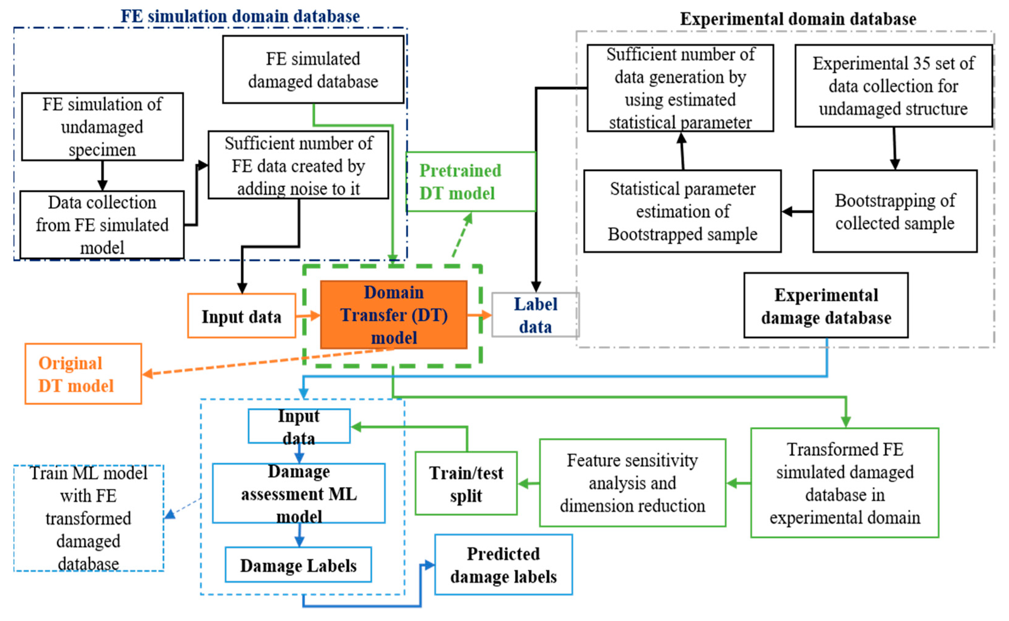
2. Methodology
Related Works
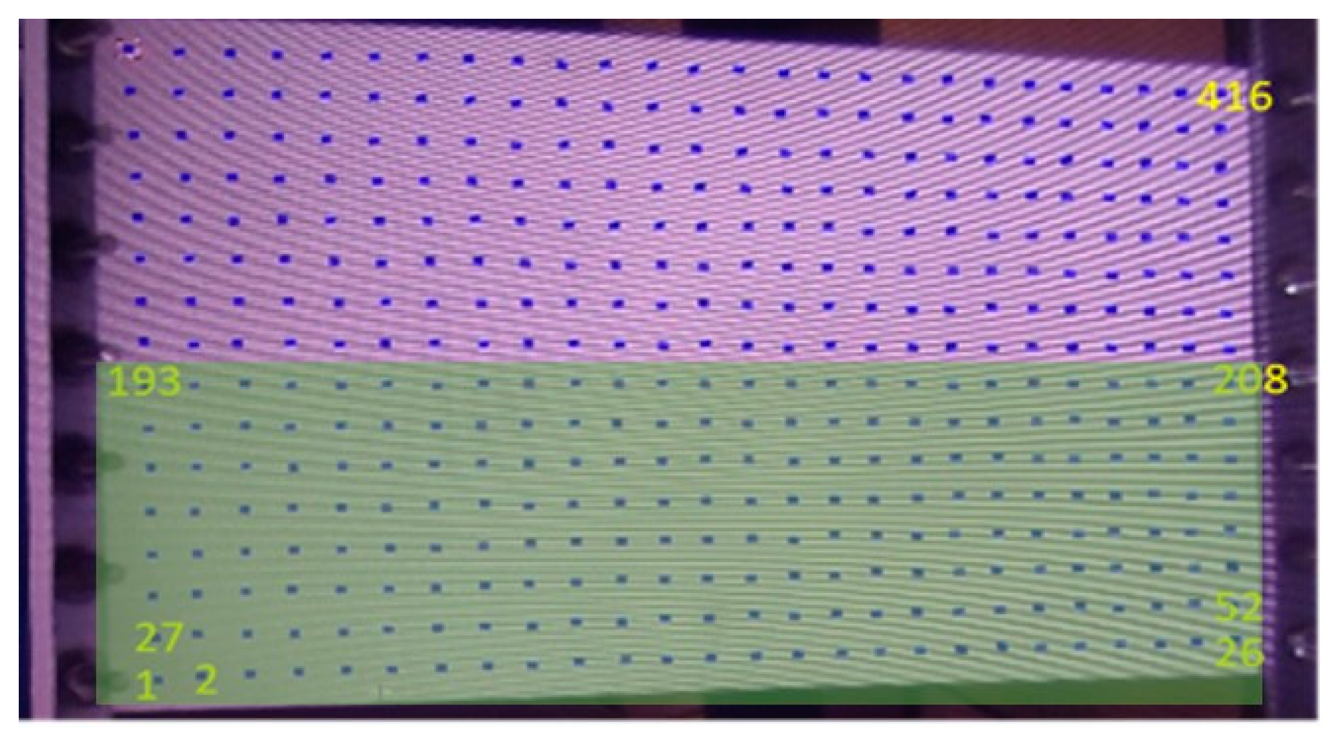
3. Experimental Setup and Specimen Detail
3.1. Test Specimen
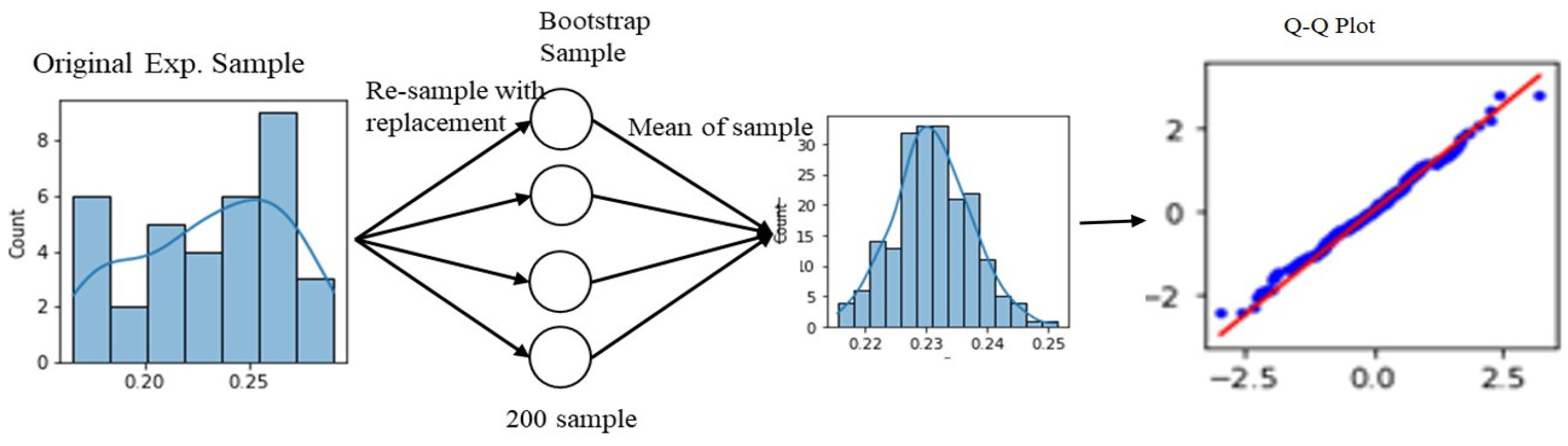
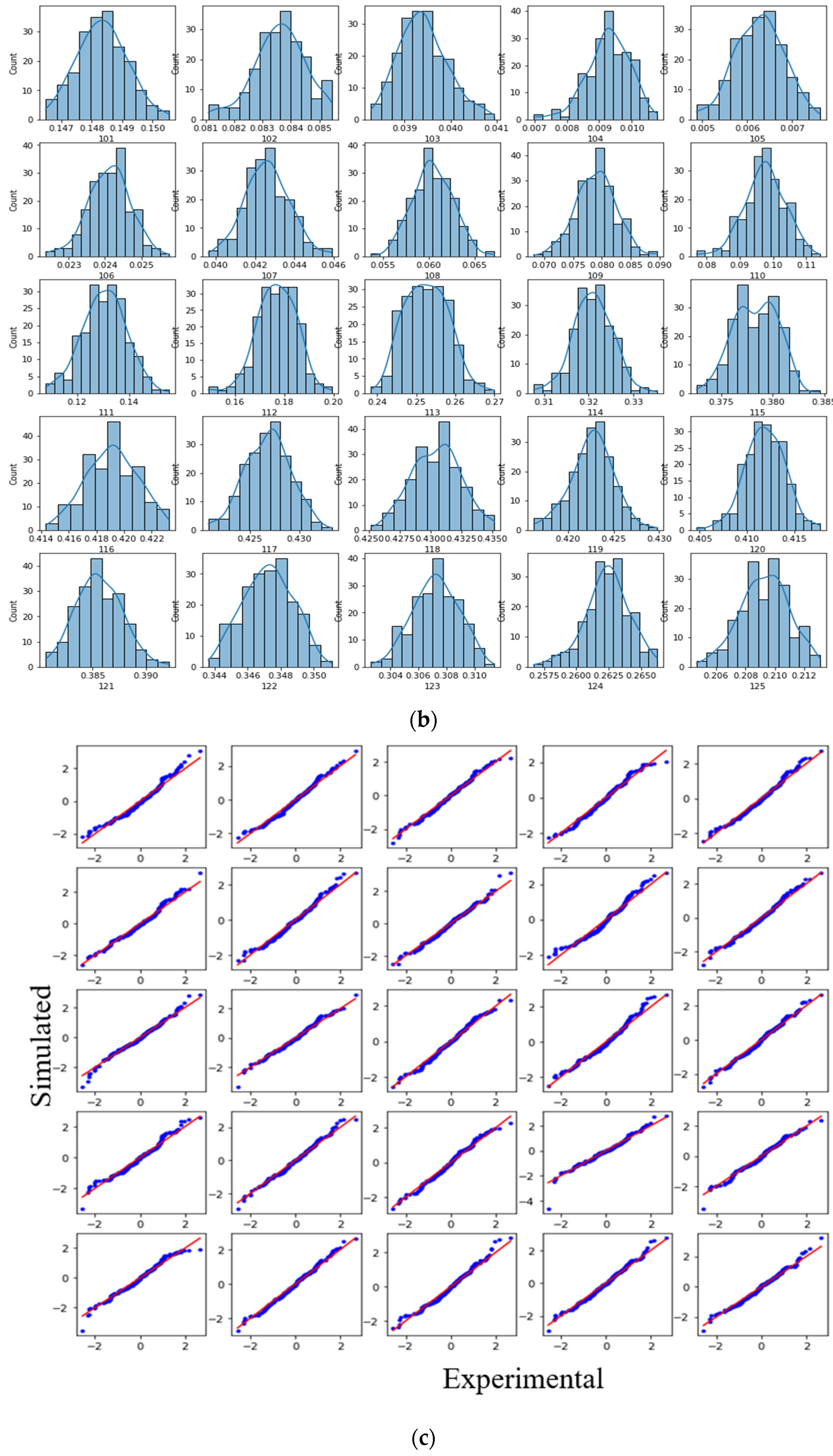
3.2. Experimental Variability Reduction
4. Numerical Modeling of Stiffened Panel
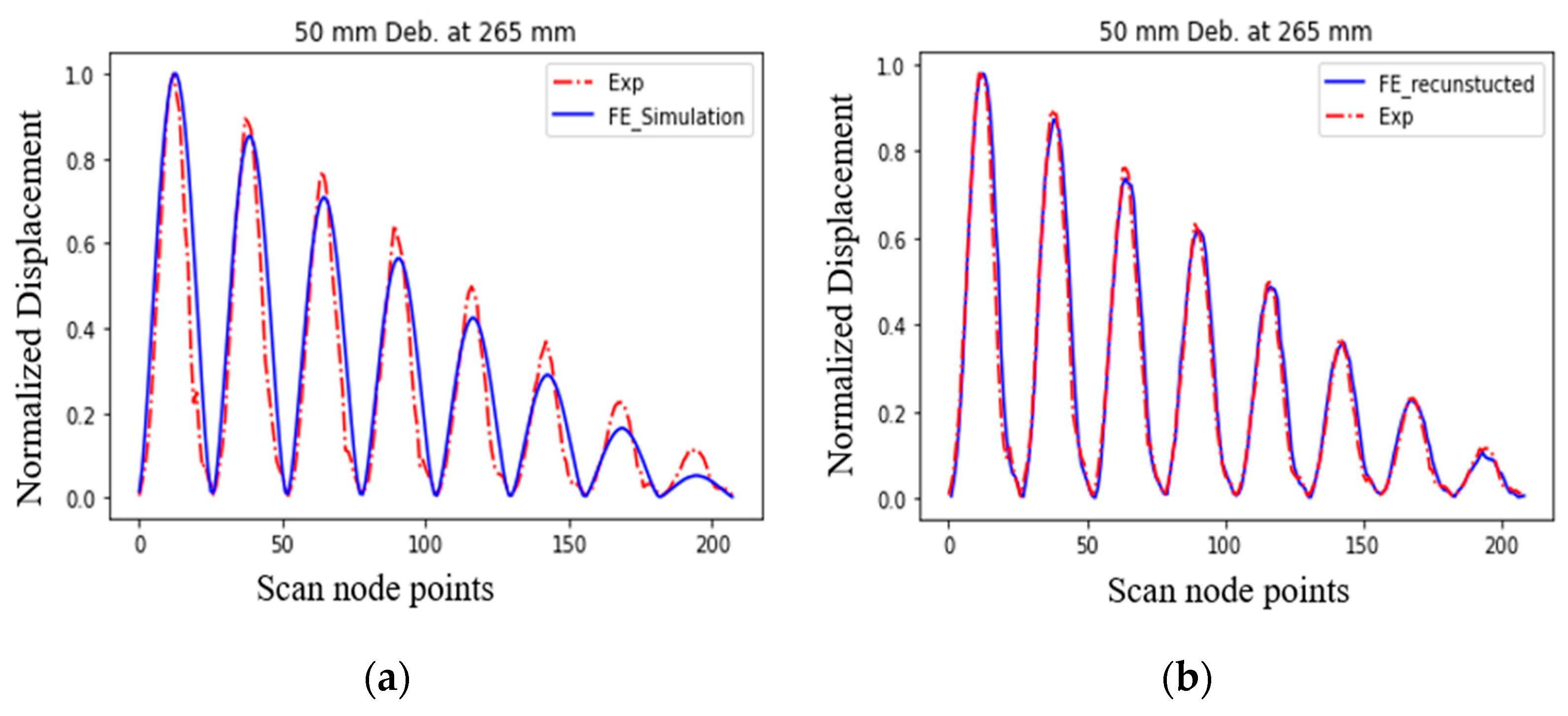
Numerical Model Verification with Experiment
5. Methodology Implementation
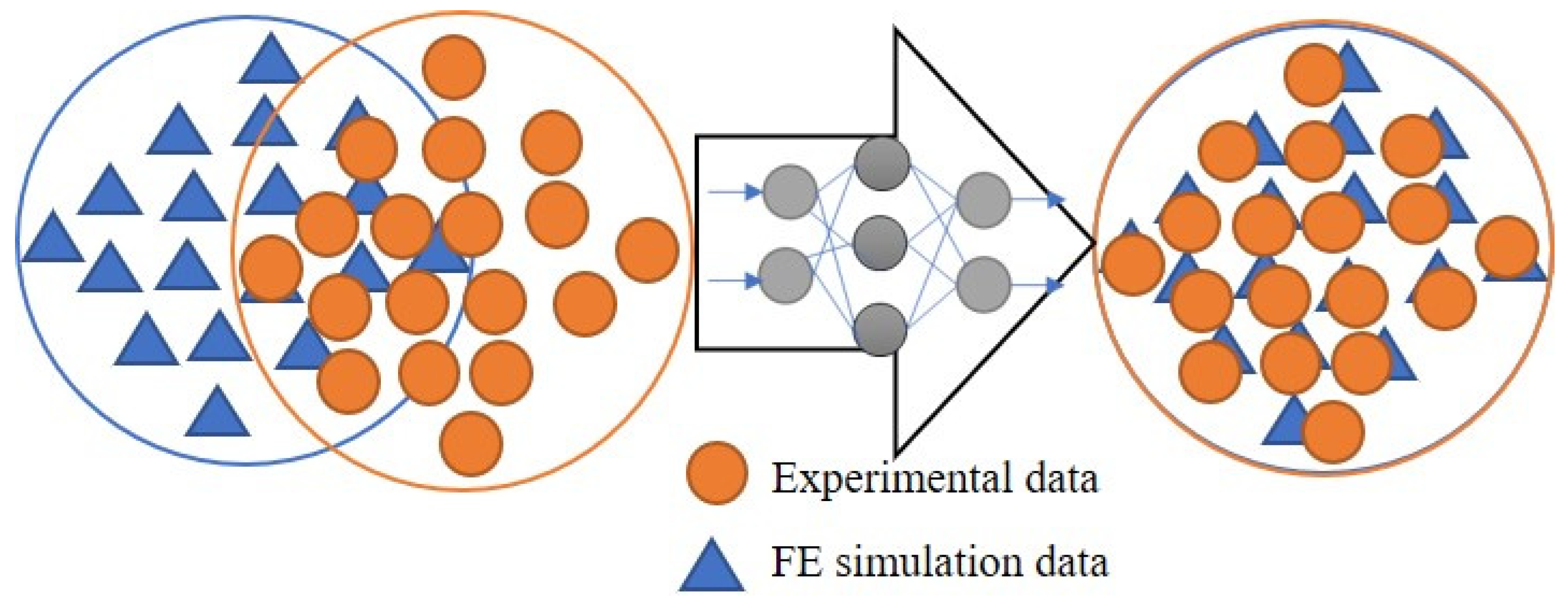
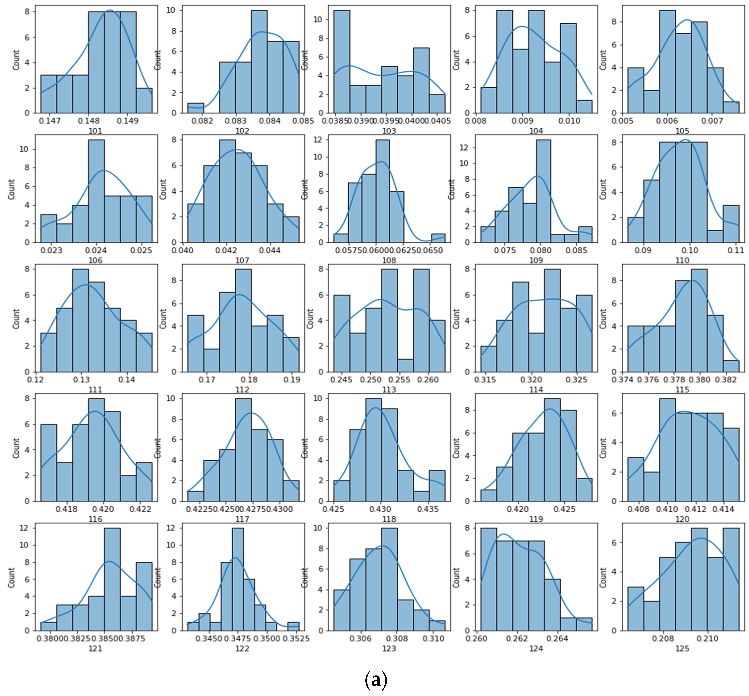
5.1. Data Preparation for Domain Transformation
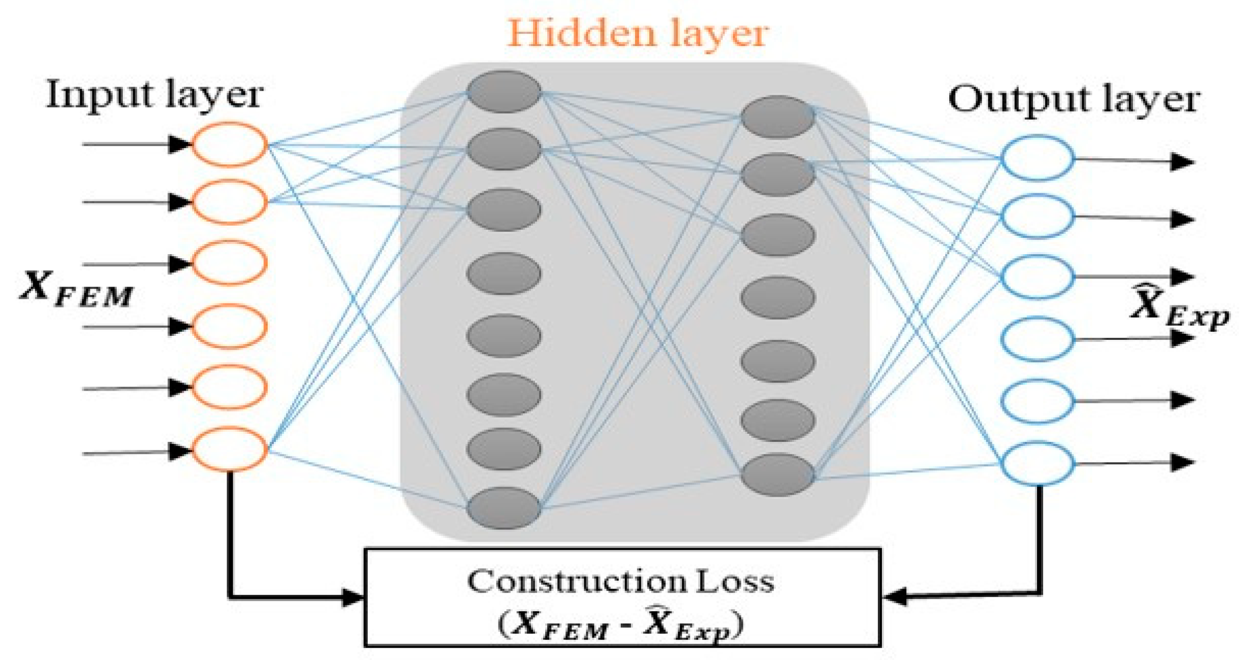
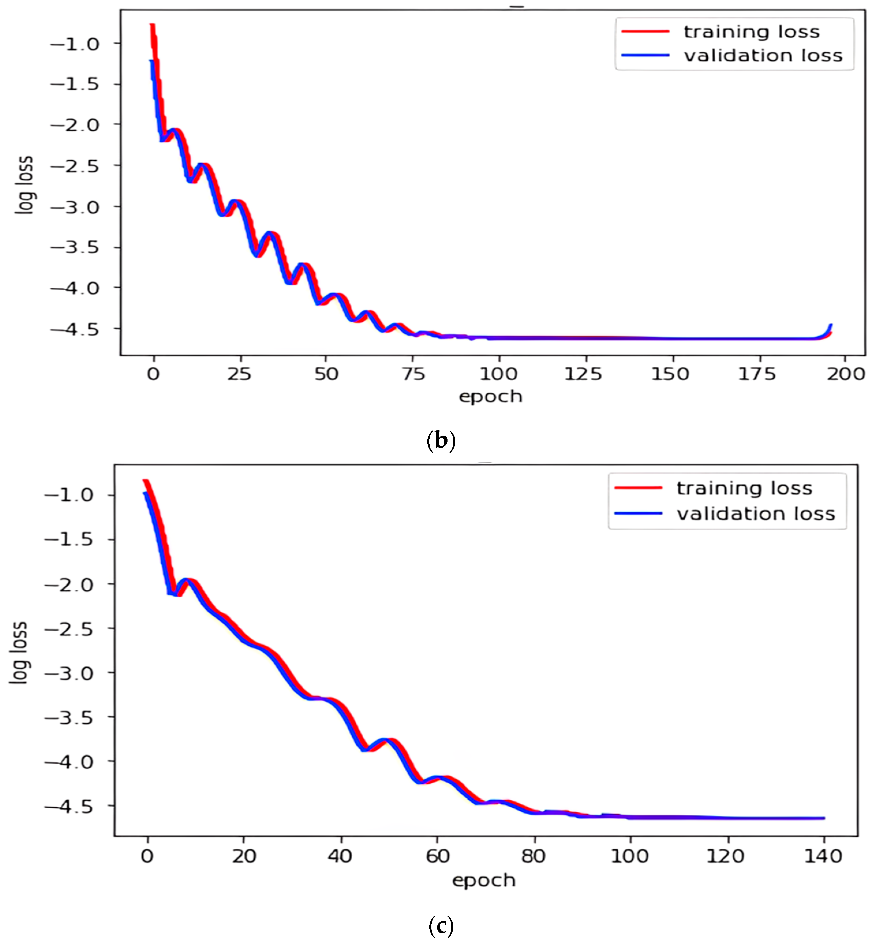
5.2. Domain Transformation Models
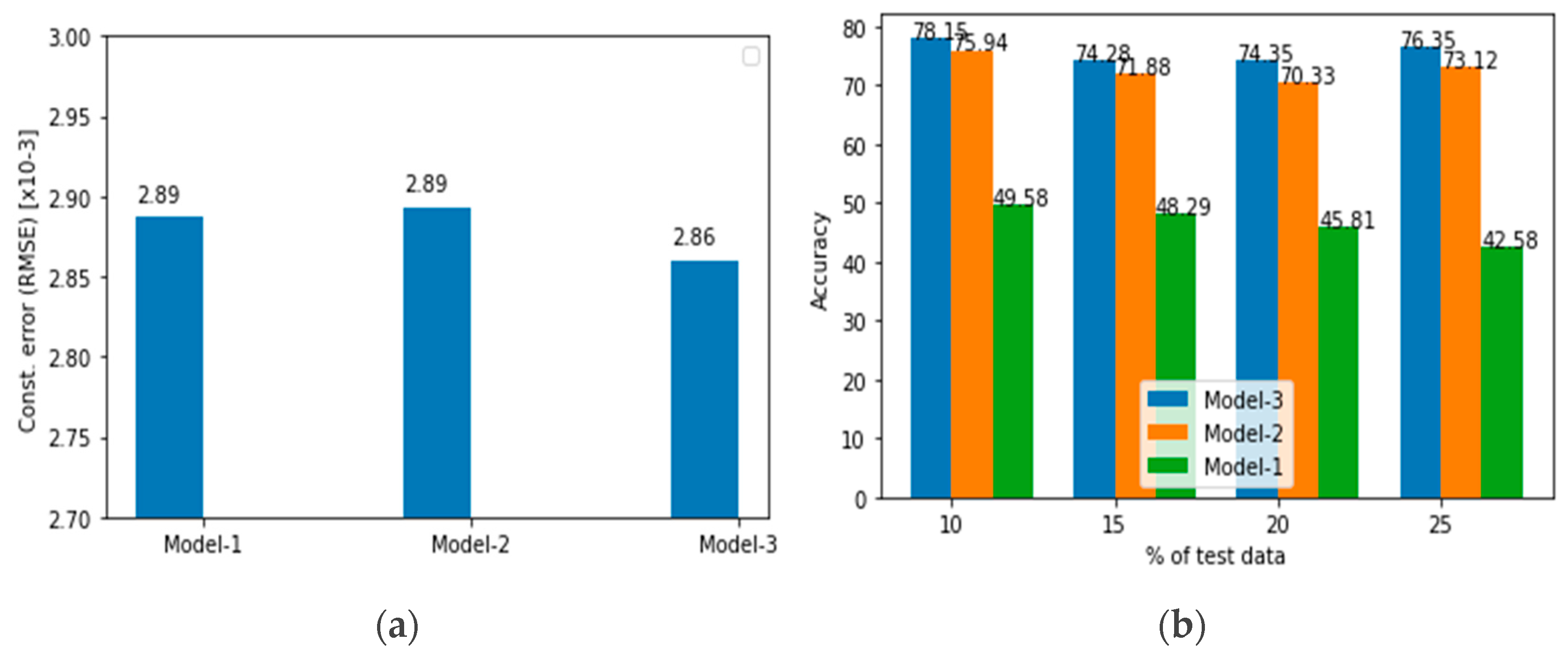
5.3. Comparison of DT Models
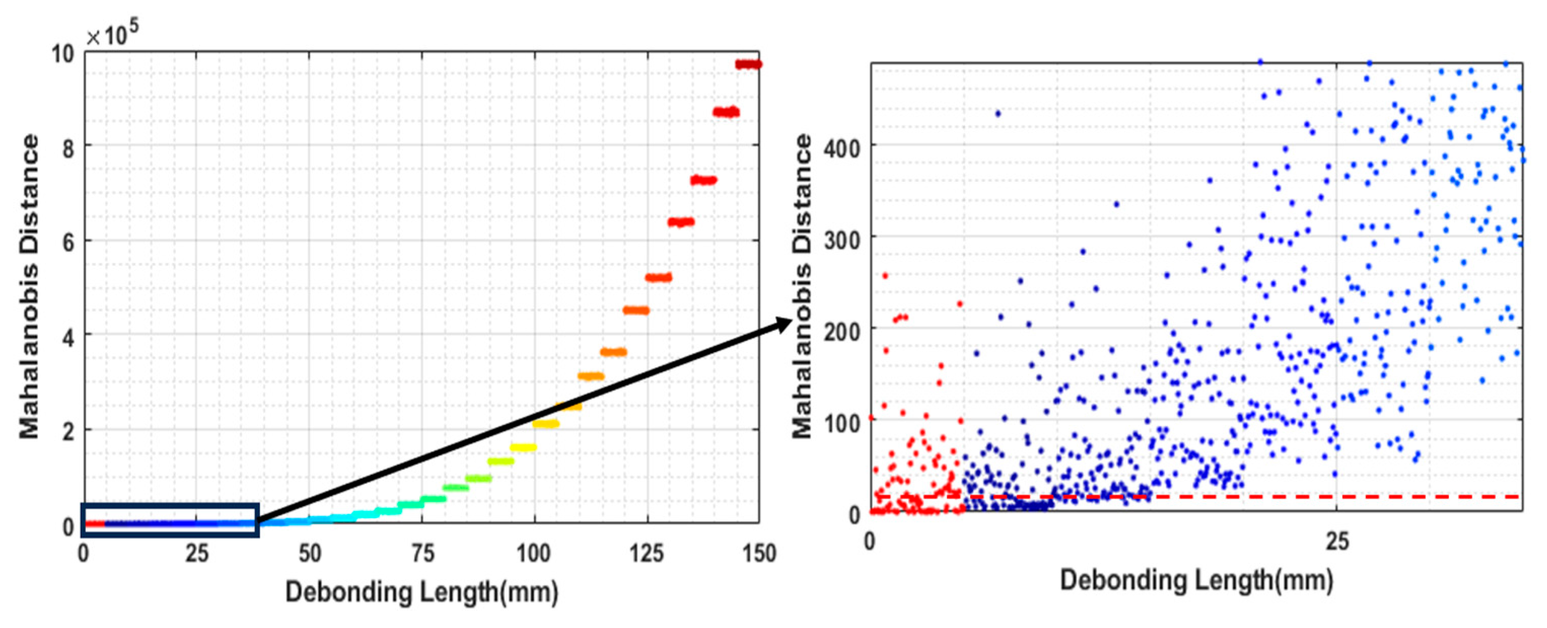
5.4. Damage Assessment
5.4.1. Feature Sensitivity Analysis
5.4.2. Feature Dimension Reduction
5.4.3. Dataset for Damaged Assessment
5.4.4. Performance Evaluation of ML Models in Damage Assessment
5.4.5. Results with FE-Transformed Data
5.4.6. Results with Experimental Data
6. Conclusions and Future Work
Author Contributions
Funding
Institutional Review Board Statement
Informed Consent Statement
Data Availability Statement
Acknowledgments
Conflicts of Interest
Appendix A

| Model-1 | |
|---|---|
| Layer (Type) | Output Shape |
| Input | (208) |
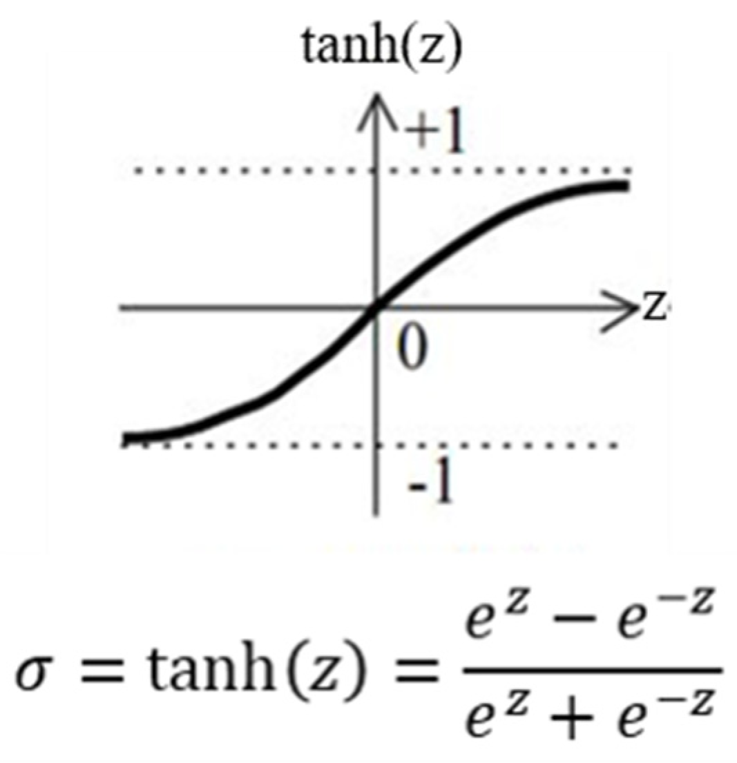
| Linear-1 (Tanh) | (1024) |
| Linear-2 (Tanh) | (512) |
| Output | (208) |
| Total parameters | 845,520 |
| Model-2 | |
| Layer (Type) | Output Shape |
| Input | (208) |
| Conv1D-1 (Tanh) (BN) | (16, 103) |
| Conv1D-2 (Tanh) (BN) | (32, 50) |
| Conv1D-3 (Tanh) (BN) | (64, 24) |
| Conv1D-4 (Tanh) (BN) | (128, 11) |
| Linear-1 (Tanh) | (1024) |
| Linear-2 (Tanh) | (512) |
| Output | (208) |
| Total parameters | 2,118,112 |
| Model-3 | |
| Layer (type) | Output Shape |
| Input | (208) |
| Conv1D-1 (Tanh) (BN) | (16, 103) |
| Conv1D-2 (Tanh) (BN) | (32, 50) |
| Conv1D-3 (Tanh) (BN) | (64, 24) |
| Conv1D-4 (Tanh) (BN) | (128, 11) |
| Linear-1 (Tanh) | (1024) |
| Linear-2 (Tanh) | (1408) |
| TransConv1D-1 (Tanh) (BN) | (64, 24) |
| TransConv1D-2 (Tanh) (BN) | (32, 50) |
| TransConv1D-3 (Tanh) (BN) | (16, 102) |
| Output | (208) |
| Total parameters | 2,905,641 |
References
- Farrar, C.R.; Worden, K.; Wiley, J. Structural Health Monitoring: A Machine Learning Perspective; John Wiley and Sons: Hoboken, NJ, USA, 2012. [Google Scholar]
- Figueiredo, E.; Park, G.; Farrar, C.R.; Worden, K.; Figueiras, J. Machine learning algorithms for damage detection under operational and environmental variability. Struct. Health Monit. 2010, 10, 559–572. [Google Scholar] [CrossRef]
- Yang, Z.; Yang, H.; Tian, T.; Deng, D.; Hu, M.; Ma, J.; Gao, D.; Zhang, J.; Ma, S.; Yang, L.; et al. A review on guided-ultrasonic-wave-based structural health monitoring: From fundamental theory to machine learning techniques. Ultrasonics 2023, 133, 107014. [Google Scholar] [CrossRef] [PubMed]
- Gordan, M.; Sabbagh-Yazdi, S.-R.; Ismail, Z.; Ghaedi, K.; Carroll, P.; McCrum, D.; Samali, B. State-of-the-art review on advancements of data mining in structural health monitoring. Measurement 2022, 193, 110939. [Google Scholar] [CrossRef]
- Toh, G.; Park, J. Review of Vibration-Based Structural Health Monitoring Using Deep Learning. Appl. Sci. 2020, 10, 1680. [Google Scholar] [CrossRef]
- Azimi, M.; Eslamlou, A.D.; Pekcan, G. Data-Driven Structural Health Monitoring and Damage Detection through Deep Learning: State-of-the-Art Review. Sensors 2020, 20, 2778. [Google Scholar] [CrossRef] [PubMed]
- Jayawickrema, U.; Herath, H.; Hettiarachchi, N.; Sooriyaarachchi, H.; Epaarachchi, J. Fibre-optic sensor and deep learning-based structural health monitoring systems for civil structures: A review. Measurement 2022, 199, 111543. [Google Scholar] [CrossRef]
- Civera, M.; Surace, C. Non-Destructive Techniques for the Condition and Structural Health Monitoring of Wind Turbines: A Literature Review of the Last 20 Years. Sensors 2022, 22, 1627. [Google Scholar] [CrossRef]
- Zhang, C.; Mousavi, A.A.; Masri, S.F.; Gholipour, G.; Yan, K.; Li, X. Vibration feature extraction using signal processing techniques for structural health monitoring: A review. Mech. Syst. Signal Process. 2022, 177, 109175. [Google Scholar] [CrossRef]
- Eltouny, K.; Gomaa, M.; Liang, X. Unsupervised Learning Methods for Data-Driven Vibration-Based Structural Health Monitoring: A Review. Sensors 2023, 23, 3290. [Google Scholar] [CrossRef]
- Kudva, J.N.; Munir, N.; Tan, P.W. Damage detection in smart structures using neural networks and finite-element analyses. Smart Mater. Struct. 1992, 1, 108–112. [Google Scholar] [CrossRef]
- Worden, K.; Ball, A.D.; Tomlinson, G.R. Fault location in a framework structure using neural networks. Smart Mater. Struct. 1993, 2, 189–200. [Google Scholar] [CrossRef]
- Sbarufatti, C.; Manes, A.; Giglio, M. Performance optimization of a diagnostic system based upon a simulated strain field for fatigue damage characterization. Mech. Syst. Signal Process. 2013, 40, 667–690. [Google Scholar] [CrossRef]
- Sbarufatti, C.; Manson, G.; Worden, K. A numerically-enhanced machine learning approach to damage diagnosis using a Lamb wave sensing network. J. Sound Vib. 2014, 333, 4499–4525. [Google Scholar] [CrossRef]
- Su, Z.; Ye, L. Lamb wave-based quantitative identification of delamination in CF/EP composite structures using artificial neural algorithm. Compos. Struct. 2004, 66, 627–637. [Google Scholar] [CrossRef]
- Su, Z.; Ye, L. Lamb Wave Propagation-based Damage Identification for Quasi-isotropic CF/EP Composite Laminates Using Artificial Neural Algorithm: Part I—Methodology and Database Development. J. Intell. Mater. Syst. Struct. 2005, 16, 97–111. [Google Scholar] [CrossRef]
- Gardner, P.; Liu, X.; Worden, K. On the application of domain adaptation in structural health monitoring. Mech. Syst. Signal Process. 2020, 138, 106550. [Google Scholar] [CrossRef]
- Zhang, S.; Li, C.M.; Yang, J.; Ye, W. Effective combination of modeling and experimental data with deep metric learning for guided wave-based damage localization in plates. Mech. Syst. Signal Process. 2022, 172, 108979. [Google Scholar] [CrossRef]
- De Fenza, A.; Sorrentino, A.; Vitiello, P. Application of Artificial Neural Networks and Probability Ellipse methods for damage detection using Lamb waves. Compos. Struct. 2015, 133, 390–403. [Google Scholar] [CrossRef]
- Kumar, A.; Guha, A.; Banerjee, S. A Methodology for Diagnosis of Damage by Machine Learning Algorithm on Experimental Data. In Lecture Notes in Civil Engineering; Rizzo, P., Milazzo, A., Eds.; Springer: Cham, Switzerland, 2021; Volume 128, pp. 91–105. [Google Scholar] [CrossRef]
- Barthorpe, R.; Manson, G.; Worden, K. On multi-site damage identification using single-site training data. J. Sound Vib. 2017, 409, 43–64. [Google Scholar] [CrossRef]
- Bao, N.; Zhang, T.; Huang, R.; Biswal, S.; Su, J.; Wang, Y. A Deep Transfer Learning Network for Structural Condition Identification with Limited Real-World Training Data. Struct. Control Health Monit. 2023, 2023, 8899806. [Google Scholar] [CrossRef]
- Efron, B.; Tibshirani, R. The Bootstrap Method for Assessing Statistical Accuracy. Behaviormetrika 1985, 12, 1–35. [Google Scholar] [CrossRef]
- Semaan, R. The uncertainty of the experimentally-measured momentum coefficient. Exp. Fluids 2020, 61, 248. [Google Scholar] [CrossRef]
- Carroll, A.; Sanders-O’connor, E.; Forrest, K.; Fynes-Clinton, S.; York, A.; Ziaei, M.; Flynn, L.; Bower, J.M.; Reutens, D. Improving Emotion Regulation, Well-being, and Neuro-cognitive Functioning in Teachers: A Matched Controlled Study Comparing the Mindfulness-Based Stress Reduction and Health Enhancement Programs. Mindfulness 2021, 13, 123–144. [Google Scholar] [CrossRef]
- Mahmoud, O.; Dudbridge, F.; Smith, G.D.; Munafo, M.; Tilling, K. A robust method for collider bias correction in conditional genome-wide association studies. Nat. Commun. 2022, 13, 619. [Google Scholar] [CrossRef]
- Renault, L.; McWilliams, J.C.; Kessouri, F.; Jousse, A.; Frenzel, H.; Chen, R.; Deutsch, C. Evaluation of high-resolution atmospheric and oceanic simulations of the California Current System. Prog. Oceanogr. 2021, 195, 102564. [Google Scholar] [CrossRef]
- Ince, T.; Kiranyaz, S.; Eren, L.; Askar, M.; Gabbouj, M. Real-Time Motor Fault Detection by 1-D Convolutional Neural Networks. IEEE Trans. Ind. Electron. 2016, 63, 7067–7075. [Google Scholar] [CrossRef]
- Zan, T.; Wang, H.; Wang, M.; Liu, Z.; Gao, X. Application of Multi-Dimension Input Convolutional Neural Network in Fault Diagnosis of Rolling Bearings. Appl. Sci. 2019, 9, 2690. [Google Scholar] [CrossRef]
- Abdeljaber, O.; Avci, O.; Kiranyaz, S.; Gabbouj, M.; Inman, D.J. Real-time vibration-based structural damage detection using one-dimensional convolutional neural networks. J. Sound Vib. 2017, 388, 154–170. [Google Scholar] [CrossRef]
- Goodfellow, I.; Bengio, Y.; Courville, A. Deep Learning; MIT Press: Cambridge, MA, USA, 2016. [Google Scholar]
- Ioffe, S.; Szegedy, C. Batch normalization: Accelerating deep network training by reducing internal covariate shift. In Proceedings of the 2nd International Conference on Machine Learning (ICML 2015), Lille, France, 6–11 July 2015; Volume 1, pp. 448–456. [Google Scholar]
- Bishop, C.M. Neural Networks for Pattern Recognition; Oxford University Press: Oxford, UK, 1995. [Google Scholar]
- Worden, K.; Manson, G.; Fieller, N. Damage detection using outlier analysis. J. Sound Vib. 2000, 229, 647–667. [Google Scholar] [CrossRef]
- Cortes, C.; Vapnik, V. Support-vector networks. Mach. Learn. 1995, 20, 273–297. [Google Scholar] [CrossRef]
- Breiman, L. Random forests. Mach. Learn. 2001, 45, 5–32. [Google Scholar] [CrossRef]
- Cover, T.; Hart, P. Nearest neighbor pattern classification. IEEE Trans. Inf. Theory 1967, 13, 21–27. [Google Scholar] [CrossRef]
- Wolpert, D.H. Stacked generalization. Neural Netw. 1992, 5, 241–259. [Google Scholar] [CrossRef]
- Aldave, R.; Dussault, J.P. Systematic Ensemble Learning for Regression. arXiv 2014, arXiv:1403.7267. [Google Scholar] [CrossRef]
- Cao, C.; Wang, Z. IMCStacking: Cost-sensitive stacking learning with feature inverse mapping for imbalanced problems. Knowledge-Based Syst. 2018, 150, 27–37. [Google Scholar] [CrossRef]
- Kumar, A.; Guha, A.; Banerjee, S. Improving Prediction Accuracy for Debonding Quantification in Stiffened Plate by Meta-Learning Model. In Proceedings of the International Conference on Big Data, Machine Learning and Their Applications, Silchar, India, 19–20 December 2021; pp. 51–63. [Google Scholar] [CrossRef]
- Zhai, B.; Chen, J. Development of a stacked ensemble model for forecasting and analyzing daily average PM2.5 concentrations in Beijing, China. Sci. Total Environ. 2018, 635, 644–658. [Google Scholar] [CrossRef]
- Ozay, M.; Yarman-Vural, F.T. Hierarchical distance learning by stacking nearest neighbor classifiers. Inf. Fusion 2016, 29, 14–31. [Google Scholar] [CrossRef]
- Carrington, A.M.; Manuel, D.G.; Fieguth, P.W.; Ramsay, T.; Osmani, V.; Wernly, B.; Bennett, C.; Hawken, S.; Magwood, O.; Sheikh, Y.; et al. Deep ROC Analysis and AUC as Balanced Average Accuracy, for Improved Classifier Selection, Audit and Explanation. IEEE Trans. Pattern Anal. Mach. Intell. 2022, 45, 329–341. [Google Scholar] [CrossRef]
- Carrington, A.M.; Fieguth, P.W.; Qazi, H.; Holzinger, A.; Chen, H.H.; Mayr, F.; Manuel, D.G. A new concordant partial AUC and partial c statistic for imbalanced data in the evaluation of machine learning algorithms. BMC Med. Inform. Decis. Mak. 2020, 20, 4. [Google Scholar] [CrossRef]


| Authors | Method | Approach | Structure | Damage Type | Exp. Data Quantity |
|---|---|---|---|---|---|
| Sbarufatti et al., 2013 [13] | Scaling factor | Strain field | Helicopter fuselage | Fatigue damage | Less exp. data |
| Sbarufatti et al., 2013 [14] | Numerically-enhanced ML approach | Guided wave | Plate | Discontinuity | Less exp. data |
| Barthorpe and Worden 2017 [21] | Generating exp. data from one specimen | Vibration | Wing panel of airplane | Discontinuity | High exp. Data |
| Gardner and Worden 2019 [17] | Domain adaptation | Vibration | MDOF spring-mass body | Stiffness variation | Less exp. Data |
| Zhang et al., 2022 [18] | Effective combination of FE and exp. data | Guided wave | Plate | Discontinuity | Equal quantity of FE and exp. data |
| Bao et al., 2023 [22] | Transfer Learning | Vibration | Portal frame | Nut–bolt loosening | Relatively more exp. Data |
| Specimen 1 | Specimen 2 | Specimen 3 | Specimen 4 |
|---|---|---|---|
| Intact (Undamaged) | Debonding at X = 265 of L = 50 | Debonding at X = 265 of L = 100 | Debonding at X = 285 of L = 70 |
| Parameters | Value |
|---|---|
| Minimum speed | 5 μm/s |
| Maximum speed | 10 m/s |
| Frequency resolution | 0.125 Hz |
| Frequency range | 0–200 Hz |
| Number of FFT lines | 12,800 |
| Scan time for one scan point | 64 s |
| Parameter | Type |
|---|---|
| Contact type | Flexible surface-to-surface |
| Target element | TARGE170 |
| Contact element | CONTA174 |
| Contact algorithm | Augmented Lagrange method |
| Location of contact detection | Gauss point |
| Contact selection | Asymmetric |
| Gap/closure | No adjustment |
| Behavior of the contact surface | No separation |
| Geometry | 3-D |
| Undamaged | 50 mm Debonding | 100 mm Debonding | |||||||
|---|---|---|---|---|---|---|---|---|---|
| Mode | 1 | 2 | 3 | 1 | 2 | 3 | 1 | 2 | 3 |
| FEM | 49.95 | 70.00 | 110.26 | 49.91 | 69.73 | 109.43 | 49.91 | 69.34 | 109.43 |
| Exp. | 49.37 | 68.22 | 105.9 | 49.296 | 68.12 | 105.51 | 49.12 | 67.86 | 104.95 |
| Debonding Location (X) | 105, 125, 145 | 165, 185, 205 | 225, 245, 265, 285, 305 | 325, 345, 365 | 385, 405, 425 |
| Debonding Zone | Zone-1 | Zone-2 | Zone-3 | Zone-4 | Zone-5 |
| Debonding Location (X) | 105, 125, 145 | 165, 185, 205 | 225, 245, 265, 285, 305 | 325, 345, 365 | 385, 405, 425 |
| Debonding Zone | Zone-1 | Zone-2 | Zone-3 | Zone-4 | Zone-5 |
| Debonding Size (mm) | Size Group |
|---|---|
| 10, 15, 20, 25, 30 | Group-1 |
| 35, 40, 45, 50, 55 | Group-2 |
| 60, 65, 70, 75 | Group-3 |
| 80, 85, 90, 95 | Group-4 |
| 100, 105, 110, 115 | Group-5 |
| 120, 125, 130, 135 | Group-6 |
| 140, 145, 150 | Group-7 |
| ML Model | Location AUC (DeepROC) | Size AUC (DeepROC) |
|---|---|---|
| SVM | 0.717 | 0.720 |
| RF | 0.785 | 0.905 |
| ABC | 0.549 | 0.6823 |
| GBC | 0.588 | 0.907 |
| k-nn | 0.632 | 0.887 |
| Stack | 0.920 | 0.952 |
Disclaimer/Publisher’s Note: The statements, opinions and data contained in all publications are solely those of the individual author(s) and contributor(s) and not of MDPI and/or the editor(s). MDPI and/or the editor(s) disclaim responsibility for any injury to people or property resulting from any ideas, methods, instructions or products referred to in the content. |
© 2023 by the authors. Licensee MDPI, Basel, Switzerland. This article is an open access article distributed under the terms and conditions of the Creative Commons Attribution (CC BY) license (https://creativecommons.org/licenses/by/4.0/).
Share and Cite
Kumar, A.; Guha, A.; Banerjee, S. Transforming Simulated Data into Experimental Data Using Deep Learning for Vibration-Based Structural Health Monitoring. Mach. Learn. Knowl. Extr. 2024, 6, 18-40. https://doi.org/10.3390/make6010002
Kumar A, Guha A, Banerjee S. Transforming Simulated Data into Experimental Data Using Deep Learning for Vibration-Based Structural Health Monitoring. Machine Learning and Knowledge Extraction. 2024; 6(1):18-40. https://doi.org/10.3390/make6010002
Chicago/Turabian StyleKumar, Abhijeet, Anirban Guha, and Sauvik Banerjee. 2024. "Transforming Simulated Data into Experimental Data Using Deep Learning for Vibration-Based Structural Health Monitoring" Machine Learning and Knowledge Extraction 6, no. 1: 18-40. https://doi.org/10.3390/make6010002
APA StyleKumar, A., Guha, A., & Banerjee, S. (2024). Transforming Simulated Data into Experimental Data Using Deep Learning for Vibration-Based Structural Health Monitoring. Machine Learning and Knowledge Extraction, 6(1), 18-40. https://doi.org/10.3390/make6010002