1. Introduction
Concentrating solar power (CSP) collectors represent a promising avenue in renewable energy technology, offering a sustainable and environmentally friendly solution to meet the world’s growing energy demands [
1,
2,
3]. Unlike traditional photovoltaic systems, CSP utilizes mirrors or lenses to concentrate sunlight onto a small area, generating high temperatures that drive power-producing processes. The CSP systems’ thermal efficiency is pivotal to their industrial viability [
4]. A CSP system lacking high thermal efficiency fails to meet industry standards. Conversely, achieving high thermal efficiency necessitates the attainment of elevated temperatures. Thus, no upper limit exists for the temperature potential in CSP applications; higher temperatures yield and leverage superior performance. Nevertheless, the pursuit of elevated temperatures poses a significant challenge, primarily in sourcing materials capable of withstanding prolonged exposure to ultra-high temperatures [
1,
5]. For example, standard metal alloys, such as Inconel 718, cannot sustain the 800 °C target specified by the U.S. Department of Energy (DoE) GEN3 roadmap and must operate at lower temperatures [
6,
7,
8]. In this regard, carbon–carbon (C-C) composites emerge as a compelling choice for integration into CSP systems, offering exceptional resilience to the demanding thermal conditions characteristic of CSP operations. Achieving the 800 °C benchmark requires the use of C-C composites that exhibit exceptional aging performance. C-C composites are composed of carbon fibers embedded in a carbon matrix. With their ability to maintain stability through minimal creep strain rates and low mass loss at high temperatures, these materials are vital for ensuring the cost-effectiveness of CSP plants [
9,
10,
11].
Although C-C composites present promising prospects for ultra-high temperature applications, particularly in the solar energy sector and hypersonic applications, their mechanical properties exhibit variability attributed to factors such as fabrication processes and initial ingredient compositions. Consequently, designing structures composed of C-C composites poses significant challenges. Thus, as the preceding discussion underlines the importance of high-temperature materials in CSP technology, this paper attempts to explore the inherent uncertainty in the mechanical properties of C-C composites by highlighting their potential to address the challenges associated with achieving optimal structural integrity. Moreover, the mechanical characterization of C-C composites entails inherent challenges and considerable costs, leading to a reluctance within industrial sectors to undertake comprehensive characterization efforts. Subsequently, it becomes imperative to incorporate an analysis framework that acknowledges and addresses the inherent uncertainties associated with these materials. Uncertainty consideration is required to mitigate risks and make informed decisions regarding the design and utilization of C-C composite components where ultra-high temperatures are of concern, including those in CSP systems. This uncertainty may stem from several factors, including but not limited to the imperfection geometry of fibers and the matrix [
12].
Thus, this paper offers a finite element modeling (FEM) of a CSP. The FEM is then used to generate big data to train the machine learning model. The ML model predicts the maximum strain and stress in the CSP, key factors in assessing its structural integrity.
The necessity of employing ML to predict outputs such as maximum stress and strain, which are traditionally addressed through FEM, prompts inquiry into the rationale behind this approach. Firstly, access to high-performance computing (HPC) centers, indispensable for executing FEM simulations, is not universally accessible or cost-effective, given the extensive computational resources required. Moreover, iterative adjustments to input parameters, such as Young’s moduli, necessitate repetitive FEM simulations, thereby consuming substantial time and resources. In contrast, employing a pre-trained ML model enables rapid and efficient prediction of desired outputs, including maximum stress and strain, within a matter of seconds. Thus, the integration of ML augments the computational efficiency and agility of the analysis process, facilitating timely decision-making and enhancing the overall efficacy of structural assessment in complex systems such as CSP installations.
Henceforth, this paper presents an FEM approach applied to a C-C composite CSP system. The FEM serves as the foundation for generating extensive datasets, which are subsequently utilized for training machine learning (ML) models. The primary objective of these ML models is to accurately predict the maximum strain and stress levels experienced by the CSP structure. These parameters hold critical significance in determining the structural integrity of the designed CSP, thereby ensuring its operational reliability and longevity. Through the integration of FEM and ML methodologies, this study endeavors to provide a robust framework for evaluating and optimizing the structural performance of CSP systems, thereby advancing their efficiency and durability in renewable energy applications.
2. General Comparison of Advanced Carbon Composites: C-C, C-SiC, and CFRP
This study focuses on the application of C-C composites and ML use in solar receivers and the development of predictive models for stress and strain behavior. To provide a broader context for the suitability of C-C composites in this application, a general comparison is presented with carbon-silicon carbide (C-SiC) composites and carbon fiber-reinforced plastics (CFRPs). This comparison serves to emphasize the advantages of C-C composites while identifying potential limitations and encouraging further exploration and discussion of their applicability in high-temperature solar receivers.
C-C composites, carbon–silicon carbide (C-SiC) composites in ceramic matrix composites (CMC), and carbon fiber-reinforced plastics (CFRPs) represent three distinct classes of advanced materials, each tailored for specific engineering applications based on their thermal, mechanical, and economic attributes.
C-C composites are unparalleled in their thermal stability, withstanding temperatures up to 3000 °C in inert or vacuum environments [
13]. This exceptional performance makes them indispensable for high-temperature applications such as rocket nozzles and thermal protection systems. Their high strength-to-weight ratio, excellent thermal conductivity, and minimal thermal expansion further underline their utility [
14]. However, their poor oxidation resistance is a critical limitation, necessitating protective coatings that increase complexity and cost. Despite this, their performance in extreme environments justifies their widespread adoption in aerospace and other cutting-edge industries.
C-SiC composites, a subset of ceramic matrix composites, offer a compelling alternative by combining good thermal stability (up to ~1600 °C) with superior oxidation resistance, courtesy of the silicon carbide matrix [
15]. These materials excel under oxidative and high-wear conditions, making them well-suited for aerospace, turbine engines, and automotive braking systems. They also exhibit high resistance to thermal shock, a key advantage in fluctuating thermal environments. However, C-SiC composites are denser than their C-C counterparts, leading to a lower strength-to-weight ratio [
1,
15]. Their complex and expensive fabrication processes further restrict their widespread use, particularly in cost-sensitive applications.
By contrast, CFRPs are well-known for their lightweight nature, exceptional tensile strength [
12], and fatigue resistance [
16]. Their relative affordability and versatility have made them a staple in industries ranging from automotive to sports equipment and structural aerospace components. However, CFRPs are constrained by their polymer matrix [
17,
18], which significantly limits their operational temperature range to approximately 150–300 °C. Additionally, they are more prone to wear and creep compared to C-C and C-SiC composites, rendering them unsuitable for prolonged high-temperature applications.
Therefore, these carbon composite materials exhibit distinct advantages tailored to specific needs. C-C composites dominate in extreme high-temperature scenarios but require mitigation of their oxidation vulnerability. C-SiC composites balance between thermal stability and oxidation resistance, excelling in applications requiring durability under harsh oxidative conditions. CFRPs, while cost-effective and versatile, are fundamentally constrained by their limited thermal performance. Understanding these trade-offs is critical for selecting the appropriate material for a given application.
Table 1 provides a comparative summary of the three types of carbon composites.
3. Finite Element Model of C-C Composite CSP Collectors and Machine Learning Inputs
A three-dimensional FE analysis (FEA) using ANSYS 2023 software was conducted to assess the stress and strain distributions in the CSP composite when subjected to internal pressure and temperature gradients. A total of 730 ANSYS runs are conducted to produce big data to feed the machine learning algorithms. The schematic CSP model is outlined in
Figure 1, with cell dimensions of 15 mm width, 50 mm length, and 5 mm height. The channel diameter (d) varies from 0.5 to 2 mm in different models as it is one of the input variables. Utilizing the model’s inherent symmetry, only one-quarter of it was utilized for the ANSYS FEA. The mechanical and thermal properties of the C-C composites used in the FE analysis can be found in
Table 2 [
1,
19].
The channel diameter is one of the CSP’s characteristics and is considered one of the input variables in the ML model. Nevertheless, the two main focuses of this study are the following:
- −
Investigating how the variability of the C-C composite’s mechanical properties affects stress and strain behavior.
- −
Feeding the ML algorithms to provide an ML model for predicting the stress and strain behavior of C-C composites.
Thus, Young’s moduli along the X, Y, and Z directions and the Poisson’s ratio are changed along with other inputs in each ANSYS run. In total, there are six input variables in the ANSYS runs, including the C-C composite’s four mechanical properties, the channel diameter, and the pressure inside the channel.
4. Machine Learning Analysis Using KNN and XML
4.1. K-Nearest Neighbors (KNN) Algorithm
In this section, the ML K-nearest neighbors (KNN) algorithm is used to predict the stress and strain of the C-C composite for use in solar power collectors. A total of 730 FEM runs are conducted to extract the data containing stress and strain.
The KNN algorithm is a simple, yet powerful method used for classification and regression tasks in ML. The KNN algorithm, initially developed for classification tasks, has evolved to encompass regression tasks, which showcases its versatility across a wide range of ML applications. While its origins lie in classification, where it excels at assigning class labels to unlabeled data points based on the majority vote of their nearest neighbors, researchers soon recognized its potential for regression tasks. In regression, KNN operates by computing the weighted average of the target values of the K nearest neighbors to predict the target value of a new data point. This algorithm adaptation enables it to effectively model continuous relationships between features and target variables, making it suitable for regression tasks where predicting numerical values is the primary objective [
23,
24].
During the training phase, the algorithm stores all available labeled data points in a feature space. Each data point represents an observation characterized by a set of features and associated with a class label or target value. When presented with a new, unlabeled data point for classification or prediction, the KNN algorithm calculates its similarity to the existing data points in the feature space. Typically, the Euclidean distance metric is used to quantify the similarity between data points in the feature space. However, other distance metrics, such as Manhattan distance or Minkowski distance, can also be employed based on the specific application requirements [
25].
The KNN algorithm identifies the K nearest neighbors to the input data point based on their distances (see
Figure 2). The value of K is a user-defined parameter that determines the number of neighbors considered in the classification or prediction process. In KNN, classification relies on majority voting, while regression is based on weighted averaging. For classification tasks, the class label of the input data point is determined by a majority voting mechanism among its K nearest neighbors. In regression tasks, the predicted target value is computed as the weighted average of the target values of the K nearest neighbors, with weights proportional to their inverse distances.
Finally, for the prediction purpose, the algorithm assigns the predicted class label or target value to the input data point based on the outcome of the majority voting or weighted averaging process.
4.2. K-Fold Cross-Validation
Many ML models are susceptible to overfitting, wherein the model learns to fit the training data too closely, resulting in poor generalization to new, unseen data. To address this issue, cross-validation is employed as a resampling method to assess the generalizability of the ML results to independent datasets [
23,
24,
26]. Cross-validation involves dividing the dataset into multiple segments, or folds, and iteratively using each fold for testing while the remaining folds are used for training. This process estimates the model’s accuracy with unseen data, thereby evaluating its generalization capability. This study adopted k-fold cross-validation, a widely used method, to assess the ML model’s generalization performance.
In k-fold cross-validation, the dataset is randomly partitioned into k segments of equal size. During each iteration, one segment is used for testing, while the remaining k − 1 segments are combined and used for training the ML model (see
Figure 3). This ensures that the model is trained based on a conservative estimate of the data, which enhances its ability to predict unseen data accurately.
4.3. Explainable Machine Learning (XML)
Explainable machine learning (XML) is a critical aspect of modern artificial intelligence, particularly in fields where transparency and interpretability are essential, such as materials science and other scientific disciplines. XML, or Explainable Artificial Intelligence (XAI), focuses on making the predictions and inner workings of models comprehensible to human experts. This is vital for identifying potential model issues, building trust in model predictions, and uncovering unexpected correlations that may lead to scientific insights [
27,
28,
29].
One of the key tools in explainable ML is the quantification of feature importance, which assigns a score to each input feature based on its contribution to the prediction of the target variable. This can be achieved through various methods, including model-dependent and model-agnostic approaches. Model-dependent methods are specific to the type of model used, such as coefficients in linear regression. However, model-agnostic methods, such as permutation feature importance, can be applied to a wide range of predictive algorithms, including random forests, support vector machines, and neural networks [
23,
30,
31].
There is often a trade-off between model complexity and model explainability. High-complexity models, such as deep neural networks, are necessary for achieving high accuracy on difficult problems but pose significant challenges in terms of explainability. Simple models such as linear regression and Decision Trees are generally more transparent but may lack the predictive power of more complex models [
27,
30].
In materials science, XAI techniques are applied to various types of data, including image data, tabular data, spectral data, and crystal graphs. These techniques help in understanding how different features influence material properties and behaviors, thereby facilitating scientific discoveries and technology development [
27,
30].
The XML part of this work employs the Decision Tree method, a supervised ML technique widely used for both classification and regression tasks [
32,
33,
34]. It involves splitting data into subsets based on feature values, forming a tree-like structure with decision nodes and leaf nodes. Each decision node represents a test on a feature, and branches indicate the outcomes of the test, ultimately leading to leaf nodes that represent predictions or target values. The Decision Tree method is intuitive, interpretable, and well-suited for datasets where the relationships between features and outputs are non-linear.
In XML analysis, Decision Trees play a critical role due to their inherent interpretability. Unlike black-box models (e.g., deep neural networks), Decision Trees provide clear, human-readable decision rules, making it easier to understand how the model arrives at predictions. Decision Trees naturally rank features based on their contribution to splitting data and improving prediction accuracy. This helps identify which features are most influential in determining outcomes.
Decision Tree models can be analyzed using SHAP (SHapley Additive exPlanations) to enhance the model’s explainability. SHAP values are utilized in this study to quantify the contribution of each feature to individual predictions, thereby providing a detailed understanding of how complex trees arrive at their decisions.
5. Results and Discussion
5.1. FEM Results
The primary objective of this investigation is to assess the impact of altering the mechanical properties of C-C composites on stress and strain distributions, as well as to explore the potential utility of ML models in predicting stress and strain without resorting to FEA. This section commences with the presentation of the FEA results, focusing on a specific case study involving a C-C composite CSP with a channel diameter of 1.5 mm subjected to an internal pressure of 30 Psi. Subsequently, attention is directed towards examining the variability in the mechanical properties and the applicability of ML techniques. The rationale behind this approach is to provide a more visual case study that aids in elucidating the underlying physics of the problem to the readers.
In practical systems, the surface temperature of the receiver is governed by multiple parameters, with solar radiation being a primary factor. Thermal energy is transferred from these surfaces to the fluid within the receiver, establishing a dynamic equilibrium that dictates the surface temperature. To simplify the system from a multi-physics fluid-solid interaction model to a solid mechanics-based simulation, we estimated the actual surface temperatures of the receiver by drawing inspiration from two previously published studies on carbon-carbon solar receivers [
4,
35]. These temperatures were then used to define the surface conditions at the top and bottom of the receiver in the FEM model. The assumption of a constant-pressure channel remains valid, as the pressure drop across the receiver unit cell is negligible relative to the overall fluid pressure in the channel [
4,
35].
Figure 4 shows the temperature distribution over the C-C composite where the top and bottom surfaces are set at 851 °C and 586 °C, respectively. The temperature is distributed uniformly from the top surface to the bottom surface where the channel’s temperature is approximately within the range of 703 °C to 733 °C.
Figure 5 displays the equivalent stress for the C-C composite. As shown, the maximum equivalent stress is 134.5 MPa, which is less than the C-C composite’s yield stress.
The equivalent alternating stress accounts for multiaxial loading and mean stress effects when evaluating fatigue life via the S-N curve (see
Figure 6a,b). This result is invalid for non-constant amplitude loading (i.e., Loading Type = History Data representing variable amplitude loading) but remains applicable when design criteria require an equivalent alternating stress.
The calculation follows these steps at each node of the FE model:
Determine the alternating and mean stress tensors.
Reduce the tensors to scalar form using the specified stress component.
Apply the chosen empirical stress theory (set via the Mean Stress Theory property in the ANSYS Fatigue Tool).
For example, using Goodman theory, the equivalent alternating stress is given by the following:
This equivalent alternating stress is then used to query the S-N curve for fatigue life predictions. If static failure is detected under the specified Mean Stress Theory, the reported equivalent alternating stress defaults to 1 × 1032 Pa, which is a convention indicating failure.
Figure 7 presents the equivalent strain contour for FRPP composites. This parameter is particularly critical when strain is used as the allowable design criterion, especially in high-stiffness structures where strain-based assessments govern performance and failure predictions.
Generally, the stress biaxiality contour plot provides a qualitative measure of the stress state across the model. The biaxiality values are defined as follows:
−1 → Pure shear;
0 → Uniaxial stress;
1 → Pure biaxial stress.
“Biaxiality indication” refers to a parameter or feature that provides information about the degree of biaxial loading in structural analysis (
Figure 8a,b). Biaxial loading occurs when a structure or component is subjected to forces or deformations in two perpendicular directions simultaneously. The biaxiality indication displays the extent to which the loading conditions deviate from uniaxial (one-dimensional) loading, where forces or deformations act along a single axis. This information is important for understanding the behavior of materials and structures under complex loading scenarios, as biaxial loading can affect the stress distribution, deformation patterns, and overall structural performance. It is worth mentioning that the spatial distribution of maximum biaxiality over larger elements is irrelevant, as biaxiality is only critical in high-stress regions. Thus, the evaluation focuses on these specific areas, and the biaxiality indication in regions with larger elements holds no meaningful impact on the analysis.
The criticality of uniaxial or biaxial loading depends on the specific characteristics of the structure, the material properties, and the intended application. In some cases, uniaxial loading may be more critical, while in others, biaxial loading may pose a greater challenge. Uniaxial loading is often considered critical when the structure or component is primarily subjected to forces in a single direction, and failure modes such as tension or compression dominate.
Biaxial loading can induce additional stress concentrations and complex deformation patterns compared to uniaxial loading, potentially leading to more complex failure modes. Structures designed to withstand biaxial loading must consider interactions between multiple stress components and may require more sophisticated analysis techniques to accurately predict behavior. Additionally, biaxial loading can be particularly critical in applications where materials are not isotropic and when structures are subject to environmental factors such as thermal expansion, vibration, or dynamic loading. In particular, uniaxial fatigue loading can induce fatigue cracks and failure modes along the primary loading axis. Fatigue life prediction models such as stress–life (S-N) curves are commonly used to assess the fatigue behavior of materials under uniaxial loading conditions. Nevertheless, biaxial fatigue loading can result in more complex fatigue damage mechanisms, including multiaxial fatigue and fretting fatigue. The interaction between different stress components and loading directions can accelerate fatigue crack initiation and propagation, which leads to a shorter fatigue life compared to uniaxial loading.
5.2. KNN Results
As previously indicated, a total of 730 ANSYS simulations were conducted, each incorporating inputs such as Young’s moduli along the X, Y, and Z directions; Poisson’s ratio; and the channel diameter and pressure within the channel. While it is acknowledged that Poisson’s ratio may vary across the three directions for C-C composites, for simplicity, a uniform Poisson’s ratio was employed in all directions for each FEA run in this study. Specifically, Poisson’s ratios of 0.25, 0.3, and 0.35 were utilized in individual runs to assess their impact on the output variables. The outputs are stress and strain.
One of the key advantages of the KNN algorithm is its simplicity and ease of implementation. However, the algorithm’s performance can be sensitive to the choice of the distance metric and the value of K. Additionally, the algorithm’s computational cost increases with the training dataset’s size, as it requires calculating distances to all training instances during the prediction phase. However, with datasets even as large as approximately 3000 entries, utilizing KNN for output prediction in Python 2023 on a standard laptop in 2023 is typically completed within 30 s. This suggests that KNN can serve as an efficient method for prediction depending on the nature of the datasets.
The covariance matrix is used to report the correlation of the data, including the input variables and outputs, which presents a general but informative view of the dataset [
23,
33,
34]. A correlation matrix table displays the correlation coefficients between each pair of variables. The correlation between every two variables is calculated and is shown in each table cell.
Figure 9 shows the pressure as the most significant parameter among the six inputs of both stress and strain, where the correlation coefficients are 0.86 and 0.71, respectively. The pressure affects the maximum strain more than the maximum stress. The second effective parameter on stress and strain is the channel diameter, where the correlation coefficients are 0.46 and 0.27, respectively. Contrary to the role of channel pressure, the diameter magnitude affects stress more than strain. In terms of the C-C composite mechanical properties and their effect on stress and strain, Poisson’s ratios displayed negligible effects on both stress and strain. In general, from the design point of view, including Poisson’s ratio can be a challenge. The reason is attributed to the challenges in accurately measuring the Poisson’s ratio magnitude for C-C composites on the one hand, and sometimes this parameter shows a major effect on stress and strain on the other hand. The data correlation shows that having an accurate magnitude for the Poisson’s ratio is not critical in C-C composite stress/strain analysis for CSP collectors. This finding eliminates the need for extensive laboratory testing and removes an unnecessary constraint from the composite design process. However, the conclusions drawn from the current analysis may not be universally applicable to all components incorporating C-C composites under various boundary conditions. Specifically, in scenarios where the loading conditions are dynamic and highly nonlinear, the influence of Poisson’s ratio can manifest in more complex ways.
The maximum equivalent stress is affected by Young’s moduli. Among the three Young’s moduli, Ex is more effective on stress, with a correlation coefficient of 0.34, as opposed to Ey and Ez, with correlation coefficients of 0.17 and 0.24, respectively. It indicates that Ey, which is the through-thickness Young’s Modulus in this study, has less importance than the other two Young’s moduli. Both Ex and Ez show the smallest effect on the equivalent maximum strain. However, Ey shows a correlation coefficient of −0.37 on strain, which means an increase in Ey results in a decrease in strain. In general, design processes can be based on allowable strain or stress. Hence, if the C-C composite CSP collector design is based on the allowable stress, the uncertainties in Ey can be neglected. Nevertheless, Ey uncertainties should be taken seriously if this design is based on the allowable strains.
The KNN algorithm brings simplicity, agility, comprehensibility, and scalability, making it an attractive choice for prediction purposes. Even when dealing with large datasets, KNN remains fast and highly effective. One of the key features of KNN is its utilization of the Euclidean distance calculation within the algorithm, which contributes to its simplicity and ease of implementation. In contrast, some composite algorithms rely on more complex methods such as integration or differentiation, which can render them less intuitive and harder to comprehend.
In KNN, the value of K, an integer representing the number of closest training instances, plays a crucial role in the prediction process. Two voting systems, namely, uniform direct distance (UD) or inverse distance (ID), can be implemented based on different weight distributions. The direct system, known as KNN_UD, assigns equal weights to all nearest neighbors. Conversely, the inverse distance system, KNN_ID, assigns weights inversely proportional to the distances of the nearest neighbors. As a result, KNN_ID may exhibit higher accuracy compared to KNN_UD, as it prioritizes closer data points over those farther away from the query [
24,
33]. A cross-fold validation technique is employed to prevent overfitting.
5.3. KNN Performance Evaluation Methodology
Three evaluation metrics were used in this study as follows [
23,
34]:
where
n is the number of predicted samples,
y is the actual value,
is the predicted value for each sample, and
yave represents the average of the actual values. Obviously,
R2 values that are closer to 1 indicate higher accuracy in predictions.
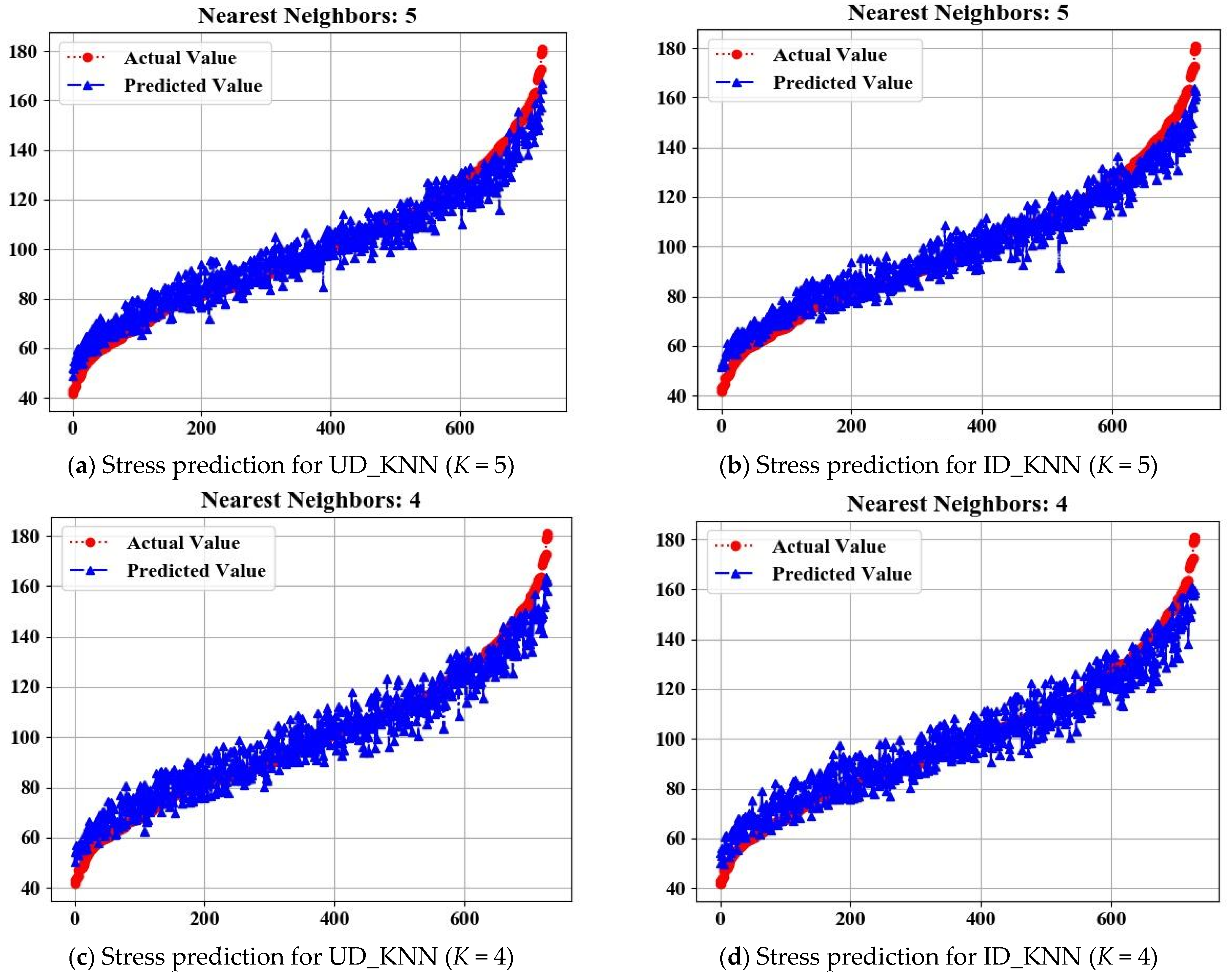
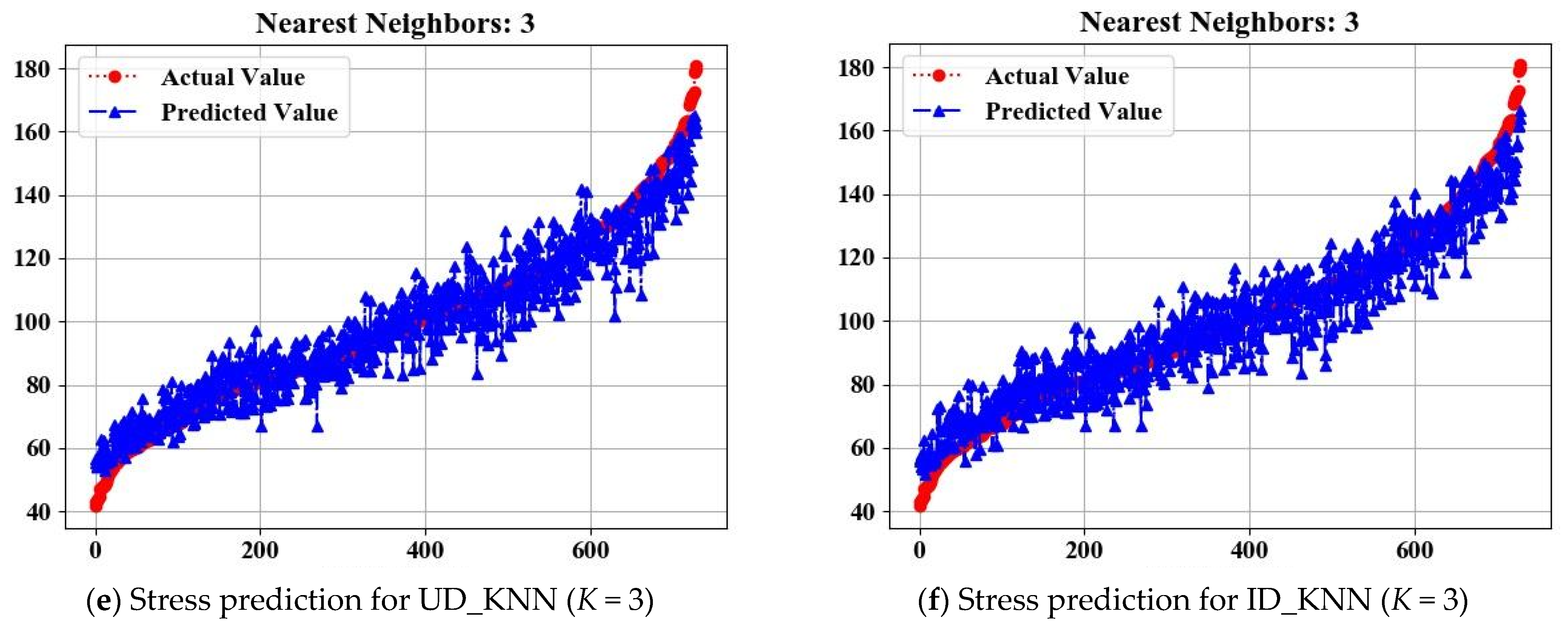
Table 3 compares the performance evaluations using two KNNR methods: UD and ID.
The dataset consists of stress and strain measurements obtained from FEM modeling and the ML model runs on the dataset provided by the FEM, along with corresponding input features. KNN regression models were trained using two weighting schemes: UD- and ID-based. The number of neighbors, K, was varied (3, 4, and 5) to examine its impact on model performance (see
Figure 10a–f for strain predictions, and
Figure 11a–f for stress predictions). Performance metrics including R
2, MAE, MAE/Ave (%), RMSE, and RMSE/Ave (%) were calculated to evaluate the accuracy and generalization capabilities of the models. The results in
Table 3 indicate that both UD- and ID-based KNN regression models perform well in predicting stress and strain values, with R
2 values ranging from 0.91 to 0.956 across different configurations. Generally, the models exhibit low mean absolute error (MAE) and root mean squared error (RMSE) values, indicating good accuracy in predicting stress and strain. The performance metrics also show slight variations based on the number of neighbors (K) and the weighting scheme employed.
5.4. XML Results
The SHAP summary plot in
Figure 12 highlights the contribution of each feature to the prediction of maximum stress, as measured by the mean absolute SHAP values. The mean absolute SHAP values measure the contribution of each feature to the prediction of the target variable (equivalent maximum stress in
Figure 11).
The Pressure Magnitude (P4) is the most influential feature, with a mean SHAP value of +17.42, indicating it has the largest impact on the target variable. The feature P3-d follows with a significant contribution of +11.45, showing its strong influence as well. In contrast, Young’s Moduli in the X direction (P12), Z direction (P14), and Y direction (P13) have moderate effects, with SHAP values of +8.22, +5.76, and +4.22, respectively. Interestingly, Poisson’s Ratio XY (P15) has a minimal impact, contributing only +0.38, suggesting it plays a negligible role in determining the maximum stress. This analysis shows that the pressure magnitude dominates as the key predictor, while the elastic properties of the material have a secondary but notable influence.
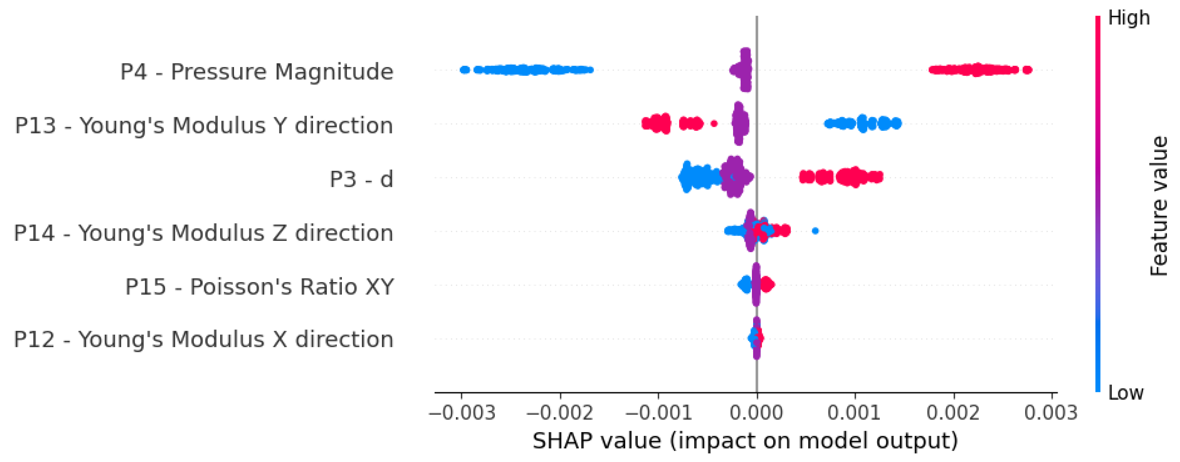
Figure 13 presents a SHAP value analysis of various mechanical properties and their impact on equivalent maximum stress, particularly revealing the directionality (positive and negative) and granularity (the effect of each data point) for each feature. The visualization reveals that P4 (Pressure Magnitude) and P3 (d) exhibit the strongest influence on the model’s predictions, with SHAP values ranging from approximately −30 to +20. Interestingly, high values of the pressure magnitude (shown in red) contribute positively to the model output, while lower values (in blue) have a negative impact. The Young’s Modulus values in three orthogonal directions (X, Y, and Z) demonstrate a moderate influence, with their impact being relatively symmetric around zero but showing distinct directional effects—higher values tend to increase the predicted stress (positive SHAP values), while lower values decrease it (negative SHAP values). The visualization also reveals that P15 (Poisson’s Ratio XY) has the lowest impact on the model output, with SHAP values concentrated near zero, suggesting minimal directional influence on the stress predictions. This bidirectional relationship between feature values and their impact provides insights into how each parameter either amplifies or reduces the predicted equivalent maximum stress, with the magnitude and direction of influence varying significantly across different mechanical properties.
Figure 14 presents the average absolute SHAP values for different mechanical properties and their influence on equivalent maximum strain predictions. The Pressure Magnitude (P4) demonstrates the most substantial impact on strain predictions, with a mean absolute SHAP value of approximately 0.0016, indicating its dominant role in determining strain outcomes. Young’s Modulus in the
Y direction (P13) shows the second-highest influence, followed closely by the dimensional parameter d (P3), with mean absolute SHAP values of about 0.0007 and 0.0006, respectively. Young’s Modulus in the
Z direction (P14), Poisson’s Ratio XY (P15), and Young’s Modulus in the
X direction (P12) exhibit relatively minor influences on strain predictions, with mean absolute SHAP values far below 0.0002.
Figure 15 presents a SHAP value plot explaining the influence of various mechanical properties on equivalent maximum strain predictions. The Pressure Magnitude (P4) exhibits the most pronounced impact, with SHAP values ranging from approximately −0.003 to +0.002, showing a clear bidirectional effect, where lower pressures (blue) contribute to strain reduction and higher pressures (red) to strain increase. Young’s Modulus in the Y direction (P13) and the dimensional parameter d (P3) demonstrate moderate influences, with their distributions suggesting complex interactions. Higher values of Young’s Modulus Y (red) appear near zero and negative SHAP values, while lower values (blue) contribute to positive strain predictions. Young’s Modulus in the Z direction (P14), Poisson’s Ratio XY (P15), and Young’s Modulus in the X direction (P12) show relatively concentrated distributions around zero, indicating minimal impact on strain predictions. The visualization effectively captures both the magnitude and directionality of each parameter’s influence, with feature values color-coded from low (blue) to high (red), providing insights into how these mechanical properties collectively influence the model’s strain predictions.
6. Conclusions
This research presented the design of carbon-carbon (C-C) composites under uncertainty, particularly focusing on their application in ultra-high temperature environments such as concentrating solar power (CSP) collectors. The integration of finite element modeling (FEM), classic machine learning (ML), and explainable ML (XML) has paved the way for the development of reliable and explainable models, essential for optimizing the design of C-C composite components.
Uncertainty-based analysis of the mechanical characterization of C-C composites underscored the multifaceted challenges inherent in their design for every component intended for ultra-high temperature applications.
This study focuses on using synthetic data generated by FEM to train ML and XML algorithms for analyzing and explaining C-C composite behavior at ultra-high temperatures. Particular emphasis is placed on the novel carbonized microvascular C-C composite, designed for use as a microvascular receiver in advanced CSP collectors. Leveraging microVasc technology, a solar receiver is engineered as a lightweight, high-absorptivity material featuring an embedded microvascular network. This solar receiver possesses the capability of being optimized for heat transfer to a supercritical carbon dioxide (sCO2) heat transfer fluid. The utilization of ANSYS 3-D FEM facilitated a comprehensive investigation into the stress and strain analysis within C-C composite CSP collectors. Recognizing the variability in the mechanical and thermal properties inherent in C-C composites, over 730 ANSYS simulations were conducted to generate a synthetic dataset for ML algorithms and XML analysis, enabling uncertainty analysis and prediction.
The accurate determination of the Poisson’s ratio magnitude for C-C composites presents a challenge due to its potential influence on stress and strain. Yet, the sensitivity analysis based on data correlation unveils that the precise quantification of this parameter is not pivotal in the stress/strain analysis of C-C composite CSP collectors, offering a degree of respite in the composite design endeavor. Nevertheless, it is paramount to recognize the limitations of the current analysis, as its applicability may not universally extend to all components featuring C-C composites across diverse boundary conditions. Particularly within the realm of dynamic and highly nonlinear loading scenarios, the complexities of Poisson’s ratio may unfold in multifaceted manners.
K-Nearest neighbors (KNN) regressions were employed based on two voting systems of uniform direct distance (UD) and inverse distance (ID). Both the UD and ID-based KNN regression models displayed an acceptable performance in predicting the stress and strain values where the R2 values ranged from 0.91 to 0.956. The mean absolute error (MAE) and root mean squared error (RMSE) were lower than 10% for all calculations. Additionally, the performance metrics indicated slight variations based on the number of neighbors (K) and the weighting scheme used in this study. Furthermore, SHAP (SHapley Additive exPlanations) was employed to improve the predictive model’s explainability. The XML model helped to quantitatively measure each feature’s contribution to individual predictions of strain and stress. This research both contributes to the advancement of C-C composite technology and highlights the potential of interdisciplinary approaches combining FEM, ML, XML, and uncertainty analysis to address complex engineering challenges, particularly where ultra-high temperature is critical. The results of this research can be used as a benchmark to advance the practical application of C-C composites in high-temperature environments.
Author Contributions
Conceptualization, V.D., H.D. and M.W.K.; Methodology, H.D.; Software, H.D.; Validation, V.D. and H.D.; Formal analysis, V.D.; Investigation, V.D. and M.W.K.; Resources, M.W.K.; Writing—original draft, V.D.; Writing—review & editing, V.D., H.D. and M.W.K.; Supervision, V.D. and M.W.K. All authors have read and agreed to the published version of the manuscript.
Funding
This work was supported in part by the US Department of Energy Solar Energy Technologies Office under award number DE-EE0008736.
Data Availability Statement
The data presented in this study are being utilized in an ongoing research project. Upon completion of the study, the data may be available upon request from the corresponding author.
Conflicts of Interest
The authors declare no conflict of interest.
References
- Zuzelski, M.; Laporte-Azcué, M.; Cordeiro, J.; Dhakal, S.; Daghigh, V.; Keller, M.; Ramsurn, H.; Otanicar, T. Design of a novel carbon/carbon composite microvascular solar receiver. Sol. Energy 2023, 262, 111794. [Google Scholar] [CrossRef]
- Kiss, G. Solar energy in the built environment: Powering the sustainable city. In Metropolitan Sustainability; Elsevier: Amsterdam, The Netherlands, 2012; pp. 431–456. [Google Scholar] [CrossRef]
- Sarbu, I.; Sebarchievici, C. Solar Collectors. In Solar Heating and Cooling Systems; Elsevier: Amsterdam, The Netherlands, 2017; pp. 29–97. [Google Scholar] [CrossRef]
- Brown, T. Heat Transfer Modeling and Optimization of a Carbonized Microvascular Solar Receiver. Master’s Thesis, Boise State University, Boise, ID, USA, 2020. [Google Scholar] [CrossRef]
- Solar|OSU Energy Efficiency Center|Oregon State University. Available online: https://eec.oregonstate.edu/solar (accessed on 1 February 2025).
- Du, S.; Wang, Z.; Shen, S. Thermal and structural evaluation of composite solar receiver tubes for Gen3 concentrated solar power systems. Renew Energy 2022, 189, 117–128. [Google Scholar] [CrossRef]
- Mehos, M.; Turchi, C.; Vidal, J.; Wagner, M.; Ma, Z.; Ho, C.; Kolb, W.; Andraka, C.; Kruizenga, A. Concentrating Solar Power Gen3 Demonstration Roadmap; National Renewable Energy Laboratory (NREL): Golden, CO, USA, 2017. [CrossRef]
- Soffel, F.; Eisenbarth, D.; Hosseini, E.; Wegener, K. Interface strength and mechanical properties of Inconel 718 processed sequentially by casting, milling, and direct metal deposition. J. Mater. Process Technol. 2021, 291, 117021. [Google Scholar] [CrossRef]
- Alojaly, H.M.; Hammouda, A.; Benyounis, K.Y. Review of Recent Developments on Metal Matrix Composites with Particulate Reinforcement. In Comprehensive Materials Processing, 2nd ed.; Elsevier: Amsterdam, The Netherlands, 2024; pp. 350–373. [Google Scholar] [CrossRef]
- Djugum, R.; Sharp, K. The fabrication and performance of C/C composites impregnated with TaC filler. Carbon 2017, 115, 105–115. [Google Scholar] [CrossRef]
- Zweben, C. Materials: Composites. In Encyclopedia of Condensed Matter Physics, 2nd ed.; Elsevier: Amsterdam, The Netherlands, 2024; pp. 333–349. [Google Scholar] [CrossRef]
- Daghigh, V.; Belk, D.M.; Nikbin, K. Development and validation of finite element models for buckling of open-hole fiber-reinforced composites at ambient and cryogenic temperatures. Phys. Scr. 2023, 98, 025702. [Google Scholar] [CrossRef]
- Windhorst, T.; Blount, G. Carbon-carbon composites: A summary of recent developments and applications. Mater. Des. 1997, 18, 11–15. [Google Scholar] [CrossRef]
- Oku, T. Carbon/Carbon Composites and Their Properties. In Carbon Alloys; Elsevier: Amsterdam, The Netherlands, 2003; pp. 523–544. [Google Scholar] [CrossRef]
- Karadimas, G.; Salonitis, K. Ceramic Matrix Composites for Aero Engine Applications—A Review. Appl. Sci. 2023, 13, 3017. [Google Scholar] [CrossRef]
- Shan, Y.; Liao, K. Environmental fatigue of unidirectional glass–carbon fiber reinforced hybrid composite. Compos. Part B Eng. 2001, 32, 355–363. [Google Scholar] [CrossRef]
- Daghigh, V.; Khalili, S.M.R.; Eslami Farsani, R. Creep behavior of basalt fiber-metal laminate composites. Compos. Part B Eng. 2016, 91, 275–382. [Google Scholar] [CrossRef]
- Ghorbani, J.; Daghigh, V.; Rahmati, S.; Mahdian, M.; Daghigh, H. Creep behavior of latania natural fiber-reinforced epoxy composites at elevated temperatures. Polym. Compos. 2021, 42, 3089–3097. [Google Scholar] [CrossRef]
- Craig, W.O.; Wallace, L.V.; Philip, O.R.; Hwa-Tsu, T. Thermal Conductivity Database of Various Structural Carbon-Carbon; NASA Langley: Hampton, VA, USA, 1997.
- Rymal, C. Numerical Design of a High-Flux Microchannel Solar Receiver. Master’s Thesis, Oregan State University, Corvallis, OR, USA, 2014. [Google Scholar]
- Rymal, C.J.; Apte, S.V.; Narayanan, V.; Drost, K. Numerical Design of a Planar High-Flux Microchannel Solar Receiver. In Proceedings of the ASME 2014 8th International Conference on Energy Sustainability, Boston, MA, USA, 30 June–2 July 2014; p. V001T02A050. [Google Scholar] [CrossRef]
- Keller, M.; Ramsurn, H.; Crunkleton, D.; Daghigh, V.; Cordeiro, C.; Argot, J. Carbon-Based Receiver Systems are a Potential Alternative to Metal-Based Receiver Systems; Office of Energy Efficient & Renewable Energy, US Department of Energy: Washington, DC, USA, 2021.
- Daghigh, V.; Daghigh, H.; Lacy, T.E.; Naraghi, M. Review of machine learning applications for defect detection in composite materials. Mach. Learn Appl. 2024, 18, 100600. [Google Scholar] [CrossRef]
- Daghigh, V.; Lacy, T.E., Jr.; Daghigh, H.; Gu, G.; Baghaei, K.T.; Horstemeyer, M.F.; Pittman, C.U., Jr. Heat deflection temperatures of bio-nano-composites using experiments and machine learning predictions. Mater. Today Commun. 2020, 22, 100789. [Google Scholar] [CrossRef]
- Fletcher, R.G. Geographic Information Systems in Real Estate. In Encyclopedia of Information Systems; Elsevier: Amsterdam, The Netherlands, 2003; pp. 433–441. [Google Scholar] [CrossRef]
- Daghigh, V.; Naraghi, M. Machine learning-based defect characterization in anisotropic materials with IR-thermography synthetic data. Compos. Sci. Technol. 2023, 233, 109882. [Google Scholar] [CrossRef]
- Oviedo, F.; Ferres, J.L.; Buonassisi, T.; Butler, K.T. Interpretable and Explainable Machine Learning for Materials Science and Chemistry. Acc. Mater. Res. 2022, 3, 597–607. [Google Scholar] [CrossRef]
- Zhong, X.; Gallagher, B.; Liu, S.; Kailkhura, B.; Hiszpanski, A.; Han, T.Y.-J. Explainable machine learning in materials science. NPJ Comput. Mater. 2022, 8, 204. [Google Scholar] [CrossRef]
- Roscher, R.; Bohn, B.; Duarte, M.F.; Garcke, J. Explainable Machine Learning for Scientific Insights and Discoveries. IEEE Access 2020, 8, 42200–42216. [Google Scholar] [CrossRef]
- Belle, V.; Papantonis, I. Principles and Practice of Explainable Machine Learning. Front. Big Data 2021, 4, 688969. [Google Scholar] [CrossRef] [PubMed]
- Daghigh, V.; Bakhtiari Ramezani, S.; Daghigh, H.; Lacy Jr, T.E. Explainable artificial intelligence prediction of defect characterization in composite materials. Compos. Sci. Technol. 2024, 256, 110759. [Google Scholar] [CrossRef]
- Rokach, L.; Maimon, O. Decision Trees. In Data Mining and Knowledge Discovery Handbook; Maimon, O., Rokach, L., Eds.; Springer: New York, NY, USA, 2005; pp. 165–192. [Google Scholar] [CrossRef]
- Daghigh, V. Mechanical and Thermal Behavior of Multiscale Bi-Nano-Composites Using Experiments and Machine Learning Predictions. Ph.D. Thesis, Mississippi State University, Mississippi State, MS, USA, 2020. [Google Scholar]
- Daghigh, V.; Lacy, T.E., Jr.; Daghigh, H.; Gu, G.; Baghaei, K.T.; Horstemeyer, M.F.; Pittman, C.U., Jr. Machine learning predictions on fracture toughness of multiscale bio-nano-composites. J. Reinf. Plast. Compos. 2020, 39, 587–598. [Google Scholar] [CrossRef]
- Zuzelski, M. Carbon/Carbon Composites for Next Generation Microvascular Solar Thermal Receivers. Master of Science in Mechanical Engineering. Master’s Thesis, Boise State University, Boise, ID, USA, 2023. [Google Scholar] [CrossRef]
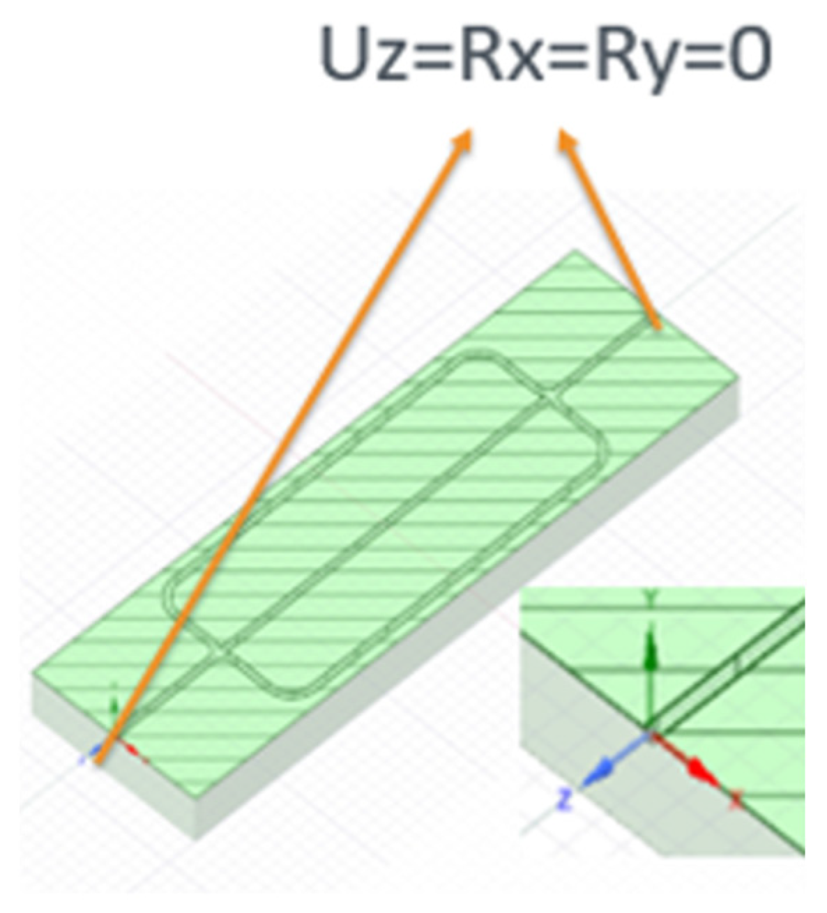
Figure 1.
Schematic view of the C-C composite concentrating solar power collector and mechanical boundary conditions (the microchannel format was inspired by [
4,
20,
21,
22]). (Note: U represents displacement, and R represents rotation).
Figure 1.
Schematic view of the C-C composite concentrating solar power collector and mechanical boundary conditions (the microchannel format was inspired by [
4,
20,
21,
22]). (Note: U represents displacement, and R represents rotation).
Figure 2.
KNN regression analysis. The red circle represents the neighborhood area of interest.
Figure 2.
KNN regression analysis. The red circle represents the neighborhood area of interest.
Figure 3.
Overview of training and testing set divisions using k-fold cross-validation, depicting data division into k segments (k = 5).
Figure 3.
Overview of training and testing set divisions using k-fold cross-validation, depicting data division into k segments (k = 5).
Figure 4.
Temperature distribution over the C-C composite; a quartered model where the top and bottom surfaces are set to be 851 °C and 586 °C, respectively.
Figure 4.
Temperature distribution over the C-C composite; a quartered model where the top and bottom surfaces are set to be 851 °C and 586 °C, respectively.
Figure 5.
Equivalent stress distribution over the C-C composite; (a) half of the quarter model, (b) magnified image of the area with the maximum stress.
Figure 5.
Equivalent stress distribution over the C-C composite; (a) half of the quarter model, (b) magnified image of the area with the maximum stress.
Figure 6.
Equivalent alternating stress distribution over the C-C composite; (a,b) the quarter model, and half of the quarter model with the magnified area containing maximum stress.
Figure 6.
Equivalent alternating stress distribution over the C-C composite; (a,b) the quarter model, and half of the quarter model with the magnified area containing maximum stress.
Figure 7.
Equivalent elastic strain over the C-C composite; (a) the quarter model, (b) half of the quarter model with the magnified area containing maximum stress.
Figure 7.
Equivalent elastic strain over the C-C composite; (a) the quarter model, (b) half of the quarter model with the magnified area containing maximum stress.
Figure 8.
Biaxiality indication for stress distribution over the C-C composite; (a) the quarter model, and (b) half of the quarter model.
Figure 8.
Biaxiality indication for stress distribution over the C-C composite; (a) the quarter model, and (b) half of the quarter model.
Figure 9.
Correlation coefficients considering six inputs and two outputs.
Figure 9.
Correlation coefficients considering six inputs and two outputs.
Figure 10.
Actual equivalent strain data generated by finite element versus predicted data by machine learning; the left column contains the UD_KNN, and the right column contains the ID_KNN (strain is represented in mm/mm, indicating its dimensionless nature).
Figure 10.
Actual equivalent strain data generated by finite element versus predicted data by machine learning; the left column contains the UD_KNN, and the right column contains the ID_KNN (strain is represented in mm/mm, indicating its dimensionless nature).
Figure 11.
Actual equivalent stress data generated by finite element versus predicted data by machine learning; the left column contains the UD_KNN, and the right column contains the ID_KNN (the stress unit is MPa).
Figure 11.
Actual equivalent stress data generated by finite element versus predicted data by machine learning; the left column contains the UD_KNN, and the right column contains the ID_KNN (the stress unit is MPa).
Figure 12.
SHAP summary plot, showing the feature importance for predicting maximum stress. The mean absolute SHAP values quantify the impact of each feature on the model’s output (equivalent maximum stress).
Figure 12.
SHAP summary plot, showing the feature importance for predicting maximum stress. The mean absolute SHAP values quantify the impact of each feature on the model’s output (equivalent maximum stress).
Figure 13.
Distribution of SHAP values showing the magnitude and directional influence of mechanical properties on equivalent maximum stress predictions, with feature values indicated by color gradient (blue: negative to red: positive).
Figure 13.
Distribution of SHAP values showing the magnitude and directional influence of mechanical properties on equivalent maximum stress predictions, with feature values indicated by color gradient (blue: negative to red: positive).
Figure 14.
Mean absolute SHAP values illustrate the relative importance of mechanical properties in predicting equivalent maximum strain. The bar lengths represent the average magnitude of influence for each parameter, with all properties showing absolute contributions to the model’s equivalent maximum strain predictions.
Figure 15.
SHAP value distributions show the magnitude, direction, and feature–value relationships of mechanical properties’ effects on equivalent maximum strain predictions.
Figure 15.
SHAP value distributions show the magnitude, direction, and feature–value relationships of mechanical properties’ effects on equivalent maximum strain predictions.
Table 1.
Comparison of C-C composites, C-SiC composites, and CFRP.
Table 1.
Comparison of C-C composites, C-SiC composites, and CFRP.
| Property | C-C Composites | C-SiC Composites | CFRP |
|---|
| Thermal Stability | Excellent (up to 3000 °C in inert environments) | Good (~1600 °C) | Poor (~150–300 °C) |
| Oxidation Resistance | Poor (requires protective coatings) | Excellent (due to SiC matrix) | Not a major concern |
| Strength-to-Weight Ratio | High | Moderate | Very High |
| Temperature Limit | 3000 °C | 1600 °C | 300 °C |
| Cost | High | Very High | Low |
| Applications | Rocket nozzles, thermal shields, and extreme high-temperature applications | Aerospace, automotive braking systems, turbine engines | Automotive, sports equipment, structural aerospace components |
Table 2.
Mechanical and thermal properties of carbon-carbon composites used in the ANSYS FEA [
1,
19].
Table 2.
Mechanical and thermal properties of carbon-carbon composites used in the ANSYS FEA [
1,
19].
| Density (kg/m3) | 2260 | | |
| Young’s Modulus X direction (Pa) | 4.0 × 10¹¹ | | |
| Young’s Modulus Y direction (Pa) | 2.0 × 10¹¹ | | |
| Young’s Modulus Z direction (Pa) | 2.0 × 10¹¹ | | |
| Poisson’s Ratio XY | 3.0 × 10⁻¹ | | |
| Poisson’s Ratio YZ | 3.0 × 10⁻¹ | | |
| Poisson’s Ratio XZ | 3.0 × 10⁻¹ | | |
| Shear Modulus XY (Pa) | 7.5 × 10⁹ | | |
| Shear Modulus YZ (Pa) | 5.5 × 10⁹ | | |
| Shear Modulus XZ (Pa) | 7.5 × 10⁹ | | |
| Tensile Yield Strength (Pa) | 2.5 × 10⁸ | | |
| Compressive Yield Strength (Pa) | 2.5 × 10⁸ | | |
| | at T = 800 K | at T = 900 K | at T = 1300 K |
| Thermal Conductivity X direction (W/mK) | 21.0 | 19.5 | 19.5 |
| Thermal Conductivity Y direction (W/mK) | 8.0 | 7.5 | 9 |
| Thermal Conductivity Z direction (W/mK) | 21.0 | 19.5 | 19.5 |
Table 3.
Comparison of performance evaluations using two KNNR methods: uniform distance (UD) and inverse distance (ID).
Table 3.
Comparison of performance evaluations using two KNNR methods: uniform distance (UD) and inverse distance (ID).
| KNN | Weight | Output | R2 | MAE | MAE/Ave (%) | RMSE | RMSE/Ave (%) |
|---|
| 3 | uniform | Stress | 0.918 | 6.3798753 | 6.403 | 8.053662 | 8.084 |
| 3 | uniform | Strain | 0.951 | 0.000356 | 5.301 | 0.000486 | 7.251 |
| 4 | uniform | Stress | 0.934 | 5.722474 | 5.744 | 7.169652 | 7.197 |
| 4 | uniform | Strain | 0.947 | 0.000403 | 6.013 | 0.000512 | 7.626 |
| 5 | uniform | Stress | 0.942 | 5.424475 | 5.445 | 6.760849 | 6.787 |
| 5 | uniform | Strain | 0.95 | 0.000394 | 5.871 | 0.000491 | 7.314 |
| 3 | inverse | Stress | 0.91 | 6.804146 | 6.830 | 8.415996 | 8.448 |
| 3 | inverse | Strain | 0.956 | 0.000338 | 5.044 | 0.000459 | 6.844 |
| 4 | inverse | Stress | 0.932 | 5.855529 | 5.878 | 7.326903 | 7.355 |
| 4 | inverse | Strain | 0.948 | 0.000393 | 5.856 | 0.0005 | 7.452 |
| 5 | inverse | Stress | 0.945 | 5.253027 | 5.273 | 6.603391 | 6.629 |
| 5 | inverse | Strain | 0.953 | 0.000377 | 5.620 | 0.000479 | 7.134 |
| Disclaimer/Publisher’s Note: The statements, opinions and data contained in all publications are solely those of the individual author(s) and contributor(s) and not of MDPI and/or the editor(s). MDPI and/or the editor(s) disclaim responsibility for any injury to people or property resulting from any ideas, methods, instructions or products referred to in the content. |
© 2025 by the authors. Licensee MDPI, Basel, Switzerland. This article is an open access article distributed under the terms and conditions of the Creative Commons Attribution (CC BY) license (https://creativecommons.org/licenses/by/4.0/).


