Abstract
Due to the versatility of its implementation, additive manufacturing has become the enabling technology in the research and development of innovative engineering components. However, many experimental studies have shown inconsistent results and have highlighted multiple defects in the materials’ structure thus bringing the adoption of the additive manufacturing method in practical engineering applications into question, yet limited work has been carried out in the material modelling of such cases. In order to account for the effects of the accumulated defects, a micromechanical analysis based on the representative volume element has been considered, and phase-field modelling has been adopted to model the effects of inter-fiber cracking. The 3D models of representative volume elements were developed in the Abaqus environment based on the fiber dimensions and content acquired using machine learning algorithms, while fulfilling both geometric and material periodicity. Furthermore, the periodic boundary conditions were assumed for each of the representative volume elements in transversal and in-plane shear test cases,. The analysis was conducted by adopting an open-source UMAT subroutine, where the phase-field balance equation was related to the readily available heat transfer equation from Abaqus, avoiding the necessity for a dedicated user-defined element thus enabling the adoption of the standard elements and features available in the Abaqus CAE environment. The model was tested on three representative volume element sizes and the interface properties were calibrated according to the experimentally acquired results for continuous carbon-fiber-reinforced composites subjected to transverse tensile and shear loads. This investigation confirmed the consistency between the experimental results and the numerical solutions acquired using a phase-field fracture approach for the transverse tensile and shear behavior of additively manufactured continuous-fiber-reinforced composites, while showing dependence on the representative volume element type for distinctive load cases.
1. Introduction
Additive manufacturing (AM) technology of polymeric materials has more frequently been adopted in engineering applications [1,2], especially for prototyping in research and development [2,3], with prospects in mold tooling and tool jigs, limited-run production parts, service parts, maintenance and repair, and lightweight solutions in automotive industries [4,5,6], as well as in medical applications [7,8,9]. A comprehensive review aiming to synthesize the most relevant studies on carbon-based nano-composites was conducted in [10]. The authors discuss the mechanical and electrical properties of materials reinforced with carbonaceous nanofillers, such as graphene nanoplatelets and carbon nanotubes, and their compatibility with the requirements for biomedical applications, emphasizing the potential of the specific electrical, thermal, and mechanical properties of CNTs fillers in multifunctional, hight-strength, lightweight, and self-lubricating wear resistant composites. In addition, a comprehensive review on graphene nanofillers in metal matrix composites for biomedical applications was conducted in [11], highlighting the influences of nano-additive phases on cytotoxicity and the tailored mechanical properties achieved in implants by adopting scaffold structures. All thing considered, the application of AM technology was also further extended by the introduction of particle or fiber fillers to achieve the beneficial properties of these reinforcing materials. The prospects of embedding nanofillers in additively manufactured composite materials were investigated in [12], highlighting the increased strength and stiffness achieved when the components are reinforced with fibers and fillers, which led to a significant amount of research being concentrated on material selection and enhancing the characteristics of cost-effective printed components [12]. However, the experimental observations on the behavior of these enhanced materials show inconsistency with the performance of their conventionally manufactured counterparts [13,14,15], which has also been found as one of the major obstacles to the adoption of AM in the current industries [16]. A comprehensive review of the application of AM composites has been revied in [17], highlighting its potential in medical applications. A comprehensive review of the application of AM composites has been revied in [17], while the enhancement of the dielectric and thermal properties of polymeric composites by the addition of fillers was investigated in [18,19] respectively. The mechanical properties of carbon-fiber-reinforced specimens containing various LSSs were studied in [20]. While these reinforced materials exhibit heterogeneity, the AM components manifest in manufacturing inherent deposition deficiencies which are often attributed to the microscopic voids and inclusion [15,21,22]. Among these defects, the AM parts also depend on various controllable manufacturing parameters as well as the mechanical properties of the constituents, which often results in data inconsistencies and issues uncertainty in the prediction of the material behavior. These FDM-induced flaws were further studied in [21,22,23], indicating the necessity for microscopic analysis and NDT component examinations, as well as quantification of the deficiencies which affect the mechanical behavior of AM CFRP composites; however, the modelling approaches which account for the effects of the AM process are limited.
In order to calculate the resulting material properties in novel composite AM extrusion mixtures, microstructural analysis of these heterogenic materials is essential. This can be achieved by analyzing a representative volume element (RVE) designed according to the available microstructural information on the constituents’ geometries and behaviors, as shown in [24,25,26,27], as well as being proven valid in multiple studies [28,29,30,31,32,33]. The constituents’ geometry can be acquired from 2D microscopy [13,34] and then prepared using AI-thresholding [35] for statistical evaluations, based on which, and some assumptions, the RVE is built or it can be analyzed from the 3D µCT scans [36,37] using the voxel approach [38]. Such models are prepared in a CAE environment where each of the constituents adopts its constitutive behavior. Since these material models are usually acquired from macroscale analyses, additional assumptions on the inter-material contact behavior [13,28,39,40] have to be adopted. In commercial FEA software, these interactions are implemented using cohesive elements [28] or alternatively using phase-field modelling [39,40,41].
The phase field approach was initially developed to overcome the problems of moving interface boundaries and topology adjustments when simulating the morphologies of evolving interfaces in cases of merging or division [42,43]. Based on the initial formulations presented in [44,45], the model uses a set of field variables Φ which are described using partial differential equations (PDEs) and they distinguish the two phases (0 and 1), between which a smooth transition is assumed when calculated in the proximity of the interface [46]. These sets of variables are continuous functions of time and spatial coordinates and can be integrated without explicit treatment of interface conditions [42,43]. By adopting the thermodynamic free energy approach, the phase field evolution can be defined in terms of temperature, strain, or concentration to predict various changes in microstructural features, leading to frequent application in simulations of microstructural evolutions [47] and the modelling of fracture mechanics [48].
Since complex crack trajectories and crack branching [49] can be achieved with arbitrary geometries and dimensions without tempering with the FE mesh, the application of this approach has been adopted for modelling various complex phenomena [49] including stress and temperature-induced transformations in shape memory alloys [50], functionally graded materials [51,52], hyper-elastic materials [53,54], compressive shear fracture in basalt, cement mortar and sandstone [55], chemo-mechanically assisted fractures [56], hydrogen embrittled alloys [57], piezoelectric [58], and fiber-reinforced composites [59,60]. However, despite still being limited in engineering applications, there are several reported applications in commercial FEA software including MATLAB [61,62,63], Python [64,65], Abaqus [46,50,57,66,67,68,69,70,71], and COMSOL [55,72], many of which are published in open-source archives. The constitutive relations used in these phase-field implementations are based on [45,73] as the AT2 and the AT1 model, respectively, and some of the presented implementations include the regularized cohesive zone model PF-CZM based on [74,75,76,77] while adopting newton monolithic [57], one-pass AM/staggered [57], or iterative AM/staggered solver algorithms [71] for acquiring solutions [49].
Furthermore, the development of solution algorithms for the coupled deformation-fracture problem was presented in [49,57,78,79]. The total potential energy is minimized according to the displacement field u and phase field Φ, while Φ is solved as a damage variable [80] at the finite element node instead of at the integration point as in cases of local damage models [46]. This is achieved using a user-defined element (UEL) prior to the implementation of the user defined material model (UMAT), which limits the modelling and visualization capabilities of commercial software [46]. This has been accounted for in [46,80] by adopting the similarity between the phase field balance and heat transfer equations which enables the calculation of phase-field damage Φ variable as an additional degree of freedom without the necessity for the UEL mesh definition. To retain all of the the Abaqus built-in modelling and meshing features, this approach has been implemented for the micromechanical damage modelling of AM carbon fiber-reinforced thermoplastic polymer (CFRP) composite RVE and validated on experimentally acquired data. All things considered, this work is focused on the application of the phase field approach in modelling the microstructural failure of AM CFRP composite RVE subjected to tensile and shear loads. Therefore, as an extension to the previously published work where the RVEs were modelled based on continuum mechanics and cohesive finer/matrix interfaces [13,81], the behavior of the AM CFRP composite was modelled in this work using a phase field modelling approach, introducing microscopic damage and showing better scalability of the RVE based on microscopic imaging in contrast to the previously acquired results in [13,81].
2. Materials and Methods
The consistency of an AM material may vary due to the ratios and microscopic properties of the constituents, the chemical properties of the sizing agents, layer thickness, nozzle diameter, humidity, filling type, and density, as well as the extrusion speed and temperature [82]. Since many of these parameters could be controlled, an iterative design process in novel material development is essential. Therefore, a micromechanical modelling approach based on the representative volume element has been proposed in this work.
The CFRP composite specimens for microscopic analysis were designed as 12 layered 25 × 25 mm laminated plates with a cross-ply stacking sequence equal to [0/902/0/902]s, as shown in Figure 1, and additively manufactured using a Markforged X7 3D printer. This LSS was adopted after a preliminary microstructural examination of similar AM composites. A similar LSS is used in acquiring the multiaxial response through uniaxial tensile tests on rectangular specimens [83], which was also studied in [14]. This sequence also enables the measurements of unidirectionally reinforced layer composition and gives a better insight into laminar dimensions, layer-wise defect accumulation, and repeatability issues between single, double, and multiple adjacent layers. However, these specimens did not account for the lengthwise defect accumulation due to uneven material solidification.
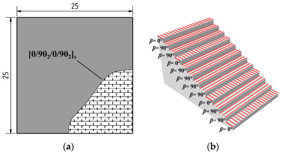
Figure 1.
CFRP laminate sample [81]: (a) sketch in the x-y plane, and (b) LSS details.
The specimens were then cut along and perpendicular to the dominant fiber direction in order to acquire x-z and y-z cross-sections, while the x-y cross-section is acquired by grinding the polymeric top layer of the specimens. The cross-sections were polished and prepared for observation using the FEI-QUANTA-250-FEG scanning electron microscope. The acquired images were inspected and, due to the ununiform matrix background, the images were segmented based on pixel classification using Trainable WEKA segmentation machine learning algorithms which are readily available in FIJI [35] open-source software. The acquired results were statistically evaluated and compared with the data available in the relevant literature. Following the comparison, the RVEs were designed according to [13,31,84], while adopting the microscopic properties acquired from the four middle layers. The first case (RVE-1) was designed as a single fiber unit cell; the rectangular and hexagonal fiber arrangements have been adopted for the second (RVE-2) and the third (RVE-3), respectively, while keeping the smallest possible RVE size for the measured fiber volume ratio to increase the computational efficiency. However, to acquire more accurate results from the analysis of small-size RVEs, the fibers were placed at the RVE boundary edges [84], while ensuring geometrical, material, and mesh periodicity [13,31]. This was adopted for the cases of rectangular and hexagonal fiber arrays, while for the unit-cell case, both conditions could not be fulfilled.
In order to distinguish between the fiber, the matrix, and the fiber/matrix interface behaviors, each RVE domain was divided into three subdomains. The model was discretized using coupled temperature-displacement hexahedral elements (C3D8T), with the predefined temperature field indicating the initial state of damage within the material. Furthermore, the linear elastic behavior was assumed for the phase field damage framework [33], while the fiber and matrix’s mechanical properties were adopted from [85] and [86], respectively; as shown in Table 1. The constituents’ properties were adopted from the literature since the commercially available data are available only for the UD composite reinforced in the direction of the layers with the elastic modulus of 60 GPa and tensile strength of 800 MPa [87], while the matrix data are available for the AM polymer used in the secondary nozzle, and not in the analyzed CFRP material. The toughness K1C was adopted for polyamide according to [88] and recalculated to acquire the GC values. In contrast to the fiber and the matrix, the values for the interface properties were assumed and calibrated according to the experimentally observed material behavior.

Table 1.
Constituents’ mechanical properties.
In order to appropriately simulate the behavior of the surrounding material, periodic boundary conditions (PBC) have been enforced on the RVEs boundary corners, edges, and surfaces [28,30,31,32,33], where the PBCs and the node constrain equations were defined using the automated procedure presented in [31,32]. However, instead of focusing on extracting the elastic properties, the procedure was modified to calculate the material degradation and damage using user-defined subroutines and simulate the complete material response until failure.
The mesh sensitivity was studied on three distinctive cases of RVEs with assumed hexahedral fiber placement. The curvature maximal deviation factor h/L was assumed as 0.01 for each of the tested cases, while the approximate element sizes were adopted as , , , and which resulted in 1,115,403, 60,860, 53,876, and 33,781 elements, respectively. Returning consistent results within the elastic region, the models were discretized using coupled temperature-displacement hexahedral elements (C3D8T) assuming the approximate element size equal to , resulting in mesh sizes of 23,163, 57,300, and 53,876 elements for RVE-1, RVE-2, and RVE-3, respectively. Finally, the models were subjected to transversal and shear loads and analyzed using a phase field model.
In a standard phase field model formulation (AT2) presented in Equation (1), the damage is described using the phase field variable Φ which takes the values between zero for the undamaged and one for the fully damaged material, while the damage evolution depends on the balance between the energy stored within the material and the energy released during fracture [46,80].
In this expression, the fracture toughness of the material and the strain energy density are represented by the variables , and , respectively, while the variable stands for the phase field length which is used to define the size of the damaged region. In Abaqus, this differential equation is solved by introducing the user-defined element (UEL) before the material model subroutine is called, thus losing the Abaqus built-in modelling, meshing, and visualization features in the process. To account for this, a solution based on the similarities between the phase field damage evolution and the heat transfer problem under steady-state conditions has been presented in [46,80]. In this framework, the change in the temperature T for a material with thermal conductivity k which is subjected to a heat source r is calculated according to Equation (2), and since this scheme is readily available as an Abaqus built-in feature, it was utilized for solving the differential equation for the phase field damage evolution [46,80].
The complete mathematical formulation of the phase field theory is presented in [46,80,89] as well as in Appendix A, and within this framework, the initial temperature is given as a predefined field variable, the material thermal conductivity is equal to one, while the variable r is redefined according to the phase field fracture theory and introduced using the UMAT subroutine.
Following these assumptions, the initial temperature is usually given equal to zero and it describes the initial state of damage, which evolves according to the phase field damage formulation presented as r until the fully damaged state is reached. Within the presented study, the constituents were adopted as isotropic, while presuming linear elastic behavior based on four mechanical properties for each of the constituents including the modulus of elasticity , the Poisson ratio , the characteristic phase field length scale , and the fracture toughness . Besides these variables, the model variations are also presented in [46,80] including AT1 [73], AT2 [45], and the phase field cohesive approach PF-CZM [74], which also takes the material tensile strength into account. Furthermore, the monolithic and staggered solution schemes are also presented in [46,80], as well as a hybrid [90] or anisotropic [78] approach for the volumetric–deviatoric [91], and the spectral [78] strain energy split schemes. Within the framework of the presented research, the standard AT2 model has been adopted for each of the constituents in all of the RVE cases. While using the staggered solution scheme without strain decomposition in order to achieve convergence with a larger number of iterations, the Abaqus general solution controls have been set to 5000 [46,80]. The RVEs were analyzed using the adopted UMAT subroutine to be compared with the experimental results.
Therefore, two sets of continuous fiber-reinforced specimens with a polyamide matrix have been designed as flat rectangular laminates, as shown in Figure 2.
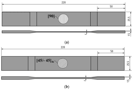
Figure 2.
CAE dimensions: (a) UD-90 specimen dimensions, and (b) SH-45 specimen dimensions; recreated according to [81].
The specimens in the first set UD-90 were designed according to the ASTM-D3039 [92] standard as transversely reinforced, unidirectionally reinforced laminates with an LSS equal to , while for the second set SH-45, according to the ASTM-D3518 [93] standard, they were designed as multidirectionally reinforced laminates with an LSS equal to which resolves the uniaxially applied tensile loads into in-plane shear loads; the visual representation of the adopted LSS is for each specimen set presented in Figure 3.
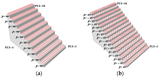
Figure 3.
(a) Layer stacking sequence for the UD-90 set, and (b) layer stacking sequence for the SH-45 set; recreated according to [81].
Both sets of specimens were tested uniaxially in quasistatic conditions with v = 0.01 mm/s using a hydraulic testing system and monitored with both contact and optical extensometers. The measurements have been taken on the opposite sides of the specimens, monitoring the strains of one surface using the epsilon-tech axial extensometer Model-3542, and the opposite one with a GOM Aramis 5M (GigE) adjustable base system with 35 mm lenses. The image resolution was 2448 × 2050 pixels, while the cameras were positioned at 560 mm from the specimen, with the distance between the cameras being equal to 265 mm, closing the angle of 26°. The sensor calibration was conducted using the software-guided protocol at 22.5 °C resulting in an average deviation of 0.048 pixels in a measuring volume of 130 × 110 mm × 90 mm. Such a measurement protocol was selected to check the consistency of the measurements through the specimen thickness and to detect excessive delamination within the gauge length. The measurements have been systematized for comparison with the RVE results and they are presented in the following chapter.
3. Results
The results are given as the microstructural observations and macroscopic experimental results, following by design of the RVEs and numerical analysis.
3.1. Microstructural Inspection
In order to obtain the necessary input for the RVE design, the material microstructure was examined on multiple cross-sections in the y-z, x-z, and x-y planes. The cross-sections were polished and scanned using an FEI-QUANTA-250-FEG scanning electron microscope; the results are presented in Figure 4.
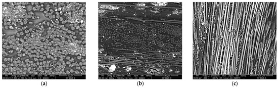
Figure 4.
CFRP SEM images: (a) y-z cross-section 1600× magnification, (b) x-z cross-section 800× magnification, and (c) x-y cross-section 800× magnification.
The acquired images were inspected and, due to the ununiform matrix background, the images were segmented based on pixel classification using Trainable WEKA segmentation machine learning algorithms in FIJI as shown in Figure 5. In the classification process, three sets of categories have been defined: the fibers, matrix, and voids with debris, each associated with the appropriate pixels. This procedure was conducted on ten randomly selected areas, while the number of included layers depended on the particular cross-section.
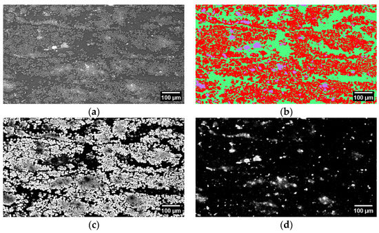
Figure 5.
CFRP laminate’s four middle unidirectional layers: (a) SEM image, (b) WEKA classification, (c) the fiber vs. matrix probability map, and (d) voids and debris probability map.
The Figure 5b shows the classified microstructure after being analyzed based on pixel recognition using the machine learning algorithms. The coloured regions define the detected phases after the training sessions and correspond to the constituents: the fibers, matrix, and voids and debris present within the analyzed material. Furthermore, the constituent’s volume ratios were identified using the colour threshold adjustment on multiple randomly selected images from each of the analyzed cross-sections, where the major contribution to the result was the images containing four middle layers in the y-z cross-section, as shown in Figure 5. Following the classification algorithm, the fibers and the ratios of the fibers, matrix, and debris and voids were identified for each of the selected images from which the average value was acquired and is presented in Table 2. However, due to the irregularity of the fiber arrangement, the local fiber volume ratio was measured on ten randomly selected 100 µm × 100 µm zones within the middle four-layer area, showing consistency with the measured average, while being inconsistent with the constituents’ volume ratios found in material agglomerations. In contrast to the volume ratios, the geometrical variable such as the fiber diameter and layer height could have been measured directly from the acquired images, and additional image refinements were not necessary for those datasets. As presented in Figure 6, the statistical analysis of the fiber diameters showed consistency with the normal distribution, while larger data discrepancies from the normal distribution could be observed in the layer height distribution which is also indicated by the Anderson–Darling value lower than 0.005.
Table 2.
Volume fraction comparison.
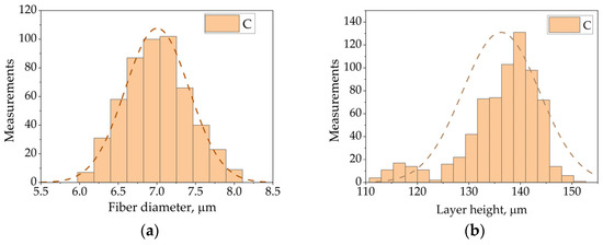
Figure 6.
(a) Carbon fiber diameter measurements, and (b) the specimen’s layer height.
The results of the statistical evaluations have been compared with the values published in the relevant literature, and the differences between the volume ratio acquired from the sample using microscopy and from the filament using pyrolysis are highlighted in Table 2. The comparison yielded consistency for the values of fiber diameters, while significant discrepancies were documented for the total and local fiber volume ratios since different machines and parameters were used in manufacturing.
Conclusively, despite the microstructural inspection having been proven valid for the identification of the constituents’ properties, it also disclosed the inconsistent repeatability of layer thickness in the AM process, which is seldom discussed, but essential for the performance of fiber-reinforced composite laminates. Despite the comparison with the relevant data in the literature yielding consistency for the values of the fiber diameters, significant discrepancies were observed for the total and local fiber volume ratios. These discrepancies could be influenced by the distinctive machines and parameters used in the manufacturing process but they were also expected since the microstructural images were extracted from the laminated specimen [13], instead of the filament presented in [85].
3.2. Experimental Acquisition of Lamina Properties
In order to identify the mechanical properties of AM continuous-fiber-reinforced composites, experimental studies on transversal and shear behavior have been conducted, following the guidelines presented in ASTM-D3039 [92] and ASTM-D3518 [93] standards. The dimensions of each specimen were assessed in multiple cross-sections within the gauge length using a digital micrometer, and the acquired values for the widths and thicknesses were averaged and are reported in Table 3. The acquired values were analyzed, showing inconsistencies in comparison with the CAE data, as presented in Figure 2, caused by the removal of the support material. Therefore, to represent the manufactured material more accurately, the measured values were adopted in the numerical analysis.
Table 3.
Dimensions of the additively manufactured specimens.
The specimens were subjected to uniaxial tensile loads and monitored with both contact and non-contact strain measurement techniques. During the experimental protocol, it was confirmed that the behavior of AM UD-90 specimens is highly influenced by the matrix response and also the fact that these specimens exhibit inferior mechanical properties in comparison to their injection-moulded counterparts [86]. The material bonding defects influenced by the fiber/matrix interface and the raster-induced defects of the additive manufacturing process act as stress concentrators which can be observed in Figure 7 as localized strains between the deposition paths. Consequently, these effects diminish the strength and stiffness of the AM materials, and due to their stochastic nature, they cause material inconsistencies, which is also confirmed by the scatter in the experimental data, and thus had to be considered in material modelling.
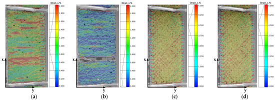
Figure 7.
DIC images of the 50 mm gauge length during the experimental procedure: (a) UD-90 pre-failure, (b) UD-90 at failure, (c) SH-45 at 5% of shear strain, and (d) SH-45 at 5% of axial strain.
Additionally, the SH-45 specimens represent a specific case of multidirectionally reinforced laminates where the adopted LSS induces multiaxial in-plane shear stress during uniaxial tension, while, similar to the case of UD-90, multiple strain localizations can be observed, as shown in Figure 7. In contrast to the UD-90 case, the SH-45 specimens demonstrated more consistent results up to 2% of shear strain, which is followed by an increase in data scatter up to 5% of shear strain. The anticipated ductile behavior for the SH-45 specimens resolves in the fiber rearrangement phenomenon which can lead to 25% of strain before failure. Since these large strains are not applicable in composite structures, the ASTM-D3518 standard [93] recommends limiting the observations of the experimental results at 5% of shear strain, in case the failure does not occur before. The shear strength in SH-45 specimens was also acquired according to the ASTM standard as the intersection between the shear stress–strain curve and the 0.2% offset of its shear modulus. The experimentally acquired data were systematized and prepared for comparison with the numerical results for each of the RVEs.
3.3. RVE Design
According to the acquired microscopic constituents’ properties, three sets of RVE models have been developed as presented in Figure 8, where RVE-1 represents a unit cell containing only one central fiber, while both RVE-2 and RVE-3 contain another fiber which is divided into four quarters placed in the RVE corners to ensure better model predictions using a smaller RVE. Furthermore, to account for the material bonding deficiencies, both the fiber/matrix and the raster-induced bonding inconsistencies have to be accounted for. However, since the scale of raster-induced defects exceeded the minimal RVE dimensions, both the matrix/fiber and the deposition contact deficiencies have been introduced together at the fiber/matrix interface as a distinctive subdomain.
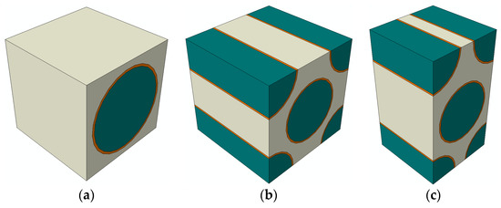
Figure 8.
(a) Single-fiber unit cell (RVE-1), (b) RVE with rectangular fiber placement (RVE-2), and (c) RVE with hexagonal fiber placement (RVE-3).
In order to check the significance of the discretization on the numerical results, a mesh sensitivity analysis was conducted on the RVE-3 case. The models were meshed using hexahedral elements (C3D8T) with characteristic lengths of , , , and , resulting in 1,115,403, 60,860, 53,876, and 33,781 elements, respectively, returning consistent results within the elastic region, while deviating from the average values for the post-yielding region in the case of , as presented in Figure 9.
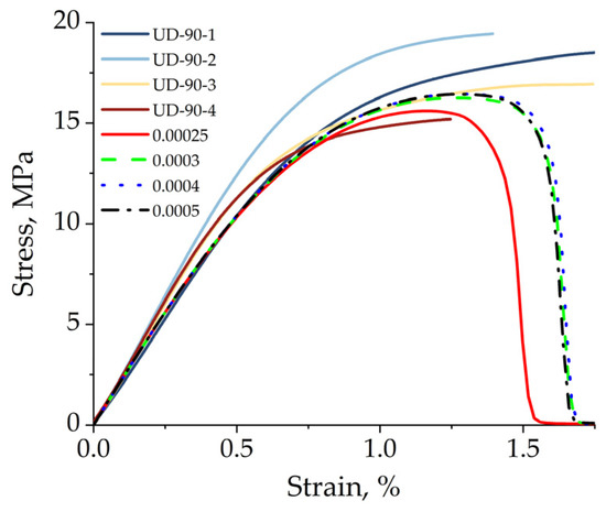
Figure 9.
Comparison between the experimental results and the RVE-3 response for characteristic element length in the range from to .
Since the presented discrepancies were less significant than the scatter within the experimental dataset, the characteristic element length of was adopted for all of the RVE cases. With the mesh size adopted, and the domains discretized, an automatized procedure [31] was adopted for enforcing the periodic boundary conditions for transverse and in-plane shear cases. In order to include the failure analysis of heterogenic materials, the procedure was modified to use the phase-field model subroutines presented in [46,80]. The necessary mechanical properties for the fiber and matrix materials were adopted from the literature, while the properties for the interface were fitted according to the experimental results. The RVEs were analyzed in the ABAQUS CAE environment, with them reaching convergence in each tested case, and the results are compared with the experimentally acquired data as presented in Figure 10, thus showing consistency for the transverse case and deviations from the experiments in the in-plane shear.
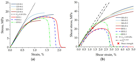
Figure 10.
Comparison between the experimental and the numerical results: (a) transversally loaded unidirectionally reinforced case, and (b) the in-plane shear case.
According to the data presented in Figure 10, there is a consistency between the modelled behaviors for the transverse tensile cases regardless of the RVE type. Furthermore, the model predictions correspond to the experimentally acquired data returning values within the scatter range. However, when subjected to in-plane shear loads, the RVE-1 and RVE-2 diverge from both the experimental results and the results acquired for the RVE-3, underestimating the shear strength and modulus, which in contrast are overestimated by the RVE-3 response. Furthermore, the resulting contour plots of the damage index are presented in Figure 11, thus supporting the interfiber damage initiation.
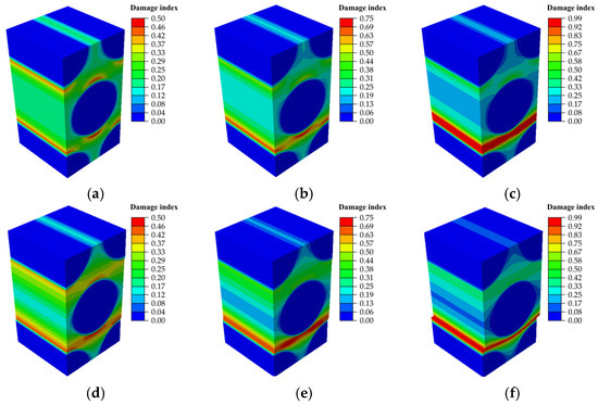
Figure 11.
Damage evolution in the transverse tensile and shear cases: (a) damage index of 0.5 in transverse tension, (b) damage index of 0.75 in transverse tension, (c) failure in transverse tension, (d) damage index of 0.5 in shear, (e) damage index of 0.75 in shear, and (f) failure in shear.
As shown in Figure 11, both RVEs subjected to transverse tensile and shear loads manifest a damage initiation at the fiber/matrix interface, which is then propagated in the matrix region, resulting in fracture. Since the fibers within the RVEs are evenly distributed by the assumption of the hexagonal array, the crack path is significantly influenced by their placements. Therefore, to investigate the crack path evolution, a randomly distributed fiber array should be adopted in further studies. All things considered, it has to be emphasized that despite the transverse micromechanical behavior being well represented, the in-plane shear cases do not follow the experimental results after 1% of shear strain and predict a complete loss of bearing capabilities after exceeding the shear strength calculated according to the ASTM guidelines, which is not the case in these laminates. Therefore, different techniques for the experimental identification and modelling of shear behavior in AM-fiber-reinforced composite materials should be considered.
4. Discussion
In order to predict the behavior of additively manufactured composite materials based on the material microstructural parameters and the constituents’ arrangements, a micromechanical modelling approach based on the representative volume element has been proposed in this work. The microscopic analysis was conducted on the representative (25 × 25 mm) cross-ply specimens through multiple cross-sections. Despite acquiring a lot of information on the material microstructure which was validated with the relevant data from the literature and then implemented in the RVE design, it was not possible to recognize any of the deposition paths in either of the cross-sections. This could be caused by the fact that the small specimen size, which is manufactured faster than the previously deposited layer, could have been completely cooled, resulting in a more homogenous microstructure without the characteristic triangular void patterns found in large-scale prints. Therefore, a scale-oriented microstructural inspection should be considered in further studies to address this issue. Furthermore, the 2D microscopic inspection in multiple cross-sections did not offer a complete insight into the materials’ microstructure. The reference coordinate system, the printing direction, and misalignments were difficult to establish without assumptions. Therefore, a µCT approach should be considered in the future both for the microstructure and the inspection of failure mechanisms.
In this study, the RVEs were designed assuming various geometrical fiber arrangements with consideration given to the measured fiber volume ratio, while keeping the RVE surfaces symmetrical to enable periodic mesh generation and the implementation of the periodic boundary conditions. Such RVEs fulfill both the geometrical and material periodicity conditions; hence, the fibers complete each other if RVEs’ segments are arranged together. However, the geometrical arrangement in these RVEs does not reflect the proper nature of the fiber arrangement found in these materials. Therefore, a statistically random fiber distribution or an input from the µCT scan should be considered in future studies. Three distinctive cases of RVEs were developed in the Abaqus CAE environment based on the results from microscopic inspections. The analysis was conducted using the phase-field fracture model available as an open-source UMAT subroutine, where the phase-field balance equation was related to the heat transfer equation readily available in the Abaqus CAE environment, hence avoiding the necessity for a dedicated UEL. This ensured the adoption of standard elements and features available in Abaqus and therefore the application of automatized procedures for enforcing the periodic boundary conditions for transversal and in-plane shear cases. In this analysis, the linear elastic constituents’ behavior was assumed, while the fracture properties were calculated according to the available properties for similar materials. Thus, for better insight into the microstructural behavior, these properties should be measured.
In order to acquire the transversal tensile and in-plane shear mechanical properties of AM CFRP composites, macroscopic evaluations were conducted on unidirectional, transversely reinforced UD-90 and multidirectionally reinforced SH-45 laminates, respectively. Both cases were tested uniaxially, where for SH-45, the adopted LSS resolved the uniaxial tensile stresses into in-plane shear. As anticipated, the transverse behavior was confirmed to be dominated by the matrix’s mechanical properties; however, the overall material response was inferior to that of the injection-moulded counterparts found in the literature, thus it was attributed to the fiber/matrix interface and the raster-induced defects of the additive manufacturing process. These effects act as stress concentrators and reduce the strength and stiffness of the AM materials, which was also confirmed in the scattering of the experimentally acquired data. These effects were also documented in the SH-45 specimens, which showed 2% divergence from the average before reaching 5% of shear strain. Therefore, both the fiber/matrix and the raster-induced bonding inconsistencies had to be accounted for in the material modelling. However, as the scale of raster-induced defects exceeded the size of the adopted RVEs, both the matrix/fiber and deposition contact deficiencies were introduced uniformly at the fiber/matrix interface. Since this approach is not physically consistent, yet based on an assumption, a multiscale representation to distinguish these effects should be considered in further studies. However, the properties of the fiber/matrix interface or the material deposition contact need to be acquired experimentally.
5. Conclusions
Numerical calculations of the transverse tensile and in-plane shear micromechanical behavior of AM CFRP materials based on the material microscopic analysis and the macroscopic response were presented in this study. The procedures used in material manufacturing and preparation for microscopic inspections were discussed, the positive and the negative aspects of the adopted approach were presented, and the key features for acquiring better results in further studies have been highlighted. The RVE design based on geometrical assumptions and supported by the microstructural measurements was also discussed, where many benefits of using µCT over microscopy have been presented. Furthermore, the presented microstructural analysis is based on the proposed analogy between phase-field fracture and the thermal conductivity differential equations since it supports the ABAQUS built-in features, thus enabling the development and analysis of the periodic RVEs using the phase-field fracture theory. This approach simplified the domain divisions based on the various materials and their interfaces, as well as the load application and finally the visualization of the acquired result. Furthermore, both the data scatter and the DIC images confirmed that the inconsistencies in AM CFRP composites are caused in the contact zones of the deposited material. However, since the scale of these deficiencies exceeded the size of the proposed RVEs, the effects were introduced together with the fiber/matrix influence at the constituents’ interface. The negative aspects of this approach were discussed, and a multiscale approach with experimentally acquired interface properties was proposed for further study.
All things considered, this study confirmed consistency between the experimental results and the numerical prediction using the phase-field fracture approach for the transverse tensile behavior of AM CFRP composites. The numerical results were independent of the RVE type, returning values within the range of the experimental scatter. However, when analyzing the in-plane shear behavior, RVE-1 and RVE-2 revealed divergence from both the experimental results and the results acquired for the RVE-3, thus underestimating the shear strength and modulus of the tested materials. In contrast, RVE-3 overestimated the mechanical properties in the case of in-plane shear. It was shown that despite the transverse micromechanical behavior being well characterized using this phase-field modelling approach, the in-plane shear cases do not follow the experimental results after 1% of shear strain. Furthermore, after exceeding the shear strength calculated according to the ASTM guidelines, the model predicts a complete specimen failure which does not occur in the experiments. Therefore, different techniques for experimental identification and modelling of shear behavior in AM-fiber-reinforced composite materials should be considered in future work.
Author Contributions
M.G.: writing–original draft, visualization, software, methodology, investigation, and formal analysis. D.L.: writing—review and editing, supervision, project administration, and funding acquisition. M.F.: writing—review and editing, supervision, project administration, and funding acquisition. A.Ž.: writing—review and editing, validation, resources, methodology, and investigation. All authors have read and agreed to the published version of the manuscript.
Funding
The research presented in this paper was made possible by the financial support of Croatian Science Foundation (project No. IP-2019-04-8615) and (project No. IP-2019-04-3607), and the University of Rijeka (uniri-tehnic-18-139) and (uniri-tehnic-18-34).
Data Availability Statement
Data will be available on request.
Acknowledgments
Special thanks to IB-CADDY d.o.o., the Institute of Metals and Technology (IMT) in Ljubljana, Slovenia, and the Center for Advanced Computing and Modelling (CNRM) at the University of Rijeka for their technical assistance in the manufacturing and experimental procedures.
Reprints
Figure 7 was reprinted as detail from Additive Manufacturing, 56, M. Gljušćić, M. Franulović, D. Lanc, A. Žerovnik, Representative volume element for microscale analysis of additively manufactured composites/ Results and discussion, Page 9., Copyright (2022), with permission from Elsevier.
Conflicts of Interest
The authors declare that they have no known competing financial interests or personal relationships that could have appeared to have influence the work reported in this paper.
Appendix A
A formulation of the phase-field fracture theory reproduced according to [46,80,89].
The strain tensor is calculated based on the displacement field vector u, under the assumption of small strain sand isothermal conditions, as shown in Equation (A1) [46,80,89].
The degree of damage is described with a continuous phase field scalar which takes values between zero and one, regarded as undamaged and fully damaged material, respectively [46,80,89]. The smeared crack approach is used to represent the discrete nature of the cracks, and it is regulated by a length scale variable , under the approximation of the fracture energy over a discontinuous surface ; where is the crack surface density functional, while the material toughness is given by , as shown in Equation (A2) [46,80,89].
Under the assumption that the phase field depends only on the solution of the displacement problem, the external traction forces are not included in the calculation of the principle of virtual work, as shown in Equation (A3).
In the Equation (A3), the Cauchy stress tensor is represented by , which is work-conjugate to the strains represented by . The traction T is defined for the outward unit normal n at boundary , and it is work-conjugate to the displacements u [46,80,89]. The work-conjugate to the phase field is given by , while is the micro-stress vector, a work-conjugate to the , as the virtual quantity is given by [46,80,89].
In the material domain , the local force balance is calculated according to the expressions given in Equation (A4), assuming and boundary conditions on [46,80,89].
The generalized expression for the potential energy is presented in Equation (A5) [46,80,89], where the elastic strain and the facture energy densities are given by and , respectively, and represents the degradation function [46,80,89].
By adopting the degradation function and assuming the criteria presented in Equation (A6) [46,80,89], the value of the potential energy is decreased with the increase in damage in the material [46,80,89].
According to the presented assumptions, the expression for the fracture energy density is given in Equation (A7) [46,80,89], where the length scale of the phase field is represented by , is a scaling constant, and is a geometric crack function, as the damage growth is realized with the stored elastic energy which is characterized by the elastic strain energy density in the undamaged state [46,80,89].
In order to prevent the crack development in compression, the fracture driving force is decomposed to the active and inactive parts, represented by and , respectively [46,80,89], which leads to the definition of the elastic strain energy density presented in Equation (A8) [46,80,89].
The damage irreversibility is represented as , and it is achieved using the history field variable which fulfills the Karush–Kuhn–Tucker (KKT) conditions presented in Equation (A8) [46,80,89].
This leads to a history field definition for a specific time referred to as over a total time given by , as shown in Equation (A10), and the reformulation of the potential energy is shown in Equation (A11) [46,80,89].
Scalar micro-stress scalar and the micro-stress vector are calculated according to the expressions presented in Equations (A12) and (A13), respectively [46,80,89], which were incorporated into Equation (A14), and this leads to the phase field evolution law presented in Equation (A15) [46,80,89].
The heat transfer analogy is based on the evolution of the temperature field T in a specific time t as shown in Equation (A15) [46,80,89], where the thermal conductivity of the material is represented by k, the specific heat is represented by , and the density is represented by [46,80,89].
If steady-state conditions are assumed, the reduces to zero, and the expression is simplified as shown in Equation (A16) [46,80,89].
In order to correspond with Equation (A16), the phase field evolution law presented in Equation (A14) can be rearranged as shown in Equation (A17) [46,80,89].
According to [46,80,89], this analogy can be adopted considering the equivalence between the temperature and the phase field assuming the thermal conductivity is equal to one and by defining the heat flux according to the internal heat generation, as shown in Equation (A18), while in order to compute the Jacobian matrix, the heat flux rate of change is defined according to Equation (A19).
Since the total potential energy is minimized according to the displacement field u and phase field Φ, while Φ is being solved at the finite element nodes such as a damage variable at the finite element node instead of at the integration point as in the case of local damage models, the calculation would require the user-defined element (UEL) before the implementation of the user-defined material model (UMAT). However, since this approach uses the heat transfer analogy, the UMAT subroutine can be run without the necessity for the user-defined element.
Steps for the implementation of the subroutine [89]:
- Define the user material with five material properties including the Young’s modulus , Poisson’s ratio , phase field length scale , fracture toughness , and the tensile strength which is applicable for the phase field cohesive zone models, while otherwise neglected
- Set a solution-dependent state variable (SDV)
- Define the material conductivity equal to one
- State the analysis step as coupled temperature-displacement with steady-state or transient options, a constant increment size, a separated solution technique, and symmetric equation solver matrix storage
- Change the values of the solution controls parameters to 5000, to avoid convergence problems due to large number of iterations
- Define the initial temperature condition equal to zero to describe the undamaged material in the initial step
- Adopt the element type as coupled temperature–displacement
References
- Alghamdi, S.S.; John, S.; Choudhury, N.R.; Dutta, N.K. Additive Manufacturing of Polymer Materials: Progress, Promise and Challenges. Polymers 2021, 13, 753. [Google Scholar] [CrossRef]
- Ferreira, I.; Machado, M.; Alves, F.; Torres Marques, A. A Review on Fibre Reinforced Composite Printing via FFF. Rapid Prototyp. J. 2019, 25, 972–988. [Google Scholar] [CrossRef]
- Ngo, T.D.; Kashani, A.; Imbalzano, G.; Nguyen, K.T.Q.; Hui, D. Additive Manufacturing (3D Printing): A Review of Materials, Methods, Applications and Challenges. Compos. Part B 2018, 143, 172–196. [Google Scholar] [CrossRef]
- van de Werken, N.; Tekinalp, H.; Khanbolouki, P.; Ozcan, S.; Williams, A.; Tehrani, M. Additively Manufactured Carbon Fiber-Reinforced Composites: State of the Art and Perspective. Addit. Manuf. 2020, 31, 100962. [Google Scholar] [CrossRef]
- van de Werken, N. Additively Manufactured Continuous Carbon Fiber Thermoplastic Composites for High-Performance Applications. Doctoral Dissertation, The University of New Mexico, Albuquerque, NM, USA, 2019. [Google Scholar]
- Karaş, B.; Smith, P.J.; Fairclough, J.P.A.; Mumtaz, K. Additive Manufacturing of High Density Carbon Fibre Reinforced Polymer Composites. Addit. Manuf. 2022, 58, 103044. [Google Scholar] [CrossRef]
- Rengier, F.; Mehndiratta, A.; Von Tengg-Kobligk, H.; Zechmann, C.M.; Unterhinninghofen, R.; Kauczor, H.U.; Giesel, F.L. 3D Printing Based on Imaging Data: Review of Medical Applications. Int. J. Comput. Assist. Radiol. Surg. 2010, 5, 335–341. [Google Scholar] [CrossRef]
- Schubert, C.; Van Langeveld, M.C.; Donoso, L.A. Innovations in 3D Printing: A 3D Overview from Optics to Organs. Br. J. Ophthalmol. 2014, 98, 159–161. [Google Scholar] [CrossRef]
- Diegel, O.; Nordin, A.; Motte, D. Additive Manufacturing Technologies; Springer: Berlin/Heidelberg, Germany, 2019; ISBN 9781493921126. [Google Scholar]
- Abazari, S.; Shamsipur, A.; Bakhsheshi-Rad, H.R.; Ismail, A.F. Carbon Nanotubes (CNTs)-Reinforced Magnesium-Based Matrix Composites: A Comprehensive Review. J. Higher Educ. 2020, 13, 38. [Google Scholar] [CrossRef]
- Abazari, S.; Shamsipur, A.; Bakhsheshi-Rad, H.R.; Ramakrishna, S.; Berto, F. Graphene Family Nanomaterial Reinforced Magnesium-Based Matrix Composites for Biomedical Application: A Comprehensive Review. Metals 2020, 10, 1002. [Google Scholar] [CrossRef]
- Monfared, V.; Bakhsheshi-Rad, H.R.; Ramakrishna, S.; Razzaghi, M.; Berto, F. A Brief Review on Additive Manufacturing of Polymeric Composites and Nanocomposites. Micromachines 2021, 12, 24. [Google Scholar] [CrossRef]
- Gljušćić, M.; Franulović, M.; Lanc, D.; Žerovnik, A. Representative Volume Element for Microscale Analysis of Additively Manufactured Composites. Addit. Manuf. 2022, 56, 102902. [Google Scholar] [CrossRef]
- Gljušćić, M.; Franulović, M.; Žužek, B.; Žerovnik, A. Experimental Validation of Progressive Damage Modeling in Additively Manufactured Continuous Fiber Composites. Compos. Struct. 2022, 295, 115869. [Google Scholar] [CrossRef]
- Iragi, M.; Pascual-González, C.; Esnaola, A.; Lopes, C.S.; Aretxabaleta, L. Ply and Interlaminar Behaviours of 3D Printed Continuous Carbon Fibre-Reinforced Thermoplastic Laminates; Effects of Processing Conditions and Microstructure. Addit. Manuf. 2019, 30, 100884. [Google Scholar] [CrossRef]
- Carlota, V. Essentium’s Latest Survey: What Is the Future of Industrial 3D Printing? Available online: https://www.3dnatives.com/en/essentium-190320195/ (accessed on 15 October 2022).
- Gide, K.M.; Islam, S.; Bagheri, Z.S. Polymer-Based Materials Built with Additive Manufacturing Methods for Orthopedic Applications: A Review. J. Compos. Sci. 2022, 6, 262. [Google Scholar] [CrossRef]
- Deeba, F.; Shrivastava, K.; Bafna, M.; Jain, A. Tuning of Dielectric Properties of Polymers by Composite Formation: The Effect of Inorganic Fillers Addition. J. Compos. Sci. 2022, 6, 355. [Google Scholar] [CrossRef]
- Tran, C.C.; Nguyen, Q.K. An Efficient Method to Determine the Thermal Behavior of Composite Material with Loading High Thermal Conductivity Fillers. J. Compos. Sci. 2022, 6, 214. [Google Scholar] [CrossRef]
- Kabir, S.M.F.; Mathur, K.; Seyam, A.F.M. Maximizing the Performance of 3d Printed Fiber-Reinforced Composites. J. Compos. Sci. 2021, 5, 136. [Google Scholar] [CrossRef]
- Melenka, G.W.; Cheung, B.K.O.; Schofield, J.S.; Dawson, M.R.; Carey, J.P. Evaluation and Prediction of the Tensile Properties of Continuous Fiber-Reinforced 3D Printed Structures. Compos. Struct. 2016, 153, 866–875. [Google Scholar] [CrossRef]
- He, Q.; Wang, H.; Fu, K.; Ye, L. 3D Printed Continuous CF/PA6 Composites: Effect of Microscopic Voids on Mechanical Performance. Compos. Sci. Technol. 2020, 191, 108077. [Google Scholar] [CrossRef]
- Baechle-Clayton, M.; Loos, E.; Taheri, M.; Taheri, H. Failures and Flaws in Fused Deposition Modeling (FDM) Additively Manufactured Polymers and Composites. J. Compos. Sci. 2022, 6, 202. [Google Scholar] [CrossRef]
- Suquet, P. Continuum Micromechanics; Kaliszky, S., Sayir, M., Schneider, W., Bianchi, G., Tasso, C., Eds.; Springer: Berlin/Heidelberg, Germany, 1997; ISBN 9783211829028. [Google Scholar]
- Michel, J.C.; Moulinec, H.; Suquet, P. Effective Properties of Composite Materials with Periodic Microstructure: A Computational Approach. Comput. Methods Appl. Mech. Eng. 1999, 172, 109–143. [Google Scholar] [CrossRef]
- Rémond, Y.; Ahzi, S. Applied RVE Reconstruction and Homogenization of Heterogeneous Materials; John Wiley & Sons: Hoboken, NJ, USA, 2016; ISBN 9781848219014. [Google Scholar]
- Soutis, C.; Beaumont, P.W.R. Multi-Scale Modelling of Composite Material Systems: The Art of Predictive Damage Modelling; Woodhead Publishing Limited: Sawston, UK; CRC Press LLC: Boca Raton, FL, USA, 2005; Volume 3, ISBN 978-1-85573-936-9. [Google Scholar]
- Múgica, J.I.; Lopes, C.S.; Naya, F.; Herráez, M.; Martínez, V.; González, C. Multiscale Modelling of Thermoplastic Woven Fabric Composites: From Micromechanics to Mesomechanics. Compos. Struct. 2019, 228, 111340. [Google Scholar] [CrossRef]
- Riaño, L.; Joliff, Y. An ABAQUSTM Plug-in for the Geometry Generation of Representative Volume Elements with Randomly Distributed Fibers and Interphases. Compos. Struct. 2019, 209, 644–651. [Google Scholar] [CrossRef]
- Raju, B.; Hiremath, S.R.; Roy Mahapatra, D. A Review of Micromechanics Based Models for Effective Elastic Properties of Reinforced Polymer Matrix Composites. Compos. Struct. 2018, 204, 607–619. [Google Scholar] [CrossRef]
- Omairey, S.L.; Dunning, P.D.; Sriramula, S. Development of an ABAQUS Plugin Tool for Periodic RVE Homogenisation. Eng. Comput. 2019, 35, 567–577. [Google Scholar] [CrossRef]
- Akpoyomare, A.I.; Okereke, M.I.; Bingley, M.S. Virtual Testing of Composites: Imposing Periodic Boundary Conditions on General Finite Element Meshes. Compos. Struct. 2017, 160, 983–994. [Google Scholar] [CrossRef]
- Okereke, M.I.; Akpoyomare, A.I. A Virtual Framework for Prediction of Full-Field Elastic Response of Unidirectional Composites. Comput. Mater. Sci. 2013, 70, 82–99. [Google Scholar] [CrossRef]
- Kempesis, D.; Iannucci, L.; Ramesh, K.T.; Del Rosso, S.; Curtis, P.T.; Pope, D.; Duke, P.W. Micromechanical Analysis of High Fibre Volume Fraction Polymeric Laminates Using Micrograph-Based Representative Volume Element Models. Compos. Sci. Technol. 2022, 229, 109680. [Google Scholar] [CrossRef]
- Schindelin, J.; Arganda-Carreras, I.; Frise, E.; Kaynig, V.; Longair, M.; Pietzsch, T.; Preibisch, S.; Rueden, C.; Saalfeld, S.; Schmid, B.; et al. Fiji: An Open-Source Platform for Biological-Image Analysis. Nat. Methods 2012, 9, 676–682. [Google Scholar] [CrossRef]
- Breite, C.; Melnikov, A.; Turon, A.; de Morais, A.B.; Le Bourlot, C.; Maire, E.; Schöberl, E.; Otero, F.; Mesquita, F.; Sinclair, I.; et al. Detailed Experimental Validation and Benchmarking of Six Models for Longitudinal Tensile Failure of Unidirectional Composites. Compos. Struct. 2022, 279, 114828. [Google Scholar] [CrossRef]
- Liu, Y.; Straumit, I.; Vasiukov, D.; Lomov, S.V.; Panier, S. Multi-Scale Material Model for 3D Composite Using Micro CT Images Geometry Reconstruction. In Proceedings of the 7th European Conference on Composite Materials (ECCM), Munich, Germany, 26–30 June 2016. [Google Scholar]
- Straumit, I.; Lomov, S.V.; Wevers, M. Quantification of the Internal Structure and Automatic Generation of Voxel Models of Textile Composites from X-Ray Computed Tomography Data. Compos. Part A Appl. Sci. Manuf. 2015, 69, 150–158. [Google Scholar] [CrossRef]
- Dean, A.; Asur Vijaya Kumar, P.K.; Reinoso, J.; Gerendt, C.; Paggi, M.; Mahdi, E.; Rolfes, R. A Multi Phase-Field Fracture Model for Long Fiber Reinforced Composites Based on the Puck Theory of Failure. Compos. Struct. 2020, 251, 112446. [Google Scholar] [CrossRef]
- Guillén-Hernández, T.; García, I.G.; Reinoso, J.; Paggi, M. A Micromechanical Analysis of Inter-Fiber Failure in Long Reinforced Composites Based on the Phase Field Approach of Fracture Combined with the Cohesive Zone Model. Int. J. Fract. 2019, 220, 181–203. [Google Scholar] [CrossRef]
- Tan, W.; Martínez-Pañeda, E. Phase Field Fracture Predictions of Microscopic Bridging Behaviour of Composite Materials. Compos. Struct. 2022, 286, 115242. [Google Scholar] [CrossRef]
- Griffith, A.A., VI. The phenomena of rupture and flow in solids. Philos. Trans. R. Soc. Lond. 1921, 221, 163–198. [Google Scholar] [CrossRef]
- Biner, S.B. Programming Phase-Field Modeling; Springer: Cham, Switzerland, 2017; ISBN 9783319411965. [Google Scholar]
- Francfort, G.A.; Marigo, J.J. Revisiting Brittle Fracture as an Energy Minimization Problem. J. Mech. Phys. Solids 1998, 46, 1319–1342. [Google Scholar] [CrossRef]
- Bourdin, B.; Francfort, G.A.; Marigo, J. Numerical Experiments in Revisited Brittle Fracture. J. Mech. Phys. Solids 2000, 48, 797–826. [Google Scholar] [CrossRef]
- Navidtehrani, Y.; Betegón, C.; Martínez-Pañeda, E. A Unified Abaqus Implementation of the Phase Field Fracture Method Using Only a User Material Subroutine. Materials 2021, 14, 1913. [Google Scholar] [CrossRef]
- Tourret, D.; Liu, H.; LLorca, J. Phase-Field Modeling of Microstructure Evolution: Recent Applications, Perspectives and Challenges. Prog. Mater. Sci. 2022, 123, 100810. [Google Scholar] [CrossRef]
- Egger, A.; Pillai, U.; Agathos, K.; Kakouris, E.; Chatzi, E.; Aschroft, I.A.; Triantafyllou, S.P. Discrete and Phase Field Methods for Linear Elastic Fracture Mechanics: A Comparative Study and State-of-the-Art Review. Appl. Sci 2019, 9, 2436. [Google Scholar] [CrossRef]
- Wu, J.; Huang, Y. Comprehensive Implementations of Phase-Field Damage Models in Abaqus. Theor. Appl. Fract. Mech. 2020, 106, 102440. [Google Scholar] [CrossRef]
- Simoes, M.; Martínez-pañeda, E. Phase Field Modelling of Fracture and Fatigue in Shape Memory Alloys. Comput. Methods Appl. Mech. Eng. 2021, 373, 113504. [Google Scholar] [CrossRef]
- Natarajan, S.; Annabattula, R.K.; Martínez-pañeda, E. Phase Field Modelling of Crack Propagation in Functionally Graded Materials. Compos. Part B 2019, 169, 239–248. [Google Scholar] [CrossRef]
- Asur Vijaya Kumar, P.K.; Dean, A.; Reinoso, J.; Lenarda, P.; Paggi, M. Phase Field Modeling of Fracture in Functionally Graded Materials: Γ-Convergence and Mechanical Insight on the Effect of Grading. Thin-Walled Struct. 2021, 159, 107234. [Google Scholar] [CrossRef]
- Miehe, C.; Schänzel, L. Phase Field Modeling of Fracture in Rubbery Polymers. Part I: Finite Elasticity Coupled with Brittle Failure. J. Mech. Phys. Solids 2014, 65, 93–113. [Google Scholar] [CrossRef]
- Loew, P.J.; Peters, B.; Beex, L.A.A. Rate-Dependent Phase-Field Damage Modeling of Rubber and Its Experimental Parameter Identification. J. Mech. Phys. Solids 2019, 127, 266–294. [Google Scholar] [CrossRef]
- Zhou, S.; Zhuang, X.; Rabczuk, T. Phase Field Modeling of Brittle Compressive-Shear Fractures in Rock-like Materials: A New Driving Force and a Hybrid Formulation. Comput. Methods Appl. Mech. Eng. 2019, 355, 729–752. [Google Scholar] [CrossRef]
- Schuler, L.; Ilgen, A.G.; Newell, P. Chemo-Mechanical Phase-Field Modeling of Dissolution-Assisted Fracture. Comput. Methods Appl. Mech. Eng. 2020, 362, 112838. [Google Scholar] [CrossRef]
- Kristensen, P.K.; Martínez-pañeda, E.; Engineering, M.; Lyngby, D.-K. Phase Field Fracture Modelling Using Quasi-Newton Methods and a New Adaptive Step Scheme. Theor. Appl. Fract. Mech. 2020, 107, 102446. [Google Scholar] [CrossRef]
- Abdollahi, A.; Arias, I. Phase-Field Modeling of Crack Propagation in Piezoelectric and Ferroelectric Materials with Different Electromechanical Crack Conditions. J. Mech. Phys. Solids 2012, 60, 2100–2126. [Google Scholar] [CrossRef]
- Pillai, U. Damage Modelling in Fibre-Reinforced Composite Laminates Using Phase Field Approach. Doctoral Dissertation, University of Nottingham, Nottingham, UK, 2021. [Google Scholar]
- Quintanas-corominas, A.; Reinoso, J.; Casoni, E.; Turon, A.; Mayugo, J.A. A Phase Field Approach to Simulate Intralaminar and Translaminar Fracture in Long Fiber Composite Materials. Compos. Struct. 2019, 220, 899–911. [Google Scholar] [CrossRef]
- Ahmadi, M. A Hybrid Phase Field Model for Fracture Induced by Lithium Diffusion in Electrode Particles of Li-Ion Batteries. Comput. Mater. Sci. 2020, 184, 109879. [Google Scholar] [CrossRef]
- Nguyen, T.T.; Yvonnet, J.; Zhu, Q.Z.; Bornert, M.; Chateau, C. A Phase Field Method to Simulate Crack Nucleation and Propagation in Strongly Heterogeneous Materials from Direct Imaging of Their Microstructure. Eng. Fract. Mech. 2015, 139, 18–39. [Google Scholar] [CrossRef]
- Goswami, S.; Anitescu, C.; Rabczuk, T. Adaptive Phase Field Analysis with Dual Hierarchical Meshes for Brittle Fracture. Eng. Fract. Mech. 2019, 218, 106608. [Google Scholar] [CrossRef]
- Goswami, S.; Anitescu, C.; Rabczuk, T. Adaptive Fourth-Order Phase Field Analysis Using Deep Energy Minimization. Theor. Appl. Fract. Mech. 2020, 107, 102527. [Google Scholar] [CrossRef]
- Huynh, G.D.; Zhuang, X.; Nguyen-Xuan, H. Implementation Aspects of a Phase-Field Approach for Brittle Fracture. Front. Struct. Civ. Eng. 2019, 13, 417–428. [Google Scholar] [CrossRef]
- Msekh, M.A.; Sargado, J.M.; Jamshidian, M.; Areias, P.M.; Rabczuk, T. Abaqus Implementation of Phase-Field Model for Brittle Fracture. Comput. Mater. Sci. 2015, 96, 472–484. [Google Scholar] [CrossRef]
- Liu, G.; Li, Q.; Msekh, M.A.; Zuo, Z. Abaqus Implementation of Monolithic and Staggered Schemes for Quasi-Static and Dynamic Fracture Phase-Field Model. Comput. Mater. Sci. 2016, 121, 35–47. [Google Scholar] [CrossRef]
- Molnár, G.; Gravouil, A. 2D and 3D Abaqus Implementation of a Robust Staggered Phase-Field Solution for Modeling Brittle Fracture. Finite Elem. Anal. Des. 2017, 130, 27–38. [Google Scholar] [CrossRef]
- Pillai, U.; Heider, Y.; Markert, B. A Diffusive Dynamic Brittle Fracture Model for Heterogeneous Solids and Porous Materials with Implementation Using a User-Element Subroutine. Comput. Mater. Sci. 2018, 153, 36–47. [Google Scholar] [CrossRef]
- Bhowmick, S.; Liu, G.R. A Phase-Field Modeling for Brittle Fracture and Crack Propagation Based on the Cell-Based Smoothed Finite Element Method. Eng. Fract. Mech. 2018, 204, 369–387. [Google Scholar] [CrossRef]
- Seleš, K.; Lesičar, T.; Tonković, Z.; Sorić, J. A Residual Control Staggered Solution Scheme for the Phase-Field Modeling of Brittle Fracture. Eng. Fract. Mech. 2019, 205, 370–386. [Google Scholar] [CrossRef]
- Zhou, S.; Rabczuk, T.; Zhuang, X. Phase Field Modeling of Quasi-Static and Dynamic Crack Propagation: COMSOL Implementation and Case Studies. Adv. Eng. Softw. 2018, 122, 31–49. [Google Scholar] [CrossRef]
- Pham, K.; Amor, H.; Marigo, J.J.; Maurini, C. Gradient Damage Models and Their Use to Approximate Brittle Fracture. Int. J. Damage Mech. 2011, 20, 618–652. [Google Scholar] [CrossRef]
- Wu, J.Y. A Unified Phase-Field Theory for the Mechanics of Damage and Quasi-Brittle Failure. J. Mech. Phys. Solids 2017, 103, 72–99. [Google Scholar] [CrossRef]
- Wu, J.Y. A Geometrically Regularized Gradient-Damage Model with Energetic Equivalence. Comput. Methods Appl. Mech. Eng. 2018, 328, 612–637. [Google Scholar] [CrossRef]
- Wu, J.Y.; Nguyen, V.P. A Length Scale Insensitive Phase-Field Damage Model for Brittle Fracture. J. Mech. Phys. Solids 2018, 119, 20–42. [Google Scholar] [CrossRef]
- Zhang, P.; Hu, X.; Wang, X.; Yao, W. An Iteration Scheme for Phase Field Model for Cohesive Fracture and Its Implementation in Abaqus. Eng. Fract. Mech. 2018, 204, 268–287. [Google Scholar] [CrossRef]
- Miehe, C.; Hofacker, M.; Welschinger, F. A Phase Field Model for Rate-Independent Crack Propagation: Robust Algorithmic Implementation Based on Operator Splits. Comput. Methods Appl. Mech. Eng. 2010, 199, 2765–2778. [Google Scholar] [CrossRef]
- Gerasimov, T.; De Lorenzis, L. A Line Search Assisted Monolithic Approach for Phase-Field Computing of Brittle Fracture. Comput. Methods Appl. Mech. Eng. 2016, 312, 276–303. [Google Scholar] [CrossRef]
- Navidtehrani, Y.; Betegón, C.; Martínez-Pañeda, E. A Simple and Robust Abaqus Implementation of the Phase Field Fracture Method. Appl. Eng. Sci. 2021, 6, 100050. [Google Scholar] [CrossRef]
- Gljušćić, M. Multiscale Modelling of Additively Manufactured Composite Material Behaviour. Doctoral Dissertation, University of Rijeka, Rijeka, Croatia, 2022. [Google Scholar]
- Iragi, M.; Pascual-Gonzalez, C.; Esnaola, A.; Aurrekoetxea, J.; Lopes, C.S.; Aretxabaleta, L. Characterization of Elastic and Resistance Behaviours of 3D Printed Continuous Carbon Fibre Reinforced Thermoplastics. In Proceedings of the ECCM18—18th European Conference on Composite Materials, Athens, Greece, 24–28 June 2018; pp. 24–28. [Google Scholar]
- Carraro, P.A.; Quaresimin, M. A Stiffness Degradation Model for Cracked Multidirectional Laminates with Cracks in Multiple Layers. Int. J. Solids Struct. 2014, 58, 34–51. [Google Scholar] [CrossRef]
- Okereke, M.; Keates, S. Finite Element Applications: A Practical Guide to the FEM Process; Seung-Bok, C., Habinin, D., Fu, Y., Guardiola, C., Sun, J.-Q., Eds.; Springer International Publishing: Cham, Switzerland, 2018; ISBN 978-3-319-67124-6. [Google Scholar]
- Pascual-González, C.; Iragi, M.; Fernández, A.; Fernández-Blázquez, J.P.; Aretxabaleta, L.; Lopes, C.S. An Approach to Analyse the Factors behind the Micromechanical Response of 3D-Printed Composites. Compos. Part B Eng. 2020, 186, 107820. [Google Scholar] [CrossRef]
- VDI/VDE 2479; Materials for Precision Engineering; Polyamide Moulding Materials Unreinforced. VDI-Verlag GmbH: Dusseldorf, Germany, 1978; Volume 1.
- MarkForged. Material Datasheet Composites; Markforged: Watertown, MA, USA, 2018. [Google Scholar]
- Nabavi, A.; Goroshin, S.; Frost, D.L.; Barthelat, F. Mechanical Properties of Chromium–Chromium Sulfide Cermets Fabricated by Self-Propagating High-Temperature Synthesis. J. Mater. Sci. 2015, 50, 3434–3446. [Google Scholar] [CrossRef]
- Navidtehrani, Y.; Martinez-Paneda, E. A Simple yet General ABAQUS Phase Field Fracture Implementation Using a UMAT Subroutine. Eng. Sci. 2021, 6, 100050. [Google Scholar]
- Ambati, M.; Gerasimov, T.; De Lorenzis, L. A Review on Phase-Field Models of Brittle Fracture and a New Fast Hybrid Formulation. Comput. Mech. 2015, 55, 383–405. [Google Scholar] [CrossRef]
- Amor, H.; Marigo, J.J.; Maurini, C. Regularized Formulation of the Variational Brittle Fracture with Unilateral Contact: Numerical Experiments. J. Mech. Phys. Solids 2009, 57, 1209–1229. [Google Scholar] [CrossRef]
- ASTM D3039/D3039M-17; Standard Test Method for Tensile Properties of Polymer Matrix Composite Materials. ASTM International: West Conshohocken, PA, USA, 2017.
- ASTM D3518/D3518M; 18 Standard Test Method for In-Plane Shear Response of Polymer Matrix Composite Materials by Tensile Test of a +/−45° Laminate. ASTM International: West Conshohocken, PA, USA, 2001; pp. 1–7.
Disclaimer/Publisher’s Note: The statements, opinions and data contained in all publications are solely those of the individual author(s) and contributor(s) and not of MDPI and/or the editor(s). MDPI and/or the editor(s) disclaim responsibility for any injury to people or property resulting from any ideas, methods, instructions or products referred to in the content. |
© 2023 by the authors. Licensee MDPI, Basel, Switzerland. This article is an open access article distributed under the terms and conditions of the Creative Commons Attribution (CC BY) license (https://creativecommons.org/licenses/by/4.0/).