Simplified Approach for the Seismic Assessment of Existing X Shaped CBFs: Examples and Numerical Applications

Abstract

The capacity of a structure can be assessed using inelastic analyses, requiring sophisticated numerical procedures such as pushover and incremental dynamic analyses. A simplified method for the evaluation of the seismic performance of steel Concentrically Braced Frames (CBFs) to be used in everyday practice and the immediate aftermath of an earthquake has been recently proposed. This method evaluates the capacity of an existing building employing an analytical trilinear model without resorting to any non-linear analysis. The proposed methodology has been set up through a large parametric analysis, carried out on 420 frames designed according to three different approaches: the first one is the Theory of Plastic Mechanism Control (TPMC), ensuring the design of structures showing global collapse mechanisms (GCBFs), the second one is based on the Eurocode 8 design requirements (SCBFs), and the third is a non-seismic design, based on a non-seismic design (OCBFs). In this paper, some examples of the application of this simplified methodology are proposed with references to structures that are supposed to exhibit global, partial, and soft storey mechanisms.

1. Introduction

Recent seismic events have underlined the high seismic vulnerability of a large part of the built heritage and, consequently, the importance of its safeguarding [1,2,3,4,5,6,7,8,9,10,11,12,13,14,15,16,17,18,19,20,21]. With a view to a large-scale classification of the existing buildings in terms of seismic vulnerability, the definition of a simplified methodology that allows for an evaluation of the seismic performance without resorting to analyses that require high numerical complexities, such as pushover analysis and incremental dynamic analysis, plays an important role [22,23,24,25,26,27,28,29,30,31]. These procedures also do not result in seismic classification and code liability, being strongly influenced by the software used to develop them, nor the modeling of the members, which is characterized by numerous variables that are difficult to standardize [32,33,34,35].

Consequently, a completely analytical simplified model allowing us to univocally control these complexities is introduced for steel Concentrically Braced Frames (CBFs) [36].

The methodology is set up for general use. It is based on the use of elastic analysis combined with rigid plastic analysis for both CBFs and MRFs. The difference lies in the definition of some characteristic points. The capacity curve is represented through a trilinear approximation. In particular, CBFs are characterized by presenting a second elastic branch with reduced stiffness for the buckling of the compressed diagonals, whereas MRFs have a horizontal branch due to the plastic redistribution capacity typical of the structural type.

The performance-based assessment procedure is herein applied to some study cases in order to testify both the ease and speed of the application of the method. This procedure consists of identifying some characteristic points associated with target performance objectives on a trilinear simplified capacity curve [37,38]. These points correspond to different limit states.

The procedure was validated by a wide parametric analysis on 420 CBFs, designed according to three different approaches, i.e., for horizontal loads only (OCBFs), according to the provisions of Eurocode 8 (SCBFs), and in accordance with the theory of plastic mechanism control (GCBFs). The design according to three approaches was carried out to ensure a database of frames capable of covering the design philosophies of recent decades. It is known that structures designed without prescriptions aimed at controlling the collapse mechanism are used to exhibit soft storey mechanisms, unlike structures designed according to Eurocode 8, which are capable of avoiding these types of mechanisms without, however, guaranteeing the development of global collapse mechanisms, which is obtainable instead with the use of the TPMC approach. For the designed structures, pushover analyses were carried out to calibrate the proposed analytical relationships and, thus, to ensure a wide applicability of the method.

The comparison in terms of capacity and demand can be made according to two alternative approaches: the one proposed by Eurocode 8 [39] and the one proposed by Nassar and Krawinkler [40]. The former exploits the concept of the ADRS spectrum, whereas the latter has the benefit of having an easier applicability because it does not distinguish between low and high periods of vibration. In the following, the main model equations are reported and described.

2. Fundamental Equations of the Trilinear Model

For the definition of the trilinear capacity curve, elastic analysis and second-order rigid-plastic analysis are necessary, without resorting to complex static or dynamic non-linear analyses [41,42,43,44].

This tool then allows for a quick representation of the capacity curve through the intersection of three branches (Figure 1), whose equations are shown below.

In the proposed model, the first branch of the curve is represented by the elastic response curve; the second one is defined as an elastic response curve with reduced stiffness, due to the buckling of the compressed diagonals; and the third (softening branch) is represented by the collapse mechanism equilibrium curve of the given structure, influenced by the second-order effects [45,46,47,48,49,50,51].

The mechanism equilibrium curve can be obtained by equating the virtual internal work of the dissipative zones with the virtual external work of the structure, considering second-order effects. The most likely collapse mechanism can be identified as the one corresponding to the lower mechanism equilibrium curve, in a range of displacements compatible with the local ductility resources.

The equations of the three identified branches in the α-δ plane (horizontal force multiplier–top sway displacement) are reported below:

• Elastic response curve:

$$\alpha =\frac{1}{{\delta }_1}\delta$$

(1)

In addition, in order to check the precision of the model, a calibration procedure has been carried out on the well-known Merchant–Rankine formula, which is able to define the maximum multiplier of the structure.

The equations of the three identified branches in the α-δ plane (horizontal force multiplier–top sway displacement) are here reported:

• Elastic response curve (k):

$${\alpha }_{b,s}={\alpha }_A=\frac{1}{{\delta }_1}{\delta }_A$$

(2)

• Elastic response curve with reduced stiffness (k’):

$${\alpha }_{e,2}={\alpha }_A+K\text{'}\left(\delta -{\delta }_A\right)$$

(3)

where

$$K^{\prime }=\beta K$$

(4)

$$\beta =1-\left(\frac{P_{y.1}-P_{crit.1}}{P_{y.1}}\right)0.5·\frac{H_0}{H}$$

(5)

$\left(\frac{P_y-P_{crit}}{P_y}\right)$ represents the relative difference between the axial resistance in tension and the axial buckling resistance of the diagonal members. Reference is made to the members of the first storey.

• Mechanism equilibrium curve:

$$\alpha ={\alpha }_0-{\gamma }_s\left(\delta -{\delta }_y\right)$$

(6)

The relationships for the evaluation of the collapse multipliers for each possible collapse mechanism are reported:

• For global collapse mechanism:

$${\alpha }_0^{\left(g\right)}=\frac{{{\displaystyle \sum }}_{k=1}^{n_s}{{\displaystyle \sum }}_{j=1}^{n_b}{W}_{d.jk}}{{{\displaystyle \sum }}_{k=1}^{n_s}{F}_k{h}_k}$$

(7)

• For type-1 mechanism:

$${\alpha }_{0.i_m}^{\left(1\right)}=\frac{{{\displaystyle \sum }}_{k=1}^{i_m-1}{{\displaystyle \sum }}_{j=1}^{n_b}{W}_{d.jk}+{{\displaystyle \sum }}_{i=1}^{n_c}{M}_{c.i{i}_m}}{{{\displaystyle \sum }}_{k=1}^{i_m}{F}_k{h}_k+h_{i_m}{{\displaystyle \sum }}_{k=i_m+1}^{n_s}{F}_k}; i_m=1,2,\dots ,n_{s-1}$$

(8)

$${\alpha }_{0.n_s}^{\left(1\right)}={\alpha }_0^{\left(g\right)}; i_m=n_s$$

(9)

• For type-2 mechanism

$${\alpha }_{o.i_m}^{\left(2\right)}=\frac{{{\displaystyle \sum }}_{k=i_m}^{ns}{{\displaystyle \sum }}_{j=1}^{n_b}{W}_{d.jk}+{{\displaystyle \sum }}_{i=1}^{n_c}{M}_{c.i{i}_m}}{{{\displaystyle \sum }}_{k=i_m}^{n_s}{F}_k·(h_k-h_{i_m-1})}; i_m=2,3,\dots ,n_s$$

(10)

• For type-3 mechanism:

$${\alpha }_{0.i_m}^{\left(3\right)}=\frac{2·{{\displaystyle \sum }}_{i=1}^{n_c}{M}_{c.i{i}_m}+{{\displaystyle \sum }}_{j=1}^{n_b}{W}_{d.j{i}_m}}{(h_{i_m}-h_{i_m-1})·{{\displaystyle \sum }}_{k=i_m}^{n_s}{F}_k}; 2\le i_m<n_s$$

(11)

$${\alpha }_{0.n_s}^{\left(3\right)}=\frac{{{\displaystyle \sum }}_{i=1}^{n_c}{M}_{c.i{n}_s}+{{\displaystyle \sum }}_{j=1}^{n_b}{W}_{d.j{n}_s}}{(h_{n_s}-h_{n_s-1})·F_{n_s}}; i_m=n_s$$

(12)

$${\alpha }_{0.1}^{\left(3\right)}=\frac{{{\displaystyle \sum }}_{i=1}^{n_c}{M}_{c.i1}+{{\displaystyle \sum }}_{j=1}^{n_b}{W}_{d.j1}}{h_1·{{\displaystyle \sum }}_{k=1}^{n_s}{F}_k}; i_m=1$$

(13)

The internal work W_d.jk due to the diagonal members of j-th bay of k-th storey, is given for a unit virtual rotation of base hinges of columns and is defined as follows:

$$W_{d.jk}=N_{t.jk}·e_{t.jk}+N_{c.jk}\left({\delta }_u\right)·e_{c.jk}$$

(14)

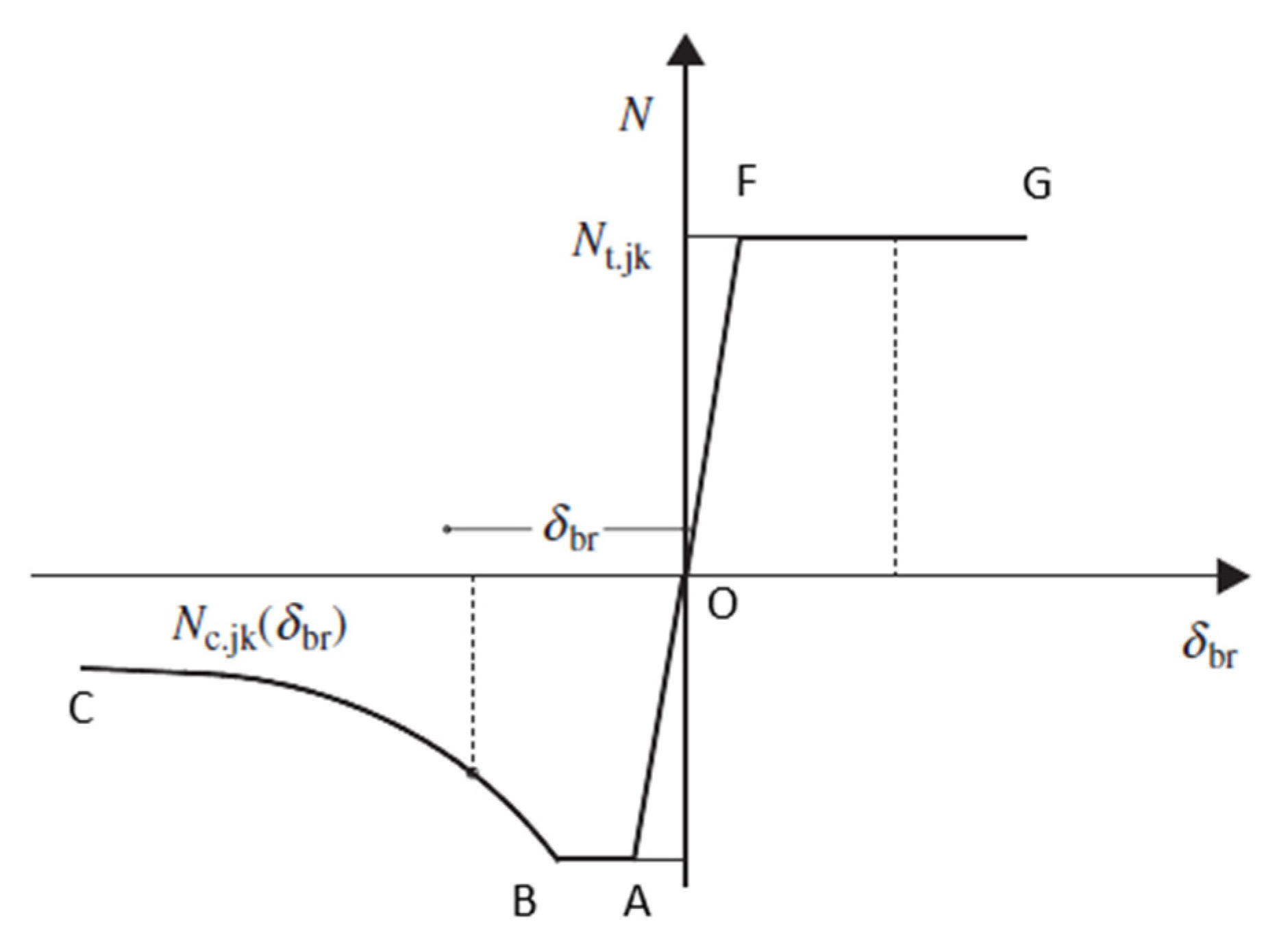
The axial force $N_{c.jk}\left({\delta }_u\right)$ is defined through the first three branches of the Georgescu’s model [40,41]:

• OA branch:

$$P=\frac{EA}{L}{\delta }_{OA}=K_d{\delta }_{OA} with P limited to P_{crit}$$

(15)

• AB branch:

$$f_{tB}=\frac{M_{pl}}{P_{crit}}\left(1-\frac{P_{crit}}{P_y}\right)$$

(16)

$${\delta }_B=-\frac{P_{crit}L}{EA}+\frac{{\pi }^2}{4L}\left(f_{tB}{}^2-f_0{}^2\right)$$

(17)

• BC branch:

$$f_t=\frac{M_{pl}}{P}\left(1-\frac{P}{P_y}\right) with P generic<P_{crit}$$

(18)

$$f_0={\delta }_{BC}=-\frac{PL}{EA}+\frac{{\pi }^2}{4L}\left(f_t{}^2-f_0{}^2\right)$$

(19)

The link describing the monotonic behaviour of the diagonals is completed by defining the behaviour in tension, adding the branches OF and FG, as reported in Figure 2.

The slopes of the equilibrium curve for each type of mechanism can be defined as follows:

• For the global collapse mechanism:

$${\gamma }^{\left(g\right)}=\frac{1}{h_{n_s}}\frac{{{\displaystyle \sum }}_{k=1}^{n_s}{V}_k{h}_k}{{{\displaystyle \sum }}_{k=1}^{n_s}{F}_k{h}_k}$$

(20)

• For the type-1 mechanism:

$${\gamma }_{i_m}^{\left(1\right)}=\frac{1}{h_{i_m}}\frac{{{\displaystyle \sum }}_{k=1}^{i_m}{V}_k{h}_k+h_{i_m}{{\displaystyle \sum }}_{k=i_m+1}^{n_s}{V}_k}{{{\displaystyle \sum }}_{k=1}^{i_m}{F}_k{h}_k+h_{i_m}{{\displaystyle \sum }}_{k=i_m+1}^{n_s}{F}_k}$$

(21)

• For the type-2 mechanism:

$${\gamma }_{i_m}^{\left(2\right)}=\frac{1}{h_{n_s}-h_{i_m-1}}\frac{{{\displaystyle \sum }}_{k=i_m}^{n_s}{V}_k\left(h_k-h_{i_m-1}\right)}{{{\displaystyle \sum }}_{k=i_m}^{n_s}{F}_k(h_k-h_{i_m-1})}$$

(22)

• For the type-3 mechanism:

$${\gamma }_{i_m}^{\left(3\right)}=\frac{1}{h_{i_m}-h_{i_m-1}}\frac{{{\displaystyle \sum }}_{k=i_m}^{n_s}{V}_k}{{{\displaystyle \sum }}_{k=i_m}^{n_s}{F}_k}$$

(23)

• Maximum multiplier according to calibrated Merchant–Rankine formula [52,53]:

$${\alpha }_{max}=\frac{{\alpha }_0}{1+{\Psi }_{CBF}{\alpha }_0{\gamma }_s{\delta }_1}$$

(24)

where

$${\Psi }_{CBF}=a+b{\xi }_{CBF}$$

(25)

$${\xi }_{CBF}=\frac{{{\displaystyle \sum }}_{n_{b_c}}\frac{E{A}_{diag}}{L_{diag}}·\frac{1}{1+{(L_b/h)}^2}}{{{\displaystyle \sum }}_{n_c}\frac{E{I}_c}{h^3}}$$

(26)

The use of Equation (4) is proposed by assuming, for the coefficient Ψ, the following relation considering GCBFs and SCBFs:

$${\Psi }_{CBF}=1.00421+0.10265 {\xi }_{CBF}$$

(27)

The coefficient Ψ_CBF has been derived also considering separately GCBFs and SCBFs. For global concentrically braced frames,

$${\Psi }_{CBF}=1.410677+0.294433 {\xi }_{CBF}$$

(28)

whereas, for special concentrically braced frames,

$${\Psi }_{CBF}=0.18799+0.11338 {\xi }_{CBF}$$

(29)

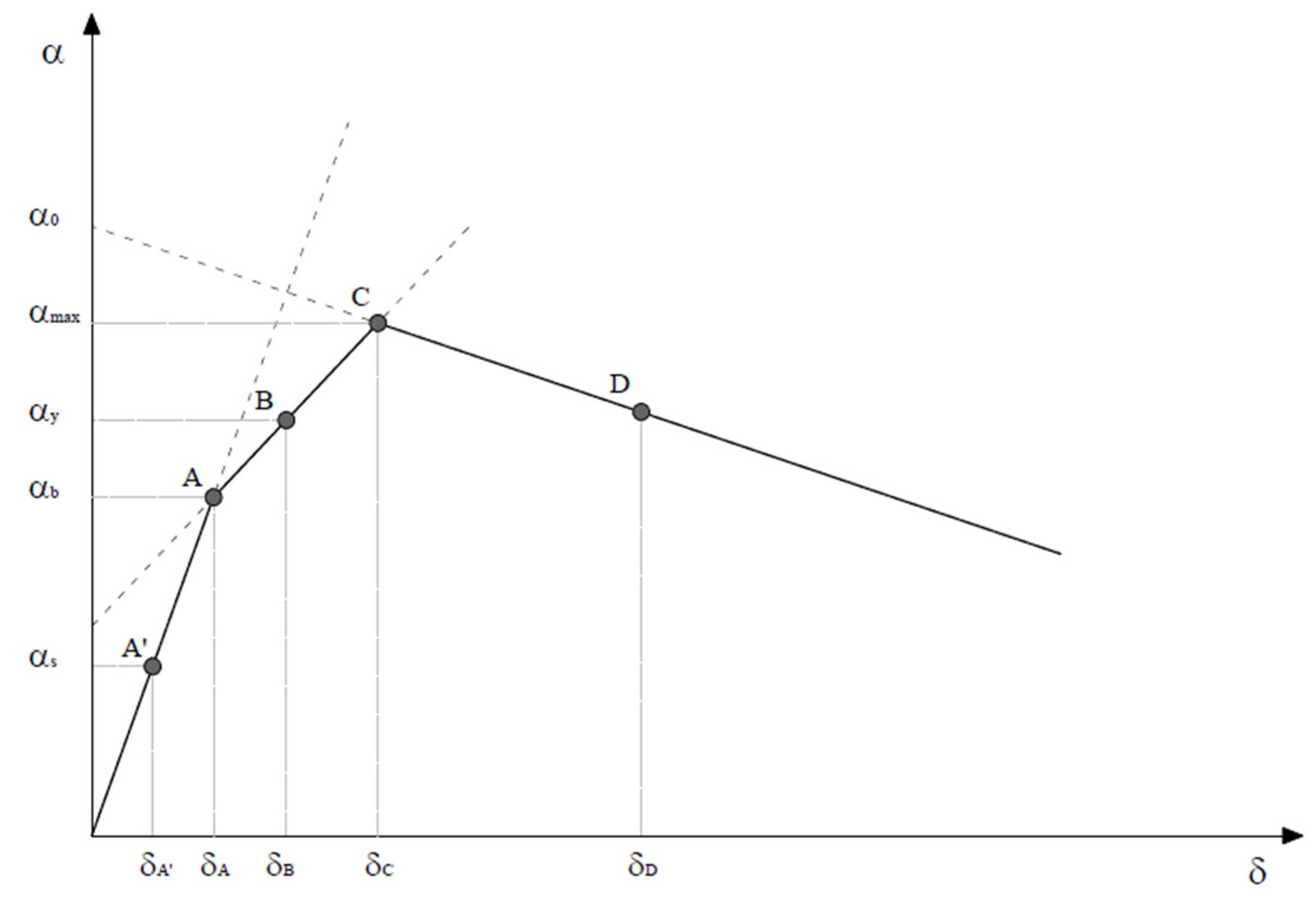
The characteristic performance points of the capacity curve (points A, B, C, D of Figure 3) have been identified on the trilinear model. The points are associated with specific limit states [50], provided by codes, identifying the achievement of a specific performance level [47,54,55,56].

• Point A—“Fully Operational”

$${\alpha }_{b,s}={\alpha }_A=\frac{1}{{\delta }_1}{\delta }_A$$

(30)

• Point B—“Operational”

$${\alpha }_B={\alpha }_A+K\text{'}\left({\delta }_B-{\delta }_A\right) ; {\delta }_B=\frac{{\alpha }_y-{\alpha }_A}{K\text{'}}+{\delta }_A$$

(31)

• Point C—“Life Safety”

$${\alpha }_C={\alpha }_0-{\gamma }_s\left({\delta }_C-{\delta }_y\right) ; {\delta }_C=\frac{{\alpha }_0-{\alpha }_A+K\text{'}{\delta }_A}{K^{\prime }+{\gamma }_s}$$

(32)

This point is determined through the intersection of the second elastic branch with the softening branch, representative of the collapse mechanism equilibrium curve.

• Point D—“Near Collapse”

$${\delta }_D={\delta }_C+{\phi }_{lim}·H_0$$

(33)

$${\delta }_D={\delta }_C+\left(\frac{{\delta }_{d,cp}}{h_i·\cos \theta }\right)·H_0$$

(34)

The inelastic deformation capacity for compressed braces (

Table 1. Capacity in terms of axial deformation for braces in compression.

	Limit State
Class of Cross-Section	DL	SD	NC
1	0.25 ΔC	4.0 ΔC	6.0 ΔC
2	0.25 ΔC	1.0 ΔC	2.0 ΔC

) is expressed in terms of the axial deformation of the brace, as a multiple of the axial deformation of the brace corresponding to buckling load Δ_c.

For braces in tension (

Table 2. Capacity in terms of axial deformation for braces in compression.

Limit State
DL	SD	NC
0.25 ΔC	7.0 ΔC	9.0 ΔC

), the inelastic deformation capacity should be expressed in terms of the axial deformation of the brace as a multiple of the axial deformation of the brace at tensile yielding load Δt.

3. Assessment Procedure in Terms of Spectral Accelerations According to ADRS Spectrum

The capacity–demand assessment procedure can be expressed through the ADRS spectrum. For each limit state, the spectrum $S_a-S_{De}$will be be defined by means of the relationship $S_{De}\left(T\right)=S_a\left(T\right){\left(T/2\mathsf{\pi }\right)}^2$. With regard to the capacity, it is necessary to represent the performance points of the behavioral curve of the structure in the ADRS plane. Of these points, it will be necessary to obtain the displacements $d_{LS}^{\ast }=d_{LS}/\Gamma$.

The cases $T^{\ast }>T_C$ and $T^{\ast }<T_C$. If $T^{\ast }>T_C$ must be distinguished [48]. The capacity in terms of spectral acceleration, relative to the limit state considered, can be obtained as follows:

$$S_{aSL}=d_{LS}^{\ast }{\omega }_0^{\ast }{}^2$$

(35)

The demand is represented by the spectral acceleration provided by the code, for the specific limit state, in the case of the equivalent SDOF system with the equivalent period of vibration T*.

For the assessment procedure, the inequality $S_{als}\ge S_a\left(T^{\ast }\right)$must be satisfied.

If $T^{\ast }<T_C$ and q > 1, according to the equality of energy criteria, there is a different procedure to evaluate the capacity that leads to the anelastic spectrum:

$$F_{ls}^{\ast }=\frac{m^{\ast }{S}_a\left(T^{\ast }\right)}{q_{ls}}$$

(36)

$$q_{ls}=1+\left({\mu }_{ls}-1\right)\frac{T^{\ast }}{T_C}$$

(37)

$$S_{aSL}=q_{ls}\frac{F_{ls}^{\ast }}{m^{\ast }}$$

(38)

If $T^{\ast }<T_C$ and q $\le$ 1, it results in:

$$F_{SL}^{\ast }=m^{\ast }{S}_a\left(T^{\ast }\right)$$

(39)

$$S_{aSL}=\frac{F_{ls}^{\ast }}{m^{\ast }}$$

(40)

$$m^{\ast }={\displaystyle \sum }_{k=1}^n{m}_k{·}_k$$

(41)

The checking is verified when the inequality $S_{als}\ge S_a\left(T^{\ast }\right)$is satisfied.

4. Assessment Procedure in Terms of Spectral Accelerations According to Nassar and Krawinkler

In the framework of capacity–demand checking [52,53,54,55,56,57,58], an equivalent SDOF system replaces the MDOF actual system exploiting the modal participation factor Γ. The capacity curve is reported in a ${\mathrm{F}}_{\mathrm{b}}$-${\mathrm{d}}_{\mathrm{c}}$ plane by multiplying α with the design base shear force. Then the capacity curve must be reduced through the modal participation factor and represented in a F*-d* plane. The demand is estimated according to the equivalent period T* and the equivalent mass m* as reported by the European codes. The capacity in terms of spectral acceleration for the points A, B, C, D is defined as follows:

• Point A—“Fully Operational”

$$S_{aFO}\left(T^{\ast }\right)=\frac{F_{FO}^{\ast }}{m^{\ast }}$$

(42)

• Point B—“Operational”

$$S_{aO}\left(T^{\ast }\right)=\frac{F_O^{\ast }}{m^{\ast }}$$

(43)

• Point C—“Life Safety”

$$F_{LS}^{\ast }=m^{\ast }{S}_{aLS}\left(T^{\ast }\right)$$

(44)

$$S_{aLS}\left(T^{\ast }\right)=\frac{F_{LS}^{\ast }}{m^{\ast }}$$

(45)

• Point D—“Near Collapse”

$$S_{aNC}\left(T^{\ast }\right)=\frac{F_{NC}^{\ast }}{m^{\ast }}{q}_{NC}$$

(46)

$$q_{NC}=\frac{q_0}{\phi }$$

(47)

$$q_0\left(\mu ,T,{\gamma }_{=0}\right)={\left[c\left({\mu }_{NC}-1\right)+1\right]}^{\raisebox{1ex}{$1$}\!\left/ \!\raisebox{-1ex}{$c$}\right.}$$

(48)

where $c=\frac{T^{\ast }}{1+T^{\ast }}+\frac{0.42}{T^{\ast }}$ and ${\mu }_{NC}=\frac{d_{NC}{}^{\ast }}{d_O{}^{\ast }}$

$$\phi =\frac{1+0.62{\left({\mu }_{NC}-1\right)}^{1.45}\gamma }{\left(1-\gamma \right)}$$

(49)

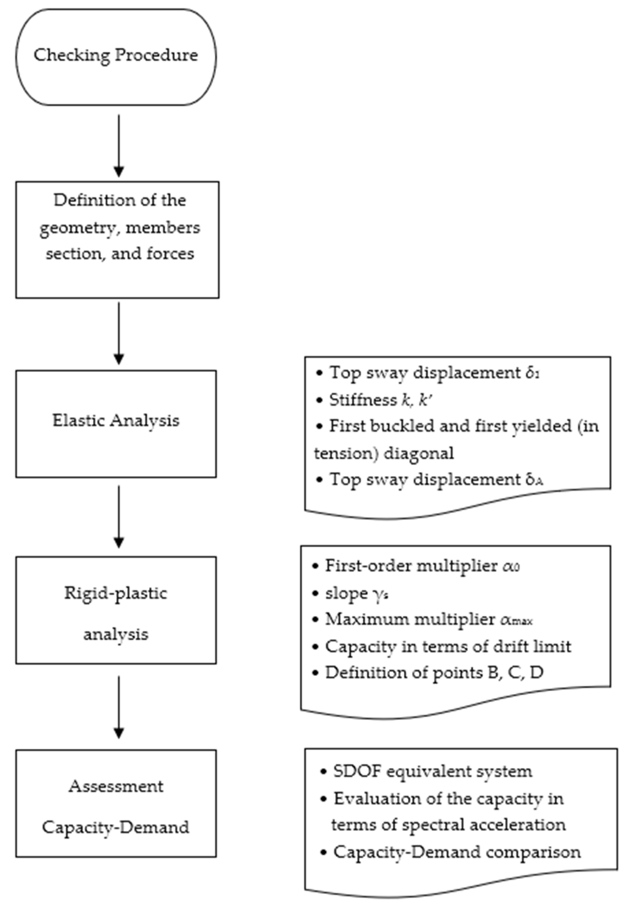
5. Numeric Examples

The simplified assessment procedure is applied to evaluate the capacity of three steel Concentrically Braced Frames designed according to three different approaches. Permanent loads ${\mathrm{G}}_{\mathrm{k}}$ are equal to 3.5 kN/m² wile live loads ${\mathrm{Q}}_{\mathrm{k}}$ equal to 3 kN/m². A frame tributary length of 6.00 m has been considered for the evaluation of gravitational loads acting on the beams. The steel used is S275.

A flowchart of the procedure is reported in Figure 4.

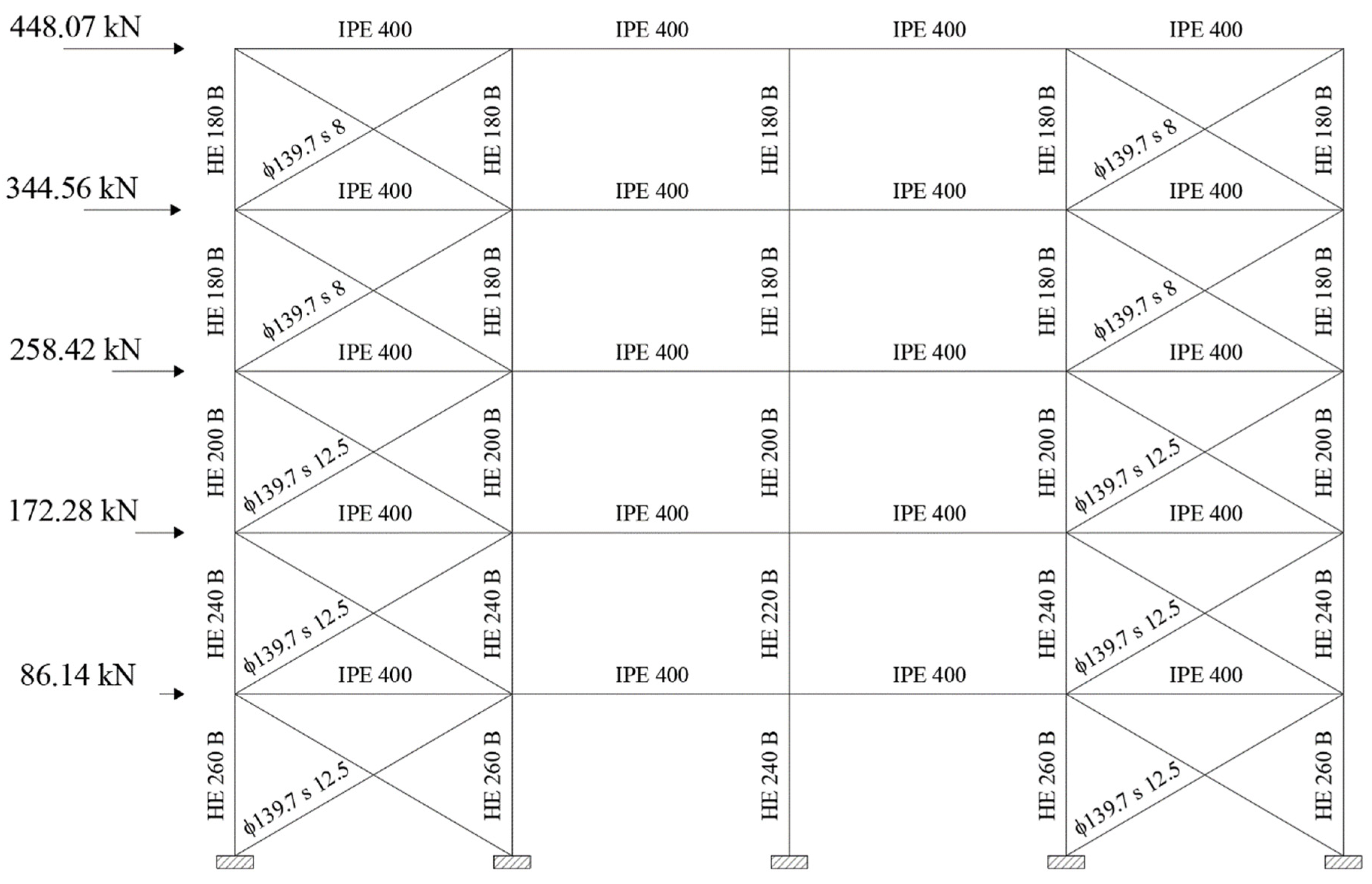
5.1. Global Concentrically Braced Frame

Global concentrically braced frames are designed according to the TPMC. The beams, diagonals, and column sections are reported in Figure 5.

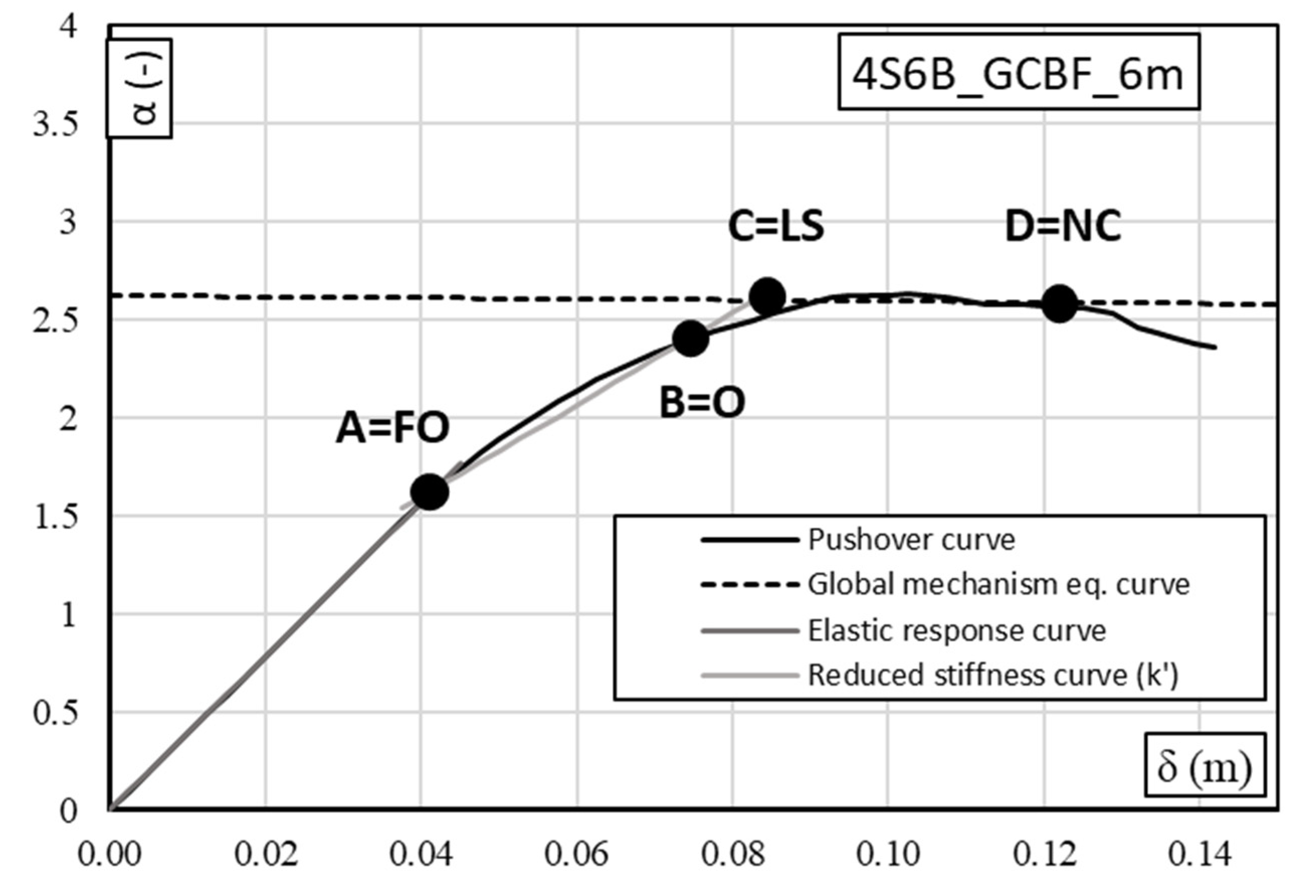
The trilinear capacity curve, showing the characteristic points of the model, is re-ported in Figure 6.

Parameters obtained from the elastic analysis:

• ${\delta }_1\left(\alpha =1\right)=$ 0.0255 m;
• $K=$ 39.161 m⁻¹;
• $K^{\prime }=$23.4964 m⁻¹;
• ${\delta }_A\left(1^{st} \mathrm{buckling}\right)=$0.0426 m;
• ${\alpha }_A=k{\delta }_A=$1.6577.

Parameters obtained from the rigid plastic analysis:

• ${\alpha }_0=$2.598;
• ${\gamma }_s=$0.285 m⁻¹;
• $\alpha ={\alpha }_0-{\gamma }_s\left(\delta -{\delta }_y\right) \to \alpha =2.598-0.285(\delta -$0.07438$)$;
• $\alpha \left(\delta =0\right)={\alpha }_0+{\gamma }_s{\delta }_y=$ 2.620;
• $H_0=14 m$ (global collapse mechanism).

Evaluation of the maximum multiplier through the calibrated Merchant–Rankine formula:

• ${\alpha }_{max}=\frac{{\alpha }_0}{1+{\Psi }_{CBF}{\alpha }_0{\gamma }_s{\delta }_1}=$2.5058

where

• ${\mathsf{\Psi }}_{\mathrm{CBF}}=\mathrm{a}+{\mathrm{b}\mathsf{\xi }}_{\mathrm{CBF}}=1.41068+0.29443{ \mathsf{\xi }}_{CBF}=1.698909$;
• with ${\mathsf{\xi }}_{\mathrm{CBF}}=\frac{{{\displaystyle \sum }}_{{\mathrm{n}}_{{\mathrm{b}}_{\mathrm{c}}}}\frac{{\mathrm{EA}}_{\mathrm{diag}}}{{\mathrm{L}}_{\mathrm{diag}}}·\frac{1}{1+{({\mathrm{L}}_{\mathrm{b}}/\mathrm{h})}^2}}{{{\displaystyle \sum }}_{{\mathrm{n}}_{\mathrm{c}}}\frac{{\mathrm{EI}}_{\mathrm{c}}}{{\mathrm{h}}^3}}$ = 1.945191;
• consequently ${\mathsf{\delta }}_{\mathrm{B}}=\frac{{\mathsf{\alpha }}_{\mathrm{y}}-{\mathsf{\alpha }}_{\mathrm{A}}}{\mathrm{K}\prime }+{\mathsf{\delta }}_{\mathrm{A}}=$0.07438;
• and ${\delta }_C=\frac{{\alpha }_0-{\alpha }_A+K\text{'}{\delta }_A}{K^{\prime }+{\gamma }_s}=$ 0.08163.

According to the limitations given by Eurocode 8 for compressed diagonals at Near Collapse limit state (Δ_c$·$6), the ultimate displacement is evaluated as:

• ${\delta }_D=\left(\frac{{\delta }_{d,cp}}{h_i·\cos \theta }\right)·H_0$ = $\left(\frac{0.026874}{3.5\times 0.86378}\right)\times 14=0.12445 m$

The checking procedures exploit the transformation of the MDOF system into an equivalent SDOF system through the participation factor of the main vibration mode Γ. For this reason, it is necessary to define:

• The eigenvector $\underset{\_}{ɸ}=\left\{{ɸ}_1,{ɸ}_2,{ɸ}_3,{ɸ}_4\right\}$ that, assuming ${ɸ}_k=\frac{F_k}{F_n}$, is:
  ${ɸ}_1=0.2398 {ɸ}_2=0.4795 {ɸ}_3=0.7193$
  ${ɸ}_4=1.00$

• The modal participation factor Γ:

$$\Gamma =\frac{{{\displaystyle \sum }}_{k=1}^n{m}_k{\Phi }_k}{{{\displaystyle \sum }}_{k=1}^n{m}_k{\Phi }_k{}^2}=1.343$$

being

$$\begin{gathered} m_1=278.75\times {10}^3 \mathrm{kg} m_2=278.75\times {10}^3 \mathrm{kg} m_3=278.75\times {10}^3\mathrm{kg} \\ {m}_4=290.64\times {10}^3 \mathrm{k} \end{gathered}$$

• The dynamic parameters of the equivalent SDOF system (Table 3).

Table 3. Dynamic parameters of the equivalent SDOF system (GCBF).

m*	k*	ω*	T*
[kg 103]	[kN/m]	[rad/s]	[s]
691.67	92,569.9	11.5688	0.5431

Table 3. Dynamic parameters of the equivalent SDOF system (GCBF).

m*	k*	ω*	T*
[kg 103]	[kN/m]	[rad/s]	[s]
691.67	92,569.9	11.5688	0.5431

Consequently, the performance points of the capacity curve are defined in the planes $\alpha -\delta$, $F_b-d_c$, $F^{\ast }-D^{\ast }$, $S_a-S_D$ assessing the capacity in terms of accelerations for both Nassar & Krawinkler and ADRS spectrum approaches. In

Table 4. ADRS spectrum approach (GCBF).

	FO	O	LS	NC
F [kN]	3918.52	5683.83	6086.44	6057.55
F* [kN]	2917.66	4232.08	4531.86	4510.35
d [m]	0.0426	0.0751	0.08163	0.12445
d* [m]	0.0317	0.0559	0.0608	0.0927
Sa* [g]	0.433	0.763	0.829	0.9803

and

Table 5. Nassar and Krawinkler approach (GCBF).

	FO	O	LS	NC0
F [kN]	3918.52	5683.83	6086.44	6141.53
F* [kN]	2917.66	4232.08	4531.86	4572.88
d [m]	0.0426	0.0751	0.08163	0.12445
d* [m]	0.0317	0.0559	0.0608	0.0927
μ [m]	-	-	-	1.524
Sa* [g]	0.430	0.624	0.6679	1.0177

the results, based on the ADRS spectrum the Nassar & Krawinkler formulation, are respectively reported.

Seismic performance verification requires that, for each limit state, the inequality ${\mathrm{S}}_{\mathrm{a}.\mathrm{SL}}{\left({\mathrm{T}}^{\ast }\right)}_{\mathrm{capacity}}\ge {\mathrm{S}}_{\mathrm{a}.\mathrm{SL}}{\left({\mathrm{T}}^{\ast }\right)}_{\mathrm{demand}}$ is satisfied.

5.2. Special Concentrically Braced Frame

Special concentrically braced frames are designed to fulfil the Eurocode 8 seismic provisions. The selected case study with the definition of the beam, diagonals, and column sections is reported in Figure 7.

The trilinear capacity curve, showing the characteristic points of the model, is re-ported in Figure 8.

Parameters obtained from the elastic analysis:

• ${\delta }_1\left(\alpha =1\right)=$ 0.06133 m;
• $K=$ 16.305 m⁻¹;
• $K^{\prime }=$13.044 m⁻¹;
• ${\delta }_A\left(1^{st} \mathrm{buckling}\right)=$0.0571 m;
• ${\alpha }_A=k{\delta }_A=$0.9311.

Parameters obtained from the rigid plastic analysis:

• ${\alpha }_0=$1.763;
• ${\gamma }_s=$0.185 m⁻¹;
• $\alpha ={\alpha }_0-{\gamma }_s\left(\delta -{\delta }_y\right) \to \alpha =1.763-0.185\left(\delta -0.1171\right)$;
• $\alpha \left(\delta =0\right)={\alpha }_0+{\gamma }_s{\delta }_y=$ 1.785;
• $H_0=21 m$ (global collapse mechanism).

Evaluation of the maximum multiplier through the calibrated Merchant–Rankine formula:

• ${\alpha }_{max}=\frac{{\alpha }_0}{1+{\Psi }_{CBF}{\alpha }_0{\gamma }_s{\delta }_1}=$1.7267

where

• ${\mathsf{\Psi }}_{\mathrm{CBF}}=\mathrm{a}+{\mathrm{b}\mathsf{\xi }}_{\mathrm{CBF}}=1.00421+0.10265{ \mathsf{\xi }}_{CBF}=1.05338$;
• With ${\mathsf{\xi }}_{\mathrm{CBF}}=\frac{{{\displaystyle \sum }}_{{\mathrm{n}}_{{\mathrm{b}}_{\mathrm{c}}}}\frac{{\mathrm{EA}}_{\mathrm{diag}}}{{\mathrm{L}}_{\mathrm{diag}}}·\frac{1}{1+{({\mathrm{L}}_{\mathrm{b}}/\mathrm{h})}^2}}{{{\displaystyle \sum }}_{{\mathrm{n}}_{\mathrm{c}}}\frac{{\mathrm{EI}}_{\mathrm{c}}}{{\mathrm{h}}^3}}$ = 0.47899;
• consequently ${\mathsf{\delta }}_{\mathrm{B}}=\frac{{\mathsf{\alpha }}_{\mathrm{y}}-{\mathsf{\alpha }}_{\mathrm{A}}}{\mathrm{K}\prime }+{\mathsf{\delta }}_{\mathrm{A}}=$0.1171;
• and ${\delta }_C=\frac{{\alpha }_0-{\alpha }_A+K\text{'}{\delta }_A}{K^{\prime }+{\gamma }_s}=$ 0.11922.

According to the limitations given by Eurocode 8 for compressed diagonals at Near Collapse limit state (Δ_c$·$6), the ultimate displacement is evaluated as:

• ${\delta }_D=\left(\frac{{\delta }_{d,cp}}{h_i·\cos \theta }\right)·H_0$ = $\left(\frac{0.026874}{3.5\times 0.86378}\right)\times 21=0.18667 m$

The checking procedures exploit the transformation of the MDOF system into an equivalent SDOF system through the participation factor of the main vibration mode Γ. For this reason, it is necessary to define:

• The eigenvector $\underset{\_}{ɸ}=\left\{{ɸ}_1,{ɸ}_2,{ɸ}_3,{ɸ}_4,{ɸ}_5,{ɸ}_6\right\}$ that, assuming ${ɸ}_k=\frac{F_k}{F_n}$, is:

$$\begin{gathered} {ɸ}_1=0.1598 {ɸ}_2=0.3197 {ɸ}_3=0.4795 \\ {ɸ}_4=0.6394 {ɸ}_5=0.7992 {ɸ}_6=1.00 \end{gathered}$$

• The modal participation factor Γ:

$$\Gamma =\frac{{{\displaystyle \sum }}_{k=1}^n{m}_k{ɸ}_k}{{{\displaystyle \sum }}_{k=1}^n{m}_k{ɸ}_k{}^2}=1.405$$

being

$$\begin{gathered} m_1=278.75\times {10}^3 \mathrm{kg} m_2=278.75\times {10}^3 \mathrm{kg} m_3=278.75\times {10}^3\mathrm{kg} \\ {m}_4=278.75\times {10}^3 \mathrm{kg} m_5=278.75\times {10}^3 \mathrm{kg} m_6=290.64\times {10}^3 \mathrm{kg} \end{gathered}$$

• The dynamic parameters of the equivalent SDOF system (Table 6).

Table 6. Dynamic parameters of the equivalent SDOF system (SCBF).

m*	k*	𝜔∗	T*
[kg 103]	[kN/m]	[rad/s]	[s]
959.01	57,610	7.75062	0.81067

Table 6. Dynamic parameters of the equivalent SDOF system (SCBF).

m*	k*	𝜔∗	T*
[kg 103]	[kN/m]	[rad/s]	[s]
959.01	57,610	7.75062	0.81067

Consequently, the performance points of the capacity curve are defined in the planes $\mathsf{\alpha }-\mathsf{\delta }$, ${\mathrm{F}}_{\mathrm{b}}-{\mathrm{d}}_{\mathrm{c}}$, ${\mathrm{F}}^{\ast }-{\mathrm{D}}^{\ast }$, ${\mathrm{S}}_{\mathrm{a}}-{\mathrm{S}}_{\mathrm{D}}$ assessing the capacity in terms of accelerations for both Nassar & Krawinkler and ADRS spectrum approaches. In

Table 7. ADRS spectrum approach (SCBF).

	FO	O	LS	NC
F [kN]	3290.01	6009.54	6151.51	6107.34
F* [kN]	2340.99	4276.06	4377.08	4345.65
d [m]	0.0571	0.1171	0.1192	0.1867
d* [m]	0.0406	0.0833	0.0848	0.1328
Sa* [g]	0.2488	0.4545	0.4653	0.8151

and

Table 8. Nassar and Krawinkler approach (SCBF).

	FO	O	LS	NC0
F [kN]	3290.01	6009.54	6151.51	6229.56
F* [kN]	2340.99	4276.06	4377.08	4432.62
d [m]	0.0571	0.1171	0.1192	0.1867
d* [m]	0.0406	0.0833	0.0848	0.1328
μ [m]	-	-	-	1.566
Sa* [g]	0.2488	0.4545	0.6525	0.7399

the results, based on the ADRS spectrum the Nassar & Krawinkler formulation, are respectively reported.

Seismic performance verification requires that, for each limit state, the inequality $S_{a.SL}{\left(T^{\ast }\right)}_{capacity}\ge S_{a.SL}{\left(T^{\ast }\right)}_{demand}$ is satisfied.

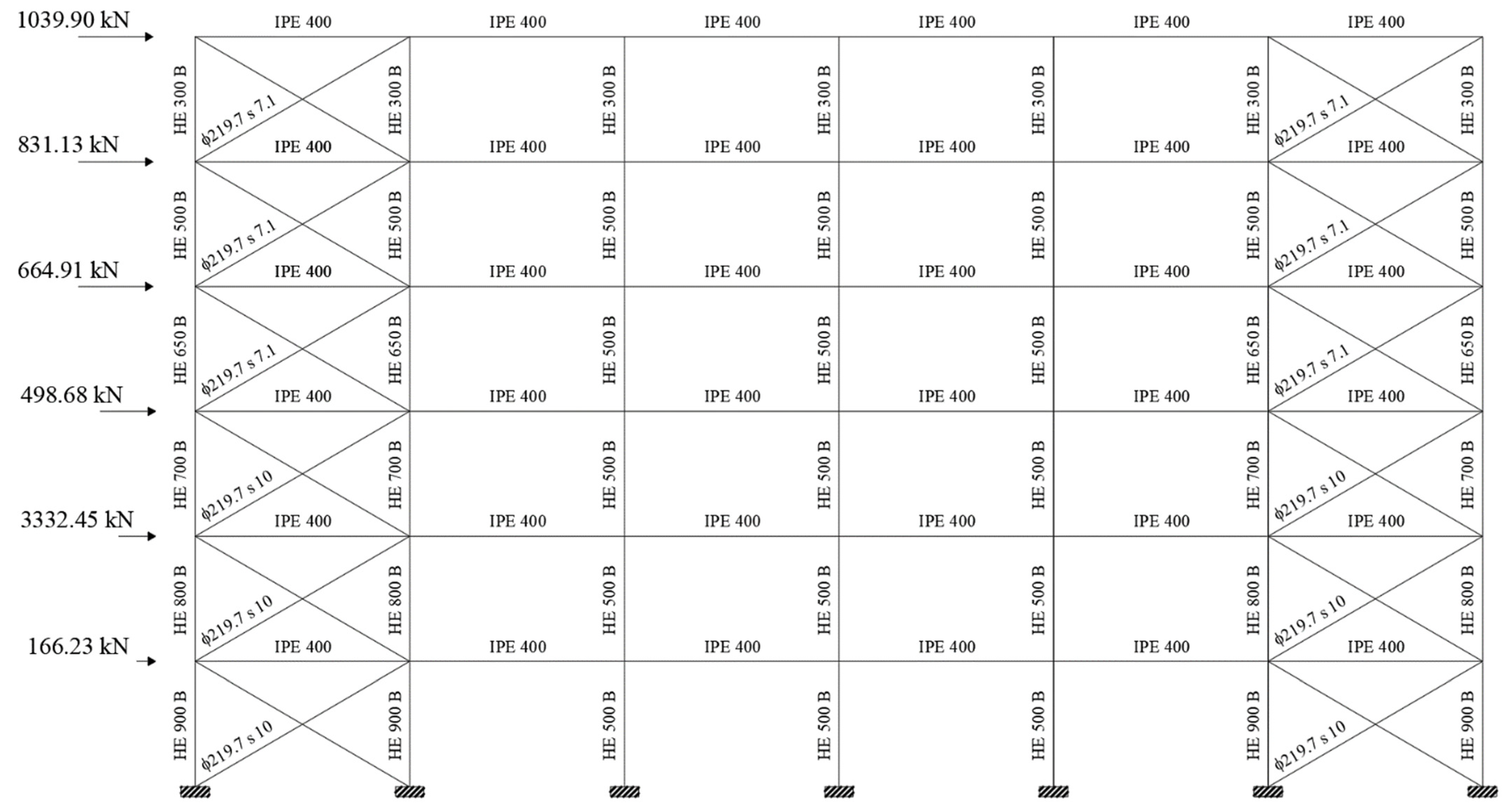
5.3. Ordinary Concentrically Braced Frame

Special concentrically braced frames are designed to fulfil the Eurocode 8 seismic provisions. The selected case study with the definition of the beam, diagonals, and column sections is reported in Figure 9.

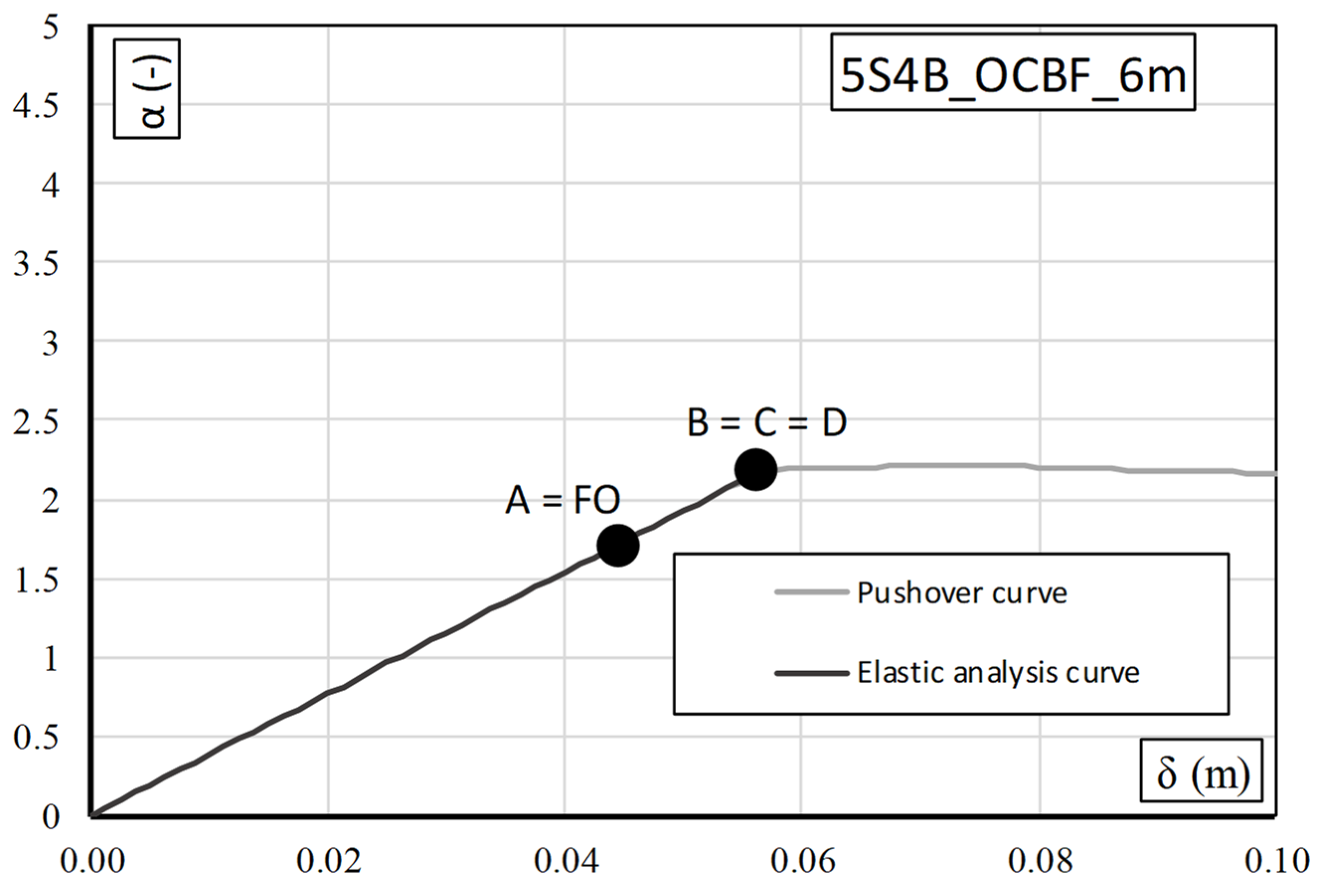
The trilinear capacity curve, showing the characteristic points of the model, is re-ported in Figure 10.

Parameters obtained from the elastic analysis:

• ${\delta }_1\left(\alpha =1\right)=$ 0.02597 m;
• $K=$38.501 m⁻¹;
• $K^{\prime }=$ 25.02;
• ${\delta }_A=$0.1602 m;
• ${\alpha }_A=k{\delta }_A=$2.0680.

It is not necessary to perform rigid plastic analysis because the buckling of columns occurs for a multiplier of horizontal forces very close to ${\alpha }_A$. Consequently,

• ${\delta }_u={\delta }_B={\delta }_C={\delta }_D=0.0575 m$;
• ${\alpha }_u={\alpha }_B={\alpha }_C={\alpha }_D=2.18596$.

The checking procedures exploit the transformation of the MDOF system into an equivalent SDOF system through the participation factor of the main vibration mode Γ. For this reason, it is necessary to define:

The eigenvector $\underset{\_}{ɸ}=\left\{{ɸ}_1,{ɸ}_2,{ɸ}_3,{ɸ}_4,{ɸ}_5\right\}$ that, assuming ${ɸ}_k=\frac{F_k}{F_n}$, is:

$$\begin{gathered} {ɸ}_1=0.192 {ɸ}_2=0.384 {ɸ}_3=0.575 \\ {ɸ}_4=0.767 {ɸ}_5=1.00 \end{gathered}$$

The modal participation factor Γ:

$$\Gamma =\frac{{{\displaystyle \sum }}_{k=1}^n{m}_k{\Phi }_k}{{{\displaystyle \sum }}_{k=1}^n{m}_k{\Phi }_k{}^2}=1.379$$

being

$$\begin{gathered} m_1=123.89\times {10}^3 \mathrm{kg} m_2=123.89\times {10}^3 \mathrm{kg} m_3=123.89\times {10}^3\mathrm{kg} \\ {m}_4=123.89\times {10}^3 \mathrm{kg} m_5=129.17\times {10}^3 \mathrm{kg} \end{gathered}$$

and the dynamic parameters of the equivalent SDOF system (

Table 9. Dynamic parameters of the equivalent SDOF system (OCBF).

m*	k*	𝜔∗	T*
[kg 103]	[kN/m]	[rad/s]	[s]
366.82	37,127.6	10.061	0.6245

).

Therefore, the characteristic points of the capacity curve are defined in the planes $\mathsf{\alpha }-\mathsf{\delta }$, ${\mathrm{F}}_{\mathrm{b}}-{\mathrm{d}}_{\mathrm{c}}$, ${\mathrm{F}}^{\ast }-{\mathrm{D}}^{\ast }$, ${\mathrm{S}}_{\mathrm{a}}-{\mathrm{S}}_{\mathrm{D}}$ assessing the capacity in terms of accelerations for the Nassar and Krawinkler approach and ADRS spectrum approach. In particular, in

Table 10. ADRS spectrum approach (SCBF).

	FO	O	LS	NC
F [kN]	2235.76	2363.33	2363.33	2363.33
F* [kN]	1620.83	1713.31	1713.31	1713.31
d [m]	0.0538	0.0575	0.0575	0.0575
d* [m]	0.0390	0.0417	0.0417	0.0417
Sa* [g]	0.402	0.430	0.430	0.430

, results based on the use of the ADRS spectrum, and, in

Table 11. Nassar and Krawinkler approach (SCBF).

	FO	O	LS	NC0
F [kN]	2235.76	2363.33	2363.33	2363.33
F* [kN]	1620.83	1713.31	1713.31	1713.31
d [m]	0.0538	0.0575	0.0575	0.0575
d* [m]	0.0390	0.0417	0.0417	0.0417
μ [m]	-	-	-	-
Sa* [g]	0.450	0.476	0.476	0.476

, results based on the use of Nassar and Krawinkler formulation, are reported.

Seismic performance verification requires that, for each limit state, the inequality ${\mathrm{S}}_{\mathrm{a}.\mathrm{SL}}{\left({\mathrm{T}}^{\ast }\right)}_{\mathrm{capacity}}\ge {\mathrm{S}}_{\mathrm{a}.\mathrm{SL}}{\left({\mathrm{T}}^{\ast }\right)}_{\mathrm{demand}}$ is satisfied.

6. Conclusions

In this paper, three numeric examples explaining the application of a new simplified assessment procedure for CBFs are reported. The given numerical examples show the speed and ease of application of the method, which is completely analytical. The equations of the branches constituting the trilinear model can be obtained uniquely, given the horizontal seismic actions and the sections of diagonals and columns of the analyzed frame. For this reason, this methodology is strongly suggested for the large-scale assessment of the seismic vulnerability of the built heritage. In addition, it constitutes a suitable tool for checking the capacity of the buildings designed with the new seismic code prescriptions, or for an evaluation of seismic vulnerability in the immediate aftermath of an earthquake. The reliability of the procedure is testified by an extensive regression analysis, carried out on 420 CBFs designed according to different approaches, belonging to different historical periods. In the sample cases, it is evident that the descending branch has an average slope like the one resulting from the pushover, while the difference in terms of the multiplier is due to the elastic deformability, which is not included in a rigid plastic model.

The feasibility of the procedure is very high and makes it suitable to be applied indiscriminately to frames belonging to different historical periods.

The scatter between the values computed from the pushover analysis and the proposed method of the maximum bearing multiplier α and the displacement corresponding to the collapse and formation of the plastic mechanism is usually lower than 10%, testifying the accuracy of the proposed formulations. In addition, the results achieved by the simplified assessment procedure are mainly on the safe side.

The assessment of structure vulnerability, in terms of a comparison of the capacity–demand, has also been performed by using the Nassar and Krawinkler approach, which is characterized by a wide generality because it does not discriminate between high and low periods of vibration and accounts for second-order effects.

It is important to mention that the code assessment approach does not provide the definition of specific performance points on the pushover curve. The user must identify target limits, which are provided by codes in terms of displacements. In the proposed methodology, on the other hand, specific limit states are also associated with performance points, making the capacity–demand comparison process immediate. The discretization of the trilinear model in characteristic points (A, B, C, D), associated with the achievement of predefined performance objectives, makes the comparison between the capacity and demand for each limit state given by codes easy.