1. Introduction
Short fiber-reinforced plastics are ideal materials for high-performance lightweight applications. This usually requires a very accurate numerical determination of the mechanical stresses by structural simulations during the engineering process of technical products. This can be a major challenge: If short glass fiber reinforced thermoplastics are processed by injection molding or other primary forming processes, there is a direct correlation between the resulting mechanical properties of the material and the manufacturing process. This is caused by locally different microstructures, since the spatial orientation of the short fibers of the composite material varies at each point of the molded part depending on the flow conditions over time during the manufacturing process. Therefore, it is obvious to describe the mechanical behavior of the component as a function of the fiber orientation. Consequently, the more precisely the fiber orientation can be modelled, the more precisely the mechanical design of the molded part can be performed.
In injection molding simulation, the mathematical description of the fiber orientation is significantly simplified due to the very high numerical effort required otherwise. Reconstruction methods are used to recover the original fiber orientation in a post-processing step from the orientation tensor. In this paper, the performance of two reconstruction methods was compared and analyzed. The reconstruction methods involved the spherical harmonics and the maximum entropy method. The analysis was performed as follows: Test scenarios were developed, and the fiber orientation was calculated using both reconstruction methods. A subsequent comparison between reconstructed and original fiber orientation shows the quality of the reconstruction as well as its calculation effort. The developed test scenarios allowed the comparison of the two reconstruction methods for a much larger spectrum of different fiber orientation compared to experimental tests of injection molded specimens. Furthermore, it is possible to evaluate the reconstruction methods independently from any process simulation.
The aim of this paper was to show the advantages and disadvantages of the individual reconstruction methods.
2. Fiber Orientation
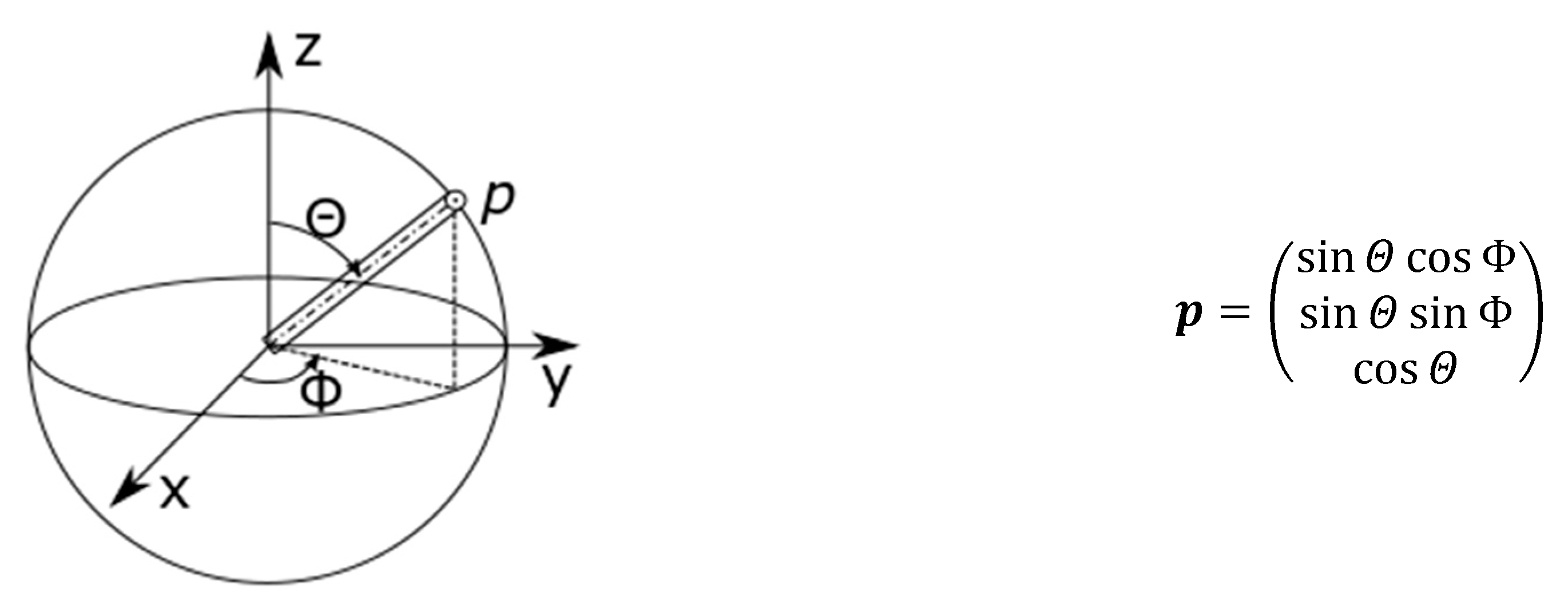
The orientation of a single fiber in space can be given as a direction vector
in spherical coordinates on the unit sphere
(see
Figure 1). Here, the angle
is defined as between
and
, and
between
and
.
The change of the orientation
of a fiber in a fluid–fiber suspension of velocity
can be modeled basically with Jeffrey’s equation [
1]. Jeffrey describes the movement of ellipsoidal particles in a viscous fluid under the condition of a laminar flow. For a Newtonian fluid without externally applied moments, the change of the orientation
is:
The vorticity tensor ω is calculated by:
and the strain rate tensor
with:
The constant:
is the fiber geometry factor, which is determined by the fiber aspect ratio
of fiber length
and fiber diameter
. In a simple shear flow, the solution of the Jeffrey equation is periodic in time. This means that after some time, a single fiber rotates back to its initial position. Jeffrey’s equation is a useful model for the calculation of fiber orientation in the case of a thin suspension [
2]. Thin means in this case that the fibers can statistically rotate undisturbed in the suspension. For suspensions with higher fiber concentrations as typically occur in technical relevant short-fiber reinforced plastics, fiber interaction plays an important role. Hence, Jeffery’s equation alone is not applicable here. The suspensions can be classified according to the fiber volume content
and the aspect ratio
[
2]. The classification is listed in
Table 1.
In technical applications, typically, there are between 2000 and 20,000 fibers per cubic millimeter, depending on the fiber volume content. Therefore, a deterministic consideration of the fiber orientation of each individual fiber is not feasible due to this large number, and a statistical analysis is carried out accordingly. The fiber orientation density function (ODF)
is defined for all fibers in the unit sphere. It indicates the probability of a fiber pointing in a certain direction
. The ODF is periodic, i.e.,
applies. Furthermore, a normalization condition is given by:
The statistical consideration of the fiber orientation allows the use of the so-called Fokker–Plank equation for the calculation. The Fokker–Planck equation generally describes the change of a distribution function of fluctuating macroscopic variables [
3]. The first application of the Fokker–Planck equation was to calculate the Brownian motion [
4]. In its simplest, one-dimensional form, the Fokker–Plank equation is given by:
is a distribution function, depending on a variable
. The variable
is called the drift part and
the diffusion part. Both the drift and diffusion part can be determined on the basis of the microscopic behavior or derived from the statistical behavior on the macroscopic level. In the context of fiber orientation, the drift part corresponds to the part induced by hydrodynamic forces, and the diffusion part corresponds to the fiber interaction. To calculate the ODF, Jeffrey’s equation can be used for the drift part of the Fokker–Plank equation. For the diffusion part, an approach for fiber interaction with:
is used. The Fokker–Planck equation for an ODF
therefore results in:
Solving the Fokker–Plank equation within the framework of an injection molding simulation is numerically very costly, since the differential equation has to be solved in 3D space on the unit sphere
. One possibility to reduce the computational effort is to decompose the ODF into moments of spherical harmonics. These moments are also known as fiber orientation tensors:
Folgar and Tucker apply the decomposition to the Fokker–Planck equation [
5]. For the second-order fiber orientation tensor, the resulting equation reads:
It should be noticed that the second-order orientation tensor depends on the fourth-order fiber orientation tensor
. Analogously, the fourth-order fiber orientation tensor can be calculated with:
Hereby, a dependency on the fiber orientation tensor of the next higher even-order
has to be considered. In order to solve the Folgar–Tucker equation, it is necessary to calculate the fiber orientation tensor of the next higher even order using an approximation. So-called closures offer the possibility for this purpose. Due to the fact that higher-order tensors contain, in principle, more information than lower-order tensors, a closure can only be based on assumptions. A list, including references, for further information of known closures for the fourth-order tensor is given in
Table 2 and for the sixth order in
Table 3.
The large number of closures developed and discussed in the literature shows that it is not evident to develop a comprehensive closure that is both numerically efficient and satisfactorily accurate. Commercial injection molding simulation programs usually use the hybrid or orthotropic closures for the fourth-order tensor [
23,
24], although it can be shown that more accurate closures exist [
10].
Not only is the accuracy of the closures discussed in the literature, but also the results of process simulations are a subject of many research projects. However, the second- and the fourth-order fiber orientation tensors are often used as the evaluation parameter and not the ODF—for example, in the work on the influence of fiber interaction [
10,
25], or for the processing of long fibers [
26]. Even in the work by Férec et al. [
27], in which the Fokker–Planck equation is solved, the fiber orientation tensors and not the ODF were used as evaluation criteria. Russel et al. investigated the prediction of the fiber orientation tensor in fused filament fabrication [
28], while Kuhn et al. in compression molding of long fibers.
However, the design process of components often requires the use of the ODF
and not only the fiber orientation tensors, i.e., structural simulations by the finite element method, generating a representative volume element (RVE) or calculating the effective stiffness
using a two-step homogenization [
29]:
Müller and Böhlke showed that the two-stage tensor is not sufficient to describe a microstructure in order to determine effective composite properties with sufficient accuracy [
30]. Therefore, it is absolutely necessary to investigate the quality of the reconstruction methods of an ODF on the basis of a fiber orientation tensor.
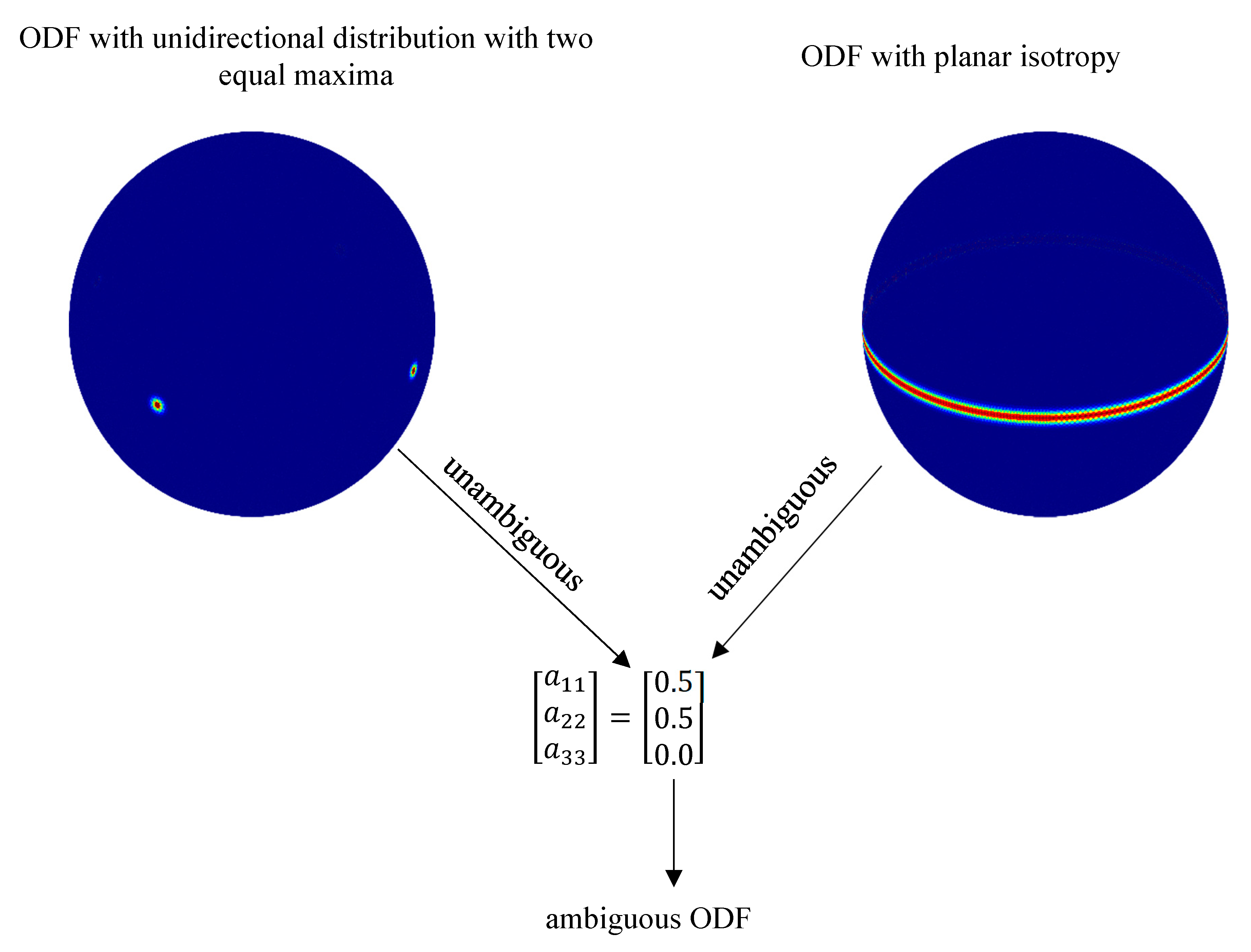
Due to the necessary knowledge of the ODF, a reconstruction problem arises, how an ODF can be derived from the fiber orientation tensor. This problem is ruled by the fact that the reconstruction of the ODF from the fiber orientation tensors is not unambiguous, as
Figure 2 illustrates. It shows two different ODFs: on the one hand, an ODF with planar isotropy, and on the other hand, one with unidirectional distribution of two equal maximas. The red color on the shown unit spheres indicates a high fiber probability density. The second-order fiber orientation tensors belonging to these two different ODFs are identical. This example explains that by knowing exclusively the fiber orientation tensor, there can be no unambiguous reconstruction of the ODF. Mathematically speaking, the reconstruction problem is ill-posed.
3. Icosphere
A discretization of the unit sphere is necessary in order to represent the ODF numerically. Equidistant angular steps of and in a polar coordinate system can be used in principle but are rather ineffective. Because of the inadequate spatial distribution of the resulting grid points on the surface of the unit sphere using equidistant angular steps, the density of the grid points at the poles is considerably higher than at the equatorial plane. Accordingly, depending on the choice of the angular steps, both the computational effort is too high and/or the resolution at the equatorial plane is too low.
Weber et al. used an improved formulation of the unit sphere using equidistant angular steps in the pole direction and azimuth angular steps as a function of the pole angle. This results in a surface grid with almost identical surface areas [
31]. However, the shapes of the surface areas are very different at the equatorial plane and the poles.
Another simple method to create a unit sphere with approximately the same density of grid points is to create an icosphere. The starting point of this method is a regular icosahedron, which is represented by the following 12 points:
| | | |
| | | |
| | | |
| | | |
with
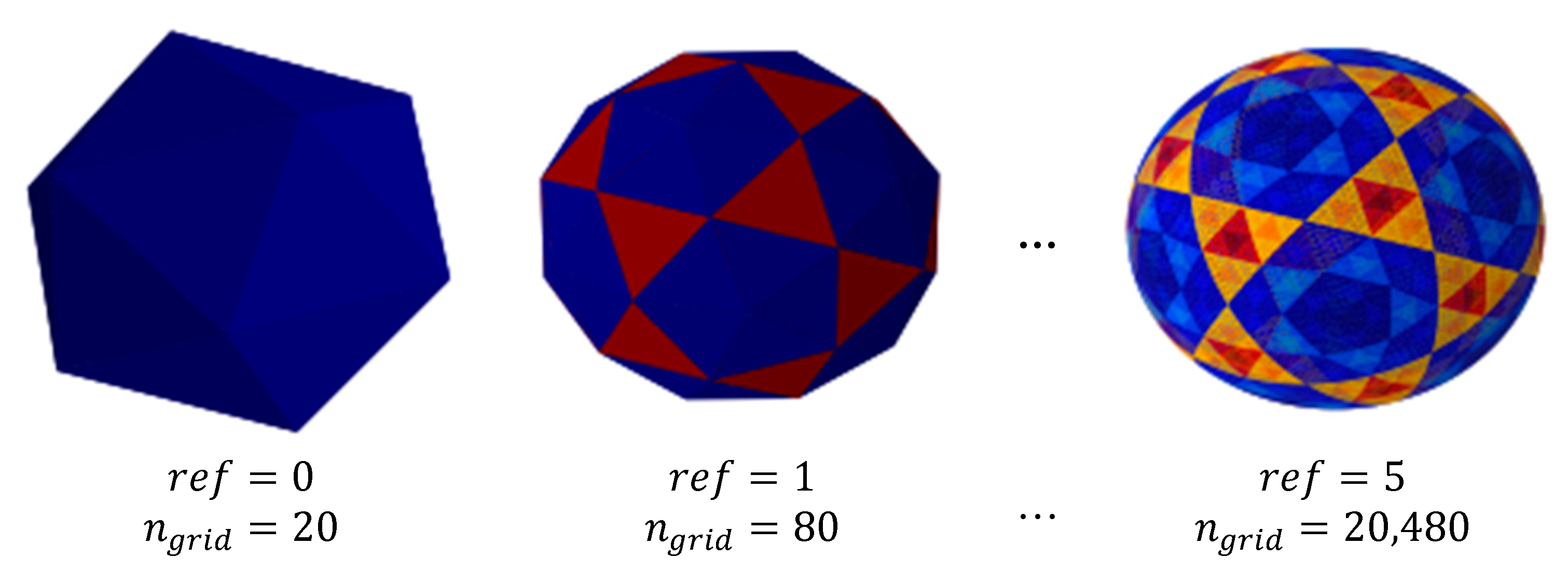
. The convex hull of the point cloud is the regular icosahedron. The convex hull consists of 20 triangles of equal size. To refine the regular icosahedron to the icosphere, each of the triangles is divided into 4 smaller triangles. For this purpose, the center of each edge of the triangles is calculated and projected onto the surface of the unit sphere. This procedure can be repeated as often as needed. In this paper, the center points of the surfaces were used as grid points for the evaluation of
. Therefore, the number of grid points
is equal to the number of triangles.
Figure 3 shows the evolution of the icosphere with increasing refinement level
. A refinement level of
with a total of 20,480 grid points was used entirely in this work.
5. Evaluation
The reconstruction methods were evaluated by comparing the results in terms of accuracy and computational effort. The basis for the investigation was provided by various test scenarios, whose creation is explained in more detail in the following section. One test scenario is an explicitly given initial ODF. This initial ODF was used to estimate the fiber orientation tensors, which were used as inputs for the reconstruction methods. With this approach, it is possible to compare the reconstructed ODFs against each other as well as against the initial ODF. Both the accuracy of the reconstruction and the numerical effort, measured by the required computing time, were compared. The spectral decomposition was repeated for the steps
to
. In addition, the higher-order tensors were calculated once from the initial ODF and once by closures from the lower-order tensors.
Table 4 gives an overview of the reconstruction methods used and their variants. The fiber orientation tensors used for the reconstruction are indicated. In the following, the methods are only indicated by their abbreviations. ME stands for maximum entropy and SH for spherical harmonics. The number after SH indicates the maximum order
used for the reconstruction. The abbreviation HY at the end stands for the use of the hybrid closure of the highest tensor, and HYHY for the consecutive use of the hybrid closure.
5.1. Tests Scenarios
Two different test variants of the test scenarios were considered. On the one hand, a fiber orientation was created on the basis of a Bingham distribution and, on the other hand, measured fiber orientation from the literature was used.
The idea of fiber orientation with a Bingham distribution is based on the solution of the Fokker–Plank equation. Chaubal and Leal limited the flow conditions at which a Bingham distribution of the Fokker–Planck equation can be expected [
13]. To create a Bingham distribution, the expected value μ and the covariance
are required. The expected value specifies the position of the maximum of the distribution. The covariance, on the other hand, determines the scattering width of the distribution. The expected value μ was exemplarily chosen to be on the equatorial plane with
. The covariance was varied in order to create the different test scenarios. The variation was chosen in such a way that the fiber orientation corresponds to unidirectional, orthotropic with respect to the equatorial and meridian plane, and quasi-isotropic conditions. For this purpose, α and β (see Equation (17)) were independently varied in 20 logarithmically equidistant steps from
to
resulting in a total of 400 individual test scenarios.
5.2. Evaluation Criteria
For the complete evaluation of the reconstruction methods, a measure of the similarity of two probability distributions
and
is required. For that, the sum of the squared errors between initial and computed ODF can be considered by:
A further measure for evaluation is the Kullback–Leibner distance [
42]:
which can be calculated by the Kullback–Leibner divergence:
A Kullback–Leibner distance of means that both probability distributions are identical. However, the greater the value of the Kullback–Leibner distance is, the more different the probability distributions are.
Some examples of comparisons between ODFs should illustrate the difference of the evaluation criteria.
Table 5 shows a total of 5 ODFs. Each of the 5 ODFs is compared with the first ODF
and the evaluation criteria are determined. This shows that the integral error
is by definition largest if the expected value is not identical (
and the distributions do not overlap. The Kullback–Leibner distance in this case is 0 because the distribution is the same. The Kullback–Leibner distance, on the other hand, is largest in the case of
. Thus, the Kullback–Leibner distance gives a more useful estimation with regard to the shape of the ODF.
5.3. Numerical Results for Bingham Distributions
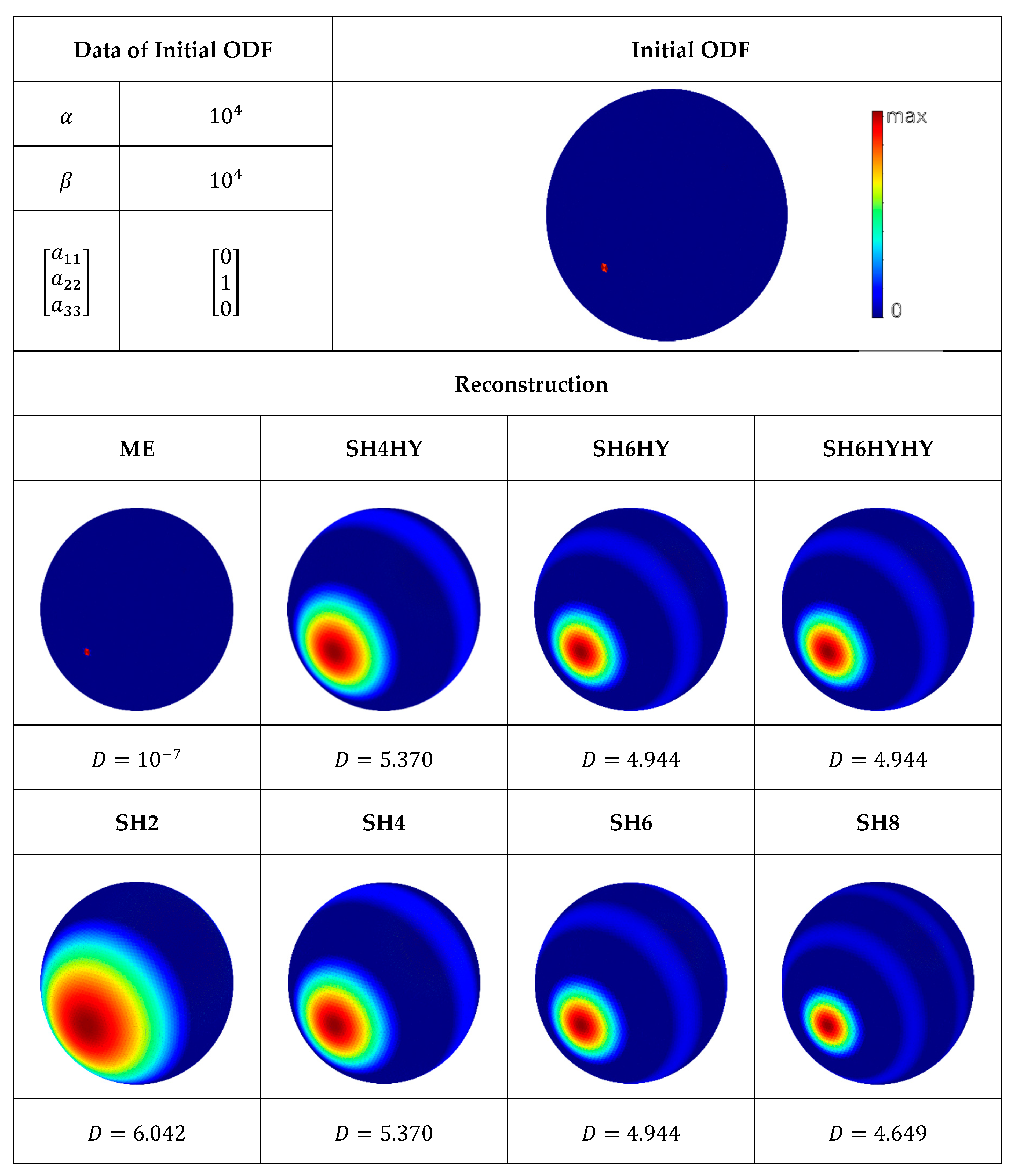
First, some selected test scenarios were evaluated in order to demonstrate the principal differences between the reconstruction methods. A total of five different test scenarios are presented as examples. Each of these five test scenarios represents a qualitatively different challenge for the reconstruction methods. The test scenarios include two unidirectional fiber orientations, the first with nearly perfect orientation and the second with a somewhat more scattered fiber alignment. Furthermore, two fiber orientations with different scattering widths in azimuth and polar directions were selected. Finally, a planar–isotropic fiber orientation was chosen. In the following figures for the individual test scenarios, the probability of a fiber pointing in one direction is represented by color: A value of corresponds to the color blue, while the maximum value is always colored red.
The first test scenario of a unidirectional distribution is shown in
Figure 4 in combination with its reconstructions. It is easy to recognize that the ME method reconstructs an ODF that is almost identical to the initial ODF. The methods SH2 to SH8, on the other hand, reconstruct an ODF with a much broader distribution and a less pronounced secondary maximum. The broader distribution is due to the used moments, which are unsuitable to approximate a unidirectional fiber distribution. The reconstruction using the closures does not provide any further information, since the hybrid closure is exact for unidirectional distributions. Thus, the reconstructions SH4HY, SH6HY, and SH6HYHY are identical to SH4 and SH6, respectively.
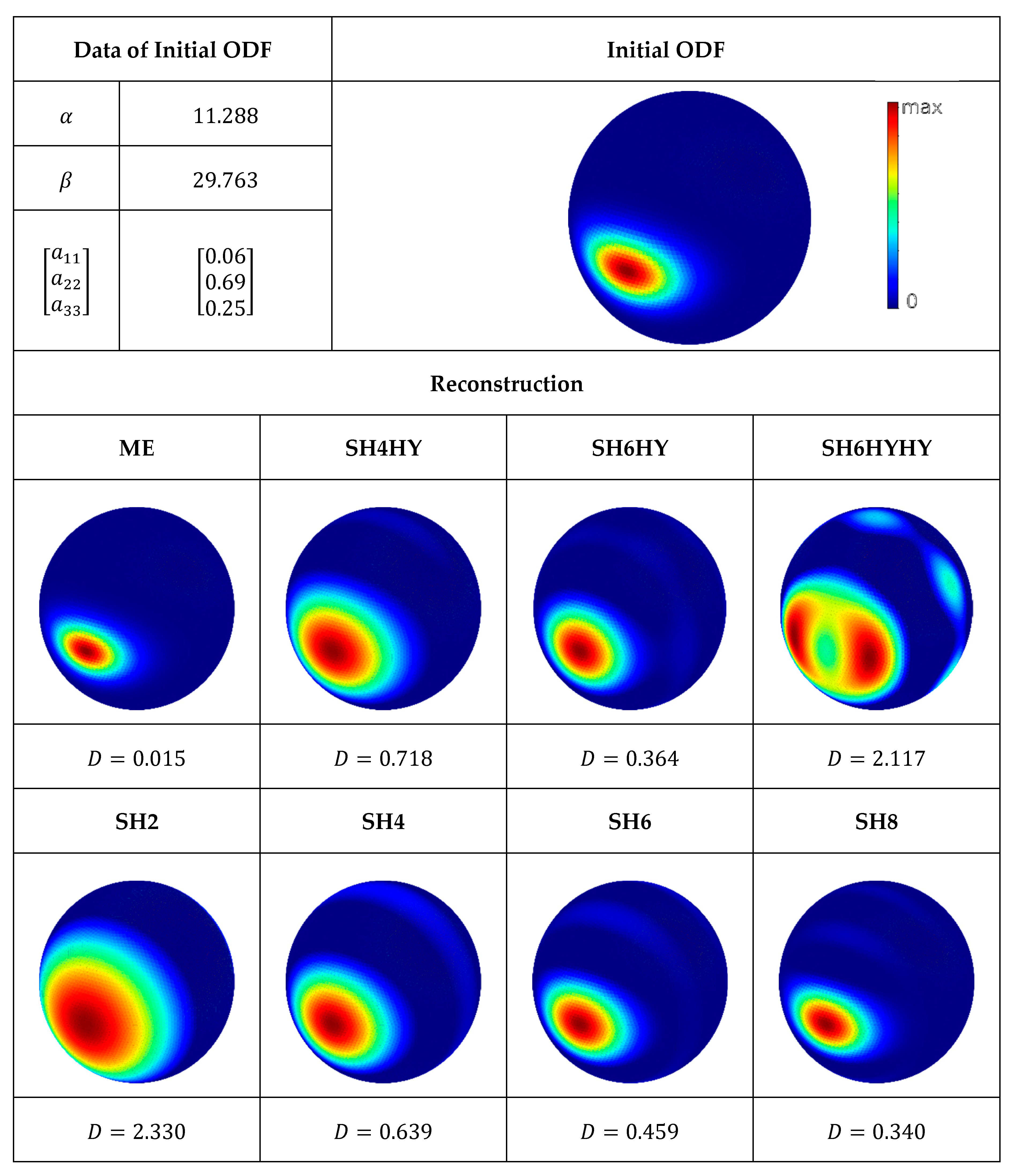
The next test scenario is given in
Figure 5 with a distribution that is similar to the first test scenario, but with a broader scattering width. The reconstruction using ME provides again an almost identical ODF compared with the initial ODF. The reconstructions SH2 and SH4 show again a larger scattering than the initial ODF. Only for SH6 and SH8 are the moments sufficient to reproduce the distribution close enough. Like in the first test scenario, secondary maxima are also recognizable by all spherical harmonic reconstructions except SH2. The SH4HY and SH6HY reconstructions are very similar to the SH4 and SH6 reconstructions, as the hybrid closure is performing well in this case. By contrast, the reconstruction SH6HYHY differs strongly from the test scenario. Both the scattering range and the secondary maximum are much more pronounced. In addition, the expected value is distributed symmetrically to two points in relation to the expected value of the test scenario. The consecutive application of hybrid closure is therefore not suitable in this case.
Figure 6 represents the next test scenario in comparison to the corresponding reconstructions. The ODF of this test scenario is characterized by a sharply limited distribution in the meridian plane, where the value at the pole positions is zero. The ME again provides the best reconstruction, where only the values of the ODF from pole to equator are slightly different. The sharp definition of the initial ODF at the poles of this test scenario is reconstructed more diffusely. The reconstructions SH2 to SH8 deliver, as expected, a too-broad ODF due to the too-few moments of spectral approximation. The secondary maxima are more pronounced in this test scenario than in the previous ones. In this test scenario, the effect of using the hybrid closure to calculate the higher tensors is particularly interesting. The reconstruction SH4HY shows two equal maxima, which are symmetrically arranged to the equatorial plane. Nevertheless, the Kullback–Leibner distance with
is approximately equal to the Kullback–Leibner distance of the reconstruction SH4. The reconstruction SH4HY illustrates the problems of using closures. Assumptions or, generally speaking, the applicability of a closure, cannot be supposed to be true in a reconstruction problem, since no information about the original ODF is known. Accordingly, the use of closures can be doubtful for the reconstruction, although higher moments are used which should be beneficial for sharply limited ODFs.
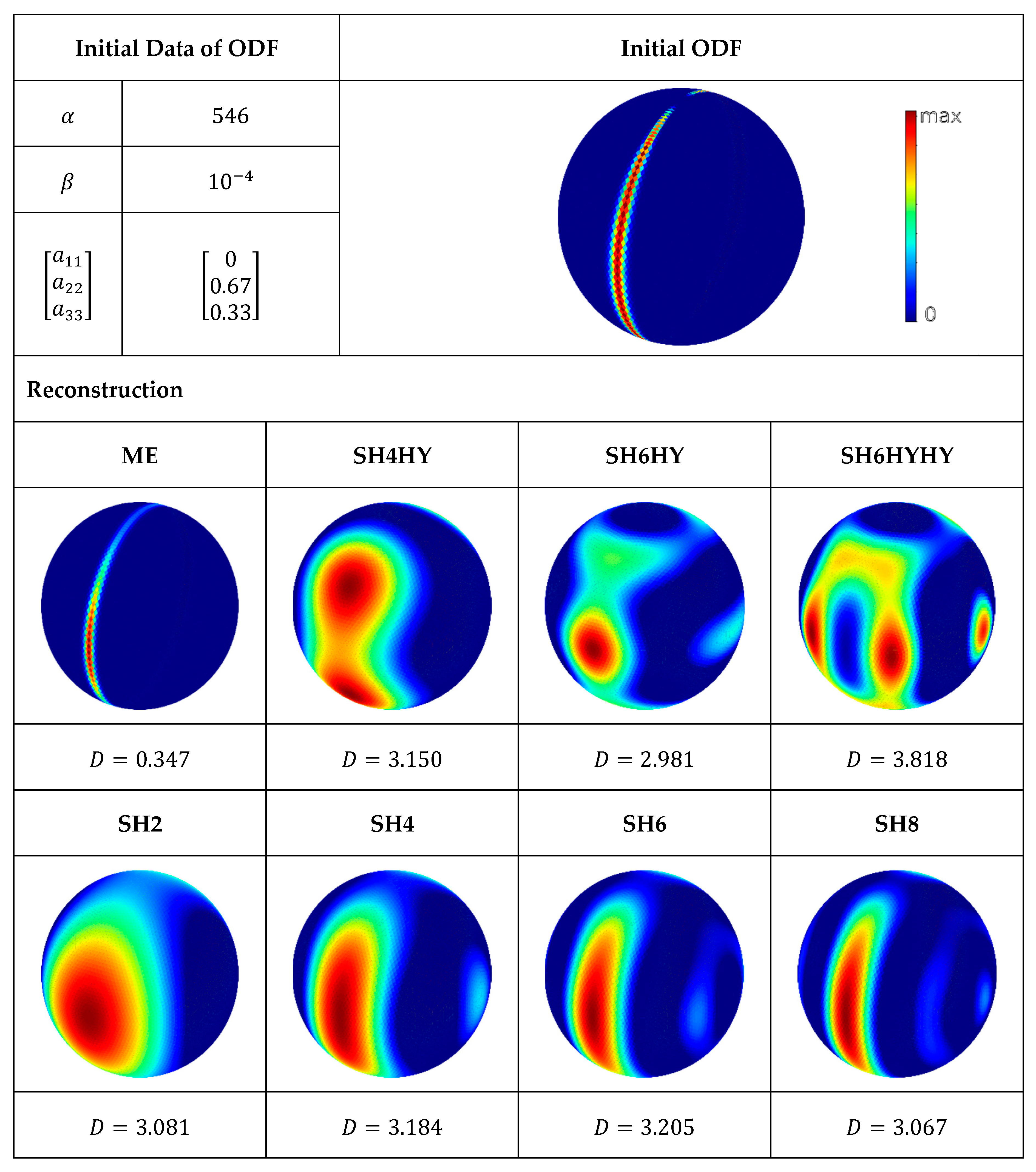
The fourth test scenario is shown in
Figure 7. The distribution is relatively broad in the meridian plane as well as over the circumference. At the poles, however, an extremely sharp border results from the fact that the even distribution on the meridian planes is diminishing as they are getting closer to each other. In contrast to the previous test procedures, the ME method appears not to be the best solution, as it does not provide sharp distribution at the poles. In the reconstructions SH4 to SH8, several maxima can be observed, which merge more and more together as the number of moments increases.
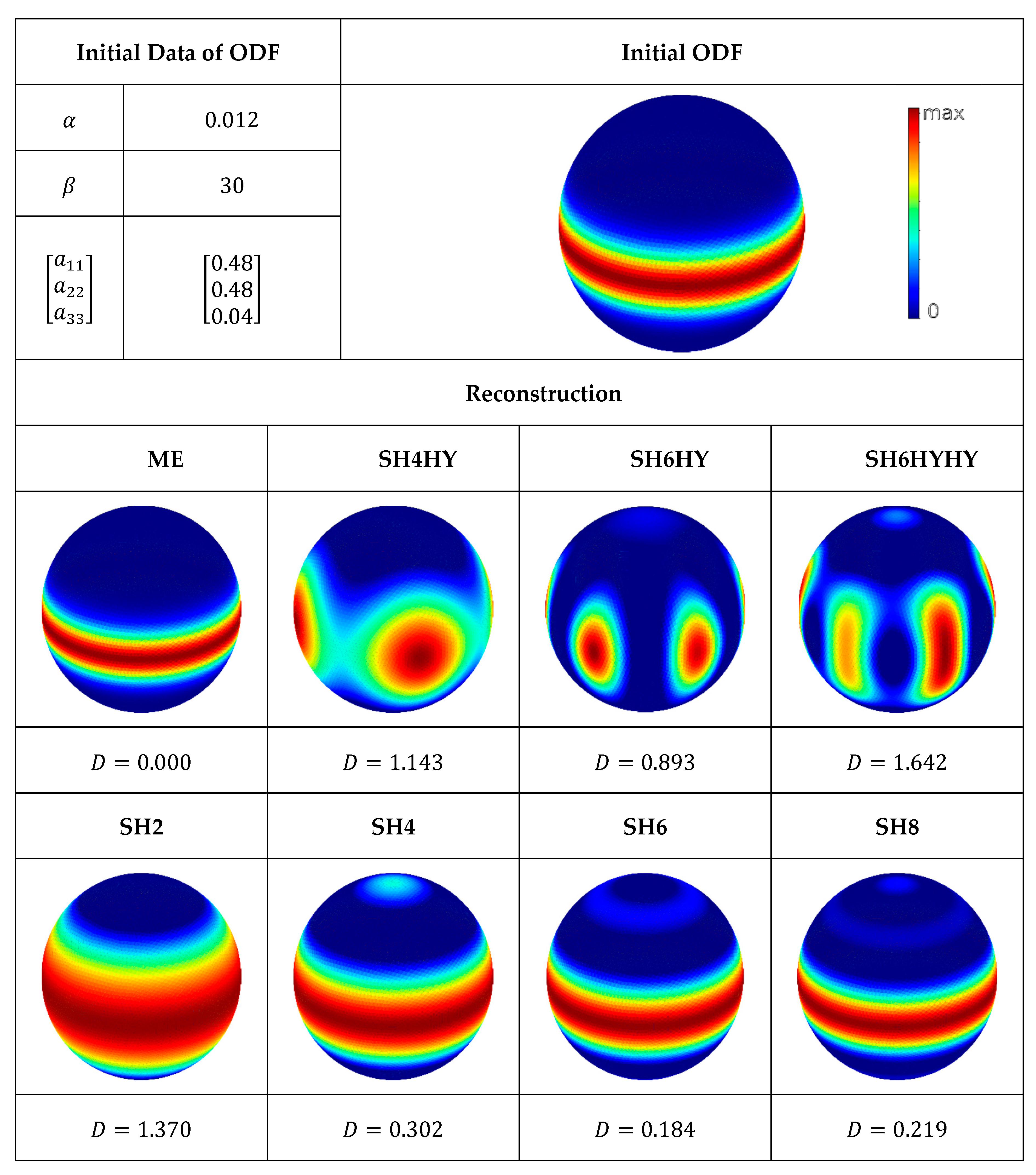
The last example of test scenarios shows a relatively broad, almost circumferential distribution on the equatorial plane (see
Figure 8). The reconstruction using ME is exact. Once again, the reconstruction using hybrid closure is questionable. Several maxima occur in the reconstructions SH4HY, SH6HY, and SH6HYHY and are much more pronounced than in the previous test scenarios. Furthermore, the Kullback–Leibner distance is significantly worse compared to the reconstructions SH4 and SH6.
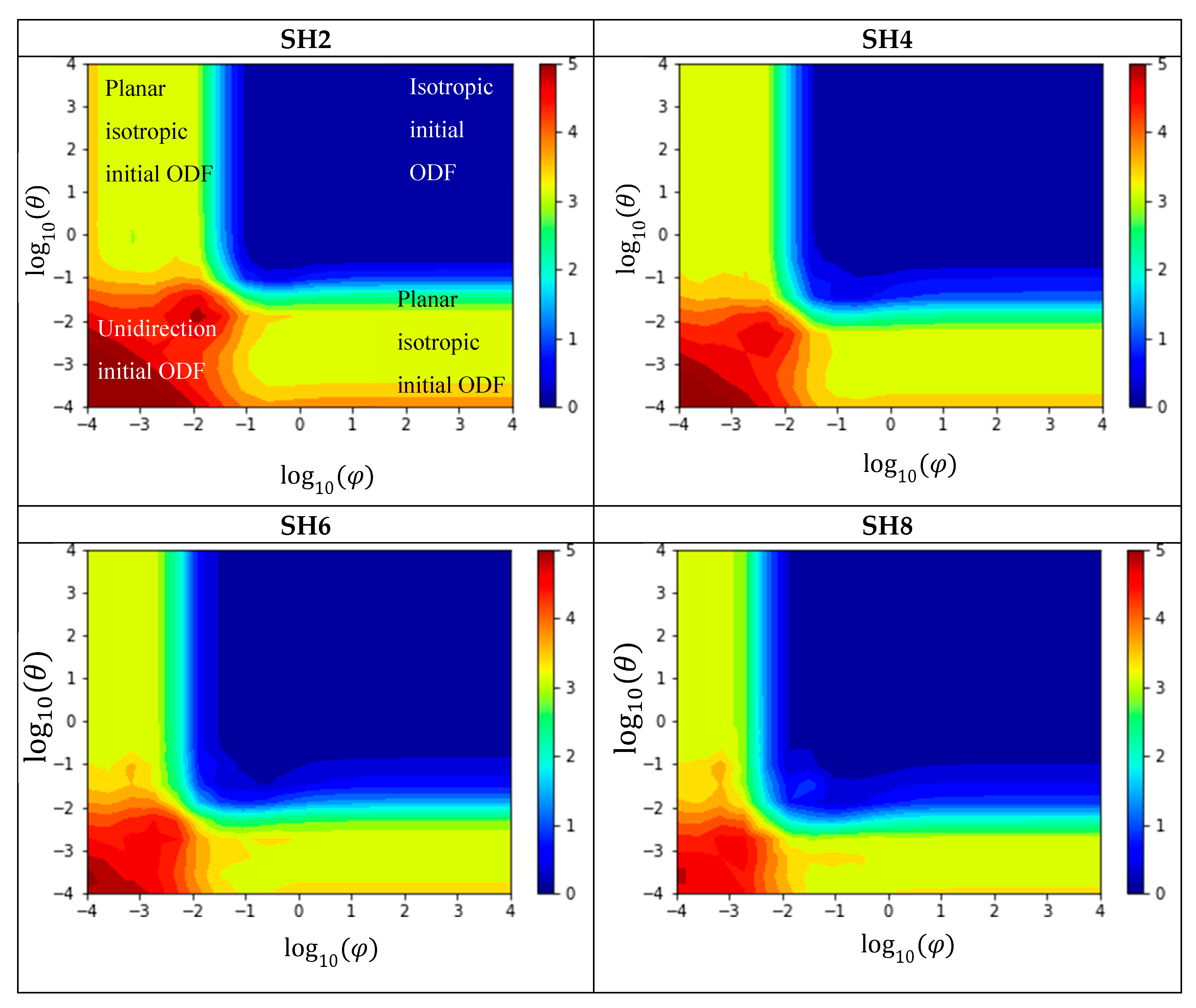
In the following, all test scenarios for the evaluation of the reconstruction methods are compared against each other. First, the methods SH2 to SH8 are analyzed. The Kullback–Leibner distance as a function of the logarithmically covariances
and
is shown in
Figure 9. The value of the Kullback–Leibner distance is represented by a color. The figure shows that the reconstruction methods SH2 to SH8 are qualitatively very similar. In the range of nearly unidirectional initial fiber orientation, the Kullback–Leibner distance is large, whereas in the range of isotropic initial fiber orientation, the Kullback–Leibner distance is nearly zero. As the number of moments increases, the Kullback–Leibner distance becomes smaller, but still not significant.
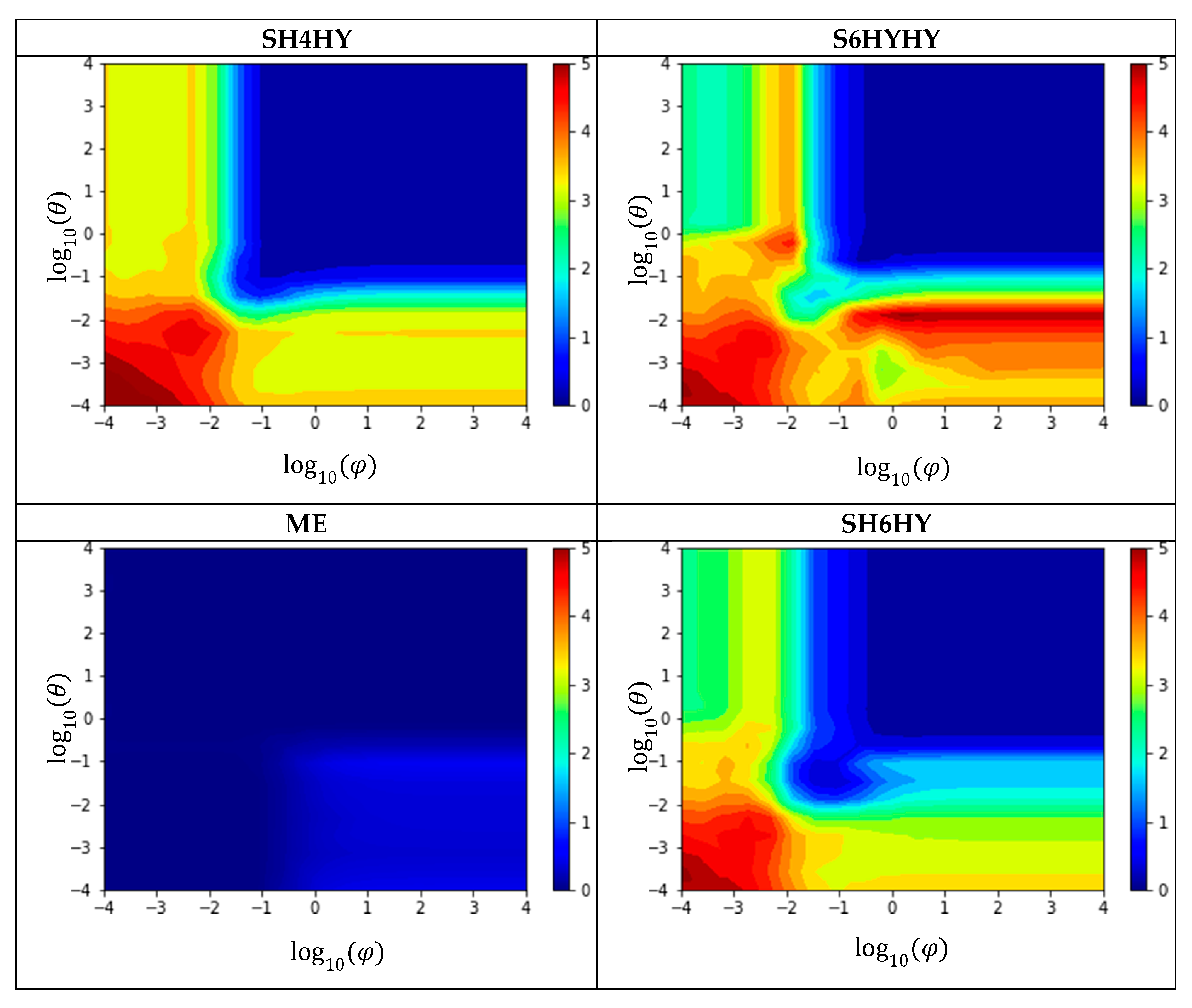
The reconstructions SH4HY, SH6HY, and SH6HYHY, shown in
Figure 10, differ essentially from SH4 and SH6 in cases where one of the covariances is small and the other large. In these cases, the Kullback–Leibner distance is either greater or smaller. Especially in SH6HYHY reconstructions, both cases occur simultaneously. The evaluation of the Kullback–Leibner distance in SH4HY, SH6HY, and SH6HYHY is no longer symmetrical to the bisector. An exact explanation of the differences with hybrid closure is therefore accordingly difficult. It is known that the hybrid closure overestimates the fiber alignment. This is counteracted by a too-low order of moment used. The shown comparison is designed in such a way that the methods SH2 to SH8 get the exact tensors of higher order and should therefore have a lower Kullback–Leibner distance. The supposed improvement of the Kullback–Leibner distance using the hybrid closure is therefore not to be regarded as an improvement as such, but rather as more or less random, as the overprediction of alignment equalizes the too-low order of moments.
The reconstruction with ME shows a consistently low Kullback–Leibner distance. This proves that the maximum entropy method is capable of reconstructing a distribution function so far as all information is contained in the fiber orientation tensor. This is the case in the example of the Bingham distribution chosen here, since the expected value is clearly determined by the eigenvectors of the second-order fiber orientation tensor, and the scatter can be determined from the eigenvalues.
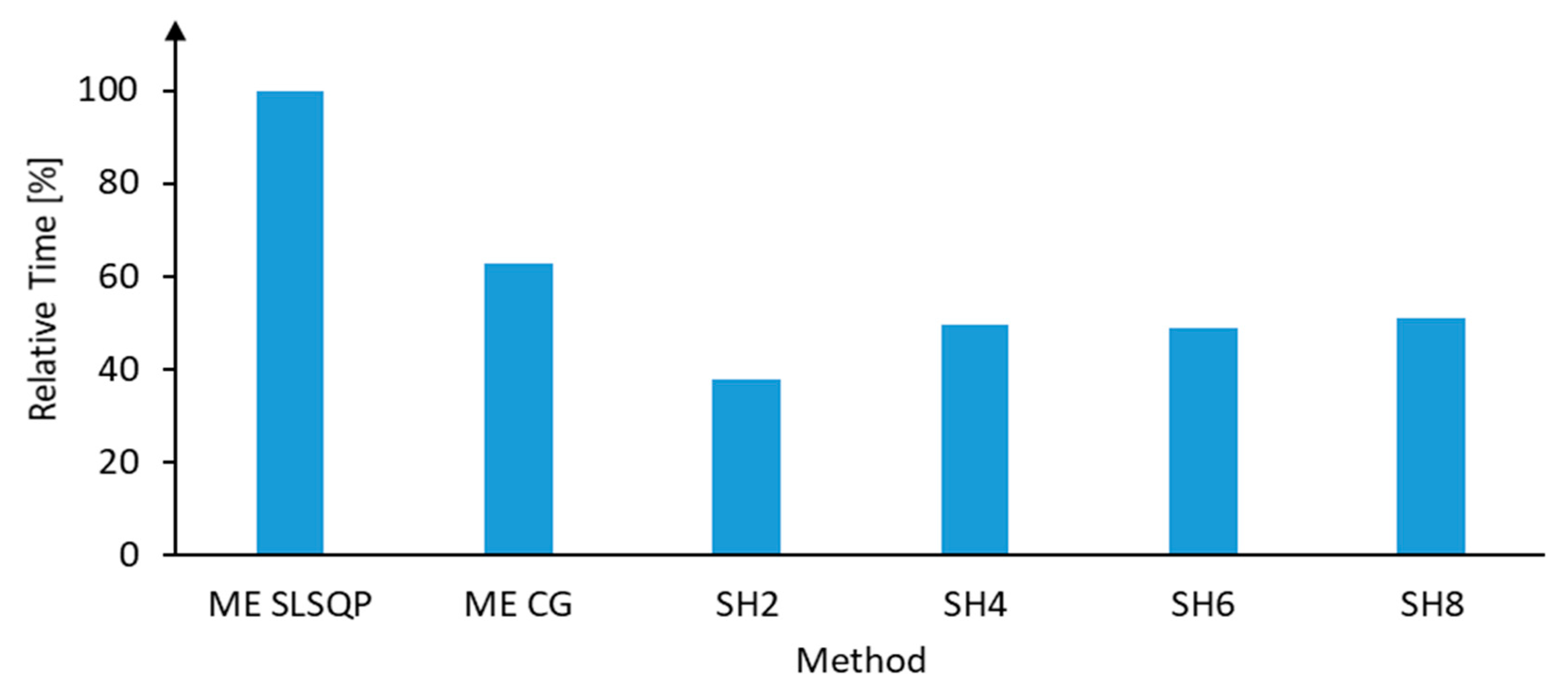
In the context of a reconstruction problem, the quality of the reconstruction as well as the computing time is of interest.
Figure 11 shows the time required to perform a reconstruction. The indicated time refers exclusively to the reconstruction, i.e., the calculation of the fiber orientation tensors of the initial ODF is not considered. The performed benchmark is implemented in the programming language Python, whereby each reconstruction method is vectorized and sped up as far as possible. The benchmark is performed on an AMD Ryzen 7 1800X system (Advanced Micro Devices, Inc., Santa Clara, CA, USA). As already mentioned, the influence of the numerical method of the ME method on the required computing time is analyzed. Note that due to the specified tolerance, the reconstruction is identical for both numerical methods.
In
Figure 11, the time is given relative to ME SLQP, which on average takes 1.29 s. It turns out that the SH2 method is the fastest. SH4 to SH8 are about 30% slower, although interestingly, there is no significant difference between SH4, SH6, and SH8. The ME method with the CG algorithm is about 65% slower than the SH2 method. With the SLSQP algorithm, the ME method is considerably slower than with the CG algorithm.
5.4. Numerical Results for Measured Data
In addition to the synthetic benchmarks in
Section 5.3, measured fiber orientation was used for comparison. These data originate exclusively from the literature.
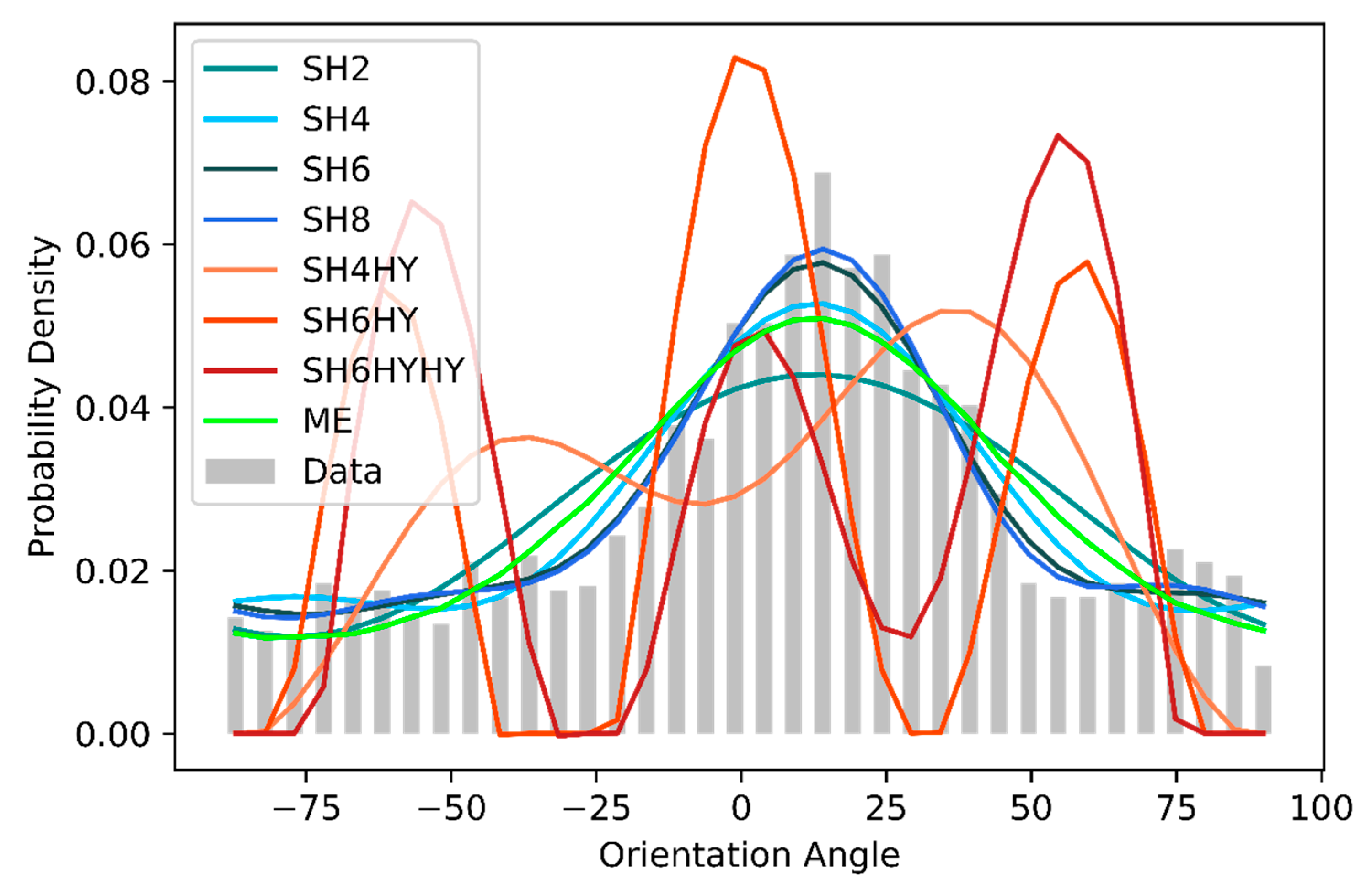
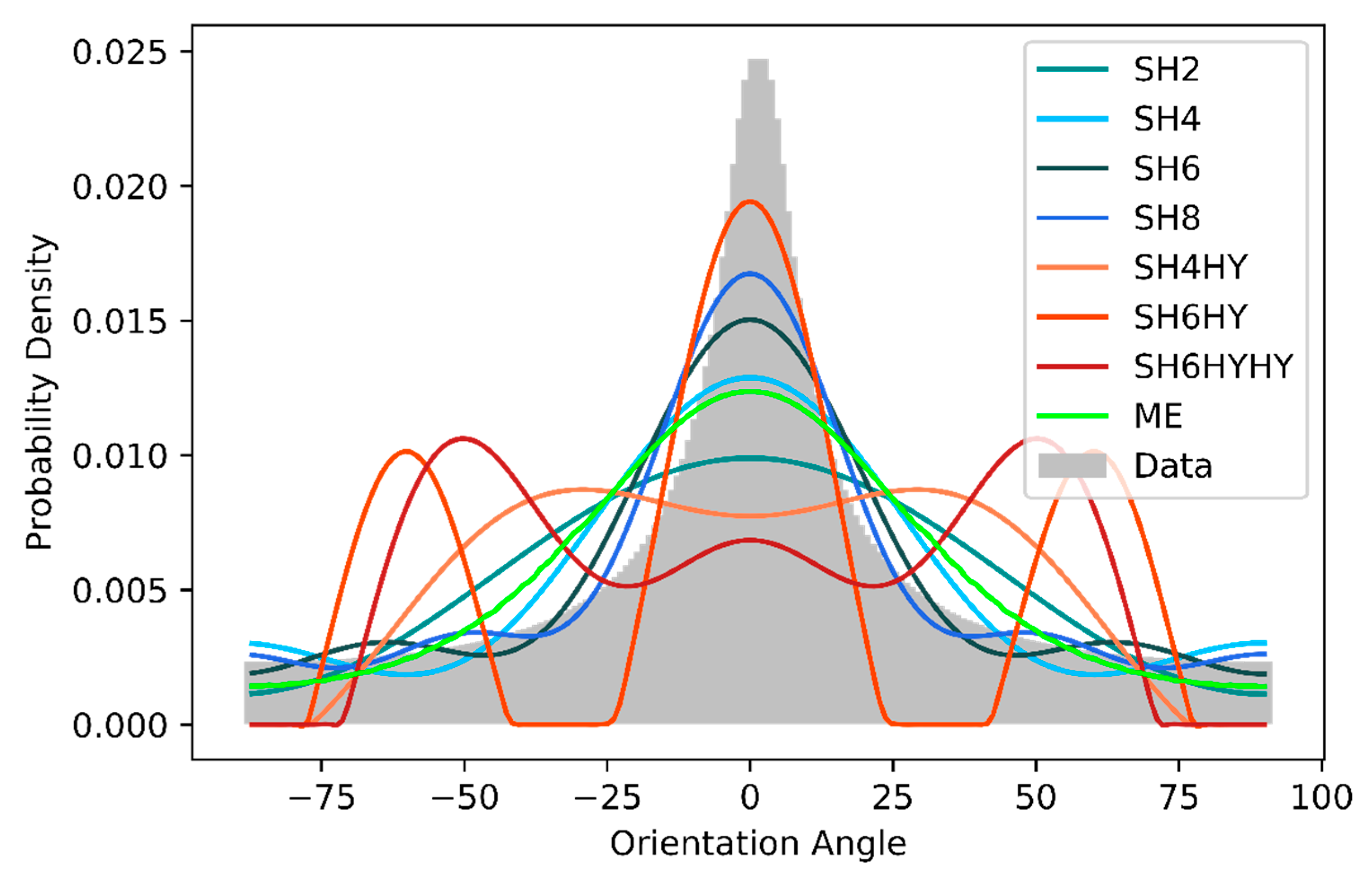
The first set of data was taken from [
7] and is shown in
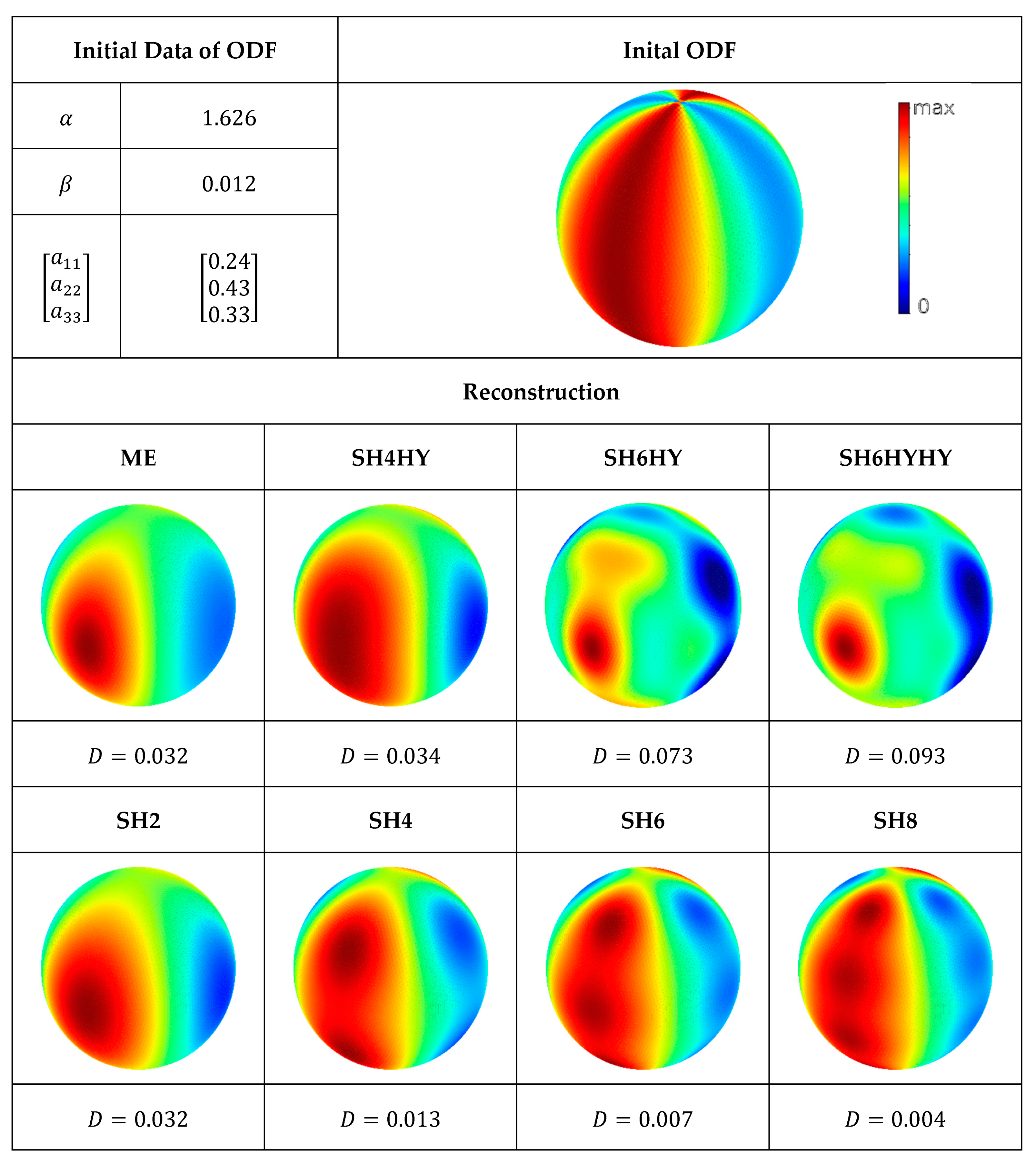
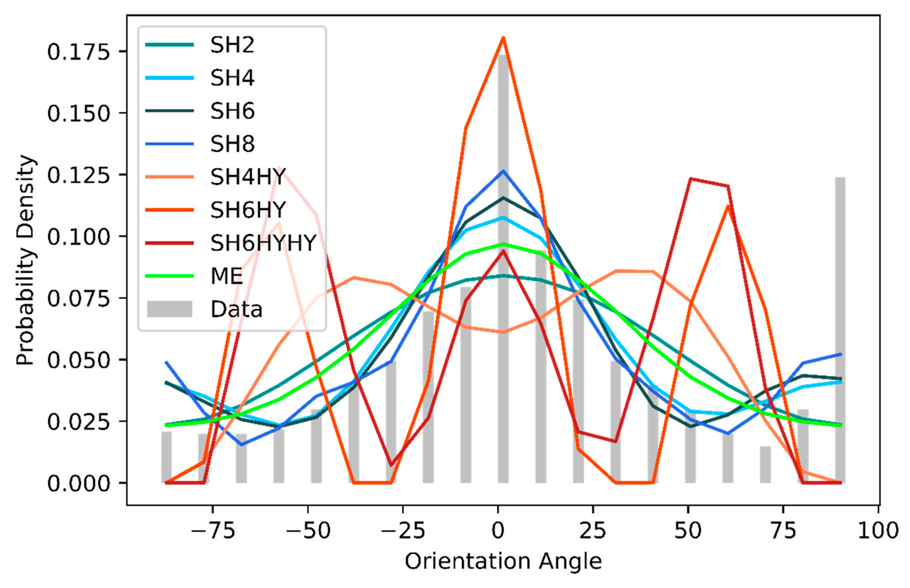
Figure 12 together with the reconstructions. The methods SH2 to SH8 can reconstruct the data relatively well, whereby the absolute height at the expected value is clearly underestimated, especially for SH2 and SH4. The scatter of the reconstructions is wider than the original ODF. The reason for that was already discussed for the Bingham test scenarios: The number of moments used is too low to be able to represent the peak. The reconstructions based on the hybrid closure again show a completely different behavior. Several maximum values are reconstructed, as well as a shift of the expected value. The ME method reconstructs the ODF relatively well, although with a too-low probability density around the maximum of the initial ODF and a too-wide scattering, especially at −30° and +50°.
The second set of data was taken from [
43]. The fiber orientation was measured by μComputer Tomography (µCT) of injection molded samples. Subsequently, the ODF was subdivided into shell and core layers, with the shell layer used here. In this dataset, the peak at 90° is particularly interesting in respect of to what extent it can be reconstructed (see
Figure 13). In the area around the expected value, the behavior is basically similar to that of the first set of data. The methods SH2 to SH8 and ME underestimate the absolute value at the expected value. With SH2 and ME, the reconstructed probability at ±50° is again too high, and the peak at 90° cannot be reconstructed. Here, only the methods SH4, SH6, and SH8 can generate something that is similar to a second peak. The reconstruction methods with hybrid closure reconstruct several maxima symmetrically to the expected value again.
The third ODF was taken out of Lenke [
44]. In this case, however, the direct numerical values of the μCT-experimentally-measured ODF were not used, but a probability density function that represents the measured data in an extremely good approximation. The probability density function is described in Lenke’s work by:
The reconstruction of the methods is exactly analogous to the previous examples.
Figure 14 shows the results. The methods SH2 to SH8 become better with each increasing moment to reconstruct the ODF. Here, an oscillation is very noticeable apart from the expected value. The reconstructions with hybrid closures generate several maxima again. In addition to that, it becomes evident that the ME method does not work well enough here, because the original ODF is not a Bingham distribution.
6. Conclusions
The aim of this work was to compare and evaluate existing reconstruction methods of a fiber orientation distribution based on fiber orientation tensors. The evaluation was based on the Kullback–Leibner distance as well as on a direct qualitative comparison of the obtained distributions.
In a first step, initial ODFs were generated and the related fiber orientation tensors were determined. Using reconstruction methods, the approximated ODF was calculated on the basis of the fiber orientation tensors. The initial ODFs generated were of a Bingham distribution type, and experimentally measured data from the literature were also used.
None of the investigated reconstruction methods can be considered as the best in general. Although the maximum entropy method impressively shows that a certain distribution can be reconstructed almost identically, this is only if the distribution type is of the same type. The Bingham distribution chosen in this paper was practically reconstructed one-to-one by the maximum entropy method. In the reconstruction of the measured data, however, the weakness of the maximum entropy method becomes apparent: Distributions different from a Bingham distribution or outliers cannot be reconstructed. This is a strength of the spectral harmonics approximations, which in principle could represent any distribution function. Nevertheless, this reconstruction method cannot be considered ideal either, since the moments in particular must be correspondingly high in order to be able to map certain distribution functions. It has been shown that even with the fiber orientation tensor of the eighth order included, sharply limited distributions cannot be reconstructed. Moreover, these high moments are usually not available in process simulations. Although closures offer the possibility of higher moments, however, the problem here are the closures themselves, since assumptions have to be made about the distribution function.
With the mentioned advantages and disadvantages of both reconstruction methods, it can be concluded that in the case of the reconstruction of an ODF only on the basis of a second-order fiber orientation tensor without any further information about the ODF, the maximum entropy method seems to be on average the best choice. This is evident from the following two reasons: Firstly, the assumption of maximum entropy is a physical approach, which Hine et al. [
36] can largely confirm with experimentally measured fiber orientations. Secondly, the reconstructions in this contribution show that the errors of the maximum entropy method are much smaller than those of the frequently used SH4HY method (spherical harmonics, 4th order, with hybrid closure).


