Kinematic Fields Measurement during Orthogonal Cutting Using Digital Images Correlation: A Review


Abstract
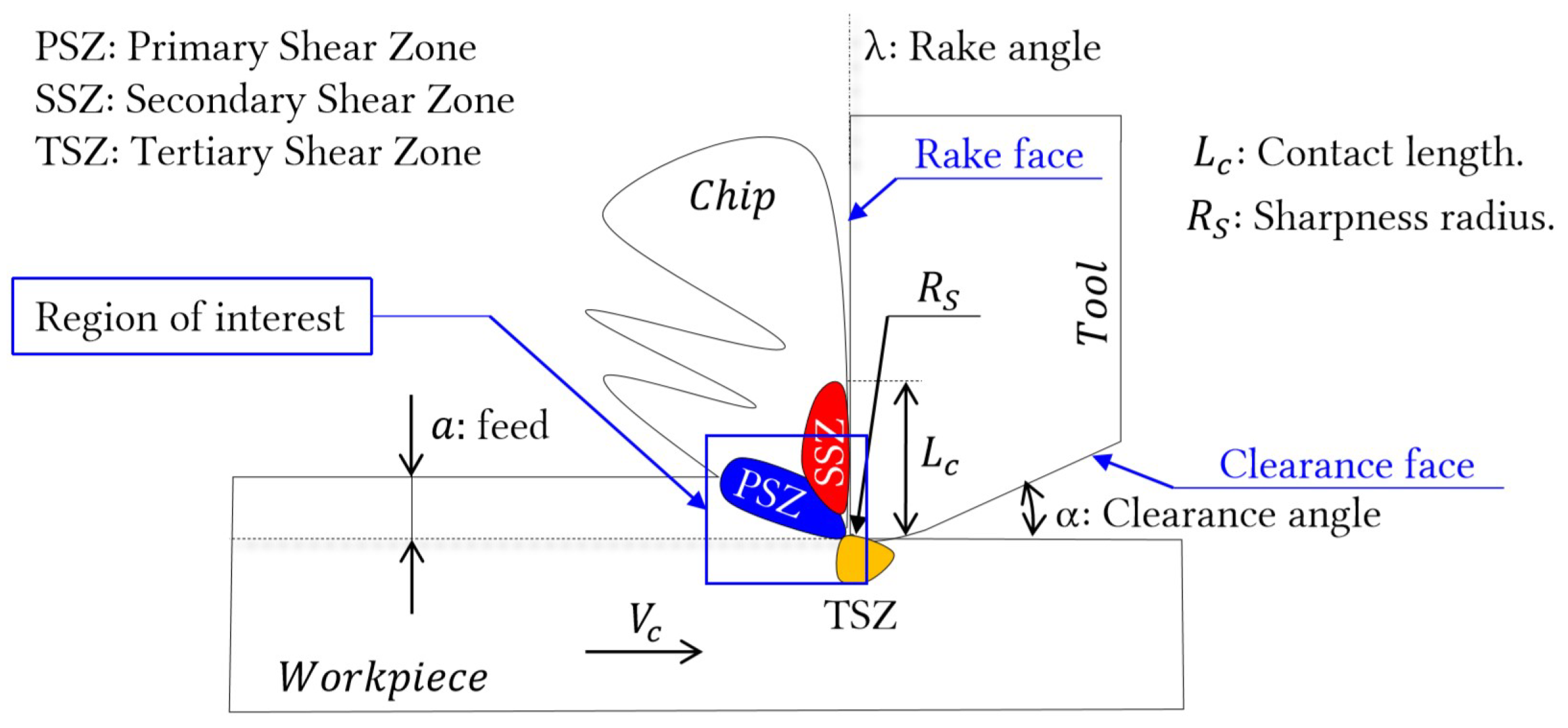
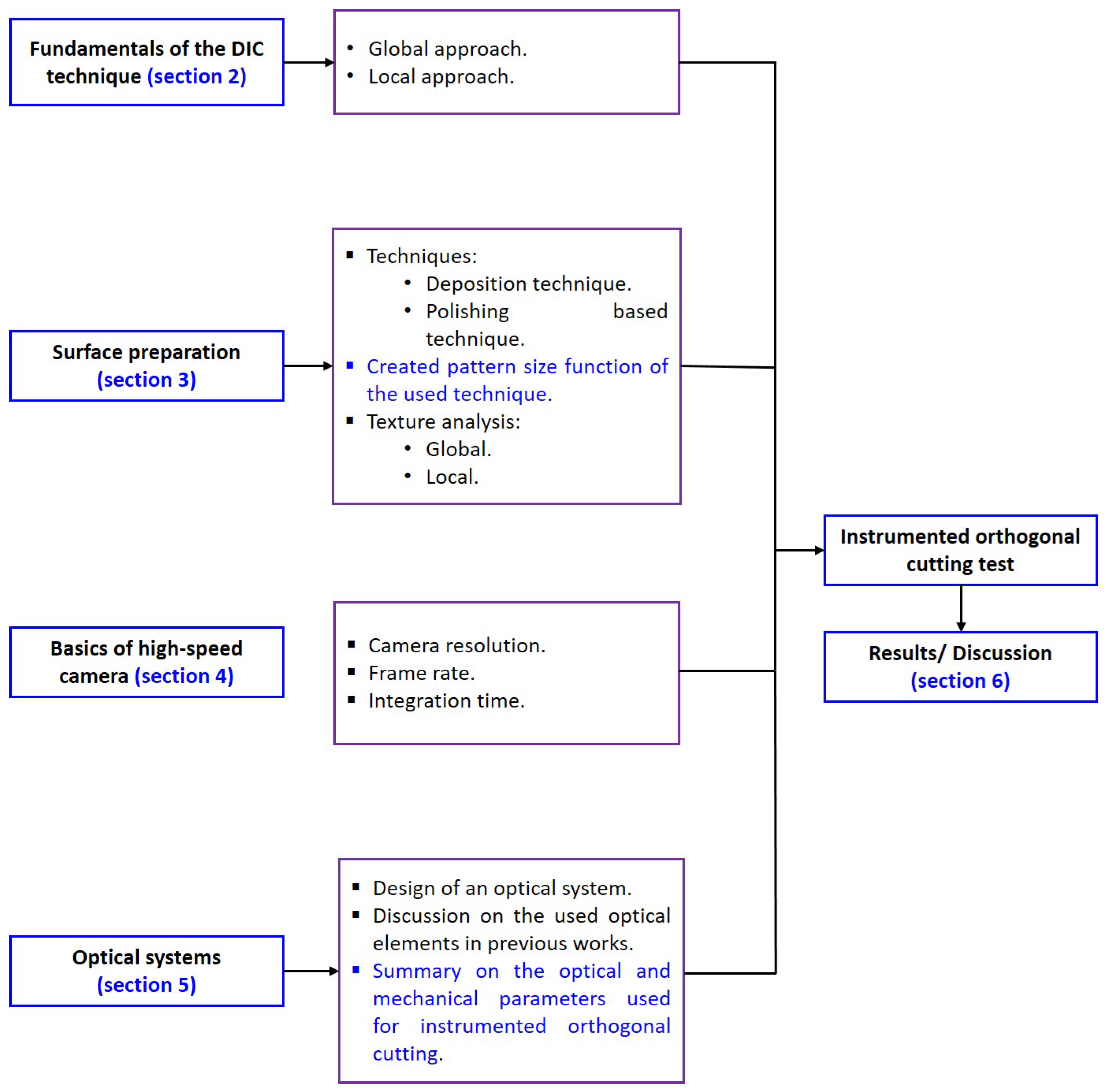
1. Introduction
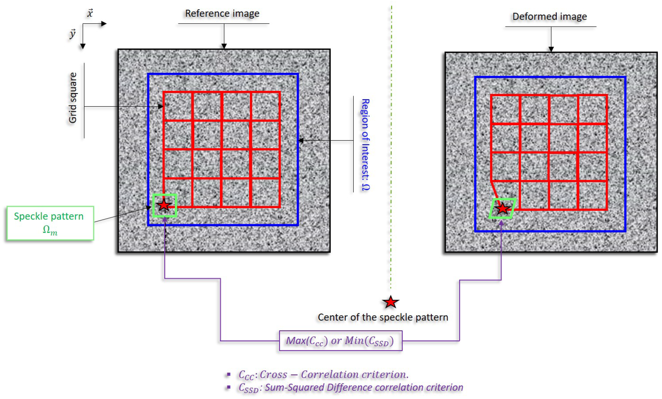
2. Fundamentals of the DIC Technique
2.1. Global Approach
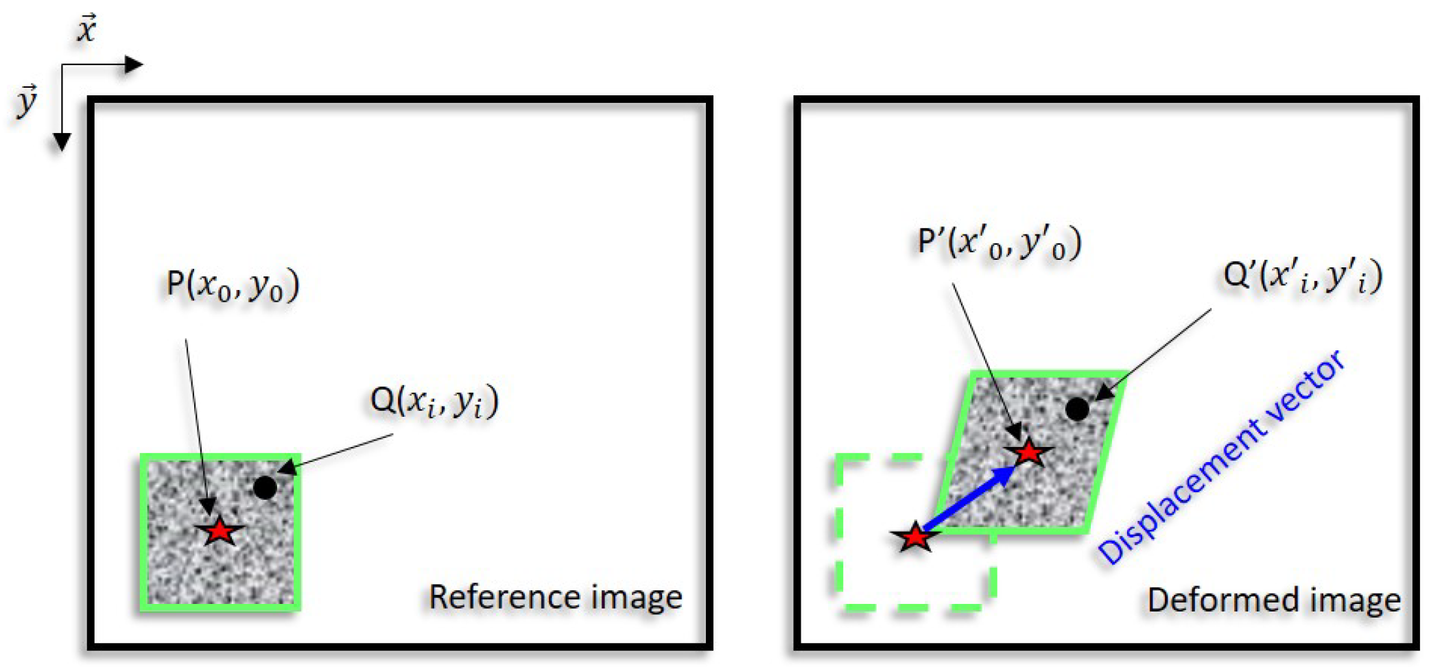
2.2. Local Approach
3. Surface Preparation of the Workpiece for DIC Post-Processing
3.1. Techniques
3.1.1. Deposition Technique
3.1.2. “Polishing Based” Technique
- the grid square size when using the grid technique (Gr) for the surface preparation;
- the lines spacing when using the flow lines scratching technique; and,
- the speckle pattern size when using the deposition or the “polishing based” technique.
3.1.3. Discussion/Comparison
3.2. Texture Analysis
3.2.1. Global Analysis
- the degree of the image’s luminosity; and,
- the grey level dynamic of the image (N), where:and are respectively the maximum and the minimum grey levels.
3.2.2. Local Analysis
- Mean Gray Level Fluctuation
- Autocorrelation function
- Mean Intensity Gradient (MIG)
- Rigid body motion approach
4. Basics of High-Speed Camera
4.1. Camera Resolution
4.2. Frame Rate
4.3. Integration Time
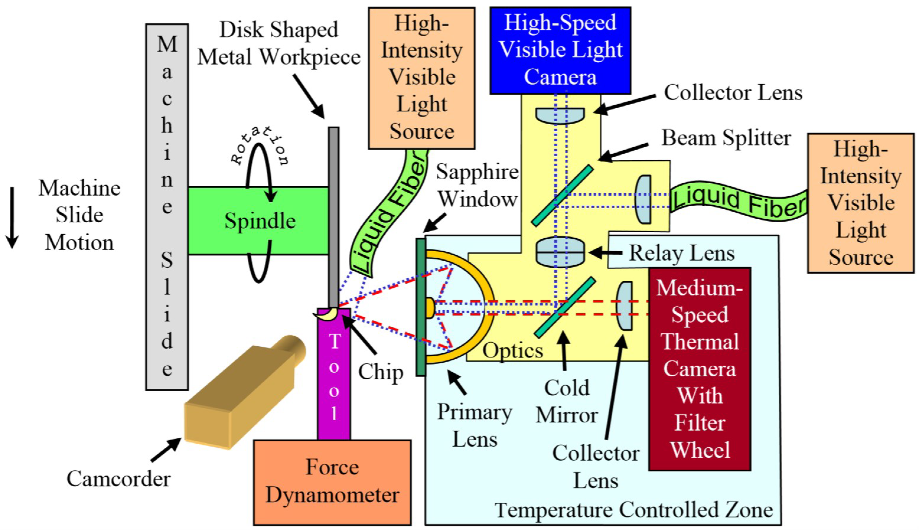
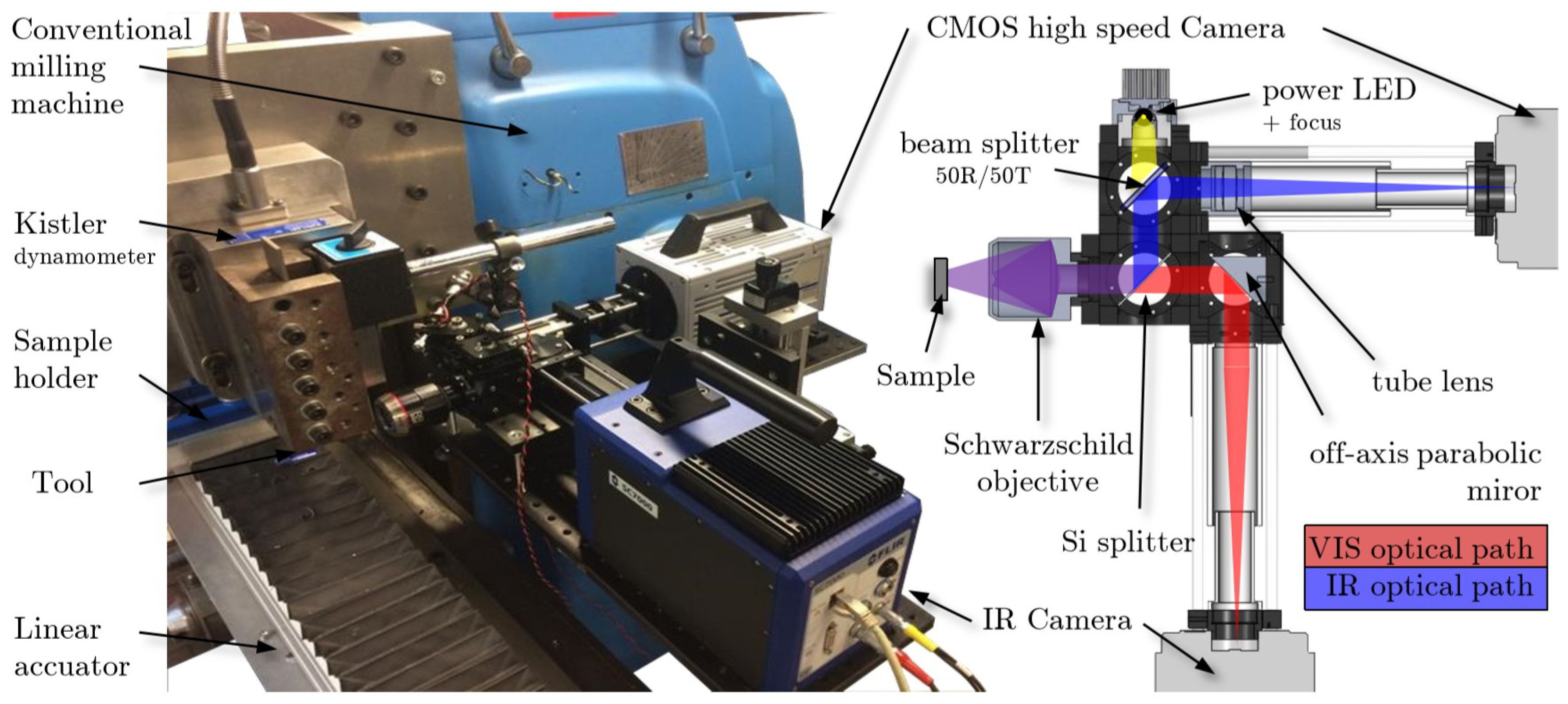
5. Optical Systems
6. Results/Discussion
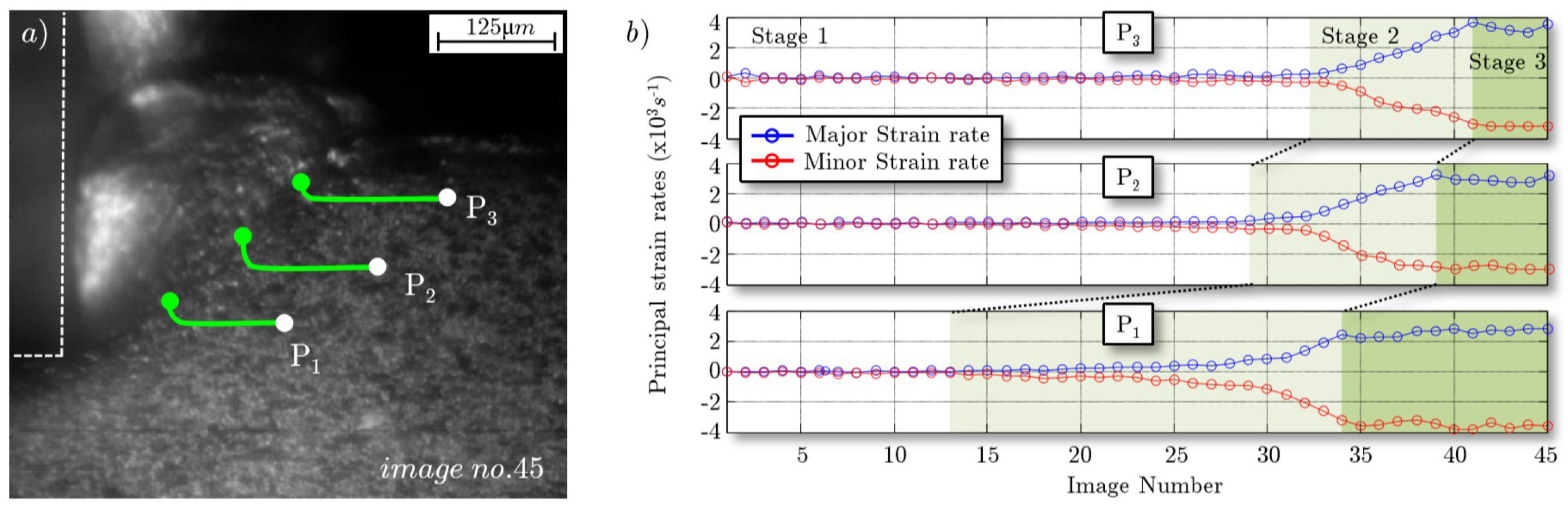
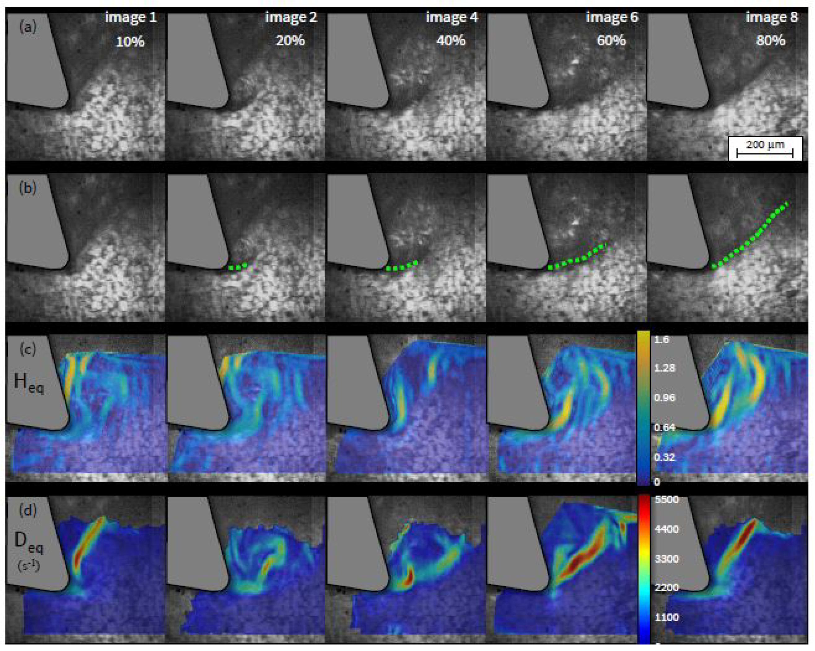
- stage 1: strain concentration at the tool-tip vicinity.
- stage 2: rapid strain accumulation within the ASB from the tool tip to the free surface. The strain rate magnitude is up to 4 × s and leads to a material failure.
- stage 3: the strain rate became stable and the segment chip is fully formed.
- for Al7075-T651 and with low cutting speed, the plastic strain magnitude is ranging from 1 to 2 with a strain rate magnitude of 10 s [54];
- for nickel based alloy and with a cutting speed of 30 m/min (respectively 150 m/min.), the plastic strain magnitude is ranging from 1.2 to 1.4 with a strain rate magnitude of 10 s (respectively 10 s) [57].
7. Conclusions
- in-situ investigation of the material flow during machining requires surface preparation of the workpiece. Various techniques of surface preparation were discussed and classified in term of created pattern size. It was found that the “polishing based” technique is the most suitable for kinematic fields measurement in orthogonal cutting. It offers an acceptable pattern size sufficient enough to identify high localized deformation band. The speckle pattern size is identified through texture analysis. Various texture analysis tools were discussed. The MIG aproach and rigid body motion approach prove to be the most reliable tools in evaluating the property of the DIC application.
- With the development of high-speed cameras, significant progress on the kinematic fields measurement has been made. The basics of high-speed camera were discussed and yield a definition of a methodology that can be followed to determine the optimum optical parameters.
- With the recent advances on the design of optical systems, real-time insight on the material flow during orthogonal cutting through surface observation of the PSZ was made possible. Captured images with sufficient quality can be obtained allowing for a proper application of the DIC technique.
- Details on the used two approaches (global and local) with the DIC technique were presented. The choice of the appropriate correlation criterion is important. It was found that the ZNCC (Zero-Normalized Cross Correlation) and the ZNSSD (Zero-Normalized Sum of Squared Differences) correlation criteria are the most suitable, due to the fact that both criteria are insensitive to a scale in lighting. Because of the loss of image quality, the incremental correlation type is priviliged for the kinematic fields measurement during orthogonal cutting.
- During orthogonal cutting, the material undergones translation, rotation, and shear. Thus, minimum first-order shape functions are required for the displacement fields interpolation.
Author Contributions
Funding
Conflicts of Interest
References
- Jaspers, S.P.F.C.; Dautzenberg, J.H. Material behaviour in metal cutting: Strains, strain rates and temperatures in chip formation. J. Mater. Process. Technol. 2002, 121, 123–135. [Google Scholar] [CrossRef]
- Germain, G.; Morel, A.; Braham-Bouchnak, T. Identification of Material Constitutive Laws Representative of Machining Conditions for Two Titanium Alloys: Ti6Al4V and Ti555-3. J. Eng. Mater. Technol. 2013, 135, 031002. [Google Scholar] [CrossRef]
- Liu, R.; Melkote, S.; Pucha, R.; Morehouse, J.; Man, X.; Marusich, T. An enhanced constitutive material model for machining of Ti–6Al–4V alloy. J. Mater. Process. Technol. 2013, 213, 2238–2246. [Google Scholar] [CrossRef]
- Johnson, G.R.; Cook, W.H. A constitutive model and data for materials subjected to large strains, high strain rates, and high temperatures. Proc. Seventh Int. Symp. Ballist. 1983, 21, 541–547. [Google Scholar]
- Calamaz, M.; Coupard, D.; Girot, F. Numerical simulation of titanium alloy dry machining with a strain softening constitutive law. Mach. Sci. Technol. 2010, 14, 244–257. [Google Scholar] [CrossRef]
- Sima, M.; Ozel, T. Modified material constitutive models for serrated chip formation simulations and experimental validation in machining of titanium alloy Ti–6Al–4V. Int. J. Mach. Tools Manuf. 2010, 50, 943–960. [Google Scholar] [CrossRef]
- List, G. Etude des méCanismes D’endommagement des Outils Carbure WC-Co par la CaractéRisation de L’interface Outil Copeau: Application à L’usinage à sec de L’alliage D’aluminium Aéronautique AA2024 T351. Ph.D. Thesis, ENSAM de Bordeaux, Paris, France, 2010. [Google Scholar]
- Bahi, S. Modélisation Hybride du Frottement Local à L’interface Outil-Copeau en Usinage des Alliages Métalliques. Ph.D. Thesis, ENSAM de Bordeaux, Paris, France, 2004. [Google Scholar]
- Atlati, S.; Haddag, B.; Zenasni, M. Thermomechanical modelling of the tool–workmaterial interface in machining and its implementation using the ABAQUS VUINTER subroutine. Int. J. Mech. Sci. 2014, 87, 102–117. [Google Scholar] [CrossRef]
- Mabrouki, T.; Girardin, F.; Asad, M.; Rigal, J.F. Numerical and experimental study of dry cutting for an aeronautic aluminium alloy (A2024-T351). Int. J. Mach. Tools Manuf. 2008, 48, 1187–1197. [Google Scholar] [CrossRef]
- Karpat, Y. Temperature dependent flow softening of titanium alloy Ti6Al4V: An investigation using finite element simulation of machining. J. Mater. Process. Technol. 2011, 211, 737–749. [Google Scholar] [CrossRef]
- Huang, Y.; Ji, J.; Lee, K.M. An improved material constitutive model considering temperature-dependent dynamic recrystallization for numerical analysis of Ti-6Al-4V alloy machining. Int. J. Adv. Manuf. Technol. 2018, 97, 3655–3670. [Google Scholar] [CrossRef]
- Harzallah, M.; Pottier, T.; Senatore, J.; Mousseigne, M.; Germain, G.; Landon, Y. Numerical and experimental investigations of Ti-6Al-4V chip generation and thermo-mechanical couplings in orthogonal cutting. Int. J. Mech. Sci. 2017, 134, 189–202. [Google Scholar] [CrossRef]
- Courbon, C. Vers une Modélisation Physique de la Coupe des Aciers Spéciaux: Intégration du Comportement Métallurgique et des Phénomènes Tribologiques et Thermiques aux Interfaces. Ph.D. Thesis, Ecole Centrale de Lyon, Lyon, France, 2011. [Google Scholar]
- Rotella, G.; Dillon, O.W., Jr.; Umbrello, D.; Settineri, L.; Jawahir, I.S. Finite element modeling of microstructural changes in turning of AA7075-T651 Alloy. J. Manuf. Process. 2013, 15, 87–95. [Google Scholar] [CrossRef]
- Jafarian, F.; Imaz Ciaran, M.; Umbrello, D.; Arrazola, P.J.; Filice, L.; Amirabadi, H. Finite element simulation of machining Inconel 718 alloy including microstructure changes. Int. J. Mech. Sci. 2014, 88, 110–121. [Google Scholar] [CrossRef]
- Wang, Q.; Liu, Z.; Wang, B.; Song, Q.; Wan, Y. Evolutions of grain size and micro-hardness during chip formation and machined surface generation for Ti-6Al-4V in high-speed machining. Int. J. Adv. Manuf. Technol. 2015, 82, 1725–1736. [Google Scholar] [CrossRef]
- Wagner, V.; Barelli, F.; Dessein, G.; Laheurte, R.; Darnis, P.; Cahuc, O.; Mousseigne, M. Comparison of the chip formations during turning of Ti64 beta and Ti64 alpha+beta. J. Eng. Manuf. 2019, 233, 494–504. [Google Scholar] [CrossRef]
- Barelli, F. Développement d’une Méthodologie D’optimisation des Conditions d’usinage: Application au Fraisage de l’alliage de Titane TA6V. Ph.D. Thesis, Université de Toulouse, Toulouse, France, 2016. [Google Scholar]
- Ramirez, C. Critères D’optimisation des Alliages de Titane pour Améliorer leur Usinabilité. Ph.D. Thesis, ENSAM de Cluny, Paris, France, 2017. [Google Scholar]
- Battaglia, J.; Puigsegur, L.; Cahuc, O. Estimated temperature on a machined surface using an inverse approach. Exp. Heat Transf. 2006, 18, 13–32. [Google Scholar] [CrossRef]
- Cahuc, O.; Darnis, P.; Laheurte, R. Mechanical and Thermal Experiments in Cutting Process for New Behaviour Law. Int. J. Form. Process. 2007, 10, 235–269. [Google Scholar] [CrossRef]
- Haddag, B.; Atlati, S.; Zenasni, M. Analysis of the heat transfer at the tool–workpiece interface in machining: Determination of heat generation and heat transfer coefficients. Heat Mass Transf. 2015, 51, 1355–1370. [Google Scholar] [CrossRef]
- Baizeau, T.; Campocasso, S.; Fromentin, G.; Besnard, R. Kinematic Field Measurements During Orthogonal Cutting Tests via DIC with Double-frame Camera and Pulsed Laser Lighting. Exp. Mech. 2008, 57, 581–591. [Google Scholar] [CrossRef]
- Zhang, D.; Zhang, X.M.; Leopold, J.; Ding, H. Subsurface Deformation Generated by Orthogonal Cutting: Analytical Modeling and Experimental Verification. J. Manuf. Sci. Eng. 2017, 139, 094502. [Google Scholar] [CrossRef]
- Bitans, K.; Brown, R.H. An investigation of the deformation in orthogonal cutting. Int. J. Mach. Tool Des. Res. 1965, 5, 155–165. [Google Scholar] [CrossRef]
- Brown, R.H. A double shear-pin quick-stop device for very rapid disengagement of a cutting tool. Int. J. Mach. Tool Des. Res. 1976, 16, 115–121. [Google Scholar] [CrossRef]
- Vorm, T. Development of a quick-stop device and an analysis of the “frozen-chip” technique. Int. J. Mach. Tool Des. Res. 1976, 16, 241–250. [Google Scholar] [CrossRef]
- Childs, T.H.C. A new visio-plasticity technique and a study of curly chip formation. Int. J. Mech. Sci. 1971, 13, 373–387. [Google Scholar] [CrossRef]
- Shaik, J.; Ramakrishnan, K. Subsurface plastic deformation in machining annealed 18% ni maraging steel. J. Wear 1982, 81, 263–273. [Google Scholar]
- Shaik, J.; Ramakrishnan, K. Subsurface plastic deformation in machining annealed red brass. J. Wear 1982, 82, 67–79. [Google Scholar]
- Ghadbeigi, H.; Bradbury, S.R.; Pinna, C.; Yates, J.R. Determination of micro-scale plastic strain caused by orthogonal cutting. Int. J. Mach. Tools Manuf. 2008, 48, 228–235. [Google Scholar] [CrossRef]
- Pujana, J.; Arrazola, P.J.; Villar, J.A. In-process high-speed photography applied to orthogonal turning. J. Mater. Process. Technol. 2008, 202, 475–485. [Google Scholar] [CrossRef]
- Hasani, A.; Lapovok, R.; Toth, L.S.; Molinari, A. Deformation field variations in equal channel angular extrusion due to back pressure. Scr. Mater. 2008, 58, 771–774. [Google Scholar] [CrossRef]
- Bi, X.; List, G.; Liu, Y.X. Calculation of Material Flow in Orthogonal Cutting by Using Streamline Model. Key Eng. Mater. 2009, 407, 490–493. [Google Scholar] [CrossRef]
- List, G.; Sutter, G.; Bi, X.F.; Molinari, A.; Bouthiche, A. Strain, strain rate and velocity fields determination at very high cutting speed. J. Mater. Process. Technol. 2013, 213, 693–699. [Google Scholar] [CrossRef]
- Komanduri, R.; Brown, R.H. On the Mechanics of Chip Segmentation In Machining. J. Eng. Ind. 1981, 103, 33–51. [Google Scholar] [CrossRef]
- Hijazi, A.; Madhavan, V. A novel ultra-high speed camera for digital image processing applications. Meas. Sci. Technol. 2008, 19. [Google Scholar] [CrossRef]
- Gnanamanickam, E.P.; Lee, S.; Sullivan, J.P.; Chandrasekar, S. Direct measurement of large-strain deformation fields by particle tracking. Meas. Sci. Technol. 2009, 20, 095710. [Google Scholar] [CrossRef]
- Arriola, I.; Whitenton, E.; Heigel, J.; Arrazola, P.J. Relationship between machinability index and in-process parameters during orthogonal cutting of steels. CIRP Ann. 2011, 60, 93–96. [Google Scholar] [CrossRef]
- Calamaz, M.; Coupard, D.; Girot, F. Strain Field Measurement in Orthogonal Machining of a Titanium Alloy. Adv. Mater. Res. 2012, 498, 237–242. [Google Scholar] [CrossRef]
- Guo, Y.; Efe, M.; Moscoso, W.; Sagapuram, D.; Trumble, K.P.; Chandrasekar, S. Deformation field in large-strain extrusion machining and implications for deformation processing. Scr. Mater. 2012, 66, 235–238. [Google Scholar] [CrossRef]
- Pottier, T.; Germain, G.; Calamaz, M.; Morel, A.; Coupard, D. Sub-Millimeter Measurement of Finite Strains at Cutting Tool Tip Vicinity. Exp. Mech. 2015, 54, 1031–1042. [Google Scholar] [CrossRef]
- Guo, Y.; Dale Compton, W.; Chandrasekar, S. In situ analysis of flow dynamics and deformation fields in cutting and sliding of metals. Proc. R. Soc. Math. Phys. Eng. Sci. 2015, 471, 20150194. [Google Scholar] [CrossRef]
- Baizeau, T. Développements Expérimentaux et Numériques pour la Caractérisation des Champs Cinématiques de la Coupe de L’acier 100 CrMo 7 Durci Pour la Prédiction de L’intégrité de Surface. Ph.D. Thesis, ENSAM de Cluny, Paris, France, 2016. [Google Scholar]
- Harzallah, M. Caractérisation In-Situ et Modélisation des Mécanismes et Couplages Thermomécaniques en Usinage: Application à L’alliage de Titane Ti-6Al-4V. Ph.D. Thesis, Université de Toulouse, Toulouse, France, 2018. [Google Scholar]
- Zeramdini, B. Apport des Méthodes de Remaillage Pour la Simulation de Champs Localisés. Validation en Usinage par Corrélation D’images. Ph.D. Thesis, ENSAM Angers, Paris, France, 2018. [Google Scholar]
- Davis, B.; Dabrow, D.; Ifju, P.; Xiao, G.; Liang, S.Y.; Huang, Y. Study of the Shear Strain and Shear Strain Rate Progression During Titanium Machining. J. Manuf. Sci. Eng. 2018, 140, 051007. [Google Scholar] [CrossRef]
- Harzallah, M.; Pottier, T.; Gilblas, R.; Landon, Y.; Mousseigne, M.; Senatore, J. A coupled in-situ measurement of temperature and kinematic fields in Ti-6Al-4V serrated chip formation at micro-scale. Int. J. Mach. Tools Manuf. 2018, 130–131, 20–35. [Google Scholar] [CrossRef]
- Wang, B.; Pan, B.; Lubineau, G. Some practical considerations in finite element-based digital image correlation. Opt. Lasers Eng. 2015, 73, 22–32. [Google Scholar] [CrossRef]
- Pan, B.; Qian, K.; Xie, H.; Asundi, A. Two-dimensional digital image correlation for in-plane displacement and strain measurement: A review. Meas. Sci. Technol. 2009, 20, 062001. [Google Scholar] [CrossRef]
- Bornert, M.; Bremand, F.; Doumalin, P.; Dupré, J.C.; Fazzini, M.; Hild, F.; Mistou, S.; Molimard, J.; Orteu, J.J.; Robert, L.; et al. Assessment of Digital Image Correlation Measurement Errors: Methodology and Results. Exp. Mech. 2009, 49, 353–370. [Google Scholar] [CrossRef]
- Moulart, R.; Fouilland, L.; El Mansori, M. Développement D’Une Méthode de Mesure de Champs CinéMatiques Pour éTudier la Coupe à Chaud; HAL-01178165; Congrès Français de Mécanique (CFM): Lyon, France, 2015. [Google Scholar]
- Zhang, D.; Zhang, X.M.; Xu, W.J.; Ding, H. Stress Field Analysis in Orthogonal Cutting Process Using Digital Image Correlation Technique. J. Manuf. Sci. Eng. 2016, 139, 031001. [Google Scholar] [CrossRef]
- Zhang, D.; Zhang, X.M.; Ding, H. Hybrid Digital Image Correlation–Finite Element Modeling Approach for Modeling of Orthogonal Cutting Process. J. Manuf. Sci. Eng. 2018, 140, 041018. [Google Scholar] [CrossRef]
- Zhang, D.; Zhang, X.M.; Ding, H. Inverse identification of material plastic constitutive parameters based on the DIC determined workpiece deformation fields in orthogonal cutting. Procedia CIRP 2018, 71, 134–139. [Google Scholar] [CrossRef]
- Zhang, X.M.; Zhang, K.; Zhang, D.; Outeiro, J.; Ding, H. New In Situ Imaging-Based Methodology to Identify the Material Constitutive Model Coefficients in Metal Cutting Process. J. Manuf. Sci. Eng. 2019, 141, 101007-1–101007-11. [Google Scholar] [CrossRef]
- Blanchet, F. Etude de la Coupe en Perçage par le Biais D’essais élémentaires en Coupe Orthogonale: Application aux Composites Carbone-époxy. Ph.D. Thesis, Université de Toulouse, Toulouse, France, 2015. [Google Scholar]
- Sutter, G. Chip geometries during high-speed machining for orthogonal cutting conditions. Int. J. Mach. Tools Manuf. 2005, 45, 719–726. [Google Scholar] [CrossRef]
- Lee, S.; Hwang, J.; Shankar, M.R.; Chandrasekar, S.; Dale Compton, W. Large strain deformation field in machining. Metall. Mater. Trans. Phys. Metall. Mater. Sci. 2006, 37, 1633–1643. [Google Scholar] [CrossRef]
- Cai, S.L.; Ye, G.G.; Jiang, M.Q.; Wang, H.Y.; Dai, L.H. Characterization of the deformation field in large-strain extrusion machining. J. Mater. Process. Technol. 2015, 216, 48–58. [Google Scholar] [CrossRef]
- Besnard, G.; Hild, F.; Roux, S. “Finite-Element” Displacement Fields Analysis from Digital Images: Application to Portevin–Le Châtelier Bands. Exp. Mech. 2006, 46, 789–803. [Google Scholar] [CrossRef]
- Triconnet, K.; Derrien, K.; Hild, F.; Baptiste, D. Parameter Choice for Optimized Digital Image Correlation. Opt. Lasers Eng. 2009, 47, 728–737. [Google Scholar] [CrossRef]
- Hild, F.; Roux, S. A Software for “Finite-Element” Displacement Field Measurements by Digital Image Correlation; Internal Report NO 239; ENS de Cachan: Gif-sur-Yvette, France, 2008. [Google Scholar]
- Pan, B.; Lu, Z.; Xie, H. Mean intensity gradient: An effective global parameter for quality assessment of the speckle patterns used in digital image correlation. Opt. Lasers Eng. 2010, 48, 469–477. [Google Scholar] [CrossRef]
- Xing, H.Z.; Zhang, Q.B.; Braithwaite, C.H.; Pan, B.; Zhao, J. High-Speed Photography and Digital Optical Measurement Techniques for Geomaterials: Fundamentals and Applications. Rock Mech. Rock Eng. 2017, 50, 1–49. [Google Scholar]
- Fuller, P.W.W. An introduction to high speed photography and photonics. Exp. Mech. 2009, 57, 293–302. [Google Scholar] [CrossRef]
- Whitenton, E.P. High-speed dual-spectrum imaging for the measurement of metal cutting temperatures. In NIST Interagency/Internal Report (NISTIR)-7650; NIST: Gaithersburg, MD, USA, 2010. [Google Scholar]
- Pottier, T. Projet MEDEX: Rapport Technique; Internal Report; ENSAM Angers: Paris, France, 2013. [Google Scholar]
- Khoo, S.W.; Karuppanan, S.; Tan, C.S. A Review of Surface Deformation and Strain Measurement Using Two-Dimensional Digital Image Correlation. Metrol. Meas. Syst. 2016, 23, 461–480. [Google Scholar] [CrossRef]


| Reference/Year | Material | Techniques | Pattern Size (μm) |
|---|---|---|---|
| [26] 1965 | Wax | Gr: scribing the lines | 381 |
| then casting the rubber mould. | |||
| [29] 1971 | Brass | Gr: vickers microhardness machine. | 25.4 |
| [30] 1982 | Annealed 18% Ni | Gr: microtome machine. | 12.7 |
| maraging steel | |||
| [31] 1982 | Annealed red brass | Gr: microtome machine. | 12.7 |
| [32] 2008 | AA5182 | Gr: EBL. | 10 |
| [33] 2008 | 42CrMo4 | Gr: laser marking. | 65 |
| ine [35] 2009 | NS (“Not specified”) | Flow lines scratching. | NS |
| [36] 2013 | AISI 1018 | Flow lines scratching. | ≈170 |
| ine [53] 2015 | Cast iron | Deposition | 225 |
| [58] 2015 | CFRP | Deposition | 135 |
| ine [59] 2005 | XC 1018 | Polishing + etching | NS |
| [60] 2006 | Copper | Polishing | 16.5 |
| [38] 2008 | AISI 1045 | Polishing | NS |
| [39] 2009 | Al6061-T6 | Polishing | 41 |
| [40] 2011 | 42CrMo4+ | Polishing | NS |
| 42CrMo4E | |||
| [42] 2012 | Ti-Mg | Polishing | NS |
| [41] 2012 | Ti-6Al-4V | Polishing + etching | 19.2 |
| [43] 2014 | Ti-6Al-4V | Polishing + etching | 16.5 |
| [44] 2015 | Brass | Polishing | NS |
| [61] 2015 | Copper | Polishing + etching | NS |
| [54] 2017 | Al7075-T6 | Polishing + sandblasting | 35 |
| [25] 2017 | AISI 52100 | Polishing + sandblasting | 17 |
| [24] 2017 | AW7020-T6 | Polishing + sandblasting | 7.9 |
| [55] 2018 | Al6061-T4 | Polishing + sandblasting | 10 |
| [46] 2018 | Ti-6Al-4V | Polishing + etching | 18.12 |
| [47] 2018 | Ti-6Al-4V/Ti54M | Polishing + etching | NS |
| [48] 2018 | ECAE Ti | polishing | 75 |
| [57] 2019 | Nickel Aluminium | Polishing + sandblasting | NS |
| Bronze (NAB) |
| Source | Typical Duration (s) |
|---|---|
| Sunlight | Continuous |
| T ungsten filament | |
| lamps | Continuous |
| Continuous arc source | |
| and gas discharge lamps | Continuous |
| Flash bulbs | 0.5 to 5 × 10 |
| Electronic flash | 10 to 10 |
| Argon bomb | 10 to 10 |
| Electricla spark | 10 to 10 |
| X-ray flash | 10 to 10 |
| Pulsed laser | 10 to 10 |
| Super radiant light source | 10 |
| LED | Continuous |
| or up to 5 × 10 |
| Channel | R | |||
|---|---|---|---|---|
| (m/min) | (px) | (fps) | (μs) | |
| Visible | 30–300 | 256 × 128 | 300,000 | 1–33 |
| Infrared | 160 × 120 | 300 | 9–20 |
| Reference | Material | (m/min) | f (mm) | Size (mm) | Magnification | Resolution (px) | Pixel Size (μm/px) | (fps) | (μs) |
|---|---|---|---|---|---|---|---|---|---|
| [29] | Brass | 0.25 × 10 | NS | NS | X25 | NS | NS | NS | 2 |
| [60] | Copper | 0.6 | 0.1 | NS | X3 | NS | 3.3 | 250 | NS |
| [33] | 42CrMo4 | 150/300 | 0.2/0.3 | 1 × 1 | X12 | NS | NS | 22.5–25 × 10 | 1 |
| [38] | AISI 1045 | 200 | 0.15 | 0.35 × 0.25 | X25 | 1296 × 925 | 0.27 | NS | |
| [39] | Al6061-T6 | 0.6 | 0.1 | 2.1 × 2.1 | X3 | 256 × 256 | 8.2 | 250 | NS |
| [40] | 42CrMo4 | 30 | 0.1 | NS | X15 | 256 × 128 | NS | 30,000 | 33 |
| [42] | Ti-Mg | 0.6 | 0.2 | 1.4 × 1.4 | NS | 1000 × 1000 | 1.4 | 2000 | NS |
| [41] | Ti-6Al-4V | 6 | 0.15 | 0.3 × 0.3 | NS | 128 × 128 | 2.4 | 70,000 | 10 |
| [36] | AISI1018 | 1020 | 0.84 | 1.75 × 1.75 | X10 | 1024 × 1024 | 1.7 | NS | NS |
| [43] | Ti-6Al-4V | 6 | 0.25 | 0.65 × 0.6 | X10 | 384 × 352 | 1.65 | 18,000 | 6.6 |
| [44] | Brass | 0.06 | 0.05–0.15 | 4.3 × 2.4 | X5 | 1296 × 720 | 3.3 | NS | NS |
| [61] | Copper | 6 × 10 | 0.1–0.25 | 1 × 1 | NS | 1000 × 1000 | 1 | 50 | NS |
| [53] | GS | 36 | 15 | 5 × 5 | X7 | 1000 × 1000 | 5 | 7000 | NS |
| [54] | Al7075-T6 | 0.35/0.5 | 0.1/0.15 | 1.68 × 0.94 | X12 | 1920 × 1080 | 0.875 | NS | NS |
| [24] | AW7020-T6 | 90 | 0.1 | 1.7 × 1.4 | X10 | NS | 0.66 | max. 1/(120 × 10) | 10/ |
| 20 × | |||||||||
| [56] | NAB | 2/4.5 | 0.3 | NS | X12 | NS | 2.4 | 2000 | NS |
| [55] | Al6061-T6 | 0.1 | 0.06/0.08/0.1 | 1.75 × 0.98 | X12 | 1920 × 1080 | 0.916 | 1000 | NS |
| [46] | Ti-6Al-4V | 3/15 | 0.25 | 0.58 × 0.58 | X15 | 512 × 512 | 1.133 | 6000 | 50 |
| 0.43 × 0.39 | 384 × 352 | 10,000 | |||||||
| [48] | ECAE Ti | 30 | 0.1 | 0.5 × 0.5 | X12 | 1024 × 1024 | 5 | 50,000 | NS |
Publisher’s Note: MDPI stays neutral with regard to jurisdictional claims in published maps and institutional affiliations. |
© 2021 by the authors. Licensee MDPI, Basel, Switzerland. This article is an open access article distributed under the terms and conditions of the Creative Commons Attribution (CC BY) license (http://creativecommons.org/licenses/by/4.0/).
Share and Cite
Zouabi, H.; Calamaz, M.; Wagner, V.; Cahuc, O.; Dessein, G. Kinematic Fields Measurement during Orthogonal Cutting Using Digital Images Correlation: A Review. J. Manuf. Mater. Process. 2021, 5, 7. https://doi.org/10.3390/jmmp5010007
Zouabi H, Calamaz M, Wagner V, Cahuc O, Dessein G. Kinematic Fields Measurement during Orthogonal Cutting Using Digital Images Correlation: A Review. Journal of Manufacturing and Materials Processing. 2021; 5(1):7. https://doi.org/10.3390/jmmp5010007
Chicago/Turabian StyleZouabi, Haythem, Madalina Calamaz, Vincent Wagner, Olivier Cahuc, and Gilles Dessein. 2021. "Kinematic Fields Measurement during Orthogonal Cutting Using Digital Images Correlation: A Review" Journal of Manufacturing and Materials Processing 5, no. 1: 7. https://doi.org/10.3390/jmmp5010007
APA StyleZouabi, H., Calamaz, M., Wagner, V., Cahuc, O., & Dessein, G. (2021). Kinematic Fields Measurement during Orthogonal Cutting Using Digital Images Correlation: A Review. Journal of Manufacturing and Materials Processing, 5(1), 7. https://doi.org/10.3390/jmmp5010007