CFD–Experimental Analysis of Combustion and Energy Performance in an IDR Metallurgical Furnace Fueled with a Residual Oil–Solvent Blend

Abstract

This study presents a combined computational fluid dynamics (CFD) and experimental evaluation of an adjustable direct-injection reciprocating (IDR) metallurgical furnace fueled by a multicomponent residual oil–solvent mixture. An axisymmetric CFD model, incorporating k–ω SST turbulence modeling, Eddy Dissipation Concept (EDC) combustion, and Discrete Ordinates radiation, was validated against infrared thermography and Process Analytical Technology (PAT) measurements obtained under actual operational conditions. The residual mixture operated in a turbulence-controlled regime (Da < 1), reaching maximum internal temperatures of 1199 °C and achieving a thermal efficiency of 84.6% (based on LHV). Numerical predictions agreed with thermographic data to within 5% across the stabilized operational window. Under comparable process parameters, the alternative fuel reduced cycle time and operational costs compared with diesel and natural gas whilst maintaining stable combustion. Methodological clarifications encompass a consolidated, dimensionally consistent set of equations, a QoI-based mesh-independence study, and a concise summary of the experimental configuration to enhance reproducibility.

1. Introduction

The use of residual fuel blends, especially those made from used lubricating oils mixed with solvent fractions, has become more important in metallurgical applications due to their high calorific value, steady availability, and potential to decrease reliance on traditional fossil fuels. These residues are consistently produced across automotive and industrial sectors, and their management poses both environmental challenges and opportunities for energy recovery within existing thermal systems [1,2,3,4]. However, using them directly as fuel requires careful consideration of their varied chemical composition, which generally includes heavy hydrocarbons, solvent residues, and trace metals [5,6,7,8,9,10,11]. These traits necessitate combustion methods that promote stable operation, sufficient thermal efficiency, and effective emission control, particularly in high-temperature transformation furnaces.

Previous investigations into regeneration routes and the energy use of used lubricating oils have shown that, under appropriate preheating, atomization, and air management conditions, these materials can reach the temperatures required for industrial heating [1,12,13,14,15,16,17]. However, the multicomponent nature of such fuels adds extra complexity. Their behavior involves differential evaporation, interactions between volatile and heavy fractions, and the formation of reactive intermediates under intense thermochemical conditions.

Although research on alternative fuels has advanced significantly, there remains a lack of integrated assessments for IDR furnaces that combine experimental characterization, thermal diagnostics, and CFD-based analyses, using residual oil–solvent blends as the primary fuel [18,19]. Understanding these systems requires simultaneous consideration of i) multicomponent evaporation, due to the wide volatility range between light solvents and heavy hydrocarbons; (ii) turbulence–chemistry coupling in partially premixed conditions; and (iii) radiative heat transfer in participating gas media, a factor that greatly impacts furnace energy distribution. These factors are especially important in direct-injection, reciprocating metallurgical furnaces (IDR/ADI), where thermal distribution and flame stability rely heavily on spray breakup, turbulent mixing, and fuel residence time within the reaction zone [20,21,22,23,24,25,26,27,28,29].

Computational Fluid Dynamics (CFD) provides a valuable framework for studying these coupled phenomena under real-world operating conditions [18,20,21,22,23,24,25,26,27,28,29]. Within this framework, the Eddy Dissipation Concept (EDC) has proven effective for modeling the interaction between turbulent mixing and chemical time scales, especially in industrial flames with complex chemistry [30,31,32,33,34,35,36,37,38,39]. Similarly, the droplet vaporization model [40], along with the multicomponent evaporation schemes available in commercial CFD platforms [41], offers a physically based description of the behavior of typical residual fuels. Radiative heat transfer can be modeled using the Discrete Ordinates (DO) method, which is well established for furnaces with strong thermal gradients and radiatively active gases [42].

Experimental studies on the combustion of used lubricating oils in external furnaces have demonstrated their ability to sustain stable thermal fields under controlled conditions [43]. Complementary thermo-analytical research on heavy residues has provided insight into thermal decomposition, volatile release, and aromatic species formation, thereby supporting chemical-reduction strategies used in CFD models. In parallel, validation efforts in full-scale industrial furnaces (from reforming to heating chambers) have shown that properly configured CFD simulations can reproduce temperature profiles, internal recirculation, and radiative transfer with high accuracy [44]. Recent energy-efficiency assessments of industrial heating systems further highlight the importance of excess-air control, flame stability, and thermal-loss mitigation, as well as the role of predictive tools in improving overall furnace performance [45].

Finally, NOx formation in partially premixed regimes strongly depends on temperature peaks, residence time effects, and mixing quality. Recent reviews emphasize the importance of combined CFD–kinetic approaches for resolving NOx pathways in turbulent reacting flows, especially when working with heterogeneous fuels [44].

In this context, the study addresses a key gap by examining, through an integrated CFD–experimental approach, the thermo-fluid dynamic behavior, combustion stability, and thermal efficiency of a residual oil–solvent blend used in an IDR metallurgical furnace under real operating conditions. This work uses high-resolution infrared thermography, detailed experimental measurements, CFD modeling, and a comprehensive energy analysis, offering a solid and reproducible technical foundation for the industrial use of residual fuels in high-temperature metallurgical processes.

2. Materials and Methods

This chapter outlines the methodology for studying combustion in an IDR (Injection Directly Adjustable Reciprocating) furnace in Tehuacan, Pue., Mexico. The approach combines computer simulations with physical experiments to ensure accuracy and reliability. The presentation is organized as follows: first, introduce the physical system; then explain how its digital twin was created; then present the mathematical models used; describe the experimental setup for validation; and finally, detail the methods for analyzing the data.

2.1. The Physical System: IDR Oscillating Furnace

2.1.1. Furnace Configuration and Components

This study focuses on a controlled, adjustable direct injection (ADI) oscillating furnace used in carburizing processes for metallurgical transformation applications at Exfym, Tehuaca, Pue., Mexico. The main components and their specifications are listed in

Table 1. Specifying the IDR oven configuration.

Components	System	Capacity
Furnace	Combustion	0.0761 m3
Fan-duct	Combustion—secondary	10 m·s−1
Nozzle	Injection	0.13 lts/min
Regulating valve	Injection regulation	0.01–0.75 lts/min

.

2.1.2. Fuel and Operating Conditions

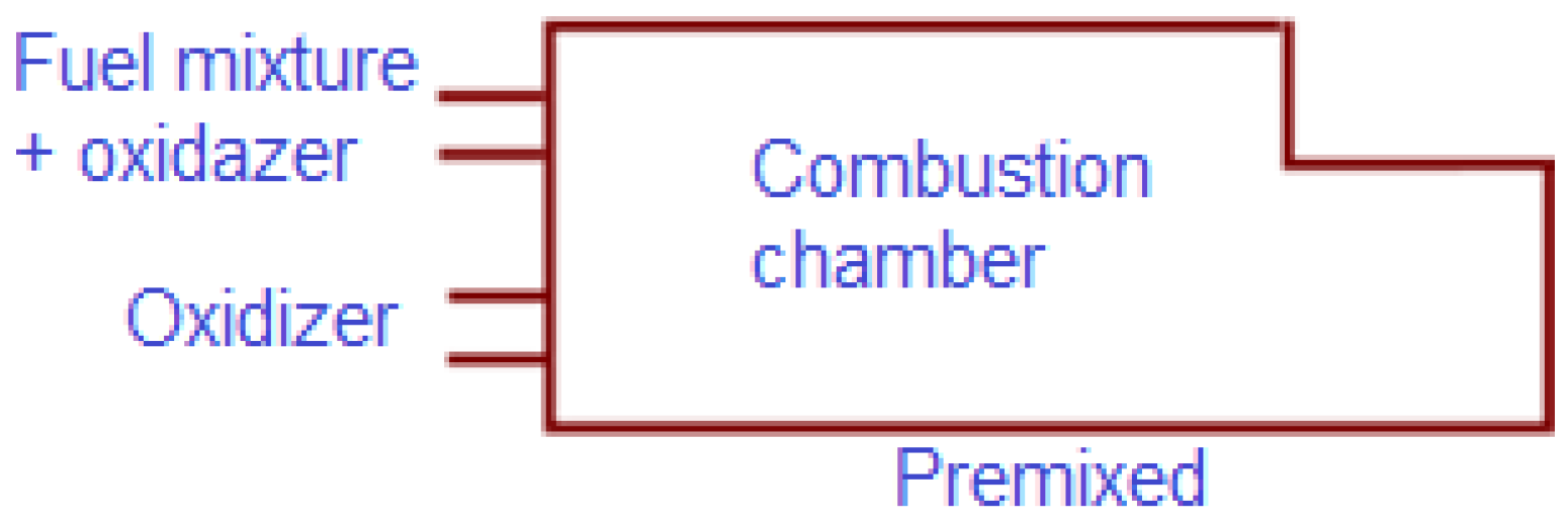
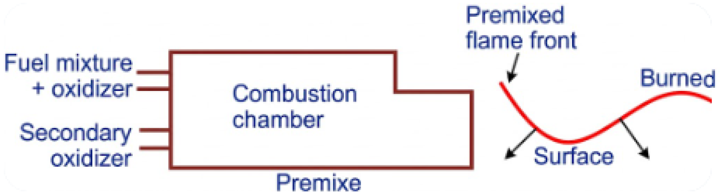
The furnace uses a residual fuel blend (industrial/automotive oils with solvents) as an alternative to traditional fossil fuels. This mixture is fed into the furnace at the end, along with a secondary oxidizer (air composed of N₂/O₂/Ar/CO₂), which moves toward the loading tunnel, as shown in Figure 1.

Within the designated premixing chamber, turbulent mixing occurred at 10% intensity, with a mixing scale of 1.5 mm.

2.2. Computational Domain: From Physical Geometry to Numerical Mesh

2.2.1. CAD Modeling

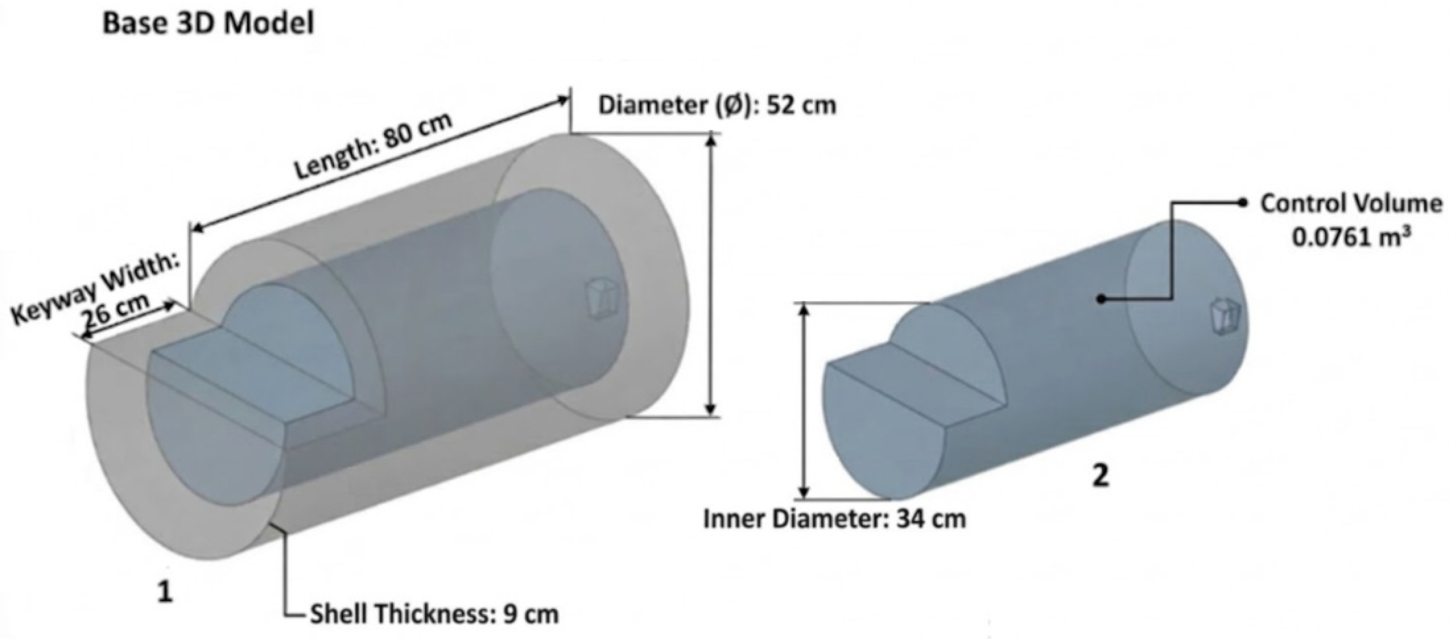
The initial phase involved creating a geometric model of the study system using computer-aided design (CAD). SolidWorks 2022 software (Dassault Systèmes) was employed for this purpose, chosen for its accuracy in modeling complex industrial geometries. The geometry was developed precisely in accordance with the technical specifications documented in Table 1.

This CAD model (visualized in Figure 2) served as the basis for subsequent simulations, ensuring that the numerical analyses accurately reflected the actual operating conditions of the IDR furnace, including detailed boundary conditions.

Dimensional accuracy was confirmed by comparing the model measurements with manufacturing drawings and on-site measurements of the physical equipment. This precise digital reconstruction allowed for the isolation of geometric variables in the combustion study, enabling direct data transfer to CFD simulation environments and establishing boundary conditions consistent with the furnace’s thermomechanical behavior.

2.2.2. CFD Software and Simulation Setup

The computational fluid dynamics simulation was conducted using ANSYS Fluent 2021 R2, a specialized thermofluidic modeling tool licensed for academic purposes [29]. The process started with importing the CAD geometry of the adjustable direct injection (ADI) oscillating furnace, with initial and boundary conditions based on real operating data.

These configurations allowed the simulation of important injection phenomena in the residual mixture and the analysis of temperature distributions and peak ranges. Additionally, the model captured crossflow effects on momentum transfer, turbulence generation, and volumetric heat release.

2.2.3. Mesh Generation

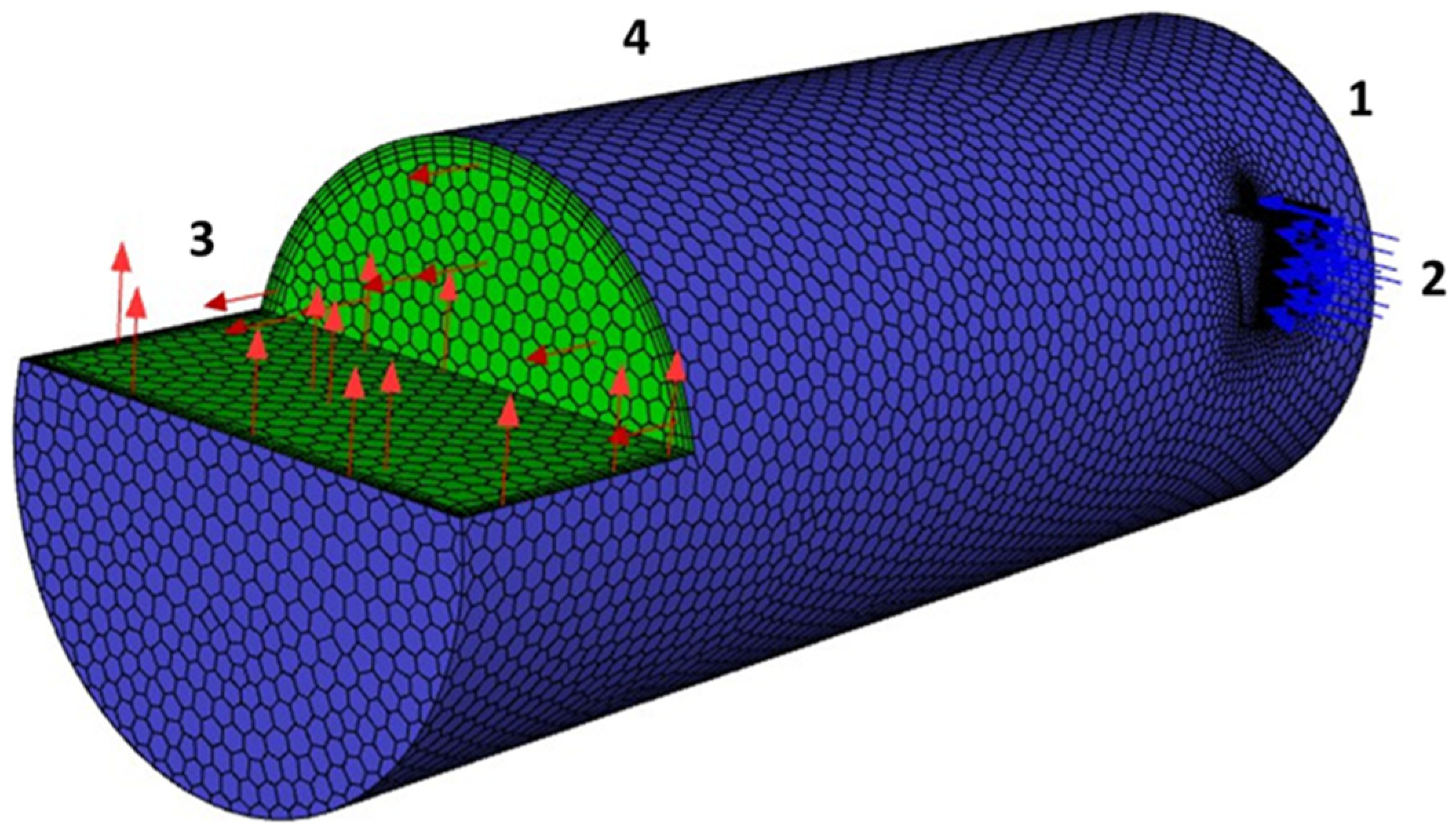
Figure 3 shows the axisymmetric combustion chamber model, in which a hybrid meshing strategy was used for domain discretization, with hexahedral cells near the nozzle and polyhedral cells elsewhere, along with refinements ranging from approximately 1.05 × 10⁵ to 1.10 × 10⁵ cells; the finest grid in the mesh-independence study included 109,600 cells. The mesh had an average element volume of 0.0761 mm³, as determined by a mesh independence study that confirmed errors of less than 2% in key parameters. This mesh includes injection parameters (primary/secondary flow), particle residence times, flow-stabilization patterns, and multilayer walls (refractory, insulating, external) with no-slip conditions. Fifteen inflation layers, starting with an initial thickness of 0.17 mm and a growth ratio of 1.2 (resulting in a total thickness of 36 mm), were used to maintain y⁺ < 1 under expected flow conditions. This boundary-layer mesh configuration accurately resolves the viscous sublayer, captures thermal gradients at the walls, and enhances numerical stability by extending to about 95% of the estimated hydrodynamic boundary-layer thickness (δ_h ≈ 32 mm).

2.2.4. Mesh Independence Study

The mesh independence study was conducted under full-load combustion conditions (open system, constant pressure), with incremental velocity and temperature profiles.

Table 2. Mesh analysis comparison.

No. of Cells	Max. Temperature °C	Max. Speed m·s−1
105,000	681	3.46
105,800	684	3.48
106,060	686	3.49
107,200	687	3.50
108,400	688	3.50
109,600	690	3.51

summarizes the validation and comparison of mesh analyses.

Simulations with coarser meshes exhibited bias due to poor resolution of flow features, whereas finer meshes did not significantly improve accuracy and only increased computational costs. The mesh containing 106,060 cells exhibited discrepancies below 2% when compared with the finest grid (109,600 cells) for both the peak temperature and maximum velocity, yielding deviations of 0.58% and 0.57%, respectively. Given the marginal improvement obtained with further refinement and the significantly higher computational cost, this mesh was selected as the optimal configuration for all subsequent simulations.

Integrated Mesh-Independence on QoIs: In addition to peak temperature and velocity, mesh-independence was evaluated for furnace-relevant integral quantities, including wall heat flux distributions, apparent heat-release rate, outlet/flue-gas temperature, and cycle-averaged thermal efficiency. Acceptance criteria were set to a variation of less than 5% between successive mesh refinements for each QoI within the stabilized operating window.

The solver used the finite volume method (FVM), implemented in C++, and employed in situ adaptive tabulation (ISAT) for modeling stiff chemistry.

This methodology proved robust and efficient, providing a reliable foundation for analyzing energy and environmental parameters in the IDR furnace while reducing computational costs through axial symmetry and mesh optimization.

2.3. Numerical Models and Governing Equations

2.3.1. Initial Conditions

At the start of the simulation, the furnace domain was initialized in a uniform, still state. The velocity field was set to 0 m·s⁻¹, and the pressure field to 0 Pa (gauge), providing a neutral baseline for the momentum equations. The temperature was set to 298.15 K (25 °C) uniformly, consistent with ambient conditions before operation. The initial gas composition consisted solely of the oxidizing mixture at rest, with mass fractions of 0.2100 for O₂ and 0.7900 for N₂, with no fuel vapors or combustion products present.

The turbulence model was initialized with neutral values—k = 1 × 10⁻⁶ m²/s² and ω = 1 s⁻¹—allowing the flow to develop naturally once the boundary conditions were applied. Radiation intensities in the Discrete Ordinates model were set to zero, reflecting the absence of thermal emission before ignition. No droplets were present initially; the liquid phase appears only after the injection boundary becomes active. These initial fields provide a consistent, physically grounded starting point for solving the reacting-flow equations in the IDR furnace.

2.3.2. Boundary Conditions

For physical accuracy, the simulation was set up to mimic realistic ventilation conditions, with secondary air entering at (10 m·s⁻¹, 26.85 °C) and primary air entering at (3.82 m·s⁻¹, 199.85 °C).

The species transport model examined combustion chemistry, beginning with the Air Injection Device (ADI) valve in the closed position, with nozzle conditions set to 4 bar and 90 °C. The oxidizer stream consisted of air with mass fractions of O₂: 0.2100 and N₂: 0.7900, while the fuel stream contained CO₂: 0.0721 and H₂O: 0.0279 by mass.

Time advancement utilized steady-state iterations (16,000) with pseudo-transient under-relaxation (effective pseudo-time step Δt = 1.0 × 10⁻³ s). A sensitivity analysis with a twofold increase or decrease in Δt showed that QoIs changed by less than 2%; time-step independence is addressed in Section 2.2.4 (QoIs variation < 5%).

2.3.3. Governing Equations

Continuity:

$$\partial \rho /\partial t+\nabla ·(\rho ·v⃗)=0$$

(1)

Momentum (RANS):

$$\partial (\rho ·v⃗)/\partial t+\nabla ·(\rho ·v⃗v⃗)=-\nabla p+\nabla ·\left[\right(\mu +\mu \_t\left)\right(\nabla v⃗+{(\nabla v⃗)}^{\mathrm{T}}\left)\right]+\rho ·g⃗+S\_m$$

(2)

Energy:

$$\partial \left(\rho h\right)/\partial t+\nabla ·(\rho ·v⃗·h)=\nabla ·\left[\right(k+k\_t/Pr\_t)\nabla \mathrm{T}]+S\_chem+S\_rad$$

(3)

Species:

$$\partial (\rho ·Y\_i)/\partial t+\nabla ·(\rho ·v⃗·Y\_i)=-\nabla ·J⃗\_i+\omega \_i$$

(4)

For clarity, detailed formulations are provided in Appendix A.

2.3.4. Physical Sub-Models

The simulation used advanced models: the k-ω SST model for turbulence; the Eddy Dissipation Concept (EDC) for combustion–turbulence interaction, applied uniformly across all simulations; and the Discrete Ordinates (DO) model for radiation, including participating gases (CO₂–H₂O).

Combustion closure (integrated): The furnace operates with a spray-dominated, partially premixed turbulent combustion regime. To ensure consistency in closure, the Eddy Dissipation Concept (EDC) was adopted as the single turbulent combustion model across all simulations. The previous references to premixed enthalpy transport and the G equation are replaced by this choice and are retained only for contextualization in the supplementary information. The EDC closure was selected because it couples turbulence time scales with finite-rate chemistry while remaining computationally feasible for industrial furnaces under spray evaporation and partial premixing.

Only the Eddy Dissipation Concept (EDC) model was used in all simulations and in the results reported in this study. References to premixed formulations or alternative closures are included solely to provide theoretical context and are not part of the computational approach employed.

For completeness, an alternative level-set G-equation formulation is summarized in Appendix A (Equation (A3)). All simulations here use the EDC closure.

2.3.5. Thermophysical Properties

The thermophysical properties of the gas mixture were treated as temperature-dependent and were obtained from the transport models available in ANSYS Fluent. For each species involved in combustion (O₂, N₂, CO₂, and H₂O), thermal conductivity was evaluated using the polynomial correlations provided in the solver’s transport library, and the mixture value was calculated through the standard mass fraction mixing rule. This ensures that conductivity develops consistently with both temperature and gas composition during the reaction.

Although the liquid thermal conductivity was not directly needed in the combustion model, the vapor-phase conductivity resulting from multicomponent evaporation was calculated internally by the solver using its species-based transport correlations.

2.4. Fuel Characterization and Injection Modeling

2.4.1. Fuel Composition and Properties

The injected residual mixture, composed of 94% C₂₀H₄₀, 4.5% C₈H₁₈, and 1.5% co-solvents, was thoroughly analyzed and confirmed to be free of solid particulates. Its specific properties are listed in

Table 3. Specification of a characterized mixture of residual oil and its solvent aggregates.

Characteristic Parameters	Unit	Sample
Viscosity at 20 °C	SSU (Saybolt Seconds Universal)	13.04
Gravity at 20 °C	°API	2.5
Specific gravity at 20 °C		0.9374
Water	%vol.	0.2
Insoluble in benzene	%wt.	≥0.2
Soluble in gasoline	%vol.	3–5

.

Fuel properties were determined experimentally. The density, viscosity, and flash point of the residual oil–solvent blend were measured following the corresponding ASTM standards: ASTM D1298 for density [46], ASTM D445 for viscosity [47], and ASTM D93 for flash point [48].

Table 4. Percentage mass content of the mixture.

Component	% Mass C	% Mass H	% Mass O	Proportion
C20H40	85.6281	14.3719		0.940
C8H18	84.1170	15.8830		0.045
C3H6O	62.0394	10.4128	27.5476	0.015
C8H10	90.5059	9.4941
C6H5CH3	91.2485	8.7515
C3H8	81.7136	18.2864
C4H8O	66.6283	11.1829	22.1888
C6H14O2	60.98	11.9410	27.0777

provides the detailed mass percentage composition of the mixture components.

2.4.2. Combustion Chemistry

The thermodynamic model incorporated conservation of atomic species (C, H, O, N) derived from the general combustion equation, thus ensuring an accurate representation of the chemical processes.

Upon ignition, the combustion process initiates an oxidation reaction, as shown in Equation (5), which represents the fundamental chemical change between the hydrocarbon fuel and the oxidizer.

$${\displaystyle \frac{1}{m_c}}{C}_a{H}_b{O}_c+\left(O_2+3.7N_2\right)⇾x_1{CO}_2+x_2{H}_{2}O+x_3{C}_a{H}_b{CO}_{2}H+x_4{H}_{2}O$$

(5)

where

$m_c$ = molar mass of the fuel;

$x_i$ = stoichiometric coefficients determined by atomic balance;

$C_a{H}_b{O}_c$ = partially oxidized hydrocarbon residue;

$C_a{H}_b{CO}_{2}H$ = carboxylic acid species formed during incomplete combustion.

This framework efficiently integrated flame geometry, turbulence, and chemistry, enabling the simulation of flame-front dynamics and emissions in turbulent fields within the chamber and providing kinematic tracking via the transport equation.

2.4.3. Chemical Mechanism Reduction

To reduce computational cost, a chemical mechanism reduction strategy was applied by decreasing the number of species (Nspecies) and reactions (Nreactions), with the reduction controlled by the empirical relationship in Equation (A4) (see Appendix B).

In this relationship, $C_1,C_2,C_3$ are thermochemical complexity constants, and $C_4\propto N\_species$ reflects the dependence observed in finite-difference reference systems. This simplification significantly accelerated the simulation without compromising physicochemical accuracy. As evidenced in Figure 4, during the complete combustion phase (burned gases), $N_{species}$ decreases drastically as complex reactants are transformed into stable products (CO₂, H₂O, N₂), thereby reducing the system’s dimensionality throughout the entire process, from injection to emission.

2.4.4. Spray Characterization and Multicomponent Particle Modeling

Spray parameters (final, reproducibility): The spray characterization, integrated with fuel injection, included nozzle type, flow rate, injection pressure, Sauter mean diameter (SMD), size distribution, spray cone angle, initial droplet temperature distribution, and models for breakup, collision, and coalescence (KH-RT or TAB). The final spray parameters for reproducibility were: SMD = 75 μm; size distribution: Rosin–Rammler (d_mean = 75 μm, q = 3.0); cone angle = 45°; breakup model = KH–RT; initial droplet temperature = 90 °C. Multicomponent evaporation follows Raoult’s law-based formulation with species-specific properties. Volatility characterization and a surrogate blending strategy for heavy waste oil components are detailed in Supplementary Table S1 (vapor-pressure curves and Antoine coefficients). The particle trajectory model uses a Lagrangian framework, integrating force balance over the multicomponent droplets of the residual mixture. The mass of each particle is calculated as the sum of its components’ masses, detailed in Table 4 by their proportion and percentage concentration (94% and 1.5% co-solvents).

This multicomponent model was operated by the furnace’s diffuse-injection Air Injection Device (ADI) system, which manages spatial dispersion based on experimentally validated pressure and turbulence profiles, as shown and discussed in Figure 1.

The vaporization rates of the components were determined using Equation (6):

$${\displaystyle \frac{{dm}_p}{dt}}=-\pi dp{\displaystyle \frac{\lambda g}{C_{p,g}}}Sh\times ln(1+Bm)$$

(6)

where B_m is the mass Spalding number, related to the concentration gradients derived from the species transport Equation (4).

The fractional vaporization rate was determined using Raoult’s Law, assuming the liquid phase to be a nearly ideal mixture of similar chemical species. In this case, non-volatile components are assumed to dissolve in volatile solvents, allowing for the exchange of mass, momentum, and energy.

Multicomponent particles were grouped into a finite number of packets with identical properties (position, velocity, temperature, size, density) and tracked from heating to vaporization using the energy equation (adapted from Equation (8)). This formulation employed discrete-phase modeling (DPM) and applied rate equations derived from a general energy balance.

Since the system is non-adiabatic, CFD simulation enabled characterization of latent heat during droplet formation at atmospheric pressure (1 atm) and modeled the thermal evolution of particles according to Equation (7) (see Appendix A, Equation (A4))

$$h_{fg}=-\underset{Tp}{\overset{T_{bp}}{\int }}{C}_{p,g}dT+h_{fg,bp}+\underset{T_p}{\overset{T_{bp}}{\int }}{C}_{p,p}dT$$

(7)

where $h_{fg}$ is the latent heat, $T_p$ the particle temperature, T_bp, the boiling point, $C_{p,g}$ and $C_{p,p}$ the specific heats of the gas and particle, respectively, and $h_{fg,bp}$ the enthalpy of vaporization at $T_{bp}$. Equation (8) describes the sensible enthalpy transfer (h) for fully premixed combustion:

$${\displaystyle \frac{\partial }{\partial t}}\left(\rho h\right)+▽·\left(\rho \overrightarrow{v}h\right)=▽·\left({\displaystyle \frac{k+k_t}{C_p}}▽h\right)+S_{h,chem}+S_{h,rad}$$

(8)

With $S_{h,chem}=\rho S_C{H}_{comb}{Y}_{fuel}$ (chemical source of enthalpy), where $S_C$ is the fuel consumption rate, $H_{comb}$ the calorific value, and $Y_{fuel}$ the fuel mass fraction.

As noted previously, the volatility characterization and surrogate blending strategy for heavy waste oil components are documented in Supplementary Table S1 (vapor-pressure curves and Antoine coefficients).

2.4.5. Note on Soot Modeling

It should be noted that although the CFD software used, ANSYS Fluent 2021 R2, predicts soot concentrations using empirical relationships, the available models are not compatible with the premixed combustion systems in this study, thereby limiting their use. This is further discussed in Section 2.6.3.

2.5. Experimental Validation Setup

2.5.1. Experimental Apparatus

For experimental validation, the IDR oscillating furnace was used with parameters matched to the simulation: velocity and pressure contours, a PAT (Process Analytical Technology) cycle with eight activities and 43 standardized tasks, two thermographic readers, and a 5-axis thermal imaging scanner. Reader 1 used laser-assisted spatial resolution (emissivity: 0.85–0.95); Reader 2 employed multifocal focus (thermal range: 200–1480 °C, accuracy ±0.5%), contrasting fuels: residual mixture versus traditional fossil fuels (diesel/gas). Comparative analysis of numerical and experimental data yielded the following: quantitative contrasts showed deviations of less than 5% in thermal profiles; characteristic inferences indicated improved efficiency in the residual mixture (84.6% vs. 46.2% in diesel); and key interactions revealed a correlation between turbulence (intensity of 10%) and flame stabilization.

PAT Framework Summary (added for clarity): eight activities include (i) ignition & warm-up, (ii) primary air/fuel stabilization, (iii) circumferential mixing ramp, (iv) load heating, (v) steady soak, (vi) controlled cooling, (vii) purge/vent, and (viii) idle/ready. The 43 standardized tasks represent the instrumented checkpoints and actuator operations within these activities (valving, flow/pressure checks, thermography scans, safety interlocks). A summarized list is available in Supplementary Table S2; site-specific details can be provided upon request.

2.5.2. Temperature Measurement

Temperature measurements were taken using two complementary infrared thermographic systems: a laser-assisted spatial thermographic reader with adjustable emissivity in the range of 0.85–0.95 and a multifocal thermal imaging scanner operating between 200 and 1480 °C, with an accuracy of ±0.5%. These instruments together enabled detailed characterization of internal chamber temperatures and external heat dissipation patterns.

2.5.3. Fuel Mass Flow Monitoring

Fuel mass flow rate was monitored using calibrated injection control equipment connected to the adjustable direct injection unit, while fuel properties (including its LHV) were determined from previous physicochemical analysis of the residual oil–solvent blend.

2.5.4. Comparative Testing Protocol

Comparative tests using diesel and natural gas were conducted in the same IDR furnace and under identical operating conditions as those for the residual oil–solvent blend. The purpose of these tests was not to separately optimize each fuel but to compare their performance under equivalent process conditions.

For all fuels, the furnace geometry, injection equipment, PAT control logic, load conditions, ventilation setup, and boundary conditions remained unchanged. Fuel switching was performed while maintaining the same thermal demand, process cycle, and operational constraints, so that fuel type was the only intentional independent variable.

Because of differences in the physicochemical properties of fuels and in injection systems, identical numerical equivalence ratios were not applied across fuels. Instead, equivalence was achieved at the process level by ensuring comparable thermal output and stable combustion conditions, confirmed through temperature profiles, pressure stability, flame behavior, and cycle repeatability.

The secondary airflow rate, ventilation setup, and residence-time limits were fixed by design and stayed the same across all comparative tests. Apparent combustion behavior was assessed using combined CFD predictions and thermographic measurements instead of directly measuring the laminar flame speed.

Repeatability was evaluated across complete operational cycles defined by the PAT framework. Performance metrics were averaged over stable operating periods for each fuel, and the sources of uncertainty affecting all fuels are similarly considered, ensuring the validity of relative comparisons within the estimated uncertainty ranges.

2.5.5. Validation Results

The comparative analysis of numerical and experimental data revealed the following: quantitative comparisons showed deviations less than 5% in the thermal profiles; characteristic insights indicated improved efficiency of the residual mixture (84.6% versus 46.2% in diesel); and key interactions demonstrated a correlation between turbulence intensity (10%) and flame stabilization.

2.6. Exhaust Emissions Measurement and Computation

2.6.1. Experimental Emissions Measurement

Exhaust emissions were evaluated using a combined measurement and calculation approach. For CO and CO₂, non-dispersive infrared (NDIR) analyzers were employed with continuous sampling at the exhaust duct under steady operating conditions. Total unburned hydrocarbons (THC) were measured with a flame ionization detector (FID), while NOx levels were determined with a chemiluminescence analyzer. Sampling was carried out downstream of the mixing section to ensure that the flue gases were representative and well mixed. Calibration checks were performed before and after each measurement session.

2.6.2. Computational Emissions Estimation

Additionally, theoretical emission estimates were derived by post-processing CFD fields. Thermal NOx was calculated from the simulated temperature and oxygen distributions using the extended Zeldovich mechanism, while prompt NOx (Fenimore) contributions were assessed using local equivalence ratio and high-temperature residence time as indicators. CO and THC trends were determined from the species transport solution and the extent of complete oxidation along the main reaction and post-flame zones.

2.6.3. Soot Modeling Scope and Radiative Transfer Treatment

Soot formation was not explicitly modeled in the CFD. The combustion setup employed a premixed, turbulence-controlled regime, and the radiation field was calculated using the Discrete Ordinates (DO) model, considering gas-phase participating media (CO₂–H₂O). The soot submodels available in the chosen solver were incompatible with the fully premixed configuration, which limited their use in this case.

To reduce potential biases in radiative heat transfer caused by neglecting soot, two measures were taken: (i) experimental thermography was used to estimate wall heat fluxes and external radiative losses, and (ii) sensitivity analyses were conducted by bracketing the gas-only absorption with effective absorption coefficients representing low-soot and soot-free conditions.

2.7. Data Analysis and Performance Metrics

2.7.1. Relationships Between Study Variables

In the numerical simulation, 16,000 iterations were conducted, corresponding to a full IDR furnace cycle. To analyze the process behavior, key variables such as speed, energy constant, stability, and residual emissions were measured and synchronized. Their relative relationships and behaviors were assessed based on the accuracy of the simulated cycle. In this model, the velocity stabilizes in its three components (x, y, z), while the turbulent kinetic energy of the system (omega) remains constant. Once this stage is complete, the mixture in the combustion process releases water vapor, either present or generated by the released energy. This phenomenon helps determine the equilibrium constant (k) of the controlled chemical model, which is essential for maintaining the continuity and stability of the combustion process within the parameters defined for each work cycle.

2.7.2. Definition of Thermal Efficiency

The thermal efficiency of the adjustable direct injection reciprocating (IDR) furnace was defined on a lower heating value (LHV) basis as the ratio of useful heat transferred to the process to the chemical energy supplied by the fuel. The LHV was chosen over the higher heating value (HHV) to reflect realistic industrial operating conditions, in which the water vapor produced during combustion is not condensed, and its latent heat is not recovered.

Accordingly, the thermal efficiency (n_th) was calculated using Equation (9):

$$n_{th}(\%)={\displaystyle \frac{Q_{useful}}{{\mathrm{ṁ}}_{fuel}\cdot LHV}}·100$$

(9)

where Q_useful represents the net useful heat transferred to the furnace chamber and processed load, ṁ_fuel is the mass flow rate of the residual fuel blend, and LHV refers to the experimentally determined lower heating value of the fuel mixture. The useful heat is defined as the energy that contributes to the thermal rise and stabilization of the furnace chamber during steady operation, excluding heat losses through the exhaust gases, furnace walls, and external radiation.

2.7.3. Energy Balance and Heat Loss Estimation

A global energy balance was established to ensure consistency in thermal efficiency calculations and to identify the dominant heat-loss mechanisms in the IDR furnace. The chemical energy supplied by the fuel was partitioned into useful heat and several loss components according to Equation (10):

$${ṁ}_{\mathrm{fuel}}\cdot \mathrm{LHV}=Q_{\mathrm{useful}}+Q_{\mathrm{exhaust}}+Q_{\mathrm{walls}}+Q_{\mathrm{radiation}}+Q_{\mathrm{unaccounted}}$$

(10)

where $Q_{\mathrm{exhaust}}$ represents thermal losses associated with high-temperature combustion gases discharged through the exhaust duct, $Q_{\mathrm{walls}}$ accounts for conductive and convective losses through the refractory lining and external steel casing, and $Q_{\mathrm{radiation}}$ corresponds to radiative emission from the external furnace surfaces. Minor residual terms—including measurement dispersion, operational fluctuations, and small transient effects—were grouped under $Q_{\mathrm{unaccounted}}$, remaining below 5% of the total energy input.

To refine the estimation of these loss terms, heat fluxes through the walls and exhaust stream were quantified by coupling CFD-predicted temperature and velocity fields with experimental thermographic measurements. This combined numerical–experimental strategy enabled spatially resolved identification of heat-loss regions, reducing reliance on lumped or empirical correlations and improving the robustness of the furnace energy assessment.

2.7.4. Uncertainty Assessment

Considering the combined uncertainties associated with flow-rate measurement, LHV determination, thermographic readings, and CFD-based heat-flux estimation, the overall uncertainty in the calculated thermal efficiency remained within ±6%, a value consistent with industrial furnace efficiency assessments.

2.7.5. Operating Cost Accounting Framework

Alongside the thermal balance, an operating cost accounting framework was incorporated to link energy performance to economic impact. The assessment includes factors such as fuel price, specific fuel consumption per cycle (L/cycle), energy cost per unit of useful heat (MXN per MJ_LHV), and maintenance and cleaning requirements associated with furnace operation. Throughput (mass or number of parts processed per hour) and cycle-time reductions were analyzed under consistent thermal-demand conditions across all fuels. Uncertainty ranges were used to standardize these metrics across different operating states, ensuring comparability. Supplementary Table S2 outlines the data structure collected per run, which includes fuel use logs, thermal input/output measurements, and operational cost records.

2.8. Summary of Methodological Framework

Overall, the combined energy balance and operating cost analysis creates a unified framework for measuring the thermoeconomic performance of the furnace, allowing the identification of main heat loss pathways and the economic impacts of alternative fuels.

This methodology proved robust and efficient, providing a reliable basis for analyzing energy and environmental parameters in the IDR furnace while reducing computational costs through axial symmetry and mesh optimization.

3. Results

3.1. Thermal, Velocity, and Pressure Fields Obtained from CFD Simulation

A comprehensive CFD campaign was carried out to analyze the thermo–fluid-dynamic behavior of the adjustable direct-injection reciprocating (IDR) furnace powered by a residual oil–solvent blend. The numerical results detail temperature distributions, velocity fields, and pressure gradients within the combustion chamber under typical operating conditions.

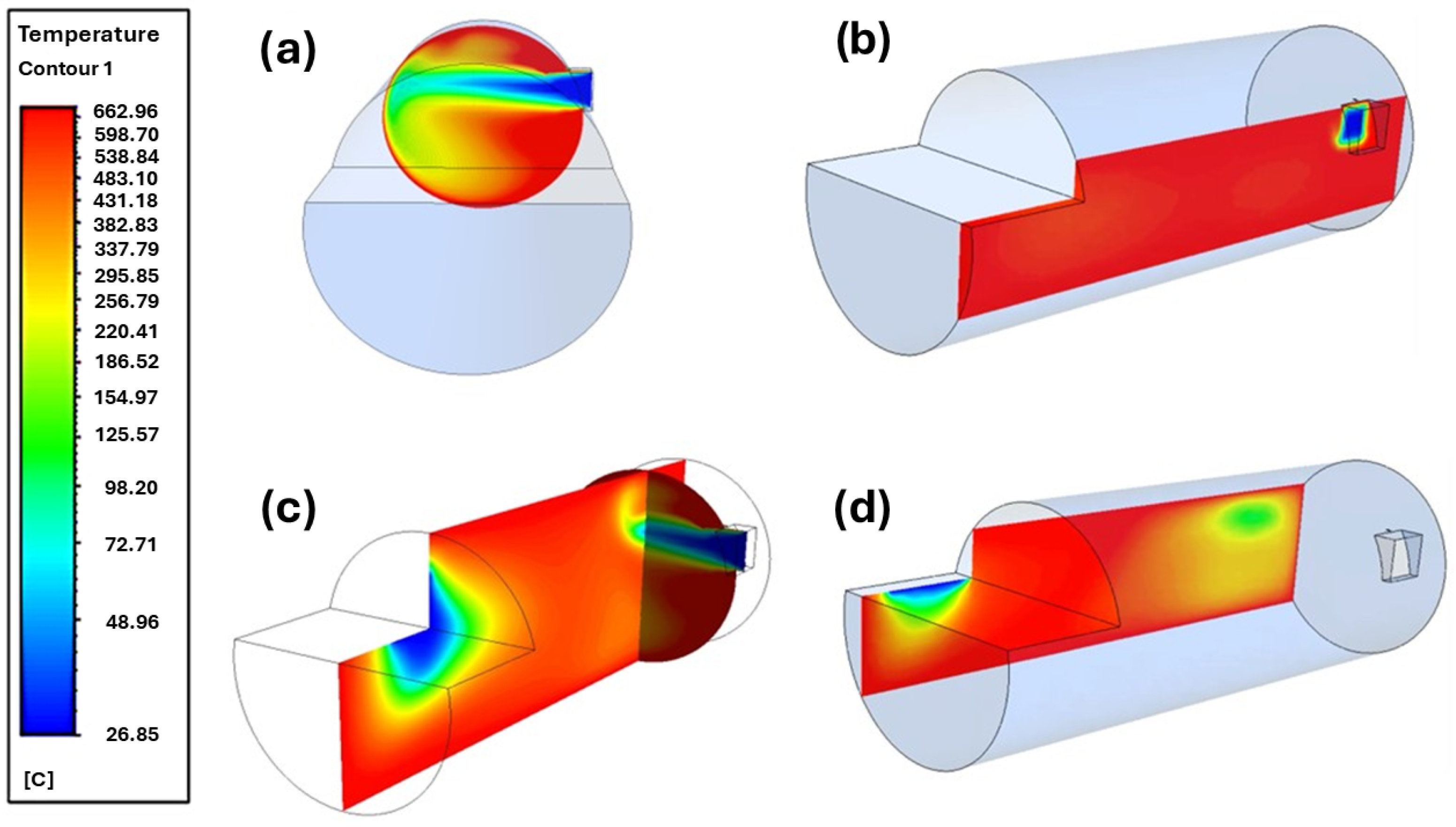
Figure 5 illustrates the temperature contours throughout the simulated combustion cycle. Four key stages can be identified. First, ignition begins near the injection zone at around 90 °C, with a laminar flame front driven by the interaction between the compressed oxidant stream (N₂/O₂/Ar/CO₂) and the injected mixture, resulting in a local wall temperature above 200 °C. Second, a change in trajectory causes double-displacement turbulence along the chamber’s circumference, which enhances heat diffusion and spreads the thermal field toward the open exhaust zone; temperatures become uniform across the chamber at about 568.7 °C. Third, perpendicular sections reveal zones of thermal generation, propagation, residence, and exit, aligning with the synchronization of furnace operation with 43 PAT tasks. Finally, the temperature spread (90–662.96 °C) matches multifocal thermography, confirming the model’s enforced axial symmetry.

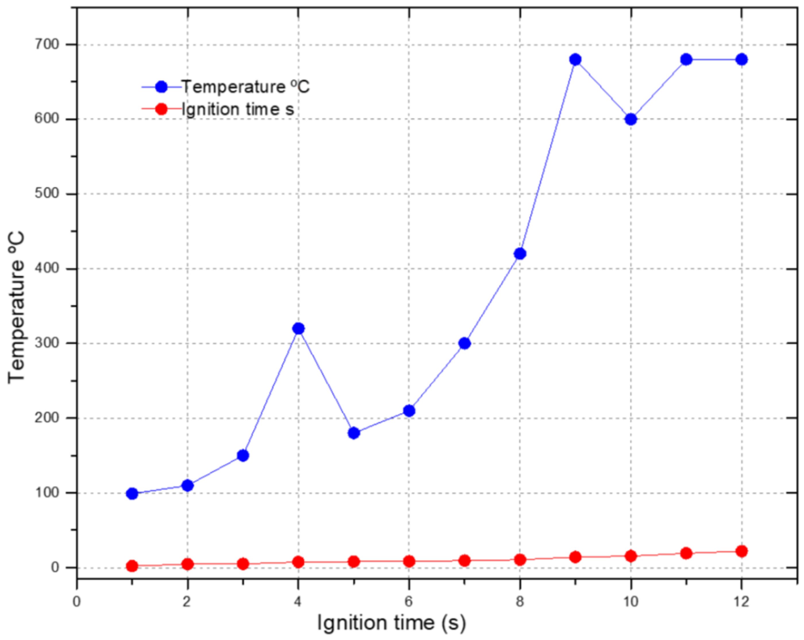
Figure 6 depicts the temporal evolution of the thermal field. Geometry-induced turbulence enables rapid ignition at low initial temperatures, and as gas residence time increases, the temperature rises until it stabilizes at approximately 700 °C. This evolution matches the three PAT phases: heating, propagation, and stabilization.

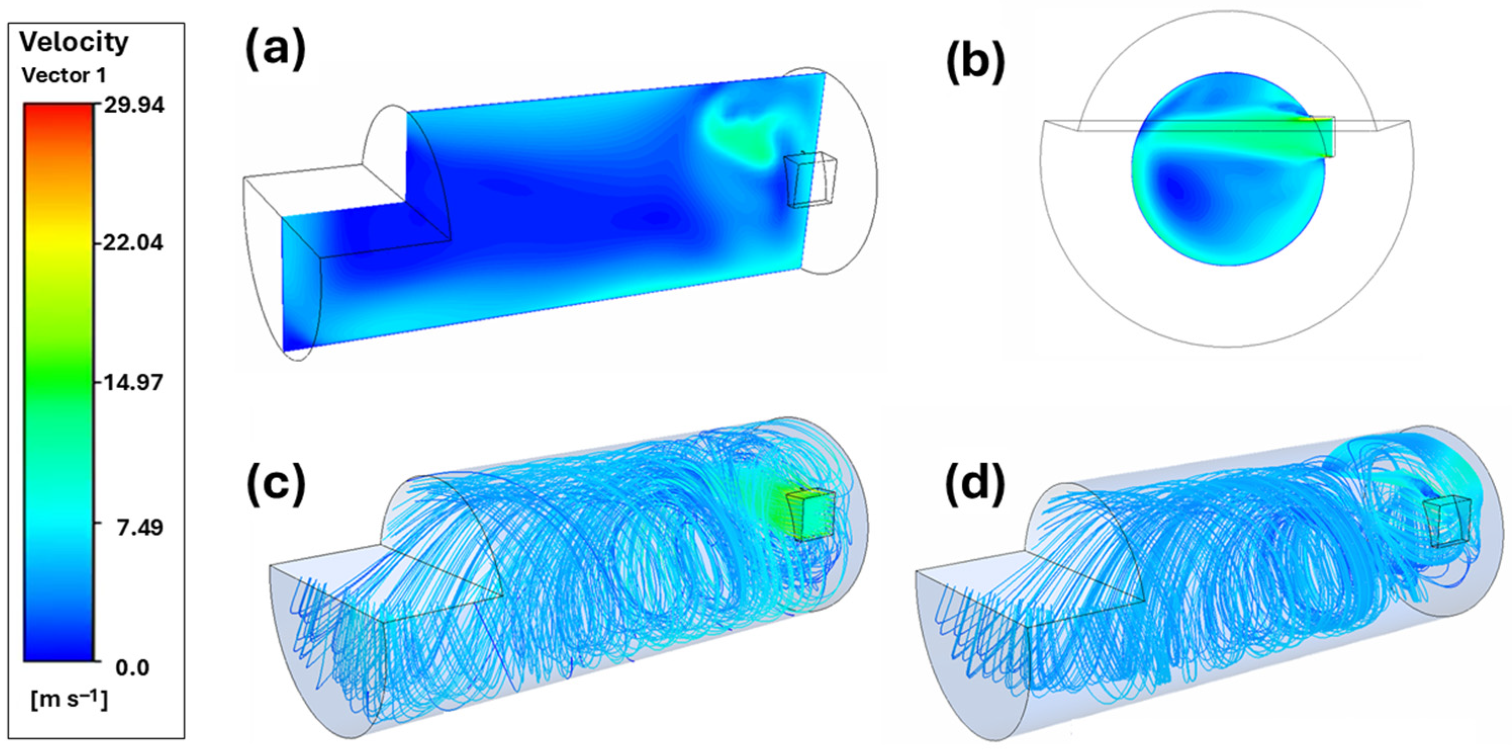
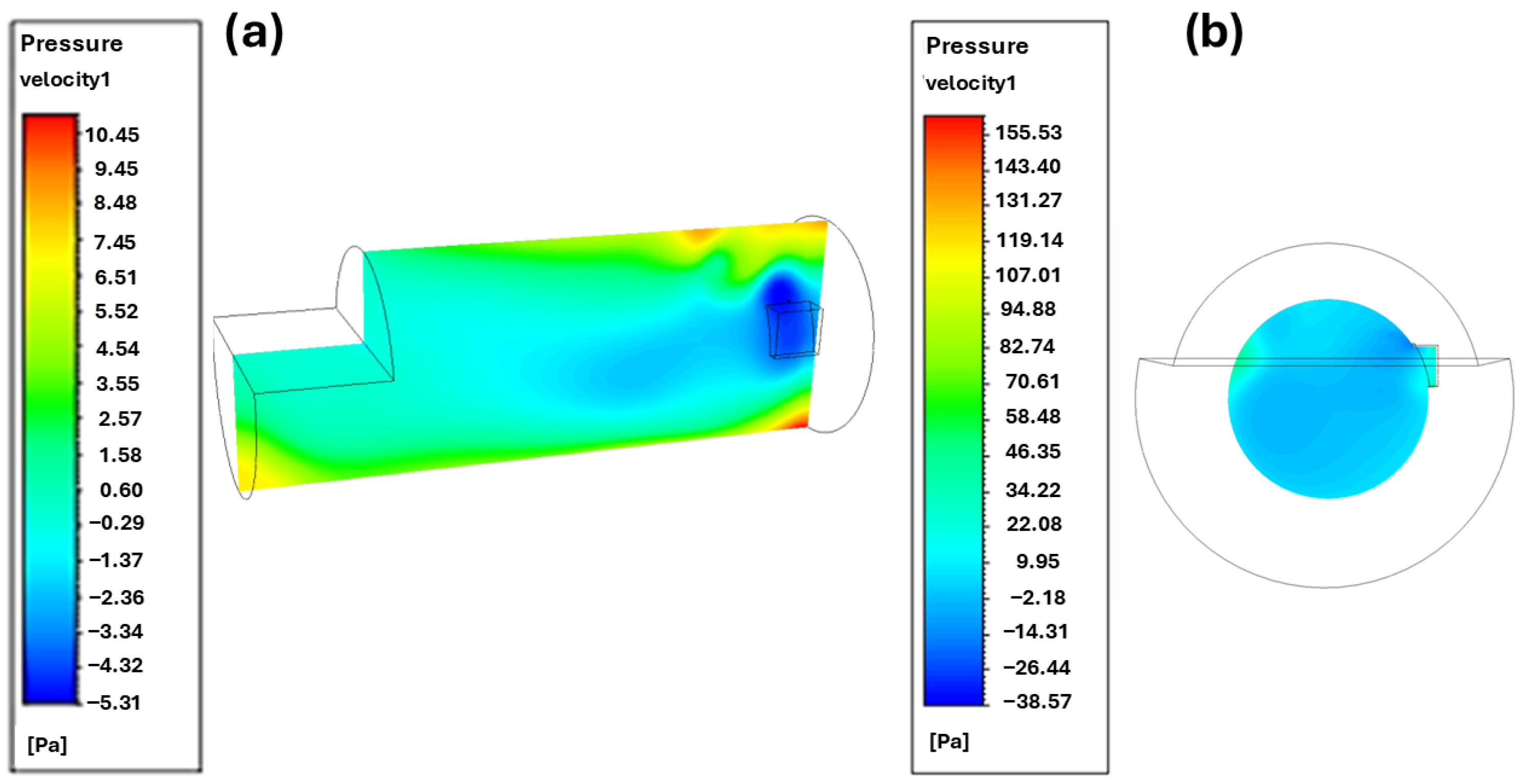
Velocity contours in Figure 7 illustrate the role of the oxidizer stream in guiding and stabilizing the flame. Turbulence forms near the injection area, shaping the initial flame path with a cyclic circumferential pattern. The flame hits stationary walls at about 7.5 m·s⁻¹, matching the secondary air boundary condition of 10 m·s⁻¹. As combustion continues, the flow around the circumference stabilizes at roughly 3.82 m·s⁻¹, indicating the interaction between the compressed oxidant and the fuel mixture. An extra injection alters the flow response, showing the model’s sensitivity to operational changes.

Pressure fields (Figure 8) indicate that negative pressures are avoided during ignition. As gases discharge above 600 °C, a chimney effect develops, while the highest pressures cluster around the ignition circumference prior to furnace movement. These pressure patterns regulate evacuation and limit uncontrolled heat losses, contributing to stable thermal performance.

3.2. Experimental Thermographic Results

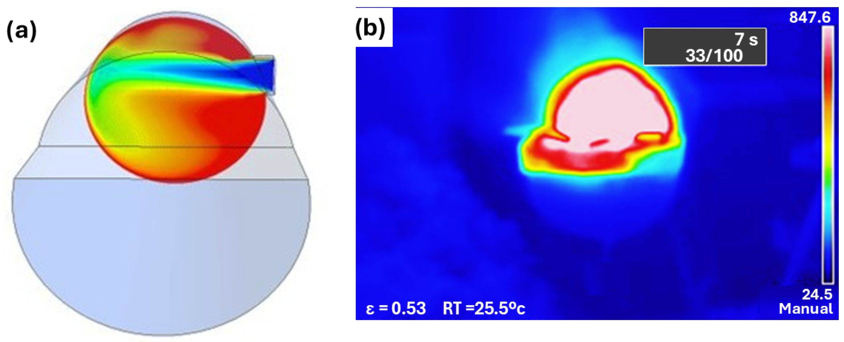
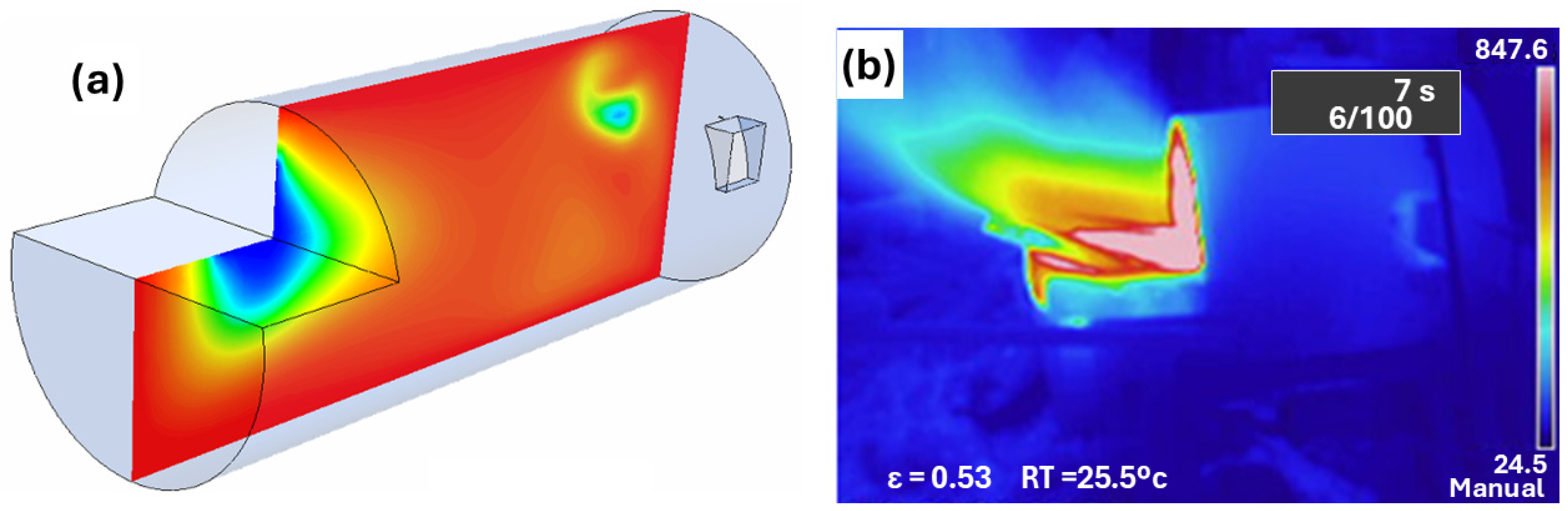
Infrared thermography was employed for experimental validation under conditions equivalent to those used in the numerical model, using two independent thermal imaging systems (spatial and multifocal configurations). Figure 9 and Figure 10 provide complementary thermographic perspectives that, when compared, reveal a coherent interpretation of the thermal behavior of the IDR furnace.

Figure 9 illustrates the contrast between numerical predictions and experimental measurements during the preheating phase, when localized thermal residues form due to cumulative heat storage. This moderated temperature distribution is consistent with the transient thermal buildup expected prior to achieving full operational stabilization.

Figure 10, in contrast, presents the internal temperature contours obtained from the CFD simulation alongside the externally measured thermal contours during stabilized operation. The internal simulation results confirm the presence of a high-temperature region near the exit zone under RDI/PAT-controlled conditions, whereas the external measurements reveal a gradual heat dissipation pattern characterized by minor transient fluctuations. Together, these two figures demonstrate a clear correspondence between the internal thermal stability predicted by the CFD model and the moderated external thermal behavior observed experimentally. This agreement supports the model’s capacity to accurately reproduce both transient and steady-state thermal responses of the IDR furnace.

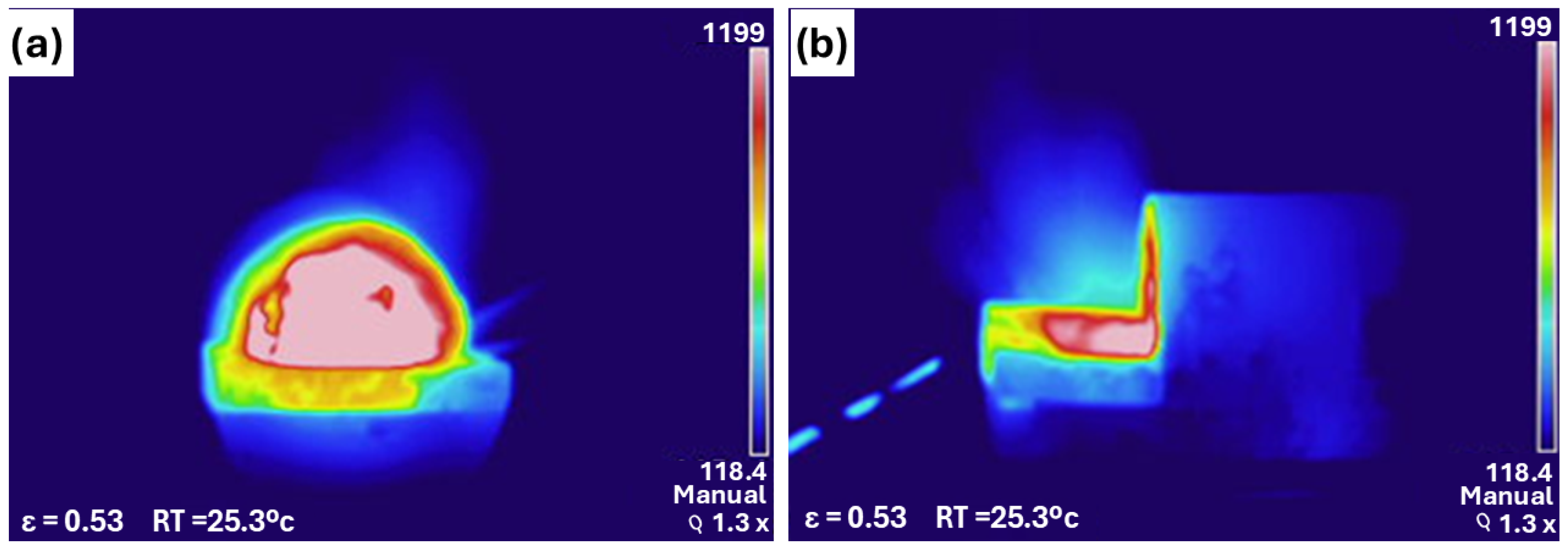
Prior to full process stabilization, higher internal readings were recorded: a maximum of 1199 °C inside the chamber (Figure 11a), accompanied by lower external outlet temperatures (Figure 11b), indicating effective internal heat retention and controlled dissipation.

A direct quantitative comparison between the simulated and experimentally measured temperature profiles at corresponding axial positions shows deviations of less than 5% (see

Table 5. Deviations between CFD predictions and thermographic measurements with uncertainty bounds.

Location	CFD Temperature (°C)	Thermographic Temperature (°C)	Deviation (%)
Injection region	568	590	3.8
Mid-chamber	616	643	4.2
Exit zone	639	670	4.6

). This agreement was verified by extracting temperature traces from both the CFD fields and the thermographic measurements during stabilized operation. For example, at the principal monitoring locations (injection region, mid-chamber, and exit zone), the maximum difference did not exceed 3.8%, 4.2%, and 4.6%, respectively. These values fall within the uncertainty bounds of the thermographic instruments and confirm the accuracy of the CFD model in reproducing the furnace’s thermal behavior.

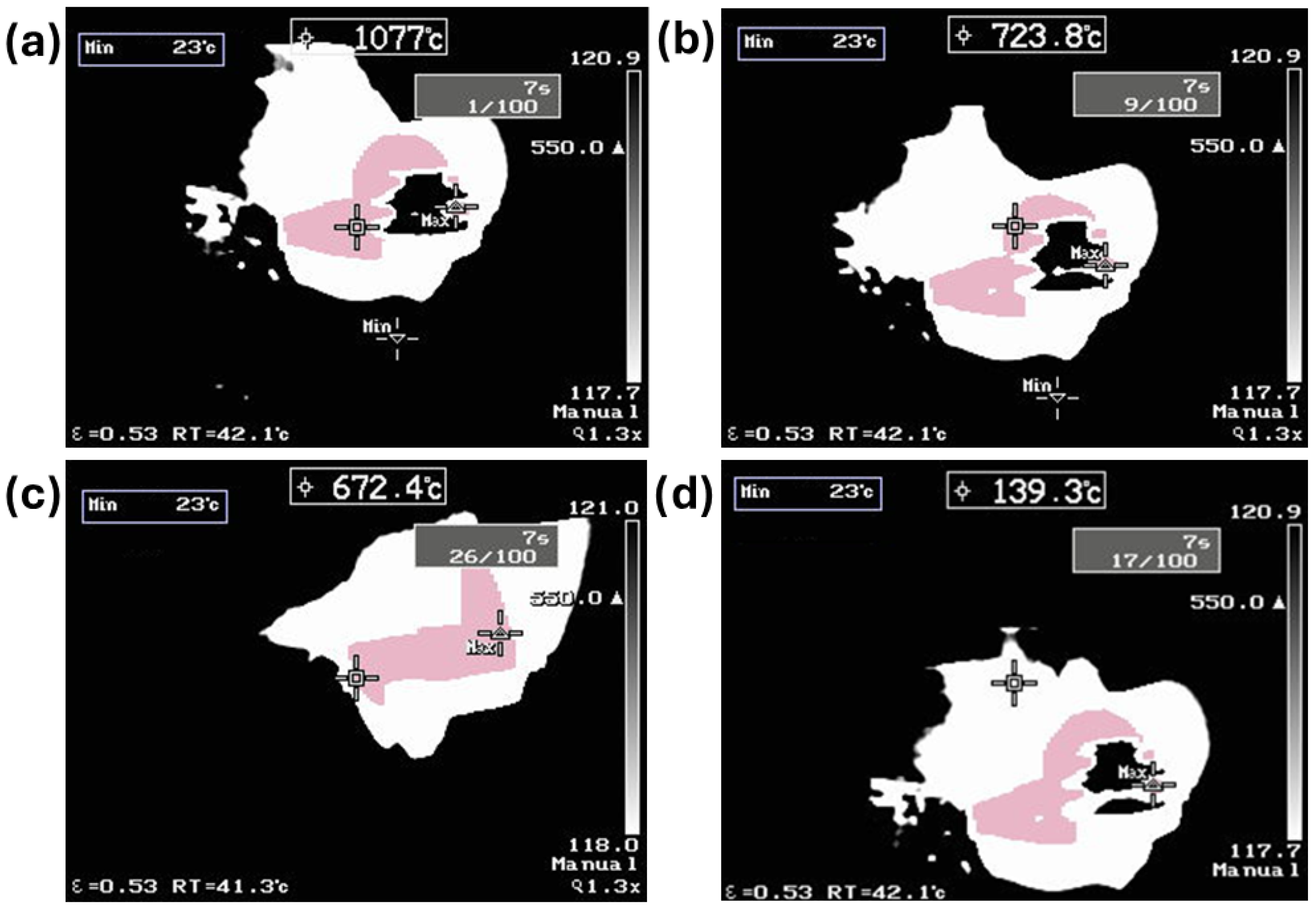
Consistency with Figure 12: The temporal thermal evolution shown in Figure 12 is fully consistent with the behavior reported in Figure 9, Figure 10 and Figure 11. The internal peak temperatures, subsequent stabilization, and gradual external cooldown, as captured in the spectral sequence of Figure 12, confirm the cyclical heating–stabilization–cooling pattern imposed by the PAT-controlled operation. This figure demonstrates that the internal temperature distribution predicted by the CFD model aligns with the experimentally observed stabilization phases, reinforcing the validity of the combined numerical–experimental approach.

All comparative performance metrics reported in this section (diesel, natural gas, and residual blend) were obtained under operating conditions equivalent to those described in Section 2.5.4. Accordingly, the observed differences reflect intrinsic fuel effects within the same industrial process rather than variations in furnace configuration, control strategy, or load conditions.

Exhaust emissions: theoretical estimates and experimental proxies.

Under stabilized operation, measured exhaust streams displayed CO and THC levels consistent with near-complete oxidation in the main reaction zone, while NOx tendencies correlated with local peak temperatures identified in the CFD fields. Theoretical post-processing indicated that thermal NOx formation is favored in regions approaching the maximum internal temperatures, whereas prompt NOx remains limited by the predominantly premixed regime and short high-temperature residence times near stoichiometric conditions.

The comparative interpretation presented in this section is grounded on the operating equivalence defined in Section 2.5.4. Consequently, differences discussed between diesel, natural gas, and the residual oil–solvent blend are attributed to intrinsic fuel properties and combustion behavior within the same industrial framework, rather than to variations in operating conditions, control strategy, or furnace configuration.

Soot was not directly quantified; however, the absence of radiative signatures indicative of heavy soot loading in the thermographic records, together with the premixed/turbulent mixing conditions, supports the expectation of low soot yields under the studied operating window. Nevertheless, localized transient richness near the injection zone cannot be entirely excluded and will be addressed in future targeted measurements.

3.3. CFD–Experimental Comparison and Model Validation

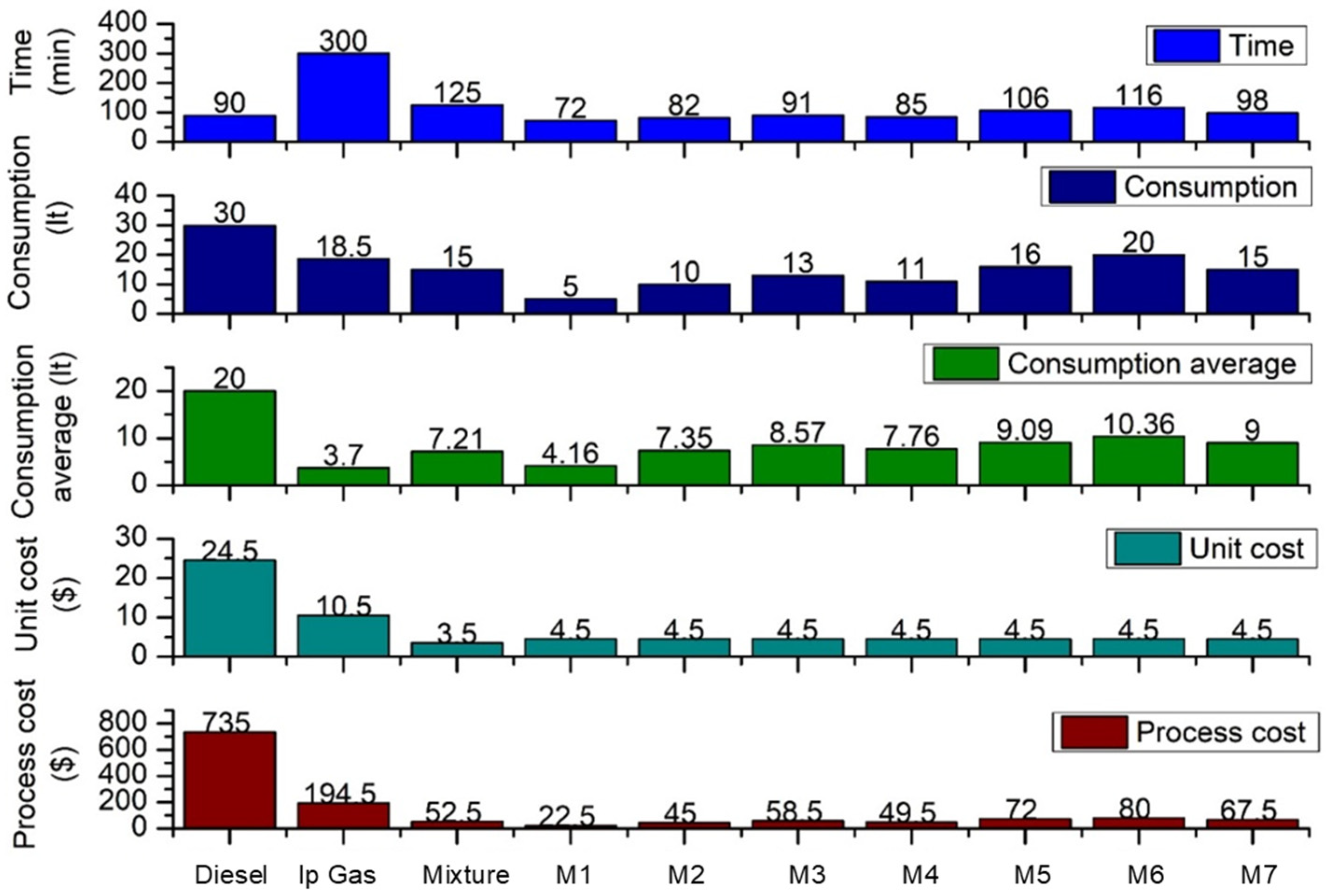
A direct comparison between CFD predictions and experimental thermographic measurements shows deviations of less than 5% across the temperature profiles, confirming that the numerical model reliably reproduces the dominant thermo–fluid–dynamic mechanisms governing combustion in the IDR furnace. As clarified for Figure 13, the fuel samples labeled M1–M7 correspond to distinct characterized blends; in this study, sample M1 is emphasized because it exhibits the most favorable properties listed in Table 3 and serves as the reference mixture for all comparative metrics. The absolute experimental values used for normalization—including cycle time, fuel consumption, and operating cost—are provided in Supplementary Table S3, which serves as the reference dataset for the calculations presented in this section. To enable direct comparison between fuels, performance indicators were normalized with respect to the baseline experimental reference according to

$$\eta ={\displaystyle \frac{X_{\mathrm{fuel}}-X_{\mathrm{ref}}}{X_{\mathrm{ref}}}}\times 100\%$$

(11)

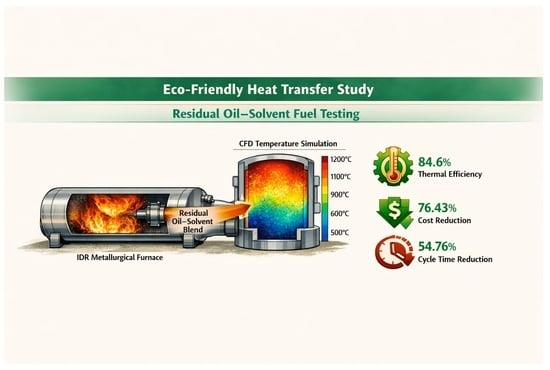
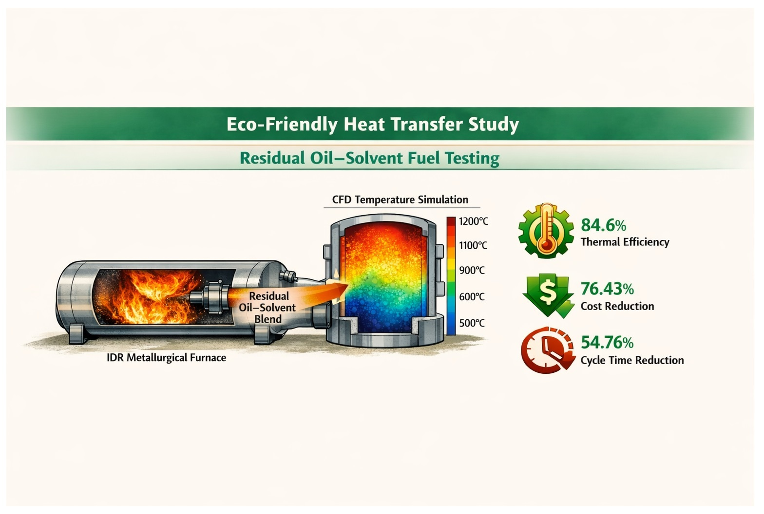
Using the experimental values reported in Supplementary Table S3 and the comparative trends shown in Figure 13, this normalization yields a 54.76% reduction in cycle time and a 76.43% reduction in operating cost for the M1 blend relative to conventional diesel. These values are fully consistent with the energy-balance and operating-cost analyses presented in Section 2.7.3 and Section 2.7.5, confirming the superior thermo-economic performance of M1 within the validated CFD–experimental framework.

Figure 13 consolidates key performance outcomes for the residual blend (M1) relative to conventional fuels (diesel and LP gas). The results consistently demonstrate M1’s superior thermal reach, faster stabilization behavior, and higher apparent heat release rate, reflecting the synergistic effects of multicomponent evaporation, turbulence-enhanced mixing, and radiative heat transfer. The model’s ability to reproduce these phenomena with high fidelity indicates that the CFD framework captures interactions among turbulence, mixing processes, radiative transport, and multicomponent droplet dynamics.

Overall, the close agreement between numerical predictions and experimental measurements validates the CFD model as a robust predictive and optimization tool for industrial furnace operation. Its demonstrated accuracy in representing combustion stability, heat transfer behavior, and energy-efficiency trends supports its applicability to process analysis, optimization, and fuel-substitution strategies in metallurgical systems.

4. Discussion

4.1. Influence of Turbulence and Flow Structure on Combustion Stability

Combustion stability in the IDR furnace is controlled by turbulence-driven regimes, characterized by Damköhler numbers below one. In these conditions, rapid premixing occurs, resulting in a thin reaction zone and spatially uniform equivalence ratios. The Damköhler number was estimated as the ratio of the characteristic turbulent mixing time to the chemical reaction time derived from the EDC fine-structure reaction rate. Under the furnace operating conditions, this ratio stayed below 1, confirming that combustion occurs in a turbulence-dominated regime.

This behavior aligns with previous research on turbulence–chemistry interaction in premixed and partly premixed flames [30,32]. The close match between CFD predictions and thermographic measurements (with deviations consistently below 5%) confirms that the model accurately captures the primary thermo-fluid mechanisms governing furnace operation.

Studies on industrial furnaces equipped with wall-mounted or staged burners also report improved stabilization and residence time control, driven by turbulence intensity and circumferential flow structures. Arrieta-Burgos et al. identified similar stabilization patterns in radiant burner configurations, while Jung et al. linked turbulent mixing directly to combustion completeness. The present work extends these observations by demonstrating that these mechanisms remain valid under more complex multicomponent fuel conditions, such as residual oil–solvent blends with adjustable direct injection, reinforcing the applicability of Da < 1 stabilization beyond conventional fuel systems [18].

4.2. Thermal Efficiency and Heat Retention Mechanisms

Thermal homogenization decreases wall-normal gradients and lessens convective and radiative losses, thereby improving internal heat retention. Stable pressure fields help contain heat and shorten stabilization time, aligning with the PAT-defined thermal stages observed experimentally.

Previous studies report improvements in thermal efficiency when optimizing air–fuel interaction in industrial heating furnaces operating with conventional fuels, although typical peak temperatures rarely exceed 800 °C. In contrast, the present work demonstrates that residual oil–solvent blends can sustain peak temperatures of up to 1199 °C while maintaining controlled external dissipation. This suggests that the combined effect of turbulence control, PAT-based operation, and multicomponent vaporization behavior enables superior efficiency compared with optimized fossil-fuel systems [33].

4.3. Emissions Performance and Soot–Radiation Coupling

The combined experimental–numerical framework offers a clear explanation of emissions trends. Although higher peak temperatures generally increase thermal NOx formation, the partially premixed regime and controlled fuel injection decrease unburned species and inhibit soot-forming zones, reflecting traditional thermal and mixing-controlled trade-offs [34,35].

Although explicit soot modeling was not included, uncertainties in radiative transfer are bounded using thermographic observations and energy-balance consistency checks. This suggests that soot–radiation effects do not significantly alter the reported efficiency trends. Future work should incorporate compatible soot models or hybrid correlations based on direct sampling to improve radiative-heat predictions under expanded operating conditions [36].

4.4. Influence of Residual Fuel Composition on Performance

Under similar operating conditions, the residual oil–solvent mixture exhibits stable combustion, greater thermal reach, and emission performance comparable to traditional fuels used in industrial furnaces. The improved behavior results from interactions between heavier hydrocarbons and light solvent fractions, which accelerate droplet heating, vaporization, and oxidation, thereby allowing higher maximum temperatures and greater apparent heat release. These effects stem from multicomponent chemical kinetics combined with turbulent mixing, rather than from any single component.

4.5. Modeling Limitations and Alternatives

The RANS–EDC model adequately represents global furnace behavior—such as efficiency, heat flux distribution, and outlet temperature—and remains computationally manageable for industrial applications. However, it cannot fully capture unsteady flame dynamics or the stratification characteristic of partially premixed turbulent regimes. LES-based closures, including Thickened Flame or flamelet/FGM tabulation, provide higher accuracy at increased computational cost. The chosen approach is justified by the focus on integral furnace metrics and the availability of experimental constraints; model-form uncertainty is acknowledged and bounded through validation and sensitivity analyses [37].

4.6. Environmental Performance and Operational Reliability

Environmental evaluation must consider emissions (O₂, CO, CO₂, NOx, THC), soot propensity, potential impacts on metals/ash, and operational reliability (fouling, maintenance intervals). The combination of CFD prediction, thermographic validation, and flue gas analysis across multiple cycles enables a transparent assessment of environmental and reliability indicators relevant to industrial applications.

Previous research has focused on single-component or slightly oxygenated fuels (such as biomass oils and gaseous alternatives), which exhibit different impacts on radiative transfer and stability. For example, Bäckström et al. highlighted composition-dependent radiative behavior in rotary kilns, and Yan et al. stressed the importance of fuel uniformity and injection stability in smelting furnaces. The current study extends this work by demonstrating that a controlled, multicomponent residual blend can provide greater thermal reach and quicker stabilization without sacrificing stability, as confirmed by CFD and thermographic validation.

4.7. Operational Implications and Process Optimization

Integrating CFD predictions, PAT-enabled control, and thermographic measurements offers operational benefits, including increased thermal reach, shorter cycle times, and improved energy efficiency. In addition to reproducing observed behavior, the validated framework predicts furnace responses (thermal, velocity, pressure), making it useful as a predictive optimization tool for fuel switching or control-sequence adjustments.

Traditional optimization approaches rely on empirical tuning or on isolated numerical studies, lacking real-time operational coupling. By contrast, the integrated framework presented here provides predictive optimization and decision-making support, thereby strengthening its applicability to high-temperature industrial furnaces operating under adjustable injection and turbulent regimes.

5. Conclusions

This study assessed the combustion behavior, thermal efficiency, and operational considerations of an adjustable direct-injection reciprocating (IDR) metallurgical furnace using a multicomponent residual oil–solvent blend. The following conclusions are based solely on the validated experimental and CFD results.

• Stable turbulence-controlled combustion was confirmed, with Damköhler numbers consistently below one. This regime enabled rapid premixing, thin reaction fronts, and stable flame anchoring within the furnace, as evidenced by a close match between CFD and thermography (temperature deviations of less than 5%).
• The residual oil–solvent mixture showed superior thermal reach, reaching peak internal temperatures of up to 1199 °C compared to about 780 °C for diesel under similar thermal conditions. This improved performance was due to multicomponent evaporation and faster vaporization of light solvent fractions, which increased apparent heat release.
• Thermal efficiency reached 84.6% (LHV basis) for the residual blend while maintaining stable chamber pressure and enhancing internal heat retention. These results were achieved through turbulence-driven thermal homogenization and controlled injection dynamics.
• Quantified operational gains included a 54.76% reduction in process cycle time and a 76.43% savings in operating costs per cycle compared to the diesel baseline. These figures are based on the experimentally validated energy balance and cost accounting framework and are summarized in the corresponding performance table.
• Infrared thermography proved essential for high-resolution validation, allowing direct comparison with CFD-predicted thermal fields and supporting reliable assessment of in-chamber heat distribution, external heat losses, and system stabilization.
• Model–experiment discrepancies mainly related to multicomponent droplet behavior and diffuse spray dynamics; however, they did not compromise the framework’s ability to accurately reproduce global thermal trends, efficiency levels, or relative fuel performance.
• Key design and operational features of the IDR system (controlled turbulence, pressure stability, and optimized heat retention) were identified as critical factors in achieving the observed thermal uniformity and performance improvements, emphasizing their significance for high-temperature metallurgical applications.
• The results confirm that treated waste-derived oils serve as a viable alternative fuel when properly characterized and burned under controlled industrial conditions, providing low management costs and significant potential for energy recovery before disposal.
• Overall, the integrated CFD–PAT–thermography approach shown in this work offers a scalable, transferable, and industrial-ready framework for optimizing combustion systems that use alternative residual fuels. Its validated predictive ability supports better decision-making for fuel substitution, operational improvements, and the sustainable use of waste-derived fuels in high-temperature metallurgical processes.