Abstract
This research focuses on enhancing cooperative localization for heterogeneous mobile robots composed of a quadcopter and an unmanned ground vehicle. The study employs sensor fusion techniques, particularly the Extended Kalman Filter, to fuse data from various sensors, including GPSs, IMUs, and cameras. By integrating these sensors and optimizing fusion strategies, the research aims to improve the precision and reliability of cooperative localization in complex and dynamic environments. The primary objective is to develop a practical framework for cooperative localization that addresses the challenges posed by the differences in mobility and sensing capabilities among heterogeneous robots. Sensor fusion is used to compensate for the limitations of individual sensors, providing more accurate and robust localization results. Moreover, a comparative analysis of different sensor combinations and fusion strategies helps to identify the optimal configuration for each robot. This research focuses on the improvement of cooperative localization, path planning, and collaborative tasks for heterogeneous robots. The findings have broad applications in fields such as autonomous transportation, agricultural operation, and disaster response, where the cooperation of diverse robotic platforms is crucial for mission success.
1. Introduction
The realm of robotics is rapidly advancing, with an ever-increasing demand for mobile robots that can collaborate efficiently and adapt to complex and dynamic environments. This research delves into the crucial domain of cooperative localization for heterogeneous robotic systems, a promising avenue in the field of robotics. Heterogeneous teams composed of various robots, such as quadcopters and unmanned ground vehicles (UGVs), offer a broader spectrum of capabilities, making them ideal for a wide range of applications. However, these differences in mobility and sensing capabilities can pose significant challenges when it comes to working together effectively.
Cooperative localization in heterogeneous robot teams presents significant challenges due to sensor noise, data inconsistencies, and the inherent limitations of individual sensors such as Global Positioning Systems (GPSs), Inertial Measurement Units (IMUs), and cameras. These factors often reduce the accuracy and reliability of localization, which is critical for effective multi-robot collaboration. To address these issues, this study leverages sensor fusion techniques—particularly the Extended Kalman Filter (EKF)—to integrate data from diverse sensors and improve cooperative localization performance. By optimizing fusion strategies and sensor combinations, the proposed framework enhances precision and robustness beyond what individual sensors can achieve. Moreover, this research investigates the impact of improved localization on path planning and collaborative tasks within heterogeneous mobile robots. A comparative analysis of various sensor fusion approaches is also provided to identify the optimal configurations for different robot types. The insights gained have broad applicability in areas such as autonomous transportation, agriculture, and disaster response, where coordinated operation of diverse robotic platforms is essential for mission success.
2. Literature Review
In the field of agriculture, there is a growing adoption of cutting-edge and well-controlled solutions, such as Unmanned Aerial Vehicles (UAVs) [1]. UAVs, commonly known as drones, are aircraft systems that function autonomously without the presence of a human pilot on board [2]. UAVs can be equipped with a wide range of sensors, making them valuable contributors to numerous applications [3]. The shift towards miniaturized electronics, computing systems, and sensors has opened new opportunities in the field of remote sensing applications [4].
In one such device, a set of motion primitives are implemented, using the low-level controllers provided by the PX4 firmware, which are employed for controlling the drone in autopilot mode. Upon activation, the motion primitives are transformed into a sequence of MAVLink messages—a communication protocol for unmanned vehicles—and transmitted to the drone through the User Datagram Protocol (UDP) [5]. The Pixhawk comes with a gyroscope, accelerometers, a magnetometer, and a barometer, and supports connectivity with an external GPS module. Its role involves processing sensor readings and signals from the radio controller (RC), generating flight data, and managing each motor individually. Additionally, the Pixhawk has the capability to interface with other devices via a protocol known as MAVLink, specifically designed for UAV applications [6].
Determining pose is crucial for various navigational operations, encompassing localization, mapping, and control. The main method employed primarily hinges on the accessible onboard sensors. In aerial navigation, these must be judiciously selected due to payload constraints. The extensive time required for computation in response to the fast dynamics of aerial vehicles poses challenges for their control [7]. In one study, a design incorporating an EKF is employed for the purpose of sensor fusion. It is demonstrated that the quadcopter can navigate along predetermined routes in unfamiliar environments, utilizing its camera and onboard sensors [8]. The EKF algorithm can be effectively implemented in the Pixhawk, enabling it to accommodate further optimization processes of attitude detection. The EKF algorithm offers notable advantages, such as its straightforward formulation. It features a relatively quick rate of convergence for state estimation. Moreover, once the filter achieves stability, the estimation accuracy remains uninfluenced by the initial value [9]. The EKF operates by consistently refreshing a linear approximation centered around the prior state estimate and by representing state densities through Gaussian distributions [10].
In many autonomous scenarios, the initial operational phase involves target detection via various sensors and the determination of their actual locations, which facilitates the execution of subsequent operations. UAVs and UGVs have the potential to augment the efficiency of surveillance, particularly in aspects of crowd detection and localization [11]. Cooperative localization explores how the positions of robots operating in a group can be determined more precisely through data exchange among themselves. To improve localization in multi-robot teams, the positions of robots relative to each other within the team can be utilized instead of markers in the environment. Some insightful approaches have been suggested regarding cooperative localization [12,13]. In these studies, some robots in the groups have been fixed to serve as markers throughout the entire navigation duration and coordinated to provide a localization infrastructure for the other robots. Both studies utilize a centralized strategy where the main robot controls the movement task. The main robot observes the other robots and updates its estimates as a result of the cooperative localization process. The primary goal here is to ensure accuracy in these estimates. This way, the main robot can navigate within its environment and map the area. A decentralized approach has also been presented to accomplish cooperative localization [14]. In this study, each robot updates its own result using the estimate step of the distributed EKF in conjunction with data received from its proprioceptive sensors. Moreover, as each robot can communicate and exchange information with one another, these filters are used to improve cooperative localization. The information exchange occurs when one robot encounters another in the environment. As robots benefit from each other during the cooperative localization process, their estimates become interdependent. The approach using the EKF produces consistent estimates only when the information used is independent or when cross-correlation information is provided. These studies have primarily focused on homogeneous robots. In contrast, our study distinguishes itself by employing heterogeneous robots. On the other hand, an approach based on distributed maximum a posteriori estimation has also been employed [15]. This approach has a computational cost of O(n2) and is resilient to sudden malfunctions, such as the breakdown of some robots. To achieve a fully distributed approach, the method requires simultaneous communication. For this, each robot needs to communicate with the others in each iteration. These requirements may hinder the application of this approach when the cooperative localization of groups composed of numerous robots is desired. In some techniques used in the update phase of cooperative localization, robots do not use information related to all other robots in the group. An example of this concept would be the data collection strategy in wireless sensor networks [16]. These techniques do not provide a common estimate and end up producing an approximate solution to the problem. In some studies, aiming to produce a common estimate, partial information has been used to cope with time and space complexity [17,18]. For instance, in one presented study, group movement was facilitated by each robot adjusting its estimate using only a subset of robots [19]. In recent studies, cooperative localization has been carried out using the covariance intersection algorithm. This proposed algorithm consistently combines data in situations where the cross-correlation among estimates is unknown [20]. The strategy behind this algorithm allows for dealing with cross-correlation without the need to record the correlations between the robots’ estimates. In situations where each robot only needs to record its estimates and associated uncertainties, it is possible to perform cooperative localization using covariance intersection consistently and with lower complexity. In one study, an approximate algorithm was presented to carry out cooperative localization dependent on covariance intersection [21]. In this study, a group composed of three robots was utilized, with each robot recording only its own estimate and uncertainty. The results were compared with an EKF approach using the matrix recorded by each robot. The EKF was used as a benchmark in these comparisons. Although the localization error of the covariance intersection-based approach was larger than that of the Extended Kalman Filter-based approach, the significant reduction in complexity during the recording and processing of information justifies its usage. In our work, the EKF is employed due to its ability to handle nonlinear system models, making it well-suited to real-world applications where perfect linearity is rare. The EKF enhances localization performance by fusing noisy sensor data and providing robust state estimates, even in challenging and unstructured environments like agricultural fields.
3. Sensor Data Types
In the realm of cooperative localization for heterogeneous mobile robots, the utilization of various sensor data types is fundamental to achieving accurate and reliable positioning. The fusion of data from sensors such as the Emlid REACH M+ GPS, the IMU, and camera odometry forms the cornerstone of this research. Sensor fusion using the EKF combines data from absolute sensors like GPSs, which provide global position but can be unreliable in occluded environments, and relative sensors like IMUs, encoders, and visual odometry, which offer high-rate motion updates but drift over time. Their complementary strengths allow the EKF to produce robust localization. The Stereolabs ZED Mini, combining camera and IMU data, outputs visual–inertial odometry with covariance, helping the EKF assess measurement uncertainty. Sensor data are published as ROS messages (Pose, Twist, Odometry, GPS-Fix) and fused to estimate the UGV’s pose. This process is illustrated as a diagram in Figure 1.
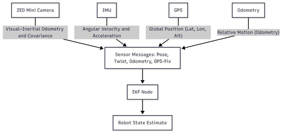
Figure 1.
Data flow among sensors.
3.1. Global Positioning System (GPS)
GPS data stands as one of the primary sources of information for localization. GPS sensors provide precise geographic coordinates, including latitude (φ), longitude (λ), and altitude (h). These parameters enable robots to pinpoint their location on the Earth’s surface. Additionally, the timestamp (t) associated with GPS data is vital for synchronization with other sensor information, allowing for robust cooperative localization.
3.2. Inertial Measurement Unit (IMU)
IMU data offers insights into the robot’s motion and orientation. IMU sensors provide measurements of linear acceleration (ax, ay, az) and angular velocity (ω) in three axes. These measurements enable robots to assess how they are moving and rotating. IMUs also provide information about the robot’s orientation, often represented as roll, pitch, and yaw angles or as quaternions. As with GPS data, the timestamp associated with IMU data is crucial for data synchronization and fusion.
3.3. Camera Odometry
Camera odometry data brings visual information into the mix, allowing robots to estimate their motion by analyzing images. Key components of camera odometry data include feature points detected or tracked in the image frame, optical flow data revealing pixel motion, and pose information representing the camera’s position and orientation. The timestamp associated with camera odometry data is essential for aligning visual information with other sensor data sources.
These sensor data types, including GPS, IMU, and camera odometry, play a pivotal role in mobile robotics, contributing to the localization, mapping, and navigation processes. The integration and fusion of data from these sensors enable robots to operate effectively in a variety of environments, from outdoor landscapes to indoor spaces, and under various conditions, including dynamic and GPS-denied scenarios. Configuration matrices for odometry data, pose data, and IMU data are provided in Table 1.

Table 1.
Configuration matrices for odometry data, pose data, and IMU data.
4. Heterogeneous Mobile Robots
4.1. Unmanned Ground Vehicle (UGV)
The UGV used in the study was equipped with a differential drive mechanism, a popular choice in mobile robotics. This type of drive system consists of two drive wheels mounted on a common axis, where each wheel can be independently driven either forward or backward. This configuration offers precise control over the robot’s motion. Notably, in this UGV, shown in Figure 2 below, its chassis and motors were sourced from an electrical wheelchair, making it a cost-effective and accessible platform for research and development.
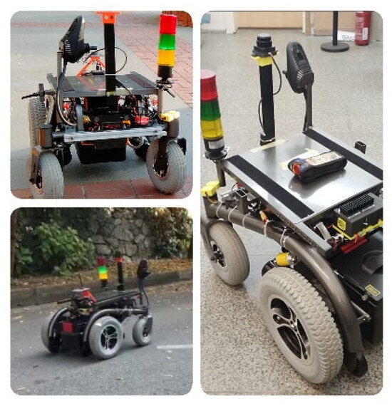
Figure 2.
Unmanned Ground Vehicle (UGV).
One of the fundamental concepts associated with differential drive systems is the concept of the Instantaneous Center of Curvature (ICC), as shown in Figure 3 below. To achieve rolling motion and enable the UGV to rotate about a specific point, the ICC comes into play. By varying the velocities of the two drive wheels, the UGV can navigate along different trajectories, and the ICC is the point around which the robot rotates during its motion.
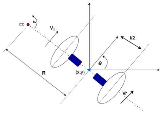
Figure 3.
Differential drive kinematics.
The equations presented above illustrate the relationship between the wheel velocities, the ICC, and rotation. Specifically, the rate of rotation () about the ICC must be the same for both wheels, leading to equations that help calculate the ICC’s location () at any given moment. These equations are crucial for understanding the robot’s movement, whether it is moving forward in a straight line, rotating in place, or rotating about one of its wheels. Additionally, the paper highlights the significance of avoiding a singularity where the UGV cannot move directly along its axis.
4.2. Unmanned Aerial Vehicle (UAV)
In the fabrication of the UAV’s arms, both the need for lightweight construction to prevent undue burden on the body and the requirement for robustness to support the rotors were considered. As a result, a composite design was employed. To construct the arms, a carbon fiber tube with an inner diameter of 16 mm and a thickness of 1 mm was fit over an aluminum tube of 1 mm thickness and 14 mm inner diameter, utilizing an interference fit method. This design leveraged the lightness of aluminum while benefiting from the strength of carbon fiber.
The use of a 3D printer was instrumental in the creation of the UAV’s landing legs, battery holder, and fasteners. The use of 3D printing enabled the formation of high-complexity fasteners according to design requirements. Furthermore, it facilitated the design of the battery holder and UAV’s landing legs with appropriate dimensions and structures. By using carbon fiber filament, structures were produced that were strong relative to their weight, and uniformly shaped. The assembly of the UAV is shown in Figure 4. The corresponding angular velocity representation about the body frame and inertial frame is indicated in Figure 5.
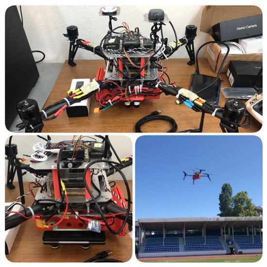
Figure 4.
Unmanned Aerial Vehicle (UAV).
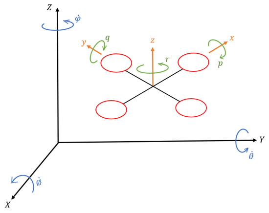
Figure 5.
Angular velocity representation about body frame and inertial frame.
The kinematics and dynamics equations can be combined as
With this, the state space equation is obtained in a very compact form. The inertia products are assumed as zero . During the mathematical model derivation of UAV, convention is employed by rotating about the moving frame. It can be given as
At this point, a special transformation matrix is needed to define the angular velocities given in the body frame with respect to an inertial frame. This special transformation matrix can be defined as
As mentioned above, convention is employed by rotating about the body frame. One of the reasons why it is selected is that finding the derivatives of the mass moments of inertias and has a high computational cost. It is more convenient to use the body frame instead of the inertial frame because of this. Therefore, dynamics equations for rotational motion regarding the body frame are used.
5. Sensor Fusion for Localization
Accurate and reliable localization is a phenomenal challenge in robotics and autonomous systems. It is imperative for robots to know their position in space in order to navigate and interact with their environment effectively. However, no single sensor can provide a complete and faultless solution to this problem. This is where sensor fusion comes into play.
Sensor fusion is a key technique that integrates data from multiple sensors to provide a more reliable and accurate understanding of a robot’s position and orientation. By combining the strengths of various sensor modalities such as GPSs, IMUs, camera odometry, and gyroscopes, sensor fusion compensates for the limitations and uncertainties of individual sensors, resulting in improved localization performance. Popular techniques in sensor fusion include Bayesian filters, Kalman filters, and particle filters.
5.1. Extended Kalman Filter (EKF)
One of the cornerstone methods employed in this study is the EKF. The EKF is a recursive estimation algorithm that extends the basic Kalman filter to handle nonlinearities in sensor measurements and dynamic systems. It is widely utilized in robotics for its capability to fuse data from sensors like GPSs, IMUs, and odometry. The EKF maintains a probability distribution of the robot’s state, effectively combining past estimates with current sensor measurements to produce a more accurate localization result. This algorithm is particularly well-suited for addressing the complexities of dynamic and noisy environments. The equations for the EKF can be divided into two main steps—the prediction step (also known as the time update) and the correction step (also known as the measurement update)—as described below with (13), (14), (15), (16), and (17).
- Prediction Step (Time Update)
The state estimate at the current time step () can be given as
Here, represents the predicted state at time , is the process model that describes how the state evolves over time, is the previous state estimate, and is the control input at time t.
The error covariance at the current time step can be written as
represents the error covariance matrix at time , is the Jacobian matrix of the process model, is the error covariance at the previous time step, and is the process noise covariance.
- 2.
- Correction Step (Measurement Update)
The Kalman gain at time t can be defined as
represents the Kalman gain at time , is the Jacobian matrix of the measurement model, and is the measurement noise covariance.
The updated state estimate at time can be expressed as
Here, is the actual measurement at time and is the measurement model that predicts what the measurement should be based on the current state estimate.
The updated error covariance at time can be provided as
Here, is the identity matrix.
5.2. Robot Operating System (ROS)
In this work, the study was conducted within the framework of the Robot Operating System (ROS). ROS is a flexible and open-source platform that is specifically designed for robotics development. It offers a comprehensive set of tools and libraries that facilitate the development, integration, and testing of robotic systems. ROS stimulates modularity. Thus, it is ideal for managing the complexities of sensor fusion and localization within a robotic application.
This study delves into the intricacies of sensor fusion, with a particular focus on the application of the EKF within the ROS platform using the ‘Robot Localization’ package. The process noise covariance () and measurement noise covariance () parameters were configured using the default settings of the ROS Robot Localization package. By combining the power of sensor fusion techniques and ROS’s capabilities, we aimed to significantly enhance the precision and reliability of cooperative localization in complex environments. This study opens the door to myriad applications in the field of robotics, including autonomous transportation, precision agriculture, and disaster response, where accurate and robust localization is crucial for mission success.
6. Trajectory Generation and Path Following
In the context of this study, we explore the use of heterogeneous mobile robots, consisting of both UAVs and UGVs, to enhance cooperative localization. Our primary objective is to improve the precision and reliability of the localization process.
The approach we employ involves a two-step procedure: waypoint collection and trajectory generation, followed by path following. First, a robot’s localization system is utilized to collect a set of crucial waypoints within the environment. These waypoints serve as reference points that guide the robots in achieving accurate positioning.
Subsequently, a trajectory is generated based on these collected waypoints. This trajectory provides a predefined path for the other robots to follow. The trajectory generation process leverages the localization information from one robot to create an optimized path that optimally suits the specific environmental conditions and cooperative localization requirements.
The trajectory generation for a drone is a sophisticated process that blends the computational capability of MATLAB R2023b with the dynamic coordination of ROS.
The foundation of trajectory generation lies in Equations (18) and (19), where represents the robot’s x-coordinate and and denote the starting and ending x-coordinates of waypoints. Also, represents the robot’s y-coordinate and and denote the starting and ending y-coordinates of waypoints. The variable signifies the timestamp associated with the starting waypoint, while corresponds to the timestamp of the ending waypoint. This equation, alongside its y-coordinate counterpart, enables us to generate a smooth trajectory between waypoints. By discretizing the data based on Euclidean distance, we ensure that the robots follow a predefined path at an appropriate velocity.
The algorithm discretizes the data. It starts from the first point and goes through the trajectory until the sum of the Euclidean distances ‘d’ exceeds the specified value. It then records that point, and the procedure is repeated. The process can be represented as shown in Figure 6. By employing the position and orientation information derived from the waypoints, alongside the Euclidean distance and trajectory velocity data, this function conducts the necessary calculations to generate the trajectory required for the UAV.
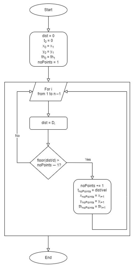
Figure 6.
Pseudocode chart representing discretization.
There is a function which is responsible for generating a set of visualizations to represent the robot’s movement in a more understandable manner. The robot’s trajectory, velocity, and acceleration in terms of linear and rotational movement while following selected waypoints are presented in Figure 7.
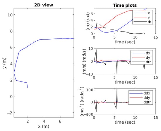
Figure 7.
Robot’s trajectory, velocity, and acceleration in terms of linear and rotational movement while following selected waypoints.
For path following, we employed a Proportional–Integral–Derivative (PID) control approach to continuously adjust the robot’s heading, allowing it to track the generated trajectory. PID control was implemented manually through a trial-and-error method. There were three PID controllers: longitudinal, lateral, and angular.
6.1. Longitudinal PID Controller
This controller primarily deals with the robot’s forward/backward motion. The longitudinal control effort () is calculated as
, , and are the proportional, integral, and derivative gains, respectively. Longitudinal error is expressed as , which measures the difference between the desired and actual positions along the robot’s longitudinal axis. Time step is expressed as , and represents the integral operation.
6.2. Lateral PID Controller
This controller primarily deals with the robot’s sideways motion. The longitudinal control effort () is calculated as
The lateral error is expressed as , which represents the difference between the desired and actual positions along the robot’s lateral axis.
6.3. Angular PID Controller
This controller focuses on controlling the robot’s orientation (heading). The angular control effort () is calculated as
Angular error is expressed as , which measures the difference between the desired and actual robot orientation.
, , and are the proportional, integral, and derivative gains for each controller, fine-tuned in MATLAB R2023b for the simulation environment. In the experimental tests, the gains for each controller were adjusted experimentally.
In practice, the trajectory generation and path following processes are implemented to ensure that all robots work collaboratively towards achieving a common goal. By following the generated trajectory, robots can maintain relative positions and coordinate their actions effectively, ultimately contributing to the enhancement of cooperative localization. Together, these techniques play a crucial role in optimizing cooperative localization, ensuring that robots navigate efficiently and accurately in dynamic environments.
This approach forms the theoretical basis for the practical implementation of trajectory generation and path following in our research, and it holds the promise of significantly improving cooperative localization in dynamic and challenging environments.
The low-level control of the UAV was managed by Pixhawk, an open-source, high-performance autopilot hardware suitable for fixed-wing, multirotor, and other platforms.
7. Simulation Setup and Results
The simulation began with the design of the UAV and UGV in Autodesk Fusion 360, a solid modeling computer-aided design and computer-aided engineering (CAE) software program. Here, the physical properties of the vehicles, such as their shape, size, and the interconnection of their parts, were defined. The CAD models were used to generate Unified Robot Description Format (URDF) models, which are XML files describing the physical properties, visual geometry, collision geometry, and kinematic properties of the robots, including their joints, links, and physical parameters like inertia tensors and centers of mass. This URDF file is crucial for ROS, as it provides a comprehensive specification of the robot’s physical aspects and how they relate to one another.
Gazebo was used to create a realistic simulation environment for the UAV and UGV. The simulation environment created in Gazebo and RViz is shown in Figure 8. These robots were tested in a risk-free, virtual world, enabling the validation of control algorithms, navigation strategies, and interaction behaviors. In the simulation, the UGV was manually controlled via keyboard inputs. Waypoints were marked during this process, which the UAV subsequently followed. As the waypoints were defined and adjusted for the UAV through the manual control of the UGV, these changes were dynamically reflected in the RViz environment.
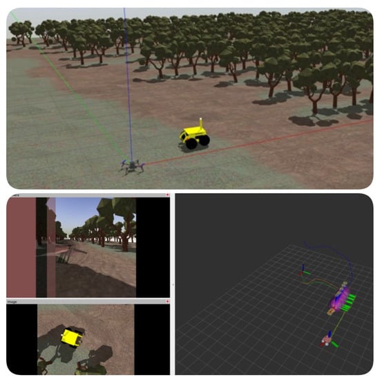
Figure 8.
Simulation environment created in Gazebo and RViz.
The UAV was controlled via MAVROS, a ROS package that provides MAVLink functionality, offering a simple and unified interface to control drones. The UAV follows the trajectory outlined by the waypoints marked by the UGV. It uses sensor data to ensure it is following the correct path. This sensor data is processed using an EKF, which is a recursive algorithm used to estimate the state of a dynamic system affected by random noise. This filtering process ensures a smooth, accurate trajectory.
In the MATLAB 2023b code, comparisons between position data derived from two different sources, one being unfiltered GPS coordinates and the other being coordinates processed by an EKF, were performed. The purpose of this was to assess the efficacy of the EKF in improving the accuracy of the position data. Position estimation with and without the EKF while the drone was following the waypoints chosen by the UGV are given in Figure 9.
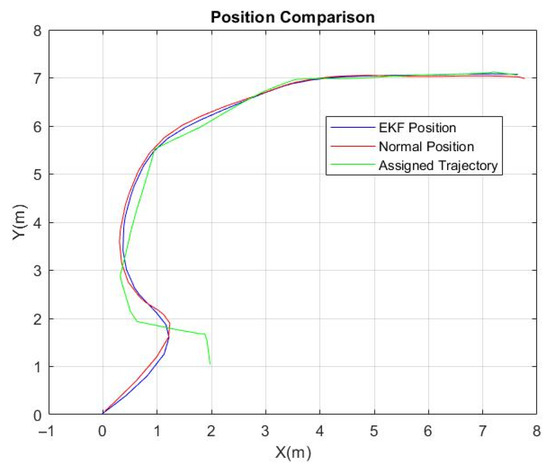
Figure 9.
Position estimation with and without Extended Kalman Filter with drone following waypoints chosen by UGV.
The final arrays contain a history of the positions reported by the GPS and EKF, respectively, each time the position changed. These arrays can be used to analyze and compare the trajectory followed by the quadrotor according to each source of position data. The EKF utilized in this scenario combined position information from Gazebo plugins, such as from the GPS, accelerometer, and magnetometer, to estimate the quadrotor’s state.
Sensor data, encompassing both unprocessed and EKF-applied measurements, were methodically tabulated and compared against a predefined trajectory, enabling an evaluation of the accuracy and dependability of tracking methodologies in dynamic environments. Erroneous or meaningless sensor measurements were eliminated using the EKF, which effectively fuses sensor data to improve accuracy. A comparative analysis of the raw and EKF-processed sensor data in waypoint navigation is provided in Table 2.
Table 2.
Comparative analysis of Raw and EKF-processed sensor data in waypoint navigation.
To further analyze the tracking accuracy, five distinct points, including their and coordinates, were selectively extracted from the graph representing the sensor data. For each of these points, the Euclidean distance from the corresponding location on the assigned trajectory was calculated. This step is crucial for quantifying the deviation of the sensor data from the expected path. The Euclidean distance is computed as
Building upon the calculated Euclidean distances, the next phase involved computing the Root Mean Square Error () to provide a comprehensive measure of the overall tracking accuracy. The offers a clear indication of the average magnitude of the tracking error across the selected points. The was calculated as
In our analysis, the Euclidean distance at each of the selected points serves as a direct measure of error, quantifying the deviation.
In our comprehensive evaluation, the performance of the drone’s navigation was meticulously assessed across various trajectory patterns, including 8-figure, ellipse, circle, hexagon, and a straight line. Position estimations with and without the EKF while the drone was following circle, hexagon-shaped, 8-figure, and ellipse-shaped trajectories are shown in Figure 10 and Figure 11. The was calculated for each trajectory pattern to quantify the tracking accuracy. An analysis of drone navigation is presented in Table 3. Five distinct points from each graph of the 8-figure, ellipse, circle, hexagon, and line patterns were selected for calculating the . Notably, the application of the EKF demonstrated a significant improvement in precision. For instance, in the assigned trajectory task, the EKF-processed data yielded an of 0.1061 m, whereas the data without EKF processing exhibited a slightly higher of 0.1416 m. These results were systematically tabulated to offer a clear comparative analysis of the drone’s tracking accuracy under different geometric patterns, underscoring the effectiveness of EKF in enhancing navigational precision.
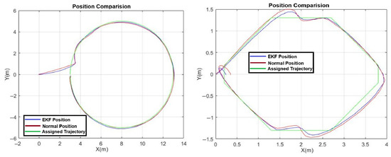
Figure 10.
Position estimation with and without Extended Kalman Filter while drone was following circle and hexagon-shaped trajectories.
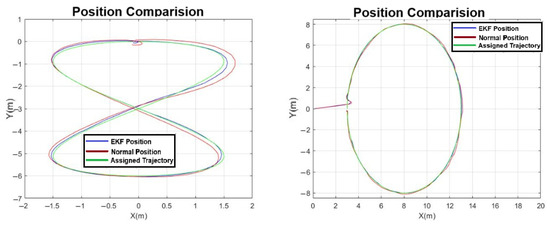
Figure 11.
Position estimation with and without Extended Kalman Filter while drone was following 8-figure and ellipse-shaped trajectory.
Table 3.
RMSE analysis of drone navigation in autonomous geometric flight modes for simulation.
While the simulation provides a reasonably realistic approximation of physical behaviors, limitations include the simplified sensor noise models and idealized communication without delays or packet loss. Nevertheless, it enabled the effective testing of localization, control logic, and system integration before deployment.
8. Experimental Test Results and Discussion
In our preliminary setup for drone assembly, the careful alignment of the rotors onto the drone arms was a critical factor. Ensuring the rotors’ flatness is paramount for optimal flight performance, as any tilt or deviation from the intended angle can cause imbalances during flight, leading to inaccurate results or crashes. To establish the precise leveling of the rotors, we employed the use of a water level ruler.
The assembly was then placed on a weighing scale, with the expectation that the downward thrust created by the spinning propeller would register as an increase in weight, effectively indicating the lifting capacity of each rotor. The experimental setup to measure the lift generated by each rotor is shown in Figure 12. The results from these tests provided valuable insight into the overall lifting capacity of the rotors, crucial information for optimizing our drone’s flight performance. Variation in lift values according to the given current under 16.3 Volts is presented in Table 4. A corresponding Amps vs. thrust diagram is provided in Figure 13.
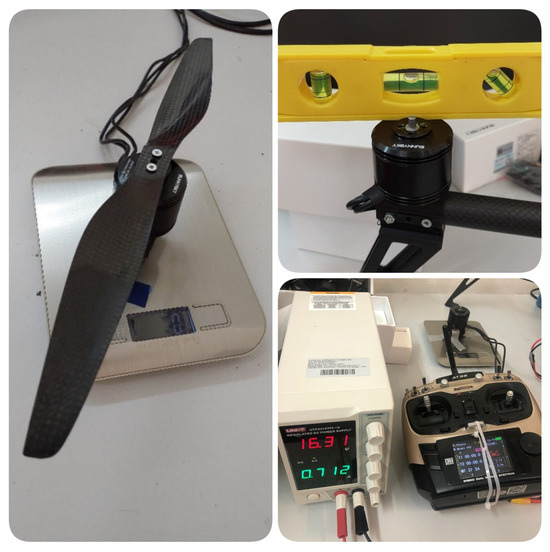
Figure 12.
Experimental setup to measure lift generated by each rotor.
Table 4.
Variation in lift values according to given current under 16.3 Volts.
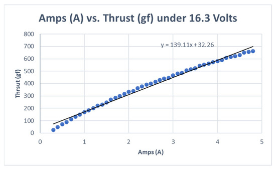
Figure 13.
Amps (A) vs. thrust (gf) under 16.3 Volts.
In the process of implementing an EKF for sensor fusion in our robotics system, we employed the ZED mini camera as a key sensor, exploiting its built-in accelerometer, gyroscope, and IMU. The ZED mini camera provides orientation information in the form of quaternions, a mathematical construct particularly useful for representing orientations and rotations of objects in three dimensions. The image view of the ZED mini camera in RViz is shown in Figure 14.
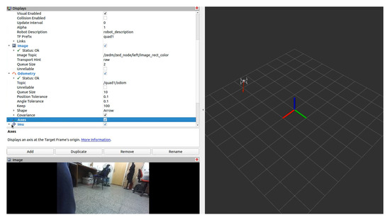
Figure 14.
Image view of ZED mini camera in RViz.
Setting up the correct configuration matrices forms a crucial part of this procedure. These matrices guide the extraction of accurate sensor information and are instrumental in their fusion within the EKF. However, defining the covariance matrices, which is a key component of the Kalman filtering process, was not handled manually. Instead, the EKF automatically integrates the covariance data derived from the ZED mini camera, thus ensuring optimal performance and reducing the risk of human-induced error. The covariance data generated by the ZED Mini is utilized to quantify uncertainty in the position and orientation estimates, which helps in improving localization accuracy by informing sensor fusion algorithms.
In this study, covariance information is utilized within the EKF during the sensor fusion process to weigh the reliability of each measurement source for both the UAV and UGV. Prior to cooperative testing, each robot was individually tested to ensure that the EKF outputs showed low covariance, indicating high confidence in the pose estimates. While the covariance contributes internally to the state estimation process, our performance evaluation focuses on the between the estimated and ground-truth positions to quantify localization accuracy. Since the objective of this work is cooperative localization rather than per-robot localization enhancement, the role of covariance is limited to its function within the filter, rather than being directly analyzed in the results.
The drone developed for this research was primarily controlled using a radio controller. During its flights, several external disturbances were encountered. Nevertheless, despite these challenges, the drone managed to hover and land safely. To evaluate the performance of the EKF, it was initially intended for the drone to undertake autonomous flight. However, this proved to be a complex endeavor due to the intricate nature of the control algorithms and trajectory-following tasks. The risk associated with ensuring control during autonomous flight rendered it an unsafe approach.
To address this limitation and still achieve data collection goals, another method was employed. The drone was controlled manually. Waypoints were generated through manual flight; there was no autonomous flight involved. The UGV was tasked with following a predefined trajectory assigned by the drone. As the UGV navigated its course, it collected sensor data and processed it through the EKF. This setup provided a valuable benchmark. The UAV’s trajectory served as a reference against which the position data derived from the UGV’s EKF could be compared. The UGV completing its task in cooperation with the UAV is shown in Figure 15. Once the UAV completes waypoint selection, it sends the waypoints to the site manager; the site manager then creates a trajectory and sends it to the UGV.
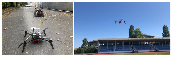
Figure 15.
The UGV was tasked with following a predefined trajectory assigned by the drone.
Moreover, for a comprehensive analysis, two sets of EKF results were charted. The first was derived from the drone’s EKF using both the ZED mini camera and GPS data, while the second omitted GPS data. EKF-applied data with and without GPS while the UGV was following the waypoints chosen by the UAV are given Figure 16. These comparative graphs effectively showcase the performance distinction between the two configurations, offering insights into the enhanced accuracy potentially achieved with the incorporation of GPS.
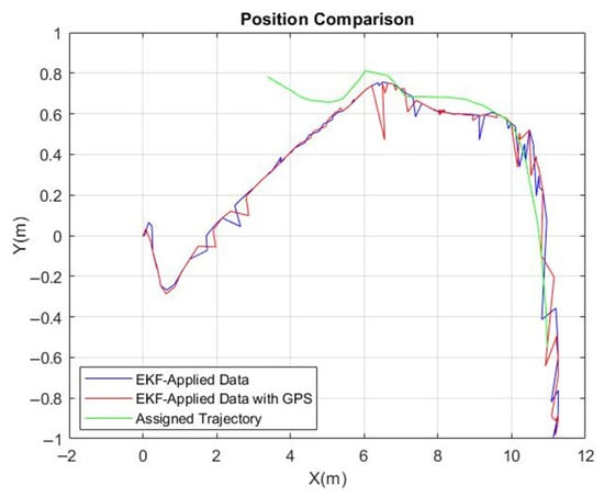
Figure 16.
EKF-applied data with and without GPS with UGV following waypoints chosen by UAV.
An enhancement in the examination of tracking precision was achieved by the meticulous selection of five specific points, along with their respective X and Y coordinates, from the chart illustrating the sensor data. The Euclidean distance to their respective positions on the predetermined path was computed for each of these points. A comparative analysis of the raw and EKF-processed sensor data with and without GPS is presented in Table 5.
Table 5.
Comparative analysis of raw and EKF-processed sensor data with and without GPS.
To enhance the granularity of our analysis, we selected five key points from each dataset’s graph, focusing on their X and Y coordinates. For these points, we calculated the Euclidean distance from the assigned trajectory, providing a precise measure of deviation. Subsequently, we computed the using these distances. Our findings revealed a notable difference in accuracy between the two methods: the EKF with GPS data resulted in an of 0.1729 m, while the EKF without GPS showed a higher of 0.2441 m. This comparison underscores the significant impact of GPS integration on the accuracy of EKF-based sensor data tracking.
In our comprehensive investigation, we expanded the scope of the analysis to include the UGV following two specific path patterns: a straight line and a U-shaped figure. EKF-applied data with and without GPS while the UGV was following the line and U-shaped trajectories are presented in Figure 17 and Figure 18. Each experiment was rigorously conducted five times to ensure consistency and reliability in our findings. The was meticulously calculated for each iteration, providing a robust dataset that reflects the UGV’s tracking precision under different conditions. This approach allowed us to observe the variability and stability of the UGV’s performance, particularly when comparing the efficacy of the EKF with and without Emlid REACH M+ GPS integration. analysis as a result of this approach is presented in Table 6.
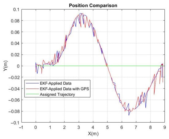
Figure 17.
The EKF-applied data with and without GPS while the UGV was following the line.
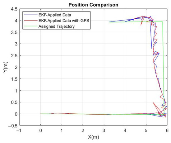
Figure 18.
The EKF-applied data with and without GPS while the UGV was following the U-shaped trajectory.
Table 6.
RMSE analysis of drone navigation in autonomous geometric flight modes.
The values from these repeated experiments have been systematically organized into a table, offering a clear and comprehensive view of the impact of path complexity and navigational aids on the UGV’s trajectory adherence. The discrepancies noted in the UGV’s trajectory adherence, indicated by the values, can be partly attributed to challenges in the autonomous control algorithm, impacting its ability to precisely follow the designated path.
9. Conclusions
In this study, the enhancement of collective movement capabilities in heterogeneous mobile robots through information sharing and data fusion was investigated. The EKF was employed for sensor fusion, focusing on improved localization accuracy.
Statistical analyses were carried out to assess the outcomes, with the integration of a cooperative localization algorithm enabling communication between quadcopters and unmanned ground vehicles.
Simulation results slightly outperformed experimental outcomes, yet the differences were not markedly significant. Notably, the implementation of the EKF with GPS consistently yielded better results compared to the EKF without GPS in object-free environments, affirming GPS’s role in enhancing navigational precision.
Furthermore, data processed with the EKF demonstrated a clear improvement over non-EKF data, indicating the efficacy of sensor fusion in robotic navigation. These findings also positively influenced the cooperative localization aspect of our research, suggesting that enhanced individual localization through EKF and GPS integration can significantly contribute to the overall improvement of cooperative navigation and coordination among heterogeneous robotic platforms.
For future work, conducting real-world experiments with autonomous drone flights presents a promising avenue. This approach would enable a more comprehensive evaluation of EKF performance in practical scenarios.
Author Contributions
Conceptualization, S.Ö.; Software, A.M.K.; Validation, A.M.K.; Writing—original draft, E.O.K.; Writing—review & editing, E.O.K.; Supervision, S.Ö.; Project administration, S.Ö. All authors have read and agreed to the published version of the manuscript.
Funding
This work was supported by the UTOPIA (Automated Open Precision Farming Platform) Project, co-funded by TUBITAK 1071 (Project No: 120N785) and the European Union’s Horizon 2020 research and innovation program under grant agreement No 862665 ERA-NET ICT-AGRI-FOOD. This work was also supported by Boğaziçi University Research Fund (Grant Number 16883) through the MARE (Multi-Agent Robot Environment) Project.
Data Availability Statement
The raw data supporting the conclusions of this article will be made available by the authors on request.
Conflicts of Interest
The authors declare no conflict of interest.
References
- Islam, N.; Rashid, M.M.; Pasandideh, F.; Ray, B.; Moore, S.; Kadel, R. A Review of Applications and Communication Technologies for Internet of Things (IoT) and Unmanned Aerial Vehicle (UAV) Based Sustainable Smart Farming. Sustainability 2021, 13, 1821. [Google Scholar] [CrossRef]
- Muchiri, G.; Kimathi, S. A Review of Applications and Potential Applications of UAV. In Proceedings of the Sustainable Research and Innovation Conference, Pretoria, South Africa, 20–24 June 2022; pp. 280–283. [Google Scholar]
- Matese, A.; Di Gennaro, S.F. Practical Applications of a Multisensor UAV Platform Based on Multispectral, Thermal and RGB High Resolution Images in Precision Viticulture. Agriculture 2018, 8, 116. [Google Scholar] [CrossRef]
- Salamí, E.; Barrado, C.; Pastor, E. UAV Flight Experiments Applied to the Remote Sensing of Vegetated Areas. Remote Sens. 2014, 6, 11051–11081. [Google Scholar] [CrossRef]
- Desai, A.; Dreossi, T.; Seshia, S.A. Combining Model Checking and Runtime Verification for Safe Robotics. In Proceedings of the Runtime Verification: 17th International Conference, Seattle, WA, USA, 13–16 September 2017; pp. 172–189. [Google Scholar]
- Lamping, A.P.; Ouwerkerk, J.N.; Cohen, K. Multi-UAV Control and Supervision with ROS. In Proceedings of the Aviation Technology, Integration, and Operations Conference, Atlanta, GA, USA, 25–29 June 2018; p. 4245. [Google Scholar]
- Garcia, S.; MLópez, E.; Barea, R.; Bergasa, L.M.; Gómez, A.; Molinos, E.J. Indoor SLAM for Micro Aerial Vehicles Control Using Monocular Camera and Sensor Fusion. In Proceedings of the International Conference on Autonomous Robot Systems and Competitions (ICARSC), Bragança, Portugal, 4–6 May 2016; pp. 205–210. [Google Scholar]
- Huang, R.; Tan, P.; Chen, B.M. Monocular Vision-Bases Autonomous Navigation System on a Toy Quadcopter in Unknown Environments. In Proceedings of the International Conference on Unmanned Aircraft Systems (ICUAS), Denver, CO, USA, 9–12 June 2015; pp. 1260–1269. [Google Scholar]
- Feng, L.; Fangchao, Q. Research on the Hardware Structure Characteristics and EKF Filtering Algorithm of the Autopilot PIXHAWK. In Proceedings of the Sixth International Conference on Instrumentation & Measurement, Computer, Communication and Control (IMCCC), Harbin, China, 21–23 July 2016; pp. 228–231. [Google Scholar]
- Bugallo, M.F.; Xu, S.; Djurić, P.M. Performance Comparison of EKF and Particle Filtering Methods for Maneuvering Targets. Digit. Signal Process. 2007, 17, 774–786. [Google Scholar] [CrossRef]
- Minaeian, S.; Liu, J.; Son, Y.J. Vision-Based Target Detection and Localization via a Team of Cooperative UAV and UGVs. IEEE Trans. Syst. Man Cybern. Syst. 2015, 46, 1005–1016. [Google Scholar] [CrossRef]
- Kurazume, R.; Nagata, S.; Hirose, S. Cooperative Positioning with Multiple Robots. In Proceedings of the IEEE International Conference on Robotics and Automation, San Diego, CA, USA, 8–13 May 1994; pp. 1250–1257. [Google Scholar]
- Rekleitis, I.; Dudek, G.; Milios, E. Multi-Robot Collaboration for Robust Exploration. Ann. Math. Artif. Intell. 2001, 31, 7–40. [Google Scholar] [CrossRef]
- Roumeliotis, S.I.; Bekey, G.A. Collective Localization: A Distributed Kalman Filter Approach to Localization of Groups of Mobile Robots. In Proceedings of the IEEE International Conference on Robotics and Automation, San Francisco, CA, USA, 24–28 April 2000; Volume 3, pp. 2958–2965. [Google Scholar]
- Nerurkar, E.D.; Roumeliotis, S.I.; Martinelli, A. Distributed Maximum a Posteriori Estimation for Multi-Robot Cooperative Localization. In Proceedings of the IEEE International Conference on Robotics and Automation, Kobe, Japan, 12–17 May 2009; pp. 1402–1409. [Google Scholar]
- Ahmadinia, M.; Alinejad-Rokny, H.; Ahangarikiasari, H. Data Aggregation in Wireless Sensor Networks Based on Environmental Similarity: A Learning Automata Approach. J. Netw. 2014, 9, 2567. [Google Scholar] [CrossRef]
- Karam, N.; Chausse, F.; Aufrere, R.; Chapuis, R. Localization of a Group of Communicating Vehicles by State Exchange. In Proceedings of the IEEE/RSJ International Conference on Intelligent Robots and Systems, Beijing, China, 9–15 October 2006; pp. 519–524. [Google Scholar]
- Prorok, A.; Bahr, A.; Martinoli, A. Low-Cost Collaborative Localization for Large-Scale Multi-Robot Systems. In Proceedings of the IEEE International Conference on Robotics and Automation, Saint Paul, MN, USA, 14–18 May 2012; pp. 4236–4241. [Google Scholar]
- Mourikis, A.I.; Roumeliotis, S.I. Performance Analysis of Multirobot Cooperative Localization. IEEE Trans. Robot. 2006, 22, 666–681. [Google Scholar] [CrossRef]
- Julier, S.J.; Uhlmann, J.K. A Non-Divergent Estimation Algorithm in the Presence of Unknown Correlations. In Proceedings of the American Control Conference, Albuquerque, NM, USA, 6 June 1997; Volume 4, pp. 2369–2373. [Google Scholar]
- Carillo-Arce, L.C.; Nerurkar, E.D.; Gordillo, J.L.; Roumeliotis, S.I. Decentralized Multi-Robot Cooperative Localization Using Covariance Intersection. In Proceedings of the IEEE/RSJ International Conference on Intelligent Robot and Systems, Tokyo, Japan, 3–7 November 2013; pp. 1412–1417. [Google Scholar]
Disclaimer/Publisher’s Note: The statements, opinions and data contained in all publications are solely those of the individual author(s) and contributor(s) and not of MDPI and/or the editor(s). MDPI and/or the editor(s) disclaim responsibility for any injury to people or property resulting from any ideas, methods, instructions or products referred to in the content. |
© 2025 by the authors. Licensee MDPI, Basel, Switzerland. This article is an open access article distributed under the terms and conditions of the Creative Commons Attribution (CC BY) license (https://creativecommons.org/licenses/by/4.0/).