Robust Predictive Functional Control for Quadrotor Flight Systems

Abstract

Predictive Functional Control (PFC) has a control structure similar to Model Predictive Control (MPC), determining control inputs by predicting future states using a motion model. However, PFC does not require solving a quadratic programming problem for every control loop like MPC. This feature enables PFC to be implemented in small-scale systems such as actuators, where embedding a high-performance computer is difficult. However, similar to MPC, there are concerns with PFC regarding control performance degradation due to incorrect predictions of future states in environments affected by modeling errors and disturbances. Therefore, in this study, we propose a novel method that employs robustness, Robust Predictive Functional Control (RPFC). The proposed RPFC method was applied to a quadrotor flight control system, and its effectiveness was verified through numerical simulations. Specifically, the control performance of RPFC under disturbance conditions was compared with that of conventional PFC, demonstrating the advantages of the proposed approach.

1. Introduction

Model Predictive Control (MPC) is a control strategy that predicts future system states using a dynamic motion model [1,2,3,4,5,6,7,8,9,10]. It determines optimal control inputs by minimizing a predefined evaluation function, which typically includes terms representing tracking errors relative to a reference trajectory, as well as control effort. Unlike classical control methods, MPC is expected to see expanded use in industrial systems [1,2,3] owing to its ability to handle constraints on actuators and system states while enabling the intuitive design of transient responses in the time domain. However, a well-known drawback of MPC lies in its control structure, which requires solving sequential optimization problems and results in a significantly higher computational load than conventional controllers such as PID. This issue is not critical in applications such as chemical plants, where system dynamics evolve slowly and sufficient computation time is available. However, it poses a significant challenge for systems with stringent real-time requirements, such as aircraft. For instance, although Unmanned Aerial Vehicle (UAV) applications of MPC have been explored [6,7,8], validation has been limited to numerical simulations. In [9,10], flight experiments were conducted by computing the control inputs on a desktop personal computer using telemetry data from a UAV. However, this approach limits the operational flight area due to the communication range and makes it difficult to maintain flight if communication failures occur. Furthermore, in low-level control systems where control inputs must be computed onboard, such as actuator-level servo control in cascade control architectures, implementing MPC remains difficult. Therefore, applying high computational load controllers like MPC to low-level control systems, such as those for aircraft and actuators, presents unresolved challenges. To address this limitation, Predictive Functional Control (PFC) [11,12,13,14,15,16,17,18] has been proposed as an alternative approach that reduces the computational load associated with MPC.

While MPC determines control inputs to minimize the error between the reference trajectory and the predicted trajectory over a predefined prediction horizon from the current time, PFC determines inputs to minimize the error at a specific coincidence point between the reference and predicted trajectories. Due to its control structure, PFC inherits similar advantages to MPC, such as intuitive adjustment of transient responses, while keeping a low computational load. As a result, it is expected to replace the PID control and is applicable in systems such as linear servo systems [16,17]. However, PFC predicts future states based on internal motion models like MPC, raising concerns about potential deterioration in control performance due to disturbances such as modeling errors and unexpected external forces. To address this problem, methods involving the introduction of a disturbance observer [16,17,18] have been proposed, leading to improvements in control performance under the influence of disturbances. This approach requires a separate design for both PFC and a disturbance observer, complicating the control system’s structure.

To address the limitations of conventional approaches, this study proposes a novel control method that incorporates the concept of Sliding Mode Control (SMC) [19,20,21,22,23,24,25]. SMC is a control strategy that constrains system states to a hypersurface in phase space using a switching function. Due to its simple structure and strong robustness against model uncertainties and external disturbances, SMC has been combined with MPC in several previous studies [26,27,28,29,30]. Among the various types of SMC, Integral Sliding Mode Control (ISMC) is particularly suitable for combination with MPC. By constraining the system states to a hypersurface, ISMC allows the dynamics of a disturbed system to approximate that of a nominal system. Even under the influence of disturbances, ISMC can reduce the discrepancy between the predicted future states in MPC and the actual system states, thereby mitigating the degradation of control performance typically observed in MPC under such conditions. Accordingly, several approaches combining ISMC and MPC have been proposed [26,27]. Moreover, various robust predictive control approaches that incorporate SMC concepts have been proposed. For example, in Model Predictive Sliding Mode Control (MPSMC) [28,29,30], the switching function is predicted based on an internal model, and the control input is determined through an evaluation function. Similarly, Extended Model Predictive Control (EMPC) [31,32] and Robust Monte Carlo Model Predictive Control (RMCMPC) [33] employ predictive models that simultaneously estimate the switching function and nominal system states to determine control actions. These controllers have demonstrated excellent robustness, but as with general MPC, the computational load remains a non-negligible issue. To address this challenge, we propose a new control method called Robust Predictive Functional Control (RPFC), which simultaneously achieves robustness and low computational load. The RPFC determines the control input by minimizing the prediction error at specific coincidence points between the reference trajectory and the predicted system states, as well as between the hypersurface and the predicted switching function. The control input can be computed through matrix addition, subtraction, and inner products, and the coefficient matrices required for input computation can be calculated offline. Therefore, as with PFC, RPFC is particularly well suited for systems with limited computational resources or those requiring short control cycles. While retaining the advantages of PFC, RPFC enhances robustness by constraining the system states toward a hyperplane in a manner comparable to techniques such as EMPC and RMCMPC. Unlike conventional disturbance observers that require information such as the frequency characteristics of the disturbance for controller design, the proposed control structure enables the design process without relying on such information. Furthermore, RPFC evaluates the state variables in the phase space, enabling the system to maintain its dynamic behavior close to the nominal performance even under the influence of disturbances. This is in contrast to conventional PID control, where external disturbances can affect transient response. The proposed RPFC is expected to improve tracking performance under such conditions due to its ability to preserve nominal-like transient characteristics despite the presence of disturbances. The combination of low computational load, robustness against unknown disturbances, and improved tracking under disturbance conditions makes RPFC a promising solution for control systems in UAVs such as quadrotors. In this study, the proposed RPFC is applied to the flight control system of a quadrotor to evaluate its effectiveness. We provide a detailed explanation of how RPFC and conventional PFC are implemented in the quadrotor system. Performance evaluation is conducted through numerical simulations, in which the control performance of both controllers is compared under nominal conditions and various types of disturbances.

2. Control Theory

This section provides a detailed explanation of both conventional Predictive Functional Control (PFC) and the Robust Predictive Functional Control (RPFC) proposed in this study. First, the following subsection defines the dynamic system.

2.1. Problem Statement

Conventional PFC is designed for discrete-time, linear time-invariant systems, which can be represented by the following equations [1,11,12].

$$\mathbf{x}\left(k+1\right)=\mathbf{A}\mathbf{x}\left(k\right)+\mathbf{B}\mathbf{u}\left(k\right)$$

(1)

$$\mathbf{y}\left(k\right)=\mathbf{C}\mathbf{x}\left(k\right)$$

(2)

This system is an $m$-input, $m$-output, $n$-dimensional state-space system, in which the dimensions of the input and output are identical. $k$ represents a specific time step; $\mathbf{u}\left(k\right)\in {\mathbb{R}}^m$ denotes the input vector at time step $k$; $\mathbf{y}\left(k\right)\in {\mathbb{R}}^m$ represents the output vector; and $\mathbf{x}\left(k\right)\in {\mathbb{R}}^n$ is the state vector, where $\mathbb{R}$ is a set consisting of the whole real numbers. Matrices $\mathbf{A}\in {\mathbb{R}}^{n\times n}$, $\mathbf{B}\in {\mathbb{R}}^{n\times m}$, and $\mathbf{C}\in {\mathbb{R}}^{m\times n}$ are coefficient matrices.

In practice, however, modeling errors, parameter variations, and external disturbances can affect the system, causing deviations from the nominal model in Equation (1). Considering such disturbances, the system can be rewritten as

$$\mathbf{x}\left(k+1\right)=\left(\mathbf{A}+∆\mathbf{A}\left(k\right)\right)\mathbf{x}\left(k\right)+\left(\mathbf{B}+∆\mathbf{B}\left(k\right)\right)\mathbf{u}\left(k\right)+\mathbf{d}\left(\mathbf{x},k\right)$$

(3)

where $\mathsf{\Delta }\mathbf{A}\left(k\right)\in {\mathbb{R}}^{n\times n}$ and $\mathsf{\Delta }\mathbf{B}\left(k\right)\in {\mathbb{R}}^{n\times m}$ represent parameter variations in matrices $\mathbf{A}$ and $\mathbf{B}$, respectively, while $\mathbf{d}\left(\mathbf{x},k\right)\in {\mathbb{R}}^n$ denotes the disturbance vector. It is assumed that all parameter variations and disturbances can be additively applied to the input. These effects can be expressed using virtual inputs as follows:

$$∆\mathbf{A}\left(k\right)\mathbf{x}\left(k\right)=\mathbf{B}{\mathbf{u}}_A\left(k\right)$$

(4)

$$∆\mathbf{B}\left(k\right)\mathbf{u}\left(k\right)=\mathbf{B}{\mathbf{u}}_B\left(k\right)$$

(5)

$$\mathbf{d}\left(\mathbf{x},k\right)=\mathbf{B}{\mathbf{u}}_d\left(\mathbf{x},k\right)$$

(6)

${\mathbf{u}}_A\left(k\right)$ and ${\mathbf{u}}_B\left(k\right)$ represent virtual inputs that account for variations in system matrices $∆\mathbf{A}\left(k\right)$ and $∆\mathbf{B}\left(k\right)$, respectively, while ${\mathbf{u}}_d\left(\mathbf{x},k\right)$ denotes a virtual input that represents the force of external disturbances. The combined force of these virtual inputs is defined as ${\mathbf{u}}_h\left(\mathbf{x},k\right)$, which is denoted by

$${\mathbf{u}}_h\left(\mathbf{x},k\right)={\mathbf{u}}_A\left(k\right)+{\mathbf{u}}_B\left(k\right)+{\mathbf{u}}_d\left(\mathbf{x},k\right)$$

(7)

Then, the state equation represented by Equation (3) becomes

$$\mathbf{x}\left(k+1\right)=\mathbf{A}\mathbf{x}\left(k\right)+\mathbf{B}\mathbf{u}\left(k\right)+\mathbf{B}{\mathbf{u}}_h\left(\mathbf{x},k\right)$$

(8)

In other words, the parameter variations and input disturbances of the system in Equation (3) are assumed to satisfy matching conditions. This study proposes a robust controller for systems with parameter variations and external forces that satisfy these matching conditions, as represented by Equation (3).

2.2. Predictive Functional Control (PFC)

Similarly to MPC, PFC is a control method that predicts future outputs based on a dynamical model of the target system and determines control inputs accordingly. In general, when no estimator is used, such as a disturbance observer, the disturbance term represented by Equation (8) is unknown. Therefore, the internal model used for prediction is typically based on the ideal, disturbance-free system described in Equation (1). For this ideal model, the predicted state vector, $\widehat{\mathbf{x}}\left(k+i|k\right)$, at step $i$ from the current time step, $k$, is expressed as

$$\widehat{\mathbf{x}}\left(k+i|k\right)={\mathbf{A}}^i\mathbf{x}\left(k\right)+\left[\begin{array}{cccc}{\mathbf{A}}^{i-1}\mathbf{B}& {\mathbf{A}}^{i-2}\mathbf{B}& \cdots & \mathbf{B}\end{array}\right]\left[\begin{array}{c}\widehat{\mathbf{u}}\left(k|k\right)\\ \widehat{\mathbf{u}}\left(k+1|k\right)\\ ⋮\\ \widehat{\mathbf{u}}\left(k+i-1|k\right)\end{array}\right]$$

(9)

where $\widehat{\mathbf{u}}$ represents the future input. Based on Equation (2), the predicted output $\widehat{\mathbf{y}}\left(k+i|k\right)$ is denoted by

$$\widehat{\mathbf{y}}\left(k+i|k\right)=\mathbf{C}\widehat{\mathbf{x}}\left(k+i|k\right)$$

(10)

Substituting the predicted state vector, $\widehat{\mathbf{x}}\left(k+i|k\right)$, provided in Equation (9), we obtain the predicted output using the following equation.

$$\widehat{\mathbf{y}}\left(k+i|k\right)=\mathbf{C}{\mathbf{A}}^i\mathbf{x}\left(k\right)+\left[\begin{array}{cccc}\mathbf{C}{\mathbf{A}}^{i-1}\mathbf{B}& \mathbf{C}{\mathbf{A}}^{i-2}\mathbf{B}& \cdots & \mathbf{C}\mathbf{B}\end{array}\right]\left[\begin{array}{c}\widehat{\mathbf{u}}\left(k|k\right)\\ \widehat{\mathbf{u}}\left(k+1|k\right)\\ ⋮\\ \widehat{\mathbf{u}}\left(k+i-1|k\right)\end{array}\right]$$

(11)

PFC utilizes this prediction equation and expresses the terms related to the control input using basis functions

$$\sum _{j=1}^i\mathbf{C}{\mathbf{A}}^{j-1}\mathbf{B}\widehat{\mathbf{u}}\left(k+j-1|k\right)={\mathsf{\beta }}_0\left(i\right){\mathsf{\mu }}_0\left(k\right)+{\mathsf{\beta }}_1\left(i\right){\mathsf{\mu }}_1\left(k\right)+{\mathsf{\beta }}_2\left(i\right){\mathsf{\mu }}_2\left(k\right)$$

(12)

The first term on the right-hand side of Equation (12) corresponds to the zeroth-order input with respect to time, the second term corresponds to the first-order input, and the third to the second-order input. The terms ${\mathsf{\mu }}_0\left(k\right)$, ${\mathsf{\mu }}_1\left(k\right)$, and ${\mathsf{\mu }}_2\left(k\right)$ are unknown input coefficients. The input matrices ${\mathsf{\beta }}_0\left(i\right)$, ${\mathsf{\beta }}_1\left(i\right)$, and ${\mathsf{\beta }}_2\left(i\right)$, corresponding to the $i$-th prediction from time step $k$, are denoted by

$${\mathsf{\beta }}_0\left(i\right)=\left[\begin{array}{cccc}\mathbf{C}{\mathbf{A}}^{i-1}\mathbf{B}& \mathbf{C}{\mathbf{A}}^{i-2}\mathbf{B}& \cdots & \mathbf{C}\mathbf{B}\end{array}\right]\left[\begin{array}{c}{\mathbf{I}}_m\\ {\mathbf{I}}_m\\ ⋮\\ {\mathbf{I}}_m\end{array}\right]$$

(13)

$${\mathsf{\beta }}_1\left(i\right)=\left[\begin{array}{cccc}\mathbf{C}{\mathbf{A}}^{i-1}\mathbf{B}& \mathbf{C}{\mathbf{A}}^{i-2}\mathbf{B}& \cdots & \mathbf{C}\mathbf{B}\end{array}\right]\left[\begin{array}{c}{0}_m\\ ∆t{\mathbf{I}}_m\\ ⋮\\ \left(i-1\right)∆t{\mathbf{I}}_m\end{array}\right]$$

(14)

$${\mathsf{\beta }}_2\left(i\right)=\left[\begin{array}{cccc}\mathbf{C}{\mathbf{A}}^{i-1}\mathbf{B}& \mathbf{C}{\mathbf{A}}^{i-2}\mathbf{B}& \cdots & \mathbf{C}\mathbf{B}\end{array}\right]\left[\begin{array}{c}{0}_m\\ ∆t^2{\mathbf{I}}_m\\ ⋮\\ {\left(\left(i-1\right)∆t\right)}^2{\mathbf{I}}_m\end{array}\right]$$

(15)

where $∆t$ denotes the sampling time, $0_m$ is the $m\times m$ zero matrix, and ${\mathbf{I}}_m$ is the $m\times m$ identity matrix. Consequently, when the control input is represented using basis functions, the predicted output, $\widehat{\mathbf{y}}\left(k+i|k\right)$, at the $i$-th step from time $k$ becomes

$$\widehat{\mathbf{y}}\left(k+i|k\right)=\mathbf{C}{\mathbf{A}}^i\mathbf{x}\left(k\right)+{\mathsf{\beta }}_0\left(i\right){\mathsf{\mu }}_0\left(k\right)+{\mathsf{\beta }}_1\left(i\right){\mathsf{\mu }}_1\left(k\right)+{\mathsf{\beta }}_2\left(i\right){\mathsf{\mu }}_2\left(k\right)$$

(16)

Next, the reference trajectory, $\mathbf{r}$, in PFC is defined as follows:

$$\mathbf{r}\left(k+i\right)=\left({\mathbf{y}}_c\left(k\right)-\mathbf{y}\left(k\right)\right)\lambda \left(i\right)$$

(17)

In this equation, ${\mathbf{y}}_c\left(k\right)$ is the command value, and $\lambda \left(i\right)$ is defined as

$$\lambda \left(i\right)=\left(1-e^{-\left(\Delta t/T\right)i}\right)$$

(18)

The function $\lambda \left(i\right)$ determines the time response of the deviation and can be freely designed by the control engineer as a tunable parameter within the controller design process [11,12]. This study adopts an exponential function of time, which is commonly used. In Equation (18), $T$ is the time constant, which serves as a design parameter for adjusting the response of the system to the command value. Assuming that the predicted output and the predicted switching function coincide with their respective reference trajectories at three points, the following equation can be formulated:

$$\left[\begin{array}{c}\mathbf{r}\left(k+i_1\right)\\ \mathbf{r}\left(k+i_2\right)\\ \mathbf{r}\left(k+i_3\right)\end{array}\right]=\left[\begin{array}{c}\mathbf{C}{\mathbf{A}}^{i_1}\\ \mathbf{C}{\mathbf{A}}^{i_2}\\ \mathbf{C}{\mathbf{A}}^{i_3}\end{array}\right]\mathbf{x}\left(k\right)+\mathsf{\beta }\left(i_1,i_2,i_3\right)\left[\begin{array}{c}{\mathsf{\mu }}_0\left(k\right)\\ {\mathsf{\mu }}_1\left(k\right)\\ {\mathsf{\mu }}_2\left(k\right)\end{array}\right]-\left[\begin{array}{c}\mathbf{y}\left(k\right)\\ \mathbf{y}\left(k\right)\\ \mathbf{y}\left(k\right)\end{array}\right]$$

(19)

where $i_1$, $i_2$, and $i_3$ represent the number of samples from time step $k$ to the $i_1$, $i_2$, and $i_3$-th coincidence point between the ideal model and reference trajectory, $\mathsf{\beta }\left(i_1,i_2,i_3\right)$ are expressed as follows:

$$\mathsf{\beta }\left(i_1,i_2,i_3\right)=\left[\begin{array}{ccc}{\mathsf{\beta }}_0\left(i_1\right)& {\mathsf{\beta }}_1\left(i_1\right)& {\mathsf{\beta }}_2\left(i_1\right)\\ {\mathsf{\beta }}_0\left(i_2\right)& {\mathsf{\beta }}_1\left(i_2\right)& {\mathsf{\beta }}_2\left(i_2\right)\\ {\mathsf{\beta }}_0\left(i_3\right)& {\mathsf{\beta }}_1\left(i_3\right)& {\mathsf{\beta }}_2\left(i_3\right)\end{array}\right]$$

(20)

In this study, the number of coincidence points in the PFC is set to three, but it is also possible to select a different number. Increasing the number of coincidence points provides more locations at which the error between the reference and predicted trajectory is evaluated. This leads to a higher-order control input and potentially improves control accuracy. However, it also increases the computational burden. Therefore, in this study, the number of coincidence points is set to three as a compromise between control performance and computational complexity.

Using Equation (19) and solving for the unknown input coefficients, we derive the following equation.

$$\left[\begin{array}{c}{\mathsf{\mu }}_0\left(k\right)\\ {\mathsf{\mu }}_1\left(k\right)\\ {\mathsf{\mu }}_2\left(k\right)\end{array}\right]={\mathsf{\beta }}^{-1}\left(i_1,i_2,i_3\right)\left(\left[\begin{array}{c}\mathbf{r}\left(k+i_1\right)\\ \mathbf{r}\left(k+i_2\right)\\ \mathbf{r}\left(k+i_3\right)\end{array}\right]-\left[\begin{array}{c}\mathbf{C}{\mathbf{A}}^{i_1}\\ \mathbf{C}{\mathbf{A}}^{i_2}\\ \mathbf{C}{\mathbf{A}}^{i_3}\end{array}\right]\mathbf{x}\left(k\right)+\left[\begin{array}{c}\mathbf{y}\left(k\right)\\ \mathbf{y}\left(k\right)\\ \mathbf{y}\left(k\right)\end{array}\right]\right)$$

(21)

In this formulation, it is necessary to compute the inverse of matrix $\mathsf{\beta }$, which must be a nonsingular matrix. Matrix $\mathsf{\beta }$ is determined by the selection of coincidence points $i_1$, $i_2$, and $i_3$; system matrices $\mathbf{A}$, $\mathbf{B}$, and $\mathbf{C}$; and the sampling time, $\mathsf{\Delta }t$. In other words, the computation of $\mathsf{\beta }$, the verification of its rank, and the calculation of its inverse can all be performed offline in advance. As observed from the block structure of Equation (20), if $i_1=i_2=i_3$ (or $i_1=i_2\ne i_3$, $i_1\ne i_2=i_3$, $i_1=i_3\ne i_2$), the row elements of the block matrix corresponding to each coincidence point become identical, resulting in a rank-deficient $\mathsf{\beta }$. In such a case, $\mathsf{\beta }$ becomes singular, and its inverse does not exist. Therefore, it is essential to ensure that the coincidence points are selected such that $i_1\ne i_2\ne i_3$ to maintain the regularity of $\mathsf{\beta }$. Based on the above discussion, once the matrix $\mathsf{\beta }$ has been appropriately defined and its inverse computed, Equation (21) can be calculated to determine the basis function input coefficients ${\mathsf{\mu }}_0\left(k\right)$, ${\mathsf{\mu }}_1\left(k\right)$, and ${\mathsf{\mu }}_2\left(k\right)$. The input becomes $\mathbf{0}$ for the first- and second-order terms with respect to time at time step $k$. The control input can be represented solely by the zeroth-order terms, ${\mathsf{\mu }}_0\left(k\right)$, as follows:

$$\mathbf{u}\left(k\right)=\left[\begin{array}{ccc}{\mathbf{I}}_m& {\mathbf{0}}_m& {\mathbf{0}}_m\end{array}\right]\left[\begin{array}{c}{\mathsf{\mu }}_0\left(k\right)\\ {\mathsf{\mu }}_1\left(k\right)\\ {\mathsf{\mu }}_2\left(k\right)\end{array}\right]={\mathbf{I}}_u\left[\begin{array}{c}{\mathsf{\mu }}_0\left(k\right)\\ {\mathsf{\mu }}_1\left(k\right)\\ {\mathsf{\mu }}_2\left(k\right)\end{array}\right]$$

(22)

where ${\mathbf{I}}_u$ is the input coefficient matrix used to extract the zeroth-order terms ${\mathsf{\mu }}_0\left(k\right)$. Finally, the block diagram of the PFC is shown in Figure 1.

2.3. Robust Predictive Functional Control (RPFC)

In this subsection, we will explain Robust Predictive Functional Control (RPFC) in detail. RPFC improves robustness while maintaining the simple control structure of PFC. The proposed RPFC determines the control input using the following equation.

$$\mathbf{u}\left(k\right)={\mathbf{u}}_0\left(k\right)+{\mathbf{u}}_1\left(k\right)$$

(23)

where ${\mathbf{u}}_0\left(k\right)$ is the control input for the ideal system without disturbances, as denoted by the equation.

$$\mathbf{x}\left(k+1\right)=\mathbf{A}\mathbf{x}\left(k\right)+\mathbf{B}{\mathbf{u}}_0\left(k\right)$$

(24)

The input ${\mathbf{u}}_1\left(k\right)$ in Equation (23) is the control input to suppress disturbances and determine the input to constrain the system’s state variables to a hypersurface. In this way, RPFC improves the robustness of PFC by constraining the state variables to a designed hypersurface similar to SMC [19,20,21,22,23,24,25,26].

First, the switching function, $\mathsf{\sigma }\left(k\right)$, used in RPFC is defined with the following structure, similar to ISMC [21,22,23].

$$\mathsf{\sigma }\left(k\right)=\mathbf{S}\mathbf{x}\left(k\right)-\mathbf{z}\left(k\right)$$

(25)

where $\mathbf{S}\in {\mathbb{R}}^{m\times n}$ represents the coefficient matrix of switching hypersurface $\mathbf{S}\mathbf{x}\left(k\right)$, and $\mathbf{z}\left(k\right)$ is defined as follows:

$$\mathbf{z}\left(k+1\right)=\mathbf{z}\left(k\right)+\mathbf{S}\left(\left(\mathbf{A}-{\mathbf{I}}_n\right)\mathbf{x}\left(k\right)+\mathbf{B}{\mathbf{u}}_0\left(k\right)\right)$$

(26)

${\mathbf{I}}_n$ is an $n\times n$ identity matrix. In conventional SMC, the switching function is composed solely of switching hypersurface $\mathbf{S}\mathbf{x}\left(k\right)$, but in RPFC, similar to ISMC, an auxiliary variable, $\mathbf{z}\left(k\right)$, is introduced in the switching function. The initial value of the auxiliary variable, $\mathbf{z}\left(0\right)$, is set to $\mathbf{S}\mathbf{x}\left(0\right)$. The design of the switching hypersurface can be achieved using methods proposed in conventional SMC, such as eigenvalue placement [24] or optimal hypersurface design techniques that minimize a quadratic evaluation function [25].

Next, we consider the case where the switching function defined by Equation (25) is $\mathbf{0}$, in other words, where the state variables of the system are bound by the hypersurface. This condition can be expressed as

$$\mathsf{\sigma }\left(k\right)=\mathsf{\sigma }\left(k+1\right)=\mathbf{0}$$

(27)

Substituting Equation (25) into Equation (27), we obtain

$$\mathsf{\sigma }\left(k+1\right)-\mathsf{\sigma }\left(k\right)=\mathbf{S}\mathbf{x}\left(k+1\right)-\mathbf{z}\left(k+1\right)-\mathbf{S}\mathbf{x}\left(k\right)+\mathbf{z}\left(k\right)=\mathbf{0}$$

(28)

When the control input provided by Equation (23) is applied to the system with disturbances described in Equation (8), Equation (28) becomes

$$\mathbf{S}\left(\mathbf{A}\mathbf{x}\left(k\right)+\mathbf{B}{\mathbf{u}}_0\left(k\right)+\mathbf{B}{\mathbf{u}}_1\left(k\right)+\mathbf{B}{\mathbf{u}}_h\left(\mathbf{x},k\right)\right)-\mathbf{z}\left(k\right)-\mathbf{S}\left(\left(\mathbf{A}-{\mathbf{I}}_n\right)\mathbf{x}\left(k\right)+\mathbf{B}{\mathbf{u}}_0\left(k\right)\right)-\mathbf{S}\mathbf{x}\left(k\right)+\mathbf{z}\left(k\right)=\mathbf{0}$$

(29)

Rearranging, we obtain the relationship

$${\mathbf{u}}_1\left(k\right)=-{\mathbf{u}}_h\left(\mathbf{x},k\right)$$

(30)

For the system defined by Equation (8), when the control input from Equation (23) is applied to the equation

$$\mathbf{x}\left(k+1\right)=\mathbf{A}\mathbf{x}\left(k\right)+\mathbf{B}{\mathbf{u}}_0\left(k\right)+\mathbf{B}{\mathbf{u}}_1\left(k\right)+\mathbf{B}{\mathbf{u}}_h\left(\mathbf{x},k\right)$$

(31)

and the relational expression derived from Equation (30) is substituted, the equation becomes

$$\mathbf{x}\left(k+1\right)=\mathbf{A}\mathbf{x}\left(k\right)+\mathbf{B}{\mathbf{u}}_0\left(k\right)$$

(32)

Thus, if the state variables of the system are constrained to the hypersurface and the relationship described by Equation (30) is satisfied, the system behaves identically to the ideal system described by Equation (24). By converging the switching function to $\mathbf{0}$, the influence of disturbances, ${\mathbf{u}}_h\left(\mathbf{x},k\right)$, can be suppressed, and the system can approach the ideal response under the influence of disturbance. The characteristics obtained from this approach are the same as those of ISMC in discrete time; however, the RPFC proposed in this study differs from ISMC in how control input ${\mathbf{u}}_0$, which determines the ideal response, and control input ${\mathbf{u}}_1$, which suppresses disturbances, are determined. In RPFC, inputs ${\mathbf{u}}_0$ and ${\mathbf{u}}_1$ are determined by predicting the response based on the model of the control system. By contrast, in general SMC and ISMC, the control input is determined using a sign function, which leads to the issue of input oscillation, commonly known as chattering. RPFC avoids chattering by not using a sign function in input determination. Furthermore, because the response can be shaped by the reference trajectory in the time domain without being influenced by the switching hypersurface, the transient response can be designed intuitively. The next paragraph will provide a detailed explanation of the methods used to determine inputs ${\mathbf{u}}_0$ and ${\mathbf{u}}_1$ in RPFC.

In RPFC, similar to PFC, the system response is predicted based on the model, and in addition to determining the input that realizes the ideal response, the input required to make the switching function converge to 0 is also determined. For this purpose, the output, $\mathbf{y}$, and the switching function, $\mathsf{\sigma }$, are predicted based on the ideal model. Firstly, the predicted future output, $\widehat{\mathbf{y}}\left(k+i|k\right)$, from time step $k$ to $k+i$ is expressed as

$$\widehat{\mathbf{y}}\left(k+i|k\right)=\mathbf{C}{\mathbf{A}}^i\mathbf{x}\left(k\right)+\left[\begin{array}{cccc}\mathbf{C}{\mathbf{A}}^{i-1}\mathbf{B}& \mathbf{C}{\mathbf{A}}^{i-2}\mathbf{B}& \cdots & \mathbf{C}\mathbf{B}\end{array}\right]\left[\begin{array}{c}{\widehat{\mathbf{u}}}_0\left(k|k\right)\\ {\widehat{\mathbf{u}}}_0\left(k+1|k\right)\\ ⋮\\ {\widehat{\mathbf{u}}}_0\left(k+i-1|k\right)\end{array}\right]$$

(33)

The prediction of the output, $\widehat{\mathbf{y}}$, is based solely on the future control inputs, ${\widehat{\mathbf{u}}}_0$, applied to the ideal model, assuming that input ${\mathbf{u}}_1$ effectively suppresses disturbances, resulting in the system response provided by Equation (24), where ${\mathbf{u}}_1$ does not influence the transient response. Next, the prediction of the switching function, $\mathsf{\sigma }$, is explained. The predicted value of $\mathsf{\sigma }$, denoted as $\widehat{\mathsf{\sigma }}$, can be expressed using Equation (25) as

$$\widehat{\mathsf{\sigma }}\left(k+i|k\right)=\mathbf{S}\widehat{\mathbf{x}}\left(k+i|k\right)-\widehat{\mathbf{z}}\left(k+i|k\right)$$

(34)

where $\widehat{\mathbf{x}}$ denotes the predicted state vector of the ideal system described by Equation (8), where the disturbance input is set to ${\mathbf{u}}_h\left(\mathbf{x},k\right)=0$. This predicted state corresponds to the response when the future control input, ${\widehat{\mathbf{u}}}_0$, which determines the transient response, and the future control input, ${\widehat{\mathbf{u}}}_1$, which suppresses disturbances, are applied.

$$\widehat{\mathbf{x}}\left(k+i|k\right)={\mathbf{A}}^i\mathbf{x}\left(k\right)+\left[\begin{array}{cccc}{\mathbf{A}}^{i-1}\mathbf{B}& {\mathbf{A}}^{i-2}\mathbf{B}& \cdots & \mathbf{B}\end{array}\right]\left[\begin{array}{c}{\widehat{\mathbf{u}}}_0\left(k|k\right)\\ {\widehat{\mathbf{u}}}_0\left(k+1|k\right)\\ ⋮\\ {\widehat{\mathbf{u}}}_0\left(k+i-1|k\right)\end{array}\right]+\left[\begin{array}{cccc}{\mathbf{A}}^{i-1}\mathbf{B}& {\mathbf{A}}^{i-2}\mathbf{B}& \cdots & \mathbf{B}\end{array}\right]\left[\begin{array}{c}{\widehat{\mathbf{u}}}_1\left(k|k\right)\\ {\widehat{\mathbf{u}}}_1\left(k+1|k\right)\\ ⋮\\ {\widehat{\mathbf{u}}}_1\left(k+i-1|k\right)\end{array}\right]$$

(35)

Additionally, $\widehat{\mathbf{z}}$ is derived from Equation (26) as

$$\widehat{\mathbf{z}}\left(k+i|k\right)=\mathbf{z}\left(k\right)+\mathbf{S}\left({\mathbf{A}}^i-{\mathbf{I}}_n\right)\mathbf{x}\left(k\right)+\left[\begin{array}{cccc}\mathbf{S}{\mathbf{A}}^{i-1}\mathbf{B}& \mathbf{S}{\mathbf{A}}^{i-2}\mathbf{B}& \cdots & \mathbf{S}\mathbf{B}\end{array}\right]\left[\begin{array}{c}{\widehat{\mathbf{u}}}_0\left(k|k\right)\\ {\widehat{\mathbf{u}}}_0\left(k+1|k\right)\\ ⋮\\ {\widehat{\mathbf{u}}}_0\left(k+i-1|k\right)\end{array}\right]$$

(36)

The initial value of $\mathbf{z}\left(0\right)$ is $\mathbf{S}\mathbf{x}\left(0\right)$, and from the next control loop onwards, $\mathbf{z}\left(k\right)$ is determined using control input ${\mathbf{u}}_0$, determined by the following equation and the previous control loop.

$$\mathbf{z}\left(k\right)=\mathbf{z}\left(k-1\right)+\mathbf{S}\left(\left(\mathbf{A}-{\mathbf{I}}_n\right)\mathbf{x}\left(k-1\right)+\mathbf{B}{\mathbf{u}}_0\left(k-1\right)\right)$$

(37)

Using Equations (35) and (36), the predicted value, $\widehat{\mathsf{\sigma }}\left(k+i|k\right)$, of the switching function is calculated as

$$\widehat{\mathsf{\sigma }}\left(k+i|k\right)=\mathbf{S}\mathbf{x}\left(k\right)-\mathbf{z}\left(k\right)+\left[\begin{array}{cccc}\mathbf{S}{\mathbf{A}}^{i-1}\mathbf{B}& \mathbf{S}{\mathbf{A}}^{i-2}\mathbf{B}& \cdots & \mathbf{S}\mathbf{B}\end{array}\right]\left[\begin{array}{c}{\widehat{\mathbf{u}}}_1\left(k|k\right)\\ {\widehat{\mathbf{u}}}_1\left(k+1|k\right)\\ ⋮\\ {\widehat{\mathbf{u}}}_1\left(k+i-1|k\right)\end{array}\right]$$

(38)

RPFC utilizes the prediction equation defined by Equations (33) and (38) to express the terms related to the input of the controller using basis functions.

$$\sum _{j=1}^i\mathbf{C}{\mathbf{A}}^{j-1}\mathbf{B}{\widehat{\mathbf{u}}}_0\left(k+j-1|k\right)={\mathsf{\beta }}_0\left(i\right){\mathsf{\mu }}_0\left(k\right)+{\mathsf{\beta }}_1\left(i\right){\mathsf{\mu }}_1\left(k\right)+{\mathsf{\beta }}_2\left(i\right){\mathsf{\mu }}_2\left(k\right)$$

(39)

$$\sum _{j=1}^i\mathbf{S}{\mathbf{A}}^{j-1}\mathbf{B}{\widehat{\mathbf{u}}}_1\left(k+j-1|k\right)={\mathsf{\gamma }}_0\left(i\right){\mathsf{\nu }}_0\left(k\right)+{\mathsf{\gamma }}_1\left(i\right){\mathsf{\nu }}_1\left(k\right)+{\mathsf{\gamma }}_2\left(i\right){\mathsf{\nu }}_2\left(k\right)$$

(40)

The terms on the right-hand side of Equations (39) and (40) represent the zeroth-order input term, first-order input term, and second-order input term, where ${\mathsf{\mu }}_0\left(k\right)$, ${\mathsf{\mu }}_1\left(k\right)$, ${\mathsf{\mu }}_2\left(k\right)$, ${\mathsf{\nu }}_0\left(k\right)$, ${\mathsf{\nu }}_1\left(k\right)$, and ${\mathsf{\nu }}_2\left(k\right)$ are unknown input coefficients. The input matrices ${\mathsf{\beta }}_0\left(i\right)$, ${\mathsf{\beta }}_1\left(i\right)$, and ${\mathsf{\beta }}_2\left(i\right)$ from time step $k$ to the $i$-th future step are defined in the same manner as in conventional PFC (as shown in Equations (13)–(15)). The input matrices ${\mathsf{\gamma }}_0\left(i\right)$, ${\mathsf{\gamma }}_1\left(i\right)$, and ${\mathsf{\gamma }}_2\left(i\right)$ are provided by Equations (41)–(43).

$${\mathsf{\gamma }}_0\left(i\right)=\left[\begin{array}{cccc}\mathbf{S}{\mathbf{A}}^{i-1}\mathbf{B}& \mathbf{S}{\mathbf{A}}^{i-2}\mathbf{B}& \cdots & \mathbf{S}\mathbf{B}\end{array}\right]\left[\begin{array}{c}{\mathbf{I}}_m\\ {\mathbf{I}}_m\\ ⋮\\ {\mathbf{I}}_m\end{array}\right]$$

(41)

$${\mathsf{\gamma }}_1\left(i\right)=\left[\begin{array}{cccc}\mathbf{S}{\mathbf{A}}^{i-1}\mathbf{B}& \mathbf{S}{\mathbf{A}}^{i-2}\mathbf{B}& \cdots & \mathbf{S}\mathbf{B}\end{array}\right]\left[\begin{array}{c}{0}_m\\ ∆t{\mathbf{I}}_m\\ ⋮\\ \left(i-1\right)∆t{\mathbf{I}}_m\end{array}\right]$$

(42)

$${\mathsf{\gamma }}_2\left(i\right)=\left[\begin{array}{cccc}\mathbf{S}{\mathbf{A}}^{i-1}\mathbf{B}& \mathbf{S}{\mathbf{A}}^{i-2}\mathbf{B}& \cdots & \mathbf{S}\mathbf{B}\end{array}\right]\left[\begin{array}{c}{0}_m\\ ∆t^2{\mathbf{I}}_m\\ ⋮\\ {\left(\left(i-1\right)∆t\right)}^2{\mathbf{I}}_m\end{array}\right]$$

(43)

In RPFC, the reference trajectory, $\mathbf{r}$, for the output of the ideal model is defined in the same way as in PFC, as denoted by Equation (17). The reference trajectory for the switching function is

$${\mathbf{r}}_{\sigma }\left(k+i\right)=-\mathsf{\sigma }\left(k\right){\lambda }_{\sigma }\left(i\right)$$

(44)

where ${\lambda }_{\sigma }\left(i\right)$ is a function that determines the response of the switching function. Similarly to the deviation response function, $\lambda \left(i\right)$, it can be freely designed by the control engineer. In this study, we adopt an exponential function with respect to time for ${\lambda }_{\sigma }\left(i\right)$, just as in the case of PFC.

$${\lambda }_{\sigma }\left(i\right)=\left(1-e^{-\left(\Delta t/T_{\sigma }\right)i}\right)$$

(45)

In this equation, $T_{\sigma }$ is the time constant used to adjust the response speed of the sliding function. Assuming that the predicted output and the predicted switching function coincide with their respective reference trajectories at three points, similar to PFC, the following equation can be formulated

$$\left[\begin{array}{c}\mathbf{r}\left(k+i_1\right)\\ \mathbf{r}\left(k+i_2\right)\\ \mathbf{r}\left(k+i_3\right)\\ {\mathbf{r}}_{\sigma }\left(k+i_{\sigma 1}\right)\\ {\mathbf{r}}_{\sigma }\left(k+i_{\sigma 2}\right)\\ {\mathbf{r}}_{\sigma }\left(k+i_{\sigma 3}\right)\end{array}\right]=\left[\begin{array}{c}\mathbf{C}{\mathbf{A}}^{i_2}\\ \mathbf{C}{\mathbf{A}}^{i_2}\\ \mathbf{C}{\mathbf{A}}^{i_3}\\ \mathbf{S}\\ \mathbf{S}\\ \mathbf{S}\end{array}\right]\mathbf{x}\left(k\right)+\left[\begin{array}{cc}\mathsf{\beta }\left(i_1,i_2,i_3\right)& {\mathbf{0}}_{3m}\\ {\mathbf{0}}_{3m}& \mathsf{\gamma }\left(i_{\sigma 1},i_{\sigma 2},i_{\sigma 3}\right)\end{array}\right]\left[\begin{array}{c}{\mathsf{\mu }}_0\left(k\right)\\ {\mathsf{\mu }}_1\left(k\right)\\ {\mathsf{\mu }}_2\left(k\right)\\ {\mathsf{\nu }}_0\left(k\right)\\ {\mathsf{\nu }}_1\left(k\right)\\ {\mathsf{\nu }}_2\left(k\right)\end{array}\right]-\left[\begin{array}{c}\mathbf{y}\left(k\right)\\ \mathbf{y}\left(k\right)\\ \mathbf{y}\left(k\right)\\ \mathbf{z}\left(k\right)\\ \mathbf{z}\left(k\right)\\ \mathbf{z}\left(k\right)\end{array}\right]$$

(46)

${\mathbf{0}}_{3m}$ denotes a $3m\times 3m$ zero matrix. Similarly to the PFC case, $i_1$, $i_2$, and $i_3$ represent the number of samples from time step $k$ to the $i_1$-, $i_2$-, and $i_3$-th coincidence points between the ideal model and reference trajectory, and matrix $\mathsf{\beta }$ denotes the input matrix, as defined in Equation (20). $i_{\sigma 1}$, $i_{\sigma 2}$, and $i_{\sigma 3}$ represent the number of samples from time step $k$ to the $i_{\sigma 1}$-, $i_{\sigma 2}$-, and $i_{\sigma 3}$-th coincidence points between the switching function and reference trajectory, and input matrix $\mathsf{\gamma }$ is expressed as follows:

$$\mathsf{\gamma }=\left[\begin{array}{ccc}{\mathsf{\gamma }}_0\left(i_{\sigma 1}\right)& {\mathsf{\gamma }}_1\left(i_{\sigma 1}\right)& {\mathsf{\gamma }}_2\left(i_{\sigma 1}\right)\\ {\mathsf{\gamma }}_0\left(i_{\sigma 2}\right)& {\mathsf{\gamma }}_1\left(i_{\sigma 2}\right)& {\mathsf{\gamma }}_2\left(i_{\sigma 2}\right)\\ {\mathsf{\gamma }}_0\left(i_{\sigma 3}\right)& {\mathsf{\gamma }}_1\left(i_{\sigma 3}\right)& {\mathsf{\gamma }}_2\left(i_{\sigma 3}\right)\end{array}\right]$$

(47)

As in the case of PFC, the proposed RPFC employs three coincidence points for both the state variables and the switching function, but the number of points can be adjusted according to design requirements.

Using Equation (46) and solving for the unknown input coefficients, we derive the following equation.

$$\left[\begin{array}{c}{\mathsf{\mu }}_0\left(k\right)\\ {\mathsf{\mu }}_1\left(k\right)\\ {\mathsf{\mu }}_2\left(k\right)\\ {\mathsf{\nu }}_0\left(k\right)\\ {\mathsf{\nu }}_1\left(k\right)\\ {\mathsf{\nu }}_2\left(k\right)\end{array}\right]=\left[\begin{array}{cc}{\mathsf{\beta }}^{-1}\left(i_1,i_2,i_3\right)& 0_{3m}\\ 0_{3m}& {\mathsf{\gamma }}^{-1}\left(i_{\sigma 1},i_{\sigma 2},i_{\sigma 3}\right)\end{array}\right]\left(\left[\begin{array}{c}\mathbf{r}\left(k+i_1\right)\\ \mathbf{r}\left(k+i_2\right)\\ \mathbf{r}\left(k+i_3\right)\\ {\mathbf{r}}_{\sigma }\left(k+i_{\sigma 1}\right)\\ {\mathbf{r}}_{\sigma }\left(k+i_{\sigma 2}\right)\\ {\mathbf{r}}_{\sigma }\left(k+i_{\sigma 3}\right)\end{array}\right]-\left[\begin{array}{c}\mathbf{C}{\mathbf{A}}^{i_1}\\ \mathbf{C}{\mathbf{A}}^{i_2}\\ \mathbf{C}{\mathbf{A}}^{i_3}\\ \mathbf{S}\\ \mathbf{S}\\ \mathbf{S}\end{array}\right]\mathbf{x}\left(k\right)+\left[\begin{array}{c}\mathbf{y}\left(k\right)\\ \mathbf{y}\left(k\right)\\ \mathbf{y}\left(k\right)\\ \mathbf{z}\left(k\right)\\ \mathbf{z}\left(k\right)\\ \mathbf{z}\left(k\right)\end{array}\right]\right)$$

(48)

In this formulation, it is necessary to compute the inverse of matrices $\mathsf{\beta }$ and $\mathsf{\gamma }$, which must be a nonsingular matrix. Similarly to matrix $\mathsf{\beta }$ described in Section 2.2 for PFC, matrix $\mathsf{\gamma }$ is determined by the selection of coincidence points $i_{\sigma 1}$, $i_{\sigma 2}$, and $i_{\sigma 3}$ (or $i_{\sigma 1}=i_{\sigma 2}\ne i_{\sigma 3}$, $i_{\sigma 1}\ne i_{\sigma 2}=i_{\sigma 3}$, $i_{\sigma 1}=i_{\sigma 3}\ne i_{\sigma 2}$); system matrices $\mathbf{A}$, $\mathbf{B}$, and $\mathbf{S}$; and the sampling time, $∆t$. This implies that, as with $\mathsf{\beta }$, both the rank verification and the computation of the inverse of $\mathsf{\gamma }$ can be performed offline in advance. To ensure the regularity of $\mathsf{\gamma }$, the coincidence points must be chosen such that $i_{\sigma 1}\ne i_{\sigma 2}\ne i_{\sigma 3}$, as is the case for $\mathsf{\beta }$. Based on the above discussion, once matrices $\mathsf{\beta }$ and $\mathsf{\gamma }$ are properly defined, and their inverses are computed, the basis function input coefficients ${\mathsf{\mu }}_0\left(k\right)$, ${\mathsf{\mu }}_1\left(k\right)$, and ${\mathsf{\mu }}_2\left(k\right)$ and ${\mathsf{\nu }}_0\left(k\right)$, ${\mathsf{\nu }}_1\left(k\right)$, and ${\mathsf{\nu }}_2\left(k\right)$ can be obtained by calculating Equation (48). At time step $k$, the first- and second-order terms of the input are $\mathbf{0}$. Therefore, control inputs ${\mathbf{u}}_0\left(k\right)$ and ${\mathbf{u}}_1\left(k\right)$ can be represented solely by the zeroth-order input coefficients, ${\mathsf{\mu }}_0\left(k\right)$ and ${\mathsf{\nu }}_0\left(k\right)$.

$${\mathbf{u}}_0\left(k\right)={\mathbf{I}}_u\left[\begin{array}{c}{\mathsf{\mu }}_0\left(k\right)\\ {\mathsf{\mu }}_1\left(k\right)\\ {\mathsf{\mu }}_2\left(k\right)\end{array}\right]$$

(49)

$${\mathbf{u}}_1\left(k\right)={\mathbf{I}}_u\left[\begin{array}{c}{\mathsf{\nu }}_0\left(k\right)\\ {\mathsf{\nu }}_1\left(k\right)\\ {\mathsf{\nu }}_2\left(k\right)\end{array}\right]$$

(50)

From Equation (48), it is apparent that RPFC can determine the control input without requiring iterative calculations needed for solving optimization problems as in MPC. Therefore, RPFC potentially reduces computational costs compared with a general MPC.

Finally, a block diagram of RPFC is shown in Figure 2.

2.4. Stability of RPFC

This subsection discusses the stability of the proposed RPFC. As shown in Equation (48), the control input in RPFC is computed without iterative optimization. Consequently, RPFC can be regarded as a time-invariant linear controller similar to state feedback control, allowing for the evaluation of system stability through eigenvalue analysis, such as pole placement. The proposed controller determines the control input based not only on the system state variables but also on the switching function. As described in Equation (25), the switching function is composed of the state variable, $\mathbf{x}$, and an auxiliary variable, $\mathbf{z}$. In regulatory control scenarios, where the goal is to drive the system state to the equilibrium point $\mathbf{x}=0$, the switching function, $\mathsf{\sigma }$, must also converge to $\mathbf{0}$. This requires that the auxiliary variable, $\mathbf{z}$, also converges to $\mathbf{0}$. Therefore, system stability can be assessed by confirming that both $\mathbf{x}$ and $\mathbf{z}$ converge to $\mathrm{0}$, which can be verified by analyzing the pole locations of the closed-loop system. Using the nominal system dynamics from Equation (1) and the auxiliary variable dynamics from Equation (37), the augmented system state equation, in which $\mathbf{x}$ and $\mathbf{z}$ are treated as state variables, can be expressed as follows:

$$\left[\begin{array}{c}\mathbf{x}\left(k+1\right)\\ \mathbf{z}\left(k+1\right)\end{array}\right]=\left[\begin{array}{cc}\mathbf{A}& {\mathbf{0}}_{n\times m}\\ \mathbf{S}\left(\mathbf{A}-{\mathbf{I}}_n\right)& {\mathbf{I}}_m\end{array}\right]\left[\begin{array}{c}\mathbf{x}\left(k\right)\\ \mathbf{z}\left(k\right)\end{array}\right]+\left[\begin{array}{cc}\mathbf{B}& \mathbf{B}\\ \mathbf{S}\mathbf{B}& {\mathbf{0}}_m\end{array}\right]\left[\begin{array}{c}{\mathbf{u}}_0\left(k\right)\\ {\mathbf{u}}_1\left(k\right)\end{array}\right]={\mathbf{A}}_e\left[\begin{array}{c}\mathbf{x}\left(k\right)\\ \mathbf{z}\left(k\right)\end{array}\right]+{\mathbf{B}}_e\left[\begin{array}{c}{\mathbf{u}}_0\left(k\right)\\ {\mathbf{u}}_1\left(k\right)\end{array}\right]$$

(51)

where ${\mathbf{0}}_{n\times m}$ denotes an $n\times m$ zero matrix. Assuming the command, value ${\mathbf{y}}_c\left(k\right)=\mathbf{0}$, from Equation (48) can be rewritten as

$$\left[\begin{array}{c}{\mathbf{u}}_0\left(k\right)\\ {\mathbf{u}}_1\left(k\right)\end{array}\right]=\left[\begin{array}{cc}{\mathbf{I}}_u& {\mathbf{0}}_{m\times 3m}\\ {\mathbf{0}}_{m\times 3m}& {\mathbf{I}}_u\end{array}\right]\left[\begin{array}{cc}{\mathsf{\beta }}^{-1}\left(i_1,i_2,i_3\right)& {\mathbf{0}}_{3m}\\ {\mathbf{0}}_{3m}& {\mathsf{\gamma }}^{-1}\left(i_{\sigma 1},i_{\sigma 2},i_{\sigma 3}\right)\end{array}\right]\left[\begin{array}{cc}\mathbf{C}\left(\left(1-\lambda \left(i_1\right)\right){\mathbf{I}}_n-{\mathbf{A}}^{i_1}\right)& {\mathbf{0}}_m\\ \mathbf{C}\left(\left(1-\lambda \left(i_2\right)\right){\mathbf{I}}_n-{\mathbf{A}}^{i_2}\right)& {\mathbf{0}}_m\\ \mathbf{C}\left(\left(1-\lambda \left(i_3\right)\right){\mathbf{I}}_n-{\mathbf{A}}^{i_3}\right)& {\mathbf{0}}_m\\ -\left(1+{\lambda }_{\sigma }\left(i_{\sigma 1}\right)\right)\mathbf{S}& \left(1+{\lambda }_{\sigma }\left(i_{\sigma 1}\right)\right){\mathbf{I}}_m\\ -\left(1+{\lambda }_{\sigma }\left(i_{\sigma 2}\right)\right)\mathbf{S}& \left(1+{\lambda }_{\sigma }\left(i_{\sigma 2}\right)\right){\mathbf{I}}_m\\ -\left(1+{\lambda }_{\sigma }\left(i_{\sigma 3}\right)\right)\mathbf{S}& \left(1+{\lambda }_{\sigma }\left(i_{\sigma 3}\right)\right){\mathbf{I}}_m\end{array}\right]\left[\begin{array}{c}\mathbf{x}\left(k\right)\\ \mathbf{z}\left(k\right)\end{array}\right]$$

(52)

where ${\mathbf{0}}_{m\times 3m}$ is a zero matrix with $m$ rows and $3m$ columns. By defining the coefficient matrix of the augmented state vector, ${\left[\begin{array}{cc}{\mathbf{x}}^{\mathrm{T}}\left(k\right)& {\mathbf{z}}^{\mathrm{T}}\left(k\right)\end{array}\right]}^{\mathrm{T}}$, as the input gain matrix, Fe, the above equation can be rewritten as follows:

$$\left[\begin{array}{c}{\mathbf{u}}_0\left(k\right)\\ {\mathbf{u}}_1\left(k\right)\end{array}\right]={\mathbf{F}}_e\left[\begin{array}{c}\mathbf{x}\left(k\right)\\ \mathbf{z}\left(k\right)\end{array}\right]$$

(53)

Thus, the closed-loop system dynamics can be represented as

$$\left[\begin{array}{c}\mathbf{x}\left(k+1\right)\\ \mathbf{z}\left(k+1\right)\end{array}\right]=\left({\mathbf{A}}_e+{\mathbf{B}}_e{\mathbf{F}}_e\right)\left[\begin{array}{c}\mathbf{x}\left(k\right)\\ \mathbf{z}\left(k\right)\end{array}\right]$$

(54)

This implies that the stability of the proposed RPFC can be evaluated by examining the eigenvalues of the closed-loop system matrix, ${\mathbf{A}}_e+{\mathbf{B}}_e{\mathbf{F}}_e$. Since the system under consideration is a discrete-time system, the stability condition requires that the absolute value of all eigenvalues lies strictly within the unit circle, i.e., less than one. Additionally, since the proposed RPFC determines the control input using the gain matrix, ${\mathbf{F}}_e$, examining the magnitude of its elements provides insight into the expected scale of the control input.

3. Flight Control System Design

This section describes the methodology for applying the proposed RPFC to the flight control system of a quadrotor. In the next subsection, we begin by presenting the nonlinear equations of motion that describe the dynamics of the quadrotor.

3.1. Nonlinear Dynamics of a Quadrotor

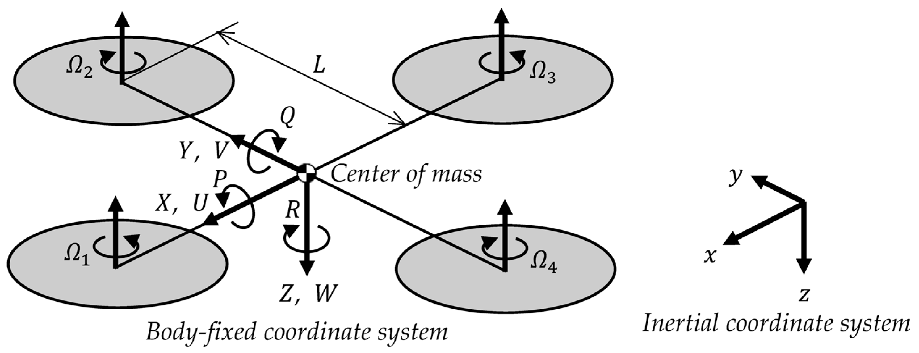
Figure 3 shows the body-fixed coordinate system, state variables, and control inputs used in this study to model the quadrotor. In the body-fixed coordinate system, the translational velocities along the $X$, $Y$, and $Z$ axes are denoted by $U$, $V$, and $W$, respectively, and the angular velocities around these axes by $P$, $Q$, and $R$. The quadrotor is assumed to generate thrust in the direction normal to the $X$-$Y$ plane of the body frame. The angular velocities of the four rotors, which generate this thrust, are denoted by ${\Omega }_1$, ${\Omega }_2$, ${\Omega }_3$, and ${\Omega }_4$. The distance from the quadrotor’s center of mass to where each rotor’s thrust force acts is represented by $L$.

The dynamics of the quadrotor consist of translational and rotational motion and are described by the following equations.

$$\dot{\mathbf{V}}=-\tilde{\mathsf{\Omega }}\mathbf{V}+{\displaystyle \frac{1}{M}}\mathbf{F}$$

(55)

$$\dot{\mathsf{\Omega }}=-{\mathbf{J}}^{-1}\tilde{\mathsf{\Omega }}\mathbf{J}\mathsf{\Omega }+{\mathbf{J}}^{-1}\mathbf{M}$$

(56)

$M$ is the mass of the quadrotor, and $\mathbf{J}$ is the inertia tensor, denoted by

$$\mathbf{J}=\left[\begin{array}{ccc}{J}_{XX}& 0& 0\\ 0& J_{YY}& 0\\ 0& 0& J_{ZZ}\end{array}\right]$$

(57)

In Equations (55) and (56), $\mathbf{V}={\left[\begin{array}{ccc}U& V& W\end{array}\right]}^T$ and $\mathsf{\Omega }={\left[\begin{array}{ccc}P& Q& R\end{array}\right]}^T$ denote the velocity vector and angular velocity vector in the body-fixed coordinate system. $\tilde{\mathsf{\Omega }}$ is the skew-symmetric matrix of angular velocities, defined as

$$\tilde{\mathsf{\Omega }}=\left[\begin{array}{ccc}0& -R& Q\\ R& 0& -P\\ -Q& P& 0\end{array}\right]$$

(58)

The force vector, $\mathbf{F}$, and moment vector, $\mathbf{M}$, act on the quadrotor and can be expressed as

$$\mathbf{F}=\left[\begin{array}{c}{F}_x\\ F_y\\ F_z\end{array}\right]={\mathbf{F}}_p+{\mathbf{F}}_d$$

(59)

$$\mathbf{M}=\left[\begin{array}{c}{M}_x\\ M_y\\ M_z\end{array}\right]={\mathbf{M}}_p+{\mathbf{M}}_d$$

(60)

where ${\mathbf{F}}_p$ and ${\mathbf{M}}_p$ represent the force vector and moment vector generated by the propellers, defined by

$${\mathbf{F}}_p=\left[\begin{array}{c}0\\ 0\\ -C_L\left({\Omega }_1^2+{\Omega }_2^2+{\Omega }_3^2+{\Omega }_4^2\right)\end{array}\right]$$

(61)

$${\mathbf{M}}_p=\left[\begin{array}{c}L{C}_L\left({\Omega }_4^2-{\Omega }_2^2\right)\\ L{C}_L\left({\Omega }_1^2-{\Omega }_3^2\right)\\ C_D\left({\Omega }_1^2-{\Omega }_2^2+{\Omega }_3^2-{\Omega }_4^2\right)\end{array}\right]$$

(62)

Thrust and counter-torque are proportional to the square of the propeller speeds. The constants $C_L$ and $C_D$ depend on the aerodynamic characteristics of the propeller blades, which, in turn, depend on their geometry. Although the quadrotor is subject to gyroscopic moments induced by the rotating propellers, these effects are relatively minor and, therefore, neglected in this study. The second terms, ${\mathbf{F}}_d$ and ${\mathbf{M}}_d$, in Equations (55) and (56) represent external disturbances such as wind gusts.

Let the position of the quadrotor in the inertial frame be defined as $\mathsf{\zeta }={\left[\begin{array}{ccc}x& y& z\end{array}\right]}^{\mathrm{T}}$ and its attitude be represented using Euler angle $\mathsf{\eta }={\left[\begin{array}{ccc}\Phi & \Theta & \Psi \end{array}\right]}^{\mathrm{T}}$. Then, the translational and rotational motion can be rewritten using the velocity vector, $\mathbf{V}$, and the angular velocity vector, $\mathsf{\Omega }$, in the body-fixed coordinate system as

$$\ddot{\mathit{\zeta }}={\dot{\mathbf{R}}}_t\left(\mathsf{\eta },\dot{\mathsf{\eta }}\right)\mathbf{V}+{\mathbf{R}}_t\left(\mathsf{\eta }\right)\dot{\mathbf{V}}$$

(63)

$$\ddot{\mathsf{\eta }}={\dot{\mathbf{R}}}_r\left(\mathsf{\eta },\dot{\mathsf{\eta }}\right)\mathsf{\Omega }+{\mathbf{R}}_r\left(\mathsf{\eta }\right)\dot{\mathsf{\Omega }}$$

(64)

where ${\mathbf{R}}_t\left(\mathsf{\eta }\right)$ and ${\mathbf{R}}_r\left(\mathsf{\eta }\right)$ are the coordinate transformation matrices from the body-fixed coordinate system to the inertial coordinate system, defined as

$${\mathbf{R}}_t\left(\mathsf{\eta }\right)=\left[\begin{array}{ccc}\cos \Psi \cos \Theta & \cos \Psi \sin \Theta \sin \Phi -\sin \Psi \cos \Phi & \cos \Psi \sin \Theta \cos \Phi +\sin \Psi \sin \Phi \\ \sin \Psi \cos \Theta & \sin \Psi \sin \Theta \sin \Phi +\cos \Psi \cos \Phi & \sin \Psi \sin \Theta \cos \Phi -\cos \Psi \sin \Phi \\ -\sin \Theta & \cos \Theta \sin \Phi & \cos \Theta \cos \Phi \end{array}\right]$$

(65)

$${\mathbf{R}}_r\left(\mathsf{\eta }\right)=\left[\begin{array}{ccc}1& \sin \Phi \tan \Theta & \cos \Phi \tan \Theta \\ 0& \cos \Phi & -\sin \Phi \\ 0& \sin \Phi /\cos \Theta & \cos \Phi /\cos \Theta \end{array}\right]$$

(66)

As shown above, the coordinate transformation matrix, ${\mathbf{R}}_r\left(\mathsf{\eta }\right)$, becomes singular at $\Theta =\pm \pi /2$. This singularity can be avoided by using a quaternion representation. However, since this study is limited to normal flight conditions that do not involve acrobatic maneuvers, it is assumed that $\Theta$ remains within the range that avoids the singularity.

Using the above definitions, the equations of motion in the inertial frame can be rewritten as

$$\ddot{\mathsf{\zeta }}=\mathbf{g}+{\dot{\mathbf{R}}}_t\left(\mathsf{\eta },\dot{\mathsf{\eta }}\right)\mathbf{V}-{\mathbf{R}}_t\left(\mathsf{\eta }\right)\tilde{\mathsf{\Omega }}\mathbf{V}+{\mathbf{R}}_t\left(\mathsf{\eta }\right){\displaystyle \frac{1}{M}}\mathbf{F}$$

(67)

$$\ddot{\mathsf{\eta }}={\mathbf{R}}_r\left(\dot{\mathsf{\eta }}\right)\mathsf{\Omega }-{\mathbf{R}}_r\left(\mathsf{\eta }\right){\mathbf{J}}^{-1}\tilde{\mathsf{\Omega }}\mathbf{J}\mathsf{\Omega }+{\mathbf{R}}_r\left(\mathsf{\eta }\right){\mathbf{J}}^{-1}\mathbf{M}$$

(68)

The influence of gravity is considered in the translational equation of motion shown in Equation (67) by adding the gravitational acceleration vector, $\mathbf{g}={\left[\begin{array}{ccc}0& 0& g\end{array}\right]}^{\mathrm{T}}$, as the first term on the right-hand side, where $g$ denotes the gravitational acceleration.

Lastly, assuming that each rotor follows first-order lag dynamics, the propeller angular velocities, ${\Omega }_1$, ${\Omega }_2$, ${\Omega }_3$, and ${\Omega }_4$, follow the propeller commands ${\Omega }_{c1}$, ${\Omega }_{c2}$, ${\Omega }_{c3}$, and ${\Omega }_{c4}$ according to

$$\left[\begin{array}{c}{\dot{\Omega }}_1\\ {\dot{\Omega }}_2\\ {\dot{\Omega }}_3\\ {\dot{\Omega }}_4\end{array}\right]=\left[\begin{array}{c}-{\Omega }_1/T_{\Omega }+{\Omega }_{c1}/T_{\Omega }\\ -{\Omega }_2/T_{\Omega }+{\Omega }_{c2}/T_{\Omega }\\ -{\Omega }_3/T_{\Omega }+{\Omega }_{c3}/T_{\Omega }\\ -{\Omega }_4/T_{\Omega }+{\Omega }_{c4}/T_{\Omega }\end{array}\right]$$

(69)

where $T_{\Omega }$ is the time constant that characterizes the propeller dynamics.

3.2. Linearization of Equations of Motion

As described in Section 2, the proposed RPFC and conventional PFC are designed for linear systems. Therefore, the nonlinear dynamics derived in the previous subsection cannot be directly used. In this subsection, we introduce a method for linearizing the quadrotor dynamics to enable the application of RPFC and PFC. The nonlinear equations of motion, as expressed in Equations (67) and (68), include terms accounting for centripetal acceleration, the product of inertia, and other dynamic effects, making the model complex. In this study, we assume the quadrotor operates near hovering with small deviations in attitude. The following assumptions are made:

Assumption 1: The variations in Euler angles are small, allowing the coordinate transformation matrix, ${\mathbf{R}}_r\left(\mathsf{\eta }\right)$, and the time derivatives of ${\mathbf{R}}_t\left(\mathsf{\eta }\right)$ and ${\mathbf{R}}_r\left(\mathsf{\eta }\right)$ to be approximated as

$${\mathbf{R}}_r\left(\mathsf{\eta }\right)\cong {\mathbf{I}}_3$$

(70)

$${\dot{\mathbf{R}}}_t\left(\mathsf{\eta },\dot{\mathsf{\eta }}\right)={\dot{\mathbf{R}}}_r\left(\mathsf{\eta },\dot{\mathsf{\eta }}\right)\cong {\mathbf{0}}_3$$

(71)

where ${\mathbf{0}}_3$ and ${\mathbf{I}}_3$ denote the $3\times 3$ zero and identity matrices, respectively.

Assumption 2: The effects of centripetal acceleration are negligible:

$$\tilde{\mathsf{\Omega }}\mathbf{V}\cong \left[\begin{array}{c}0\\ 0\\ 0\end{array}\right]$$

(72)

Assumption 3: The effects of the inertial cross-coupling are negligible:

$$\tilde{\mathsf{\Omega }}\mathbf{J}\mathsf{\Omega }\cong \left[\begin{array}{c}0\\ 0\\ 0\end{array}\right]$$

(73)

Using these assumptions, we linearize Equations (67) and (68). First, we define a new input vector, $\mathbf{f}$, as the transformation of the force vector, $\mathbf{F}$, in the body-fixed coordinate system into the inertial coordinate system.

$$\mathbf{f}=\left[\begin{array}{c}{f}_x\\ f_y\\ f_z\end{array}\right]={\mathbf{R}}_t\left(\mathsf{\eta }\right)\mathbf{F}$$

(74)

Thus, $\mathbf{f}$ represents the force vector in the inertial coordinate system. Applying Assumptions 1 and 2 shown in Equations (71) and (72), the translational dynamics become

$$\ddot{\mathsf{\zeta }}=\mathbf{g}+{\displaystyle \frac{1}{M}}\mathbf{f}$$

(75)

We then define a new control input, ${\mathbf{f}}_u$, by

$$\mathbf{f}={\mathbf{f}}_u-M\mathbf{g}$$

(76)

In this equation, ${\mathbf{f}}_u$ is the control input determined by the controller, while $M\mathbf{g}$ is the constant input that cancels out the effect of gravity. Substituting this input, $\mathbf{f}$, into the equation obtains

$$\ddot{\mathsf{\zeta }}={\displaystyle \frac{1}{M}}{\mathbf{f}}_u$$

(77)

Letting the state vector for translational motion be ${\mathbf{x}}_t={\left[\begin{array}{cc}{\mathsf{\zeta }}^{\mathrm{T}}& {\dot{\mathsf{\zeta }}}^{\mathrm{T}}\end{array}\right]}^{\mathrm{T}}$ and the output be ${\mathbf{y}}_t=\mathsf{\zeta }$, we can represent the system in state-space

$${\displaystyle \frac{d{\mathbf{x}}_t}{dt}}=\left[\begin{array}{cc}{\mathbf{0}}_3& {\mathbf{I}}_3\\ {\mathbf{0}}_3& {\mathbf{0}}_3\end{array}\right]{\mathbf{x}}_t+\left[\begin{array}{c}{\mathbf{0}}_3\\ \left(1/M\right){\mathbf{I}}_3\end{array}\right]{\mathbf{f}}_u$$

(78)

$${\mathbf{y}}_t=\left[\begin{array}{cc}{\mathbf{I}}_3& {\mathbf{0}}_3\end{array}\right]{\mathbf{x}}_t$$

(79)

Consequently, the system is square and linear, with a six-dimensional state vector, three inputs, and three outputs, which enables the application of both PFC and RPFC.

Next, we linearize the rotational dynamics expressed in Equation (68). By applying Assumptions 1 and 3 shown in Equations (70), (71) and (73), the rotational dynamics can be simplified to

$$\ddot{\mathsf{\eta }}={\mathbf{J}}^{-1}\mathbf{M}$$

(80)

Letting the state vector for rotational motion be ${\mathbf{x}}_r={\left[\begin{array}{cc}{\mathsf{\eta }}^{\mathrm{T}}& {\dot{\mathsf{\eta }}}^{\mathrm{T}}\end{array}\right]}^{\mathrm{T}}$ and the output be ${\mathbf{y}}_r=\mathsf{\eta }$, the corresponding state-space representation becomes

$${\displaystyle \frac{d{\mathbf{x}}_r}{dt}}=\left[\begin{array}{cc}{\mathbf{0}}_3& {\mathbf{I}}_3\\ {\mathbf{0}}_3& {\mathbf{0}}_3\end{array}\right]{\mathbf{x}}_r+\left[\begin{array}{c}{\mathbf{0}}_3\\ {\mathbf{J}}^{-1}\end{array}\right]\mathbf{M}$$

(81)

$${\mathbf{y}}_r=\left[\begin{array}{cc}{\mathbf{I}}_3& {\mathbf{0}}_3\end{array}\right]{\mathbf{x}}_r$$

(82)

As in the linearized translational case, the linearized rotational dynamics is square and linear, with a six-dimensional state vector, three inputs, and three outputs, which enables the application of both PFC and RPFC.

Finally, since the linearized translational and rotational equations of motion described above represent continuous-time systems, discretization is required to apply PFC and RPFC. In this study, the systems provided in Equations (78) and (81) were discretized using a zero-order hold (ZOH) method [34], assuming that the control inputs remain constant over each sampling time, $∆t$.

3.3. Flight Control System of the Quadrotor

The RPFC and PFC determine the translational control input, ${\mathbf{f}}_u$, and the rotational control input, $\mathbf{M}$, using the discretized version of the linearized motion models described in Equations (78) and (81). The translational controller receives the position command ${\mathsf{\zeta }}_c={\left[\begin{array}{ccc}{x}_c& y_c& z_c\end{array}\right]}^T$ in the inertial coordinate system and generates input ${\mathbf{f}}_u$, which guides the quadrotor to the desired position. It is important to note that input ${\mathbf{f}}_u$ in the linearized translational motion equation represents force in the inertial coordinate system. Since the direction of thrust for a quadrotor is fixed along the body’s vertical axis, the generated force cannot be directly applied in horizontal directions when the quadrotor is hovering. Thus, to produce a horizontal force, the quadrotor must change its attitude to tilt the thrust direction. In this way, the quadrotor generates the required force for horizontal movement and achieves the desired flight control.

The total thrust, $F_z$, of the quadrotor is determined as the Euclidean norm of the force vector, $\mathbf{f}$, in the inertial frame:

$$F_z=-{‖\mathbf{f}‖}_2=\sqrt{f_x^2+f_y^2+f_z^2}$$

(83)

Assuming that the yaw angle, $\Psi$, is controlled to be 0 degrees ($\Psi =0$), the relationship between the total thrust, $F_z$, and the inertial input, $\mathbf{f}$, can be expressed using the coordinate transformation matrix ${\mathbf{R}}_r\left(\mathsf{\eta }\right)$ as

$$\left[\begin{array}{c}\sin \Theta \cos \Phi \\ -\sin \Phi \\ \cos \Theta \cos \Phi \end{array}\right]F_z=\left[\begin{array}{c}{f}_x\\ f_y\\ f_z\end{array}\right]$$

(84)

The commanded roll, ${\Phi }_c$, and pitch, ${\Theta }_c$, angles for the rotational controller are then derived as follows:

$${\Phi }_c={\sin }^{-1}\left(-f_y/F_z\right)$$

(85)

$${\Theta }_c={\tan }^{-1}\left(f_x/f_z\right)$$

(86)

Since the yaw angle, $\Psi$, is assumed to be 0 degrees, the commanded yaw angle, ${\Psi }_c$, is also set to 0 degrees. The commanded attitude, ${\mathsf{\eta }}_c$, in Euler angles is expressed as

$${\mathsf{\eta }}_c=\left[\begin{array}{c}{\Phi }_c\\ {\Theta }_c\\ {\Psi }_c\end{array}\right]=\left[\begin{array}{c}{\Phi }_c\\ {\Theta }_c\\ 0\end{array}\right]$$

(87)

Figure 4 is a block diagram of the proposed flight control system for the quadrotor. In the proposed flight control system, the translational controller determines the control input, ${\mathbf{f}}_u$, in the inertial coordinate system. Then, the Euler angle command generator calculates the attitude command by considering both the gravity-compensated input, $\mathbf{f}$, and the total thrust, $F_z$. The rotational controller then tracks the commanded attitude angles, ${\mathsf{\eta }}_c$, to ensure the quadrotor follows the desired orientation.

Finally, in the input mixing block shown in Figure 4, the angular velocity commands of the propellers, ${\Omega }_{c1}$, ${\Omega }_{c2}$, ${\Omega }_{c3}$, and ${\Omega }_{c4}$, are determined using the total thrust, $F_z$, provided by the translational controller and the control moment, $\mathbf{M}$, provided by the rotational controller, according to the following equation:

$${\Omega }_{c1}^2=-{\displaystyle \frac{F_z}{4C_L}}+{\displaystyle \frac{M_y}{2L{C}_L}}+{\displaystyle \frac{M_z}{4C_D}}$$

(88)

$${\Omega }_{c2}^2=-{\displaystyle \frac{F_z}{4C_L}}-{\displaystyle \frac{M_x}{2L{C}_L}}-{\displaystyle \frac{M_z}{4C_D}}$$

(89)

$${\Omega }_{c3}^2=-{\displaystyle \frac{F_z}{4C_L}}-{\displaystyle \frac{M_y}{2L{C}_L}}+{\displaystyle \frac{M_z}{4C_D}}$$

(90)

$${\Omega }_{c4}^2=-{\displaystyle \frac{F_z}{4C_L}}+{\displaystyle \frac{M_x}{2L{C}_L}}-{\displaystyle \frac{M_z}{4C_D}}$$

(91)

4. Numerical Simulation

In this section, the control performance of the proposed RPFC is evaluated and compared with that of conventional PFC using the quadrotor flight control system described in Section 3. The proposed flight controller consists of two components, namely, the translational controller and the rotational controller. The comparison is conducted by applying either RPFC or PFC to both components of the system. It is also assumed that all state variables are fully observable.

Table 1. The parameters of the quadrotor and the simulation settings.

Physical Significance	Symbol	Value
Mass of quadrotor $\left[\mathrm{k}\mathrm{g}\right]$	$M$	$0.5$
Distance from the center of mass to each rotor $\left[\mathrm{m}\right]$	$L$	$0.2$
Moments of inertia $\left[\mathrm{k}\mathrm{g}{\mathrm{m}}^2\right]$	$\left[\begin{array}{ccc}{J}_{XX}& J_{YY}& J_{ZZ}\end{array}\right]$	$\left[\begin{array}{ccc}0.008& 0.009& 0.015\end{array}\right]$
Lift coefficient of the propellers	$C_L$	$5.0\times {10}^{-6}$
Drag coefficient of the propellers	$C_D$	$5.0\times {10}^{-7}$
Time constant of the propellers $\left[\mathrm{s}\right]$	$T_{\Omega }$	$0.02$
Sampling time $\left[\mathrm{s}\right]$	$∆t$	$0.01$
Simulation time $\left[\mathrm{s}\right]$	$T_{end}$	$100$
Sample size	$n_k$	$\mathrm{10,001}$
Amplitudes of the target position $\left[\mathrm{m}\right]$	$\left[\begin{array}{ccc}{c}_x& c_y& c_z\end{array}\right]$	$\left[\begin{array}{ccc}2.5& 2.5& -2\end{array}\right]$
Angular frequency of the target position $\left[\mathrm{r}\mathrm{a}\mathrm{d}/\mathrm{s}\right]$	${\omega }_c$	$2\pi /T_{end}$
Magnitudes of the disturbances $\left[\mathrm{N}\right]$	$\left[\begin{array}{ccc}{d}_x& d_y& d_z\end{array}\right]$	$\left[\begin{array}{ccc}0.5& -0.5& 0.5\end{array}\right]$
Magnitudes of the disturbances $\left[\mathrm{N}\mathrm{m}\right]$	$\left[\begin{array}{ccc}{d}_P& d_Q& d_R\end{array}\right]$	$\left[\begin{array}{ccc}0.07& 0.07& -0.07\end{array}\right]$
Angular frequency of the disturbance $\left[\mathrm{r}\mathrm{a}\mathrm{d}/\mathrm{s}\right]$	${\omega }_d$	$2\pi /3$

details the simulation settings, including the quadrotor parameters.

Table 2. The parameters for the translational controller.

Physical Significance	Symbol	Value
Coincidence point for output	$\left[\begin{array}{ccc}{i}_1& i_2& i_3\end{array}\right]$	$\left[\begin{array}{ccc}80& 90& 150\end{array}\right]$
Coincidence point for switching function	$\left[\begin{array}{ccc}{i}_{\sigma 1}& i_{\sigma 2}& i_{\sigma 3}\end{array}\right]$	$\left[\begin{array}{ccc}100& 110& 200\end{array}\right]$
Time constant of the reference trajectory $\left[\mathrm{s}\right]$	$T$	$0.2$
Time constant of the reference trajectory $\left[\mathrm{s}\right]$	$T_{\sigma }$	$0.5$
Coefficient matrix of the hypersurface	$\mathbf{S}$	$\left[\begin{array}{cc}{\mathbf{I}}_3& 10{\mathbf{I}}_3\end{array}\right]$

and

Table 3. The parameters for the rotational controller.

Physical Significance	Symbol	Value
Coincidence point for output	$\left[\begin{array}{ccc}{i}_1& i_2& i_3\end{array}\right]$	$\left[\begin{array}{ccc}15& 20& 100\end{array}\right]$
Coincidence point for switching function	$\left[\begin{array}{ccc}{i}_{\sigma 1}& i_{\sigma 2}& i_{\sigma 3}\end{array}\right]$	$\left[\begin{array}{ccc}15& 20& 100\end{array}\right]$
Time constant of the reference trajectory $\left[\mathrm{s}\right]$	$T$	$0.05$
Time constant of the reference trajectory $\left[\mathrm{s}\right]$	$T_{\sigma }$	$0.2$
Coefficient matrix of the hypersurface	$\mathbf{S}$	$\left[\begin{array}{cc}{\mathbf{I}}_3& 10{\mathbf{I}}_3\end{array}\right]$

list the parameters used for the translational and rotational controllers, respectively. As discussed in Section 3, a key feature of the proposed flight control system is that attitude control is directly achieved via propeller thrusts in the rotational controller, while translational control is indirectly realized by tilting the attitude to generate forces in the translational directions. Therefore, the translational controller’s performance depends on the responsiveness of the rotational controller, and a slower response in the translational controller is preferred. Accordingly, the time constants, $T$ and $T_{\sigma },$ of the reference trajectories in Equations (18) and (45) are set such that the translational controller’s time constant is greater than that of the rotational controller.

Next, the position command, ${\mathsf{\zeta }}_c\left(k\right)$, for the translational controller is provided by the following equation.

$${\mathsf{\zeta }}_c\left(k\right)=\left[\begin{array}{c}{c}_x\sin \left({\omega }_{c}k∆t\right)\\ -c_y\cos \left({\omega }_{c}k∆t\right)\\ c_z\end{array}\right]$$

(92)

Additionally, external force disturbances, ${\mathbf{F}}_d$, and moment disturbances, ${\mathbf{M}}_d$, are applied under three conditions, as shown in

Table 4. The disturbance conditions in the simulation.

Condition	Disturbance ${\mathbf{F}}_{\mathit{d}}$	Disturbance ${\mathbf{M}}_{\mathit{d}}$
1	${\mathbf{F}}_d={\left[\begin{array}{ccc}0& 0& 0\end{array}\right]}^{\mathrm{T}}$	${\mathbf{M}}_d={\left[\begin{array}{ccc}0& 0& 0\end{array}\right]}^{\mathrm{T}}$
2	${\mathbf{F}}_d={\left[\begin{array}{ccc}{d}_x& d_y& d_z\end{array}\right]}^{\mathrm{T}}$	${\mathbf{M}}_d={\left[\begin{array}{ccc}{d}_P& d_Q& d_R\end{array}\right]}^{\mathrm{T}}$
3	${\mathbf{F}}_d\left(t\right)={\left[\begin{array}{ccc}{d}_x& d_y& d_z\end{array}\right]}^{\mathrm{T}}\cos \left({\omega }_{d}k∆t\right)$	${\mathbf{M}}_d\left(t\right)={\left[\begin{array}{ccc}{d}_P& d_Q& d_R\end{array}\right]}^{\mathrm{T}}\sin \left({\omega }_{d}k∆t\right)$

. Condition 1 assumes a nominal state without disturbances; Condition 2 introduces constant disturbances, which are intended to represent parameter uncertainties such as mass and moments of inertia, or steady wind forces; and Condition 3 considers periodically varying disturbances, representing external forces caused by events such as gusts of wind. Under these three conditions, where the position command, ${\mathsf{\zeta }}_c$; force disturbance, ${\mathbf{F}}_d$; and moment disturbance, ${\mathbf{M}}_d$, are applied, the performance of flight control systems using RPFC and PFC is evaluated.

In this study, quantitative metrics are used to evaluate both the tracking performance and the magnitude of the control input. First, the tracking performance is assessed using the Integral of Squared Error (ISE), which is defined as follows:

$$ise=\sum _{k=0}^{n_k-1}{e}_l^2$$

(93)

where $e_l$ ($l=x$, $y$, $z$, $\Phi$, $\Theta$, $\Psi$) denotes the tracking error for each output variable.

Next, the control input is evaluated using the mean squared value (MSV) of the propeller rotational speeds, defined as

$$msv={\displaystyle \frac{1}{n_k}}\sum _{k=0}^{n_k-1}{\Omega }_l^2$$

(94)

where ${\Omega }_l$ ($l=1$, $2$, $3$, $4$) denotes the rotational speed of each propeller.

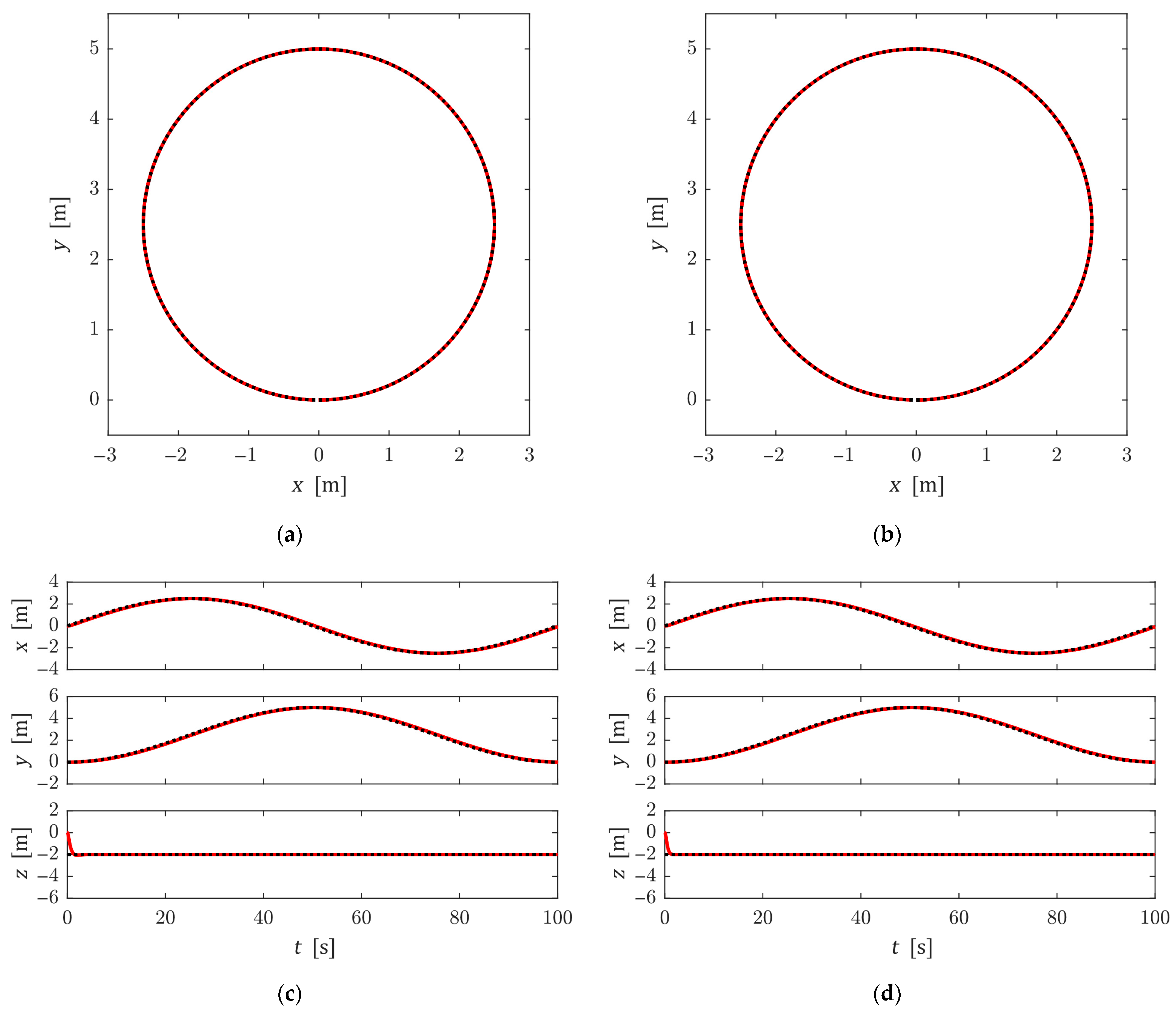
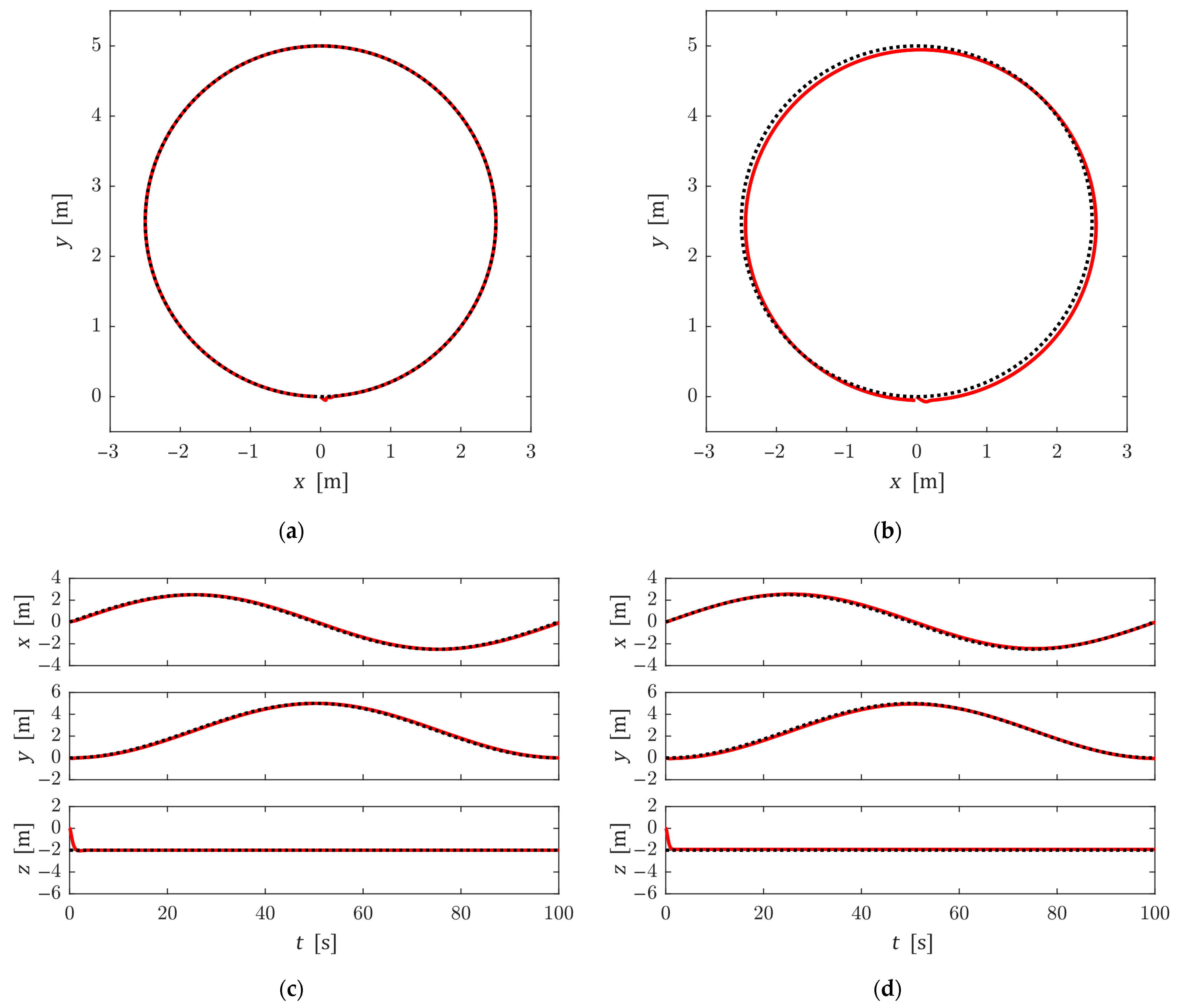
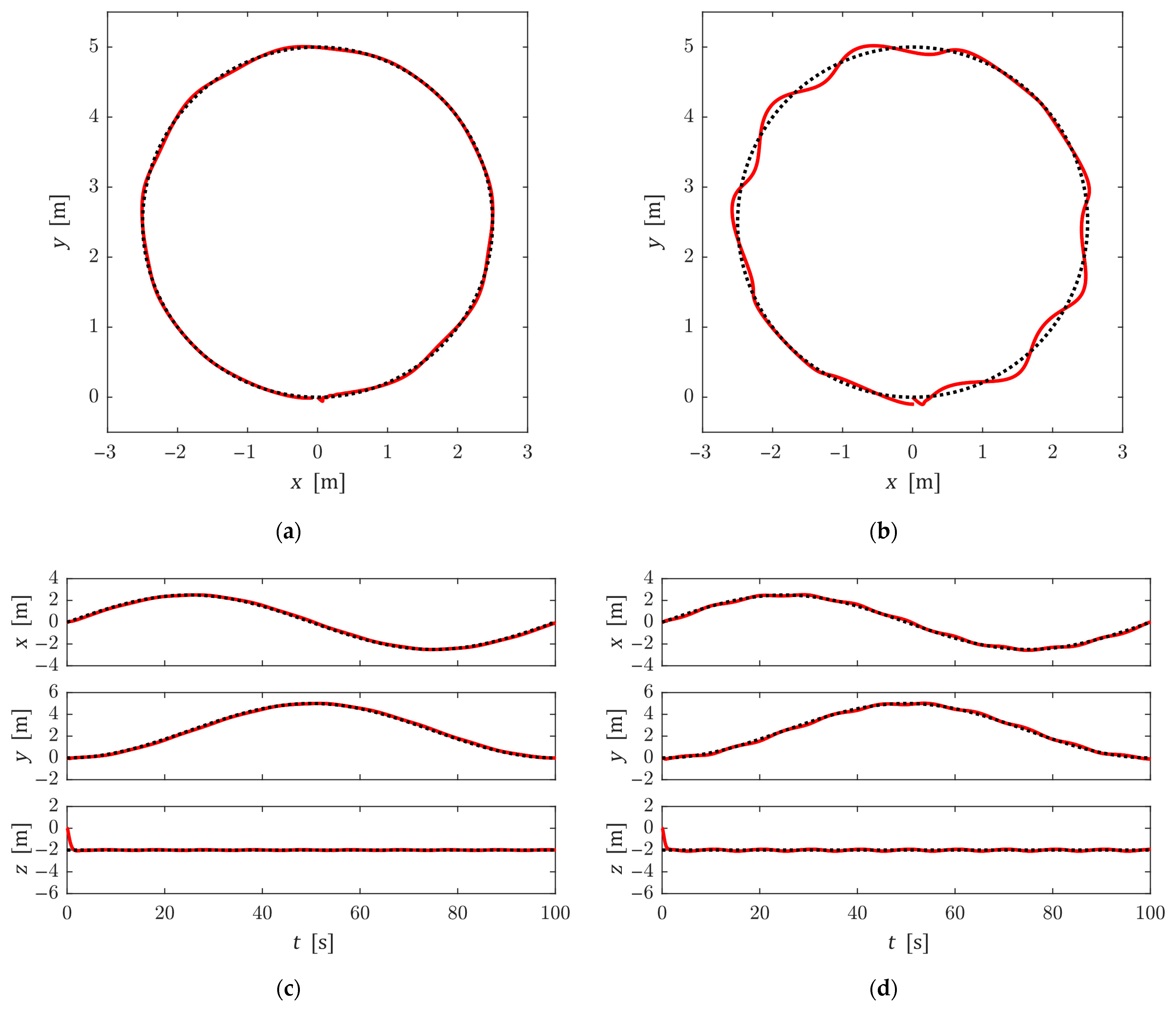
Figure 5, Figure 6 and Figure 7 show the time responses of the position and attitude of the quadrotor under Conditions 1 to 3. In these figures, the black dashed lines represent the command values for both translational and rotational controllers, while the red solid lines denote the output responses. The initial state of the quadrotor is assumed to be a hovering condition with an initial position of $\mathsf{\zeta }\left(0\right)={\left[\begin{array}{ccc}0& 0& 0\end{array}\right]}^{\mathrm{T}}$ and an initial attitude of $\mathsf{\eta }\left(0\right)={\left[\begin{array}{ccc}0& 0& 0\end{array}\right]}^{\mathrm{T}}$.

In Condition 1 (Figure 5), where no disturbances are applied, both PFC and the proposed RPFC successfully track the position commands. Attitude commands generated by the translational controller are also well tracked. Although the ISE values shown in

Table 5. ISE values of the position and the Euler angle in each controller.

Condition	Output	RPFC	Difference (vs. PFC)	PFC
1	$x$	33.080	+2.747%	32.195
	$y$	33.276	+2.445%	32.482
	$z$	149.206	+6.991%	139.457
	$\Phi$	0.000	0.000%	0.000
	$\Theta$	0.051	+65.273%	0.031
	$\Psi$	0.000	0.000%	0.000
2	$x$	32.633	−50.616%	66.080
	$y$	33.429	−45.906%	61.798
	$z$	152.078	−23.536%	198.890
	$\Phi$	0.635	−96.716%	19.341
	$\Theta$	0.449	−97.058%	15.249
	$\Psi$	0.001	−99.973%	5.464
3	$x$	35.078	−52.805%	74.326
	$y$	35.746	−53.222%	76.418
	$z$	154.495	−14.351%	180.381
	$\Phi$	1.372	−90.201%	14.001
	$\Theta$	1.066	−90.638%	11.391
	$\Psi$	0.008	−99.718%	2.732

indicate a slightly higher value for RPFC in relative terms, the absolute differences are small, and no significant performance gap can be observed between the controllers.

Condition 2 (Figure 6) includes constant disturbances, and the PFC shows degradation in position tracking performance compared with the nominal case. The rotational controller also exhibits steady-state errors in attitude tracking. By contrast, the proposed RPFC demonstrates robust tracking performance, maintaining almost the same performance as in the nominal case. This is also supported by the ISE values in Table 5, which show that RPFC achieves lower ISE values than PFC, indicating improved performance under constant disturbances.

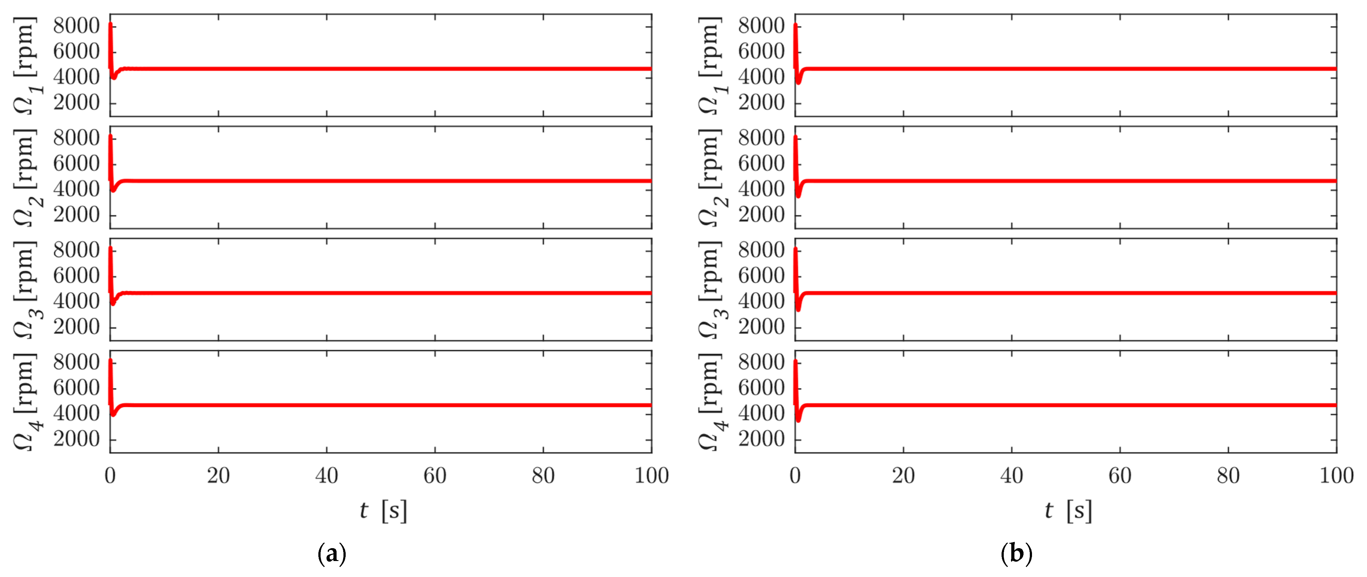
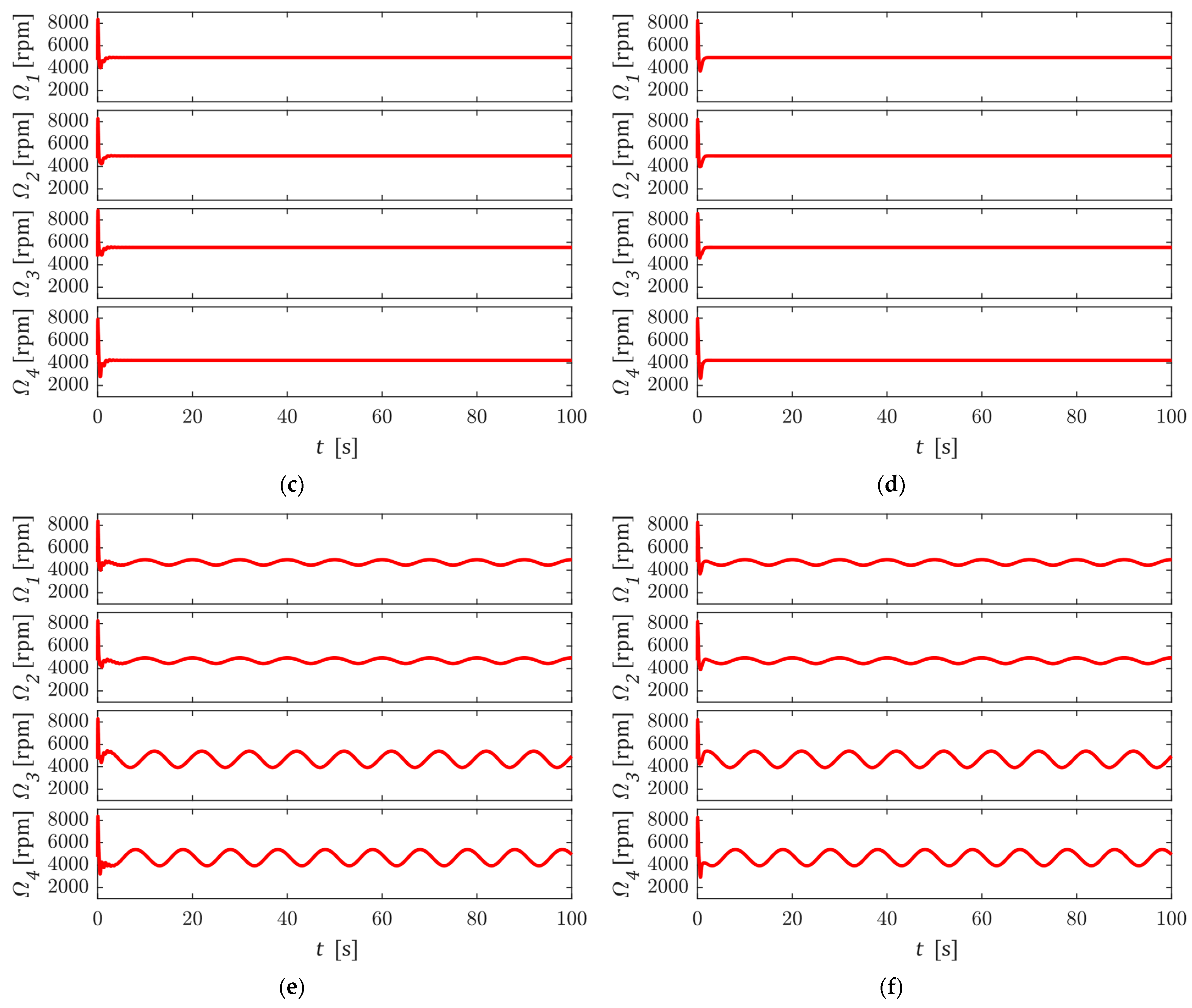
Condition 3 (Figure 7) includes periodic disturbances, and PFC fails to track the reference trajectories accurately. Although RPFC is also affected by the disturbances, it maintains a trajectory closer to the reference. The ISE values confirm that RPFC consistently outperforms PFC under all outputs, indicating its superior performance under periodic disturbances. Figure 8 illustrates the time history of the rotor speeds. It shows that RPFC achieves effective control without significantly increasing control effort compared with PFC. The MSV of the propeller speeds shown in

Table 6. Mean squared values of the propeller speed in each controller.

Condition	Input	RPFC	Difference (vs. PFC)	PFC
1	${\Omega }_1$	245,167	0.0000%	245,167
	${\Omega }_2$	245,167	0.0000%	245,167
	${\Omega }_3$	245,167	0.0000%	245,167
	${\Omega }_4$	245,167	0.0000%	245,167
2	${\Omega }_1$	267,610	+0.0035%	267,601
	${\Omega }_2$	267,607	+0.0026%	267,600
	${\Omega }_3$	337,607	+0.0022%	337,599
	${\Omega }_4$	197,604	+0.0030%	197,598
3	${\Omega }_1$	243,909	+0.0064%	243,893
	${\Omega }_2$	243,901	+0.0046%	243,890
	${\Omega }_3$	243,903	+0.0057%	243,890
	${\Omega }_4$	243,897	+0.0040%	243,887

also indicates no noticeable difference under nominal conditions (Condition 1). A slight increase in input magnitude is observed only under disturbed conditions (Conditions 2 and 3), confirming that the proposed controller effectively suppresses the influence of disturbances.

These results verify that the proposed RPFC achieves higher robustness than conventional PFC in quadrotor flight control systems. However, the ISE (Integral of Squared Error) values also indicate that the increase in error under disturbances is larger in the translational control system than in the rotational control system. The linearized model used for controller design in this study features an equal number of inputs and degrees of freedom, which ensures that the matching conditions are satisfied even under parameter variations and external forces such as wind gusts. In practice, however, actuator delays exist and make it difficult to fully meet this condition.

Focusing on how control inputs are generated, rotational motion is directly driven by changing the propeller speeds, which produce torque directly. Since the propeller response is significantly faster than the overall system dynamics, the effect of actuator delays is relatively small. On the other hand, translational motion is indirectly controlled by tilting the body to change the direction of the thrust vector. Therefore, the control input applied to the translational control system can only be regarded as pseudo-fully actuated. This difference in input mechanism is the reason why the rotational controller demonstrated better performance than the translational controller under disturbance conditions.

5. Conclusions

This study proposed a novel Robust Predictive Function Control (RPFC) method aimed at improving the robustness of conventional Predictive Function Control (PFC). The proposed RPFC and the conventional PFC were implemented in a quadrotor flight control system, and their performance was verified under constant and periodically varying disturbance conditions through numerical simulations. The results demonstrated that RPFC achieves superior control performance compared with PFC in the presence of disturbances. Future work will focus on applying the proposed controller to an actual quadrotor and validating its effectiveness through flight experiments.

References

1. Maciejowski, J.M. Predictive Control: With Constraints; Prentice Hall Press: Hoboken, NJ, USA, 2000. [Google Scholar]
2. Morari, M.; Lee, J.H. Model Predictive Control: Past, Present and Future. J. Comput. Appl. Chem. Eng. 1999, 23, 667–682. [Google Scholar] [CrossRef]
3. Qin, S.J.; Badgwell, T.A. A Survey of Industrial Model Predictive Control Technology. IFAC Control. Eng. Pract. 2003, 11, 733–764. [Google Scholar] [CrossRef]
4. Nguyen, H.; Kamel, M.; Alexis, K.; Siegwart, R. Model Predictive Control for Micro Aerial Vehicles: A Survey. In Proceedings of the European Control Conference (ECC), Delft, The Netherlands, 29 June–2 July 2021; pp. 1556–1563. [Google Scholar] [CrossRef]
5. Eren, U.; Prach, A.; Kocer, B.B.; Rakovic, S.V.; Kayacan, E.; Acikmese, B. Model Predictive Control in Aerospace Systems: Current State and Opportunities. AIAA J. Guid. Control. Dyn. 2017, 40, 1541–1566. [Google Scholar] [CrossRef]
6. Oh, D.D.; Byun, J.; Lee, D. Real-Time Trajectory Generation of a Quadrotor UAV with Load Suspended from a Pulley. In Proceedings of the International Conference on Control, Automation and Systems (ICCAS), Jeju, Republic of Korea, 27 November–1 December 2022; pp. 1309–1314. [Google Scholar] [CrossRef]
7. Islam, M.; Idres, M.M. Dynamics and Control of Quadcopter Using Linear Model Predictive Control Approach. IOP Conf. Ser. Mater. Sci. Eng. 2017, 270, 012007. [Google Scholar] [CrossRef]
8. Koo, S.; Kim, S.; Suk, J. Model Predictive Control for UAV Automatic Landing on Moving Carrier Deck with Heave Motion. IFAC-PapersOnLine 2015, 48, 59–64. [Google Scholar] [CrossRef]
9. Romero, A.; Sun, S.; Foehn, P.; Scaramuzza, D. Model Predictive Contouring Control for Time-Optimal Quadrotor Flight. IEEE Trans. Robot. 2022, 38, 3340–3356. [Google Scholar] [CrossRef]
10. Mao, S.; Tan, W.K.; Low, K.H. Autonomous Formation Flight of Indoor UAVs Based on Model Predictive Control. In Proceedings of the AIAA Science and Technology (SciTech) Forum, San Diego, CA, USA, 3–7 January 2016; p. 0515. [Google Scholar] [CrossRef]
11. Richalet, J.; Ata-Doss, S.E.; Arber, C.; Kuntze, H.; Jacubasch, A.; Schill, W. Predictive Functional Control-Application to Fast and Accurate Robots. IFAC Proc. Vol. 1987, 20, 251–258. [Google Scholar] [CrossRef]
12. Richalet, J.; O’Donovan, D. Predictive Functional Control: Principles and Industrial Applications, 2009th ed.; Springer: Berlin, Germany, 2009. [Google Scholar]
13. Vivas, A.; Poignet, P. Model Based Predictive Control of a Fully Parallel Robot. In Proceedings of the 7th IFAC Symposium on Robot Control, Wroclaw, Poland, 1–3 September 2003; pp. 279–284. [Google Scholar] [CrossRef]
14. Hashimoto, Y.; Satoh, T.; Nagase, J.; Saga, N. Comparison between PFC and PID Control Systems for a Pneumatic Cylinder. IEEJ Trans. Electr. Electron. Eng. 2015, 10, 605–607. [Google Scholar] [CrossRef]
15. Nagase, J.; Satoh, T.; Saga, N.; Suzumori, K. Predictive Functional Control of Tendon-Driven Actuator Using Pneumatic Balloon. J. Adv. Mech. Des. Syst. Manuf. 2013, 7, 752–762. [Google Scholar] [CrossRef]
16. Satoh, T.; Kaneko, K.; Saito, N. Performance Improvement of Predictive Functional Control: A Disturbance Observer Approach. In Proceedings of the 37th Annual Conference of the IEEE Industrial Electronics Society, Victoria, Australia, 7–10 November 2011; pp. 279–284. [Google Scholar] [CrossRef]
17. Hara, H.; Satoh, T.; Saito, N.; Nagase, J.; Saga, N. Disturbance Observer-Based Predictive Functional Control Using Zero Phase Error Tracking Controller. In Proceedings of the World Congress on Industrial Control Systems Security, London, UK, 14–16 December 2015; pp. 19–20. [Google Scholar] [CrossRef]
18. Zhang, Y.; Yang, H.; Jiang, Z.; Hu, F.; Zhang, W. Robust Predictive Functional Control for Flight Vehicles Based on Nonlinear Disturbance Observer. Int. J. Aerosp. Eng. 2015, 2015, 1–16. [Google Scholar] [CrossRef]
19. Utkin, V.I. Sliding Mode Control in Mechanical Systems. In Proceedings of the Annual Conference of IEEE Industrial Electronics, Bologna, Italy, 5–9 September 1994; pp. 1429–1431. [Google Scholar] [CrossRef]
20. Utkin, V.I. Sliding Modes in Control and Optimization, 1st ed.; Springer: Berlin, Germany, 1992; pp. 1–73. [Google Scholar]
21. Utkin, V.I. Integral Sliding Mode in Systems Operating under Uncertainty Conditions. In Proceedings of the IEEE Conference on Decision and Control (CDC), Kobe, Japan, 11–13 December 1996; pp. 4591–4596. [Google Scholar] [CrossRef]
22. Rubagotti, M.; Estrada, A.; Castanos, F.; Ferrara, A.; Fridman, L. Integral Sliding Mode Control for Nonlinear Systems With Matched and Unmatched Perturbations. IEEE Trans. Autom. Control. 2011, 56, 2699–2704. [Google Scholar] [CrossRef]
23. Pan, Y.; Yang, C.; Pan, L.; Yu, H. Integral Sliding Mode Control: Performance, Modification, and Improvement. IEEE Trans. Ind. Inform. 2018, 14, 3087–3096. [Google Scholar] [CrossRef]
24. Woodham, C.A.; Zinober, A.S.I. Eigenvalue Placement in a Specified Sector for Variable Structure Control Systems. Int. J. Control. 1993, 57, 1021–1037. [Google Scholar] [CrossRef]
25. Castillo, I.; Fridman, L. MATLAB Toolbox for Singular LQ Based Sliding Mode Control Design. In Proceedings of the IEEE Conference on Decision and Control, Firenze, Italy, 10–13 December 2013; pp. 4242–4247. [Google Scholar] [CrossRef]
26. Bhattacharjee, D.; Subbarao, K. Robust Control Strategy for Quadcopters using Sliding Mode Control and Model Predictive Control. In Proceedings of the AIAA Science and Technology (SciTech) Forum, Orlando, FL, USA, 6–10 January 2020; pp. 2020–2071. [Google Scholar] [CrossRef]
27. Rubagotti, M.; Raimondo, D.M.; Ferrara, A.; Magni, L. Robust Model Predictive Control With Integral Sliding Mode in Continuous-Time Sampled-Data Nonlinear Systems. IEEE Trans. Autom. Control. 2011, 56, 556–570. [Google Scholar] [CrossRef]
28. Xiao, H.; Zhao, D.; Gao, S.; Spurgeon, S.K. Sliding Mode Predictive Control: A Survey. Annu. Rev. Control. 2022, 54, 148–166. [Google Scholar] [CrossRef]
29. Wang, Y.; Chen, W.; Tomizuka, M.; Alsuwaidan, B.N. Model Predictive Sliding Mode Control: For Constraint Satisfaction and Robustness. In Proceedings of the Dynamic Systems and Control Conference, Palo Alto, CA, USA, 21–23 October 2013. [Google Scholar] [CrossRef]
30. Zhou, J.; Liu, Z.; Pei, R. Sliding Mode Model Predictive Control with Terminal Constraints. In Proceedings of the 3rd World Congress on Intelligent Control and Automation, Hefei, China, 26 June–2 July 2000; pp. 2791–2795. [Google Scholar] [CrossRef]
31. Masuda, K.; Uchiyama, K. Extended Model Predictive Control: Robust Controller with Matching Condition. Trans. JSME 2020, 86, 19-00300. (In Japanese) [Google Scholar] [CrossRef]
32. Masuda, K.; Uchiyama, K. Control System Design by using Extended Model Predictive Control for The Quadrotor. In Proceedings of the AIAA Science and Technology (SciTech) Forum, San Diego, CA, USA, 3–7 January 2022; p. 2022-0753. [Google Scholar] [CrossRef]
33. Masuda, K.; Uchiyama, K. Attitude Control System for Quadrotor Using Robust Monte Carlo Model Predictive Control. Actuators 2024, 13, 443. [Google Scholar] [CrossRef]
34. Franklin, G.F.; Powell, J.D.; Workman, M.L. Digital Control of Dynamic Systems, 3rd ed.; Prentice Hall Press: Hoboken, NJ, USA, 1997. [Google Scholar]
Figure 1. Block diagram of Predictive Functional Controller.
Drones 09 00506 g001
Figure 2. Block diagram of Robust Predictive Functional Controller.
Drones 09 00506 g002
Figure 3. Coordinate definition of the quadrotor.
Drones 09 00506 g003
Figure 4. Block diagram of the proposed flight control system of the quadrotor.
Drones 09 00506 g004
Figure 5. Time histories of the position and attitude of the quadrotor in Condition 1 (black dotted line: command value; red solid line: output). (a) RPFC (trajectory). (b) PFC (trajectory). (c) RPFC (position). (d) PFC (position). (e) RPFC (attitude). (f) PFC (attitude).
Drones 09 00506 g005aDrones 09 00506 g005b
Figure 6. Time histories of the position and the attitude of the quadrotor in Condition 2 (black dotted line: command value; red solid line: output). (a) RPFC (trajectory). (b) PFC (trajectory). (c) RPFC (position). (d) PFC (position). (e) RPFC (attitude). (f) PFC (attitude).
Drones 09 00506 g006aDrones 09 00506 g006b
Figure 7. Time histories of the position and the attitude of the quadrotor in Condition 3 (black dotted line: command value; red solid line: output). (a) RPFC (trajectory). (b) PFC (trajectory). (c) RPFC (position). (d) PFC (position). (e) RPFC (attitude). (f) PFC (attitude).
Drones 09 00506 g007aDrones 09 00506 g007b
Figure 8. Time histories of the rotational speed of the propellers. (a) RPFC (Condition 1). (b) PFC (Condition 1). (c) RPFC (Condition 2). (d) PFC (Condition 2). (e) RPFC (Condition 3). (f) PFC (Condition 3).
Drones 09 00506 g008aDrones 09 00506 g008b