Bounded-Gain Prescribed-Time Robust Spatiotemporal Cooperative Guidance Law for UAVs Under Jointly Strongly Connected Topologies

Abstract

This paper presents a three-dimensional robust spatiotemporal cooperative guidance law for unmanned aerial vehicles (UAVs) to track a dynamic target under jointly strongly connected topologies, even when some UAVs malfunction. To resolve the infinite gain challenge in existing prescribed-time cooperative guidance laws, a novel bounded-gain prescribed-time stability criterion was formulated. This criterion allows the convergence time of the guidance law to be prescribed arbitrarily without any convergence performance trade-off. Firstly, new prescribed-time disturbance observers are designed to achieve accurate estimations of the target acceleration within a prescribed time regardless of initial conditions. Then, by leveraging a distributed convex hull observer, a tangential acceleration command is proposed to drive arrival times toward a common convex combination within a prescribed time under jointly strongly connected topologies, remaining effective even when partial UAVs fail. Moreover, by utilizing a prescribed-time nonsingular sliding mode control method, normal acceleration commands are developed to guarantee that the line-of-sight angles constraints can be satisfied within a prescribed time. Finally, numerical simulations validate the effectiveness of the proposed guidance law.

1. Introduction

With the escalating congestion and complexity in the aerospace environment, the challenge of maintaining reliable guidance performance for individual unmanned aerial vehicles (UAVs) has grown substantially. To tackle this challenge, researchers have increasingly focused on multi-UAV cooperative strategies [1], particularly spatiotemporal cooperative guidance laws [2]. Such guidance laws are designed to coordinate multiple UAVs to achieve synchronized arrival at predefined targets from different directions, optimizing temporal and spatial collaboration to enhance mission success rates in complex operational scenarios.

In early investigations into spatiotemporal cooperative guidance, the research primarily centered on designing guidance laws for individual UAVs, particularly for achieving arrival time and angle control. In [3], the arrival time and angle control guidance was pioneered, with the core idea that each UAV independently adjusts its trajectory to satisfy the prearranged arrival time and angle constraints. It is worth noting that the aforementioned guidance law does not require communication among UAVs, thereby facilitating its straightforward implementation [4]. Furthermore, to enhance the information sharing capability among UAVs, scholars have attempted to coordinate UAVs online via communication networks to achieve spatiotemporal cooperative guidance [5,6,7,8]. Numerous methodologies have been developed to achieve this goal, such as the modified proportional navigation cooperative guidance law [9], differential game cooperative guidance law [10], resilient cooperative guidance law [11], optimal cooperative guidance law [12], etc.

To achieve high-precision cooperative guidance, the spatiotemporal constraints should be satisfied before reaching the target, implying that the guidance law requires a fast convergence property. In this context, finite-time stability theory has been applied to design the spatiotemporal cooperative guidance laws [13,14,15], which can give an upper bound of the settling time in advance according to the initial conditions. Furthermore, to accommodate scenarios where the initial conditions are unknown, the fixed-time spatiotemporal cooperative guidance laws were developed [16,17,18,19], which inherit the merit of the fixed-time stability theory, that is, an upper bound on the settling time can be determined only by several tunable parameters [20]. In practice, as different missions span various times, the predefined-time spatiotemporal cooperative guidance laws were proposed to flexibly adjust the settling time [21,22,23,24], where the upper bound of the settling time is a single tunable parameter [25]. However, as described in [26], the downside of the predefined-time stability lies in the conservative estimation of the actual convergence time, which usually leads to large control efforts.

To obtain the precise convergence time, a prescribed-time stability theory based on a time-varying high-gain feedback strategy was proposed in [27]. Leveraging this advantage, the theory has been rapidly extended to the design of cooperative guidance laws, yielding numerous results on prescribed-time cooperative guidance laws [28,29,30]. However, these guidance laws suffer from infinite gain as the time approaches the prescribed settling time, which leads to a sudden large control input that causes actuator saturation and degrades system performance when external disturbances are present. To this end, some adjustments typically involve imposing an upper bound on the time-varying gain or switching the guidance law prior to reaching the prescribed settling time [31]. The essence of these strategies lies in slightly sacrificing guidance accuracy to avoid the infinite gain, as described in [32]. Therefore, it is worthwhile to further investigate the prescribed-time cooperative guidance laws that both achieve a bounded gain and guarantee convergence performance.

The target is usually dynamic, and the stationary target can be regarded as a special case of the dynamic target, so study on the cooperative guidance law to track the dynamic target has practical significance and generality. In [33], a prescribed-time spatiotemporal cooperative guidance law with a leader–follower strategy was proposed, where an adaptive sliding mode control method, using a priori information on the upper bound of the target acceleration, compensates for the external disturbance caused by the dynamic target. For the case where the upper bound of the target acceleration is unknown, refs. [34,35,36] responded with disturbance observers. Considering the bounded control inputs caused by the limitations of the aerodynamic structure and the engine, a novel prescribed-time spatiotemporal cooperative guidance law with input saturation was presented in [34], where an extended state observer was used to estimate the target acceleration. To meet the variable line-of-sight (LOS) angle constraint, a leader–follower prescribed-time cooperative guidance law was developed in [35], and a fixed-time disturbance observer was employed to address the disturbances caused by target maneuvers. In [36], a three-dimensional prescribed-time spatiotemporal cooperative guidance law was developed, and the target disturbances were compensated by a prescribed-time disturbance observer (PDO) from [37]. Since the PDO inherits the unbounded gain problem from the prescribed-time stability theory, its implementation requires slightly sacrificing the estimation accuracy to avoid infinite gain. Currently, the study of bounded-gain disturbance observers with the estimation error converging to zero within a prescribed time is still an open problem.

In cooperative guidance, the information exchanges among UAVs are critically important. Given the difficulties in information transmission security, a new prescribed-time cooperative guidance law with intermittent communication was pioneered in [38], enhancing the robustness of the guidance law in practical applications. Furthermore, there may exist communication faults due to continuous electromagnetic interference, which would then mean that the network topology may not be connected or may not have a spanning tree all the time. Hence, it is necessary to investigate the prescribed-time cooperative guidance problem with jointly strongly connected topologies, where the single topology may not be connected and only the union of topologies during a period of time is connected.

When some UAVs malfunction due to hardware damage or physical interception, it is necessary to enhance the robustness of the guidance law to ensure that the surviving UAVs can still accomplish the cooperative mission. For a stationary target, a robust cooperative guidance law for simultaneous arrival was considered in [39], where a local filtering algorithm was designed to address the impacts caused by misbehaving members. For a dynamic target, the reliability problem of the cooperative simultaneous arrival was investigated in [40], where a local fault diagnosis algorithm was used to identify faulty members. However, the maximum number of the faulty members in [39,40] was assumed to be known. Consequently, how to design a robust prescribed-time cooperative guidance law without a priori information about faulty members is a meaningful and challenging topic.

Motivated by the above results, this paper proposes a bounded-gain prescribed-time robust cooperative guidance (PRCG) law for UAVs to track a dynamic target, where three-dimensional spatiotemporal constraints and jointly strongly connected topologies were considered. First, a novel bounded-gain prescribed-time stability criterion was constructed, providing a theoretical foundation for PDOs and the PRCG law. Then, PDOs were designed to accurately estimate the target acceleration within a prescribed time. Furthermore, based on a distributed convex hull observer (DCHO), a tangential acceleration command was proposed to achieve a prescribed-time consensus of the arrival times under jointly strongly connected topologies. Finally, a prescribed-time nonsingular sliding mode control method was presented to design normal acceleration commands, which guarantee that the LOS angle constraints can be satisfied within a prescribed time.

Compared with existing works about cooperative guidance, this paper has the following three new features. Firstly, the novel bounded-gain prescribed-time stability criterion eliminates the infinite gain problem for the PRCG law and PDOs without error convergence performance trade-off. In contrast, the prescribed-time cooperative guidance laws in [28,29,30,33,34,35,36,38] and the PDOs in [36,37] usually compromise convergence accuracy to achieve the bounded gain. Secondly, by designing a DCHO and a tangential acceleration command to ensure the invariance of the convex hull formed by the estimations of arrival times, the PRCG problem under jointly strongly connected topologies was solved. However, the existing prescribed-time cooperative guidance laws in [28,29,30,33,34,35,36,38] failed to adapt to the network topology that may not have a spanning tree all the time. Thirdly, when some UAVs become faulty, the PRCG law with the DCHO can still achieve the cooperative guidance for surviving UAVs without a fault diagnosis procedure, and this is possible because the convex hull of the arrival times of surviving UAVs is a subset of the original convex hull. By contrast, existing robust guidance laws [39,40] require prior knowledge about the maximum number of faulty members and a local filtering algorithm, and their convergence time cannot be prescribed in advance.

The remainder of this paper is organized as follows. Section 2 presents the problem formulation, network topology model, and bounded-gain prescribed-time stability criterion. In Section 3, the PDOs’ design are detailed. The bounded-gain prescribed-time robust spatiotemporal cooperative guidance law is presented in Section 4. Section 5 provides numerical simulations. Conclusions are conducted in Section 6.

Notations: $\mathbb{R}$ denotes the set of real numbers, and ${\mathbb{R}}_{⩾0}=\left\{x\in \mathbb{R}:x⩾0\right\}$. For $\mathit{x}={\left[x_1,x_2,\dots ,x_n\right]}^T\in {\mathbb{R}}^n$, ${\mathit{x}}^T$ stands for its transpose and $∥\mathit{x}∥=\sqrt{{\mathit{x}}^T\mathit{x}}$. For $ϵ>0$, ${\mathcal{B}}_{ϵ}\left(\mathit{x}\right)=\left\{\mathit{y}\in {\mathbb{R}}^n:∥\mathit{y}-\mathit{x}∥<ϵ\right\}$. For $x\in \mathbb{R}$ and $\alpha >0$, the function ${\lfloor x\rceil }^{\alpha }$ is defined as ${\lfloor x\rceil }^{\alpha }={\left|x\right|}^{\alpha }\mathrm{sign}\left(x\right)$, with $\mathrm{sign}\left(·\right)$ being the sign function, and $\mathrm{mod}\left(a,b\right)$ represents the remainder of a on division by b.

2. Preliminaries

2.1. Problem Formulation

In this paper, a cooperative guidance scenario was investigated, where n UAVs collaboratively tracked a dynamic target. The three-dimensional relative motion geometry is illustrated in Figure 1, with $O_I{X}_I{Y}_I{Z}_I$ and $O_L^i{X}_L^i{Y}_L^i{Z}_L^i$ defining the inertial coordinate system and the LOS coordinate system, respectively. $O_I^i{X}_I^i{Y}_I^i{Z}_I^i$ was defined as an auxiliary coordinate system that shares the origin with $O_L^i{X}_L^i{Y}_L^i{Z}_L^i$ and aligns with $O_I{X}_I{Y}_I{Z}_I$ in orientation. The relative kinematic equations between UAV i and the target were formulated as follows:

$${\ddot{r}}_i-r_i{\left({\dot{\theta }}_i\right)}^2-r_i{\left({\dot{\psi }}_{i}cos{\theta }_i\right)}^2=a_{Tx}^i-a_{Mx}^i,$$

(1)

$$r_i{\ddot{\theta }}_i+2{\dot{r}}_i{\dot{\theta }}_i+r_i{\left({\dot{\psi }}_i\right)}^{2}sin{\theta }_{i}cos{\theta }_i=a_{Ty}^i-a_{My}^i,$$

(2)

$$-r_i{\ddot{\psi }}_{i}cos{\theta }_i-2{\dot{r}}_i{\dot{\psi }}_{i}cos{\theta }_i+2r_i{\dot{\theta }}_i{\dot{\psi }}_{i}sin{\theta }_i=a_{Tz}^i-a_{Mz}^i,$$

(3)

where $r_i$ is the relative range between UAV i and the target; ${\theta }_i$ and ${\psi }_i$ are the elevation angle and the azimuth angle of the LOS $O_L^i{X}_L^i$ with respect to $O_I^i{X}_I^i{Z}_I^i$, respectively; and $(a_{Mx}^i,a_{My}^i,a_{Mz}^i)$ and $(a_{Tx}^i,a_{Ty}^i,a_{Tz}^i)$ are the components of the acceleration of UAV i and the target in $O_L^i{X}_L^i{Y}_L^i{Z}_L^i$, respectively.

The objective of this paper was to develop a PRCG law with terminal LOS angle constraints. For UAV i, the arrival time $t_f^i$ can be described as $t_f^i=t+t_{\mathrm{go}}^i$, where t denotes the current time and $t_{\mathrm{go}}^i$ represents the time-to-go value. In this paper, $t=0$ is the initial time, and ${\theta }_D^i={\theta }_i\left(t_f^i\right)$ and ${\psi }_D^i={\psi }_i\left(t_f^i\right)$ represent the desired terminal LOS elevation and azimuth angle, respectively. Thus, the PRCG problem that was focused on in this paper can be described as

$$t_f^i=t_f^j,{\theta }_i={\theta }_D^i,{\psi }_i={\psi }_D^i\forall t⩾T_c,i,j=1,2,\cdots ,n,$$

(4)

where $T_c$ is a prescribed settling time independent of the initial state of UAVs. Furthermore, even if several UAVs become faulty, it can be guaranteed that the surviving UAVs satisfy Constraint (4).

From (1) to (3), the arrival time synchronization can be realized by controlling the tangential acceleration $a_{Mx}^i$ along the LOS direction, and the terminal LOS angle constraints can be fulfilled by controlling the normal accelerations $a_{My}^i$ and $a_{Mz}^i$ along the LOS lateral direction. The design of PRCG law is built on the following assumptions.

Assumption 1.

The measurable states of UAV i include $r_i$, ${\dot{r}}_i$, ${\theta }_i$, ${\dot{\theta }}_i$, ${\psi }_i$, and ${\dot{\psi }}_i$.

Assumption 2.

$a_{Tx}^i$, $a_{Ty}^i$, and $a_{Tz}^i$ are unknown and bounded by ${\overline{a}}_{Tx}^i$, ${\overline{a}}_{Ty}^i$, and ${\overline{a}}_{Tz}^i$, respectively, i.e., $\left|a_{Tx}^i\right|⩽{\overline{a}}_{Tx}^i$, $\left|a_{Ty}^i\right|⩽{\overline{a}}_{Ty}^i$, and $\left|a_{Tz}^i\right|⩽{\overline{a}}_{Tz}^i$.

Assumption 3.

Faulty UAVs no longer broadcast information externally.

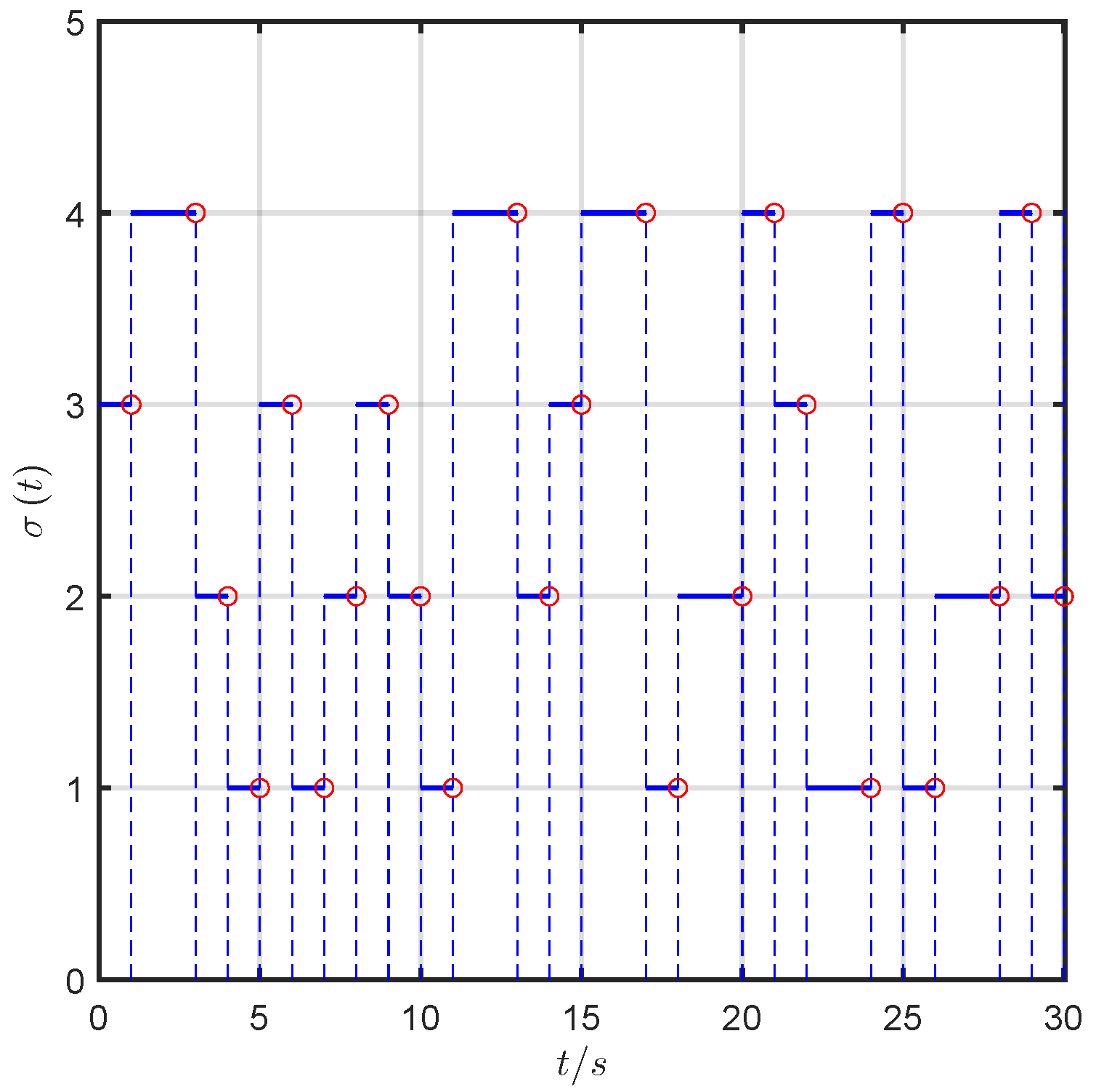
2.2. Network Topology

The network topology among the n UAVs was modeled by a directed graph $\mathcal{G}=\left(\mathcal{V},\mathcal{E}\right)$, where $\mathcal{V}=\left\{1,2,\cdots ,n\right\}$ is the vertex set representing UAVs, and $\mathcal{E}=\left\{\left(i,j\right):i,j\in \mathcal{V},i\ne j\right\}$ is the edge set between vertices. If the edge $\left(i,j\right)$ exists, UAV i can obtain the information from UAV j. A directed path from j to i is a series of finite-ordered edges $\left\{\left(i,p\right),\cdots ,\left(q,j\right)\right\}$. The graph $\mathcal{G}$ is called strongly connected if there is a directed path between any pair of vertices. To describe time-varying topologies, let $\sigma \left(t\right):\left[0,+\infty \right)\to \gamma$ denote the switching signal, whose value is the index of the network topology at time t. The switching moment $t_k\left(k\in \mathbb{N}\right)$ satisfies that $t_{k+1}-t_k⩾{\Delta }_d\left(\forall k⩾1\right)$ with ${\Delta }_d>0$. Without loss of any generality, the graph ${\mathcal{G}}_{\sigma \left(t\right)}$ is time invariant during interval $t\in \left[t_k,t_{k+1}\right)$, that is, $\sigma \left(t_k^{+}\right)=\sigma \left(t_{k+1}^{-}\right)$. ${\mathcal{E}}_{\sigma \left(t\right)}$ stands for the edge set at time t, and ${\mathcal{N}}_i^{\sigma \left(t\right)}=\left\{j\in \mathcal{V}:\left(i,j\right)\in {\mathcal{E}}_{\sigma \left(t\right)}\right\}$ stands for the neighborhood set of UAV i. Given time sequence $\left\{t_k:k\in \mathbb{N}\right\}$, varying digraphs ${\mathcal{G}}_{\sigma \left(t\right)}$ are jointly strongly connected, that is, there is some known constants $\tau >0$ such that, over time intervals $\left[l\tau ,\left(l+1\right)\tau \right)$ for $l\in \mathbb{N}$, the composite graph ${\mathcal{G}}_l$ (whose edges are the union of ${\mathcal{E}}_{\sigma \left(t_k\right)}$ for all $t_k\in \left[l\tau ,\left(l+1\right)\tau \right)$) is strongly connected. Let ${\tau }^{*}=\inf \left\{\tau >0\right\}$ denote the minimum jointly strongly connected time span. It is assumed that the network topologies among UAVs are jointly strongly connected during cooperative guidance.

2.3. Bounded-Gain Prescribed-Time Stability Criterion

Consider the following dynamic system:

$$\dot{\mathit{x}}=f(\mathit{x};\mathit{\rho }),\mathit{x}\left(0\right)={\mathit{x}}_0,$$

(5)

where $\mathit{x}:{\mathbb{R}}_{⩾0}\to {\mathbb{R}}^n$ is the system state, and the vector $\mathit{\rho }\in {\mathbb{R}}^l$ stands for the tunable parameters of (5). The function $f:{\mathbb{R}}^n\to {\mathbb{R}}^n$ may be discontinuous, such that the solutions of (5) exist and are unique in the sense of Filippov [41]. Thus, $\mathbf{\Phi }(t,{\mathit{x}}_0)$ denotes the solution of (5) starting from ${\mathit{x}}_0\in {\mathbb{R}}^n$ at $t=0$. Moreover, the origin $\mathit{x}=\mathbf{0}$ is the unique equilibrium point of (5).

A time-varying and bounded function is introduced as follows:

$${\mu }_{T_c,\kappa }=\left\{\begin{array}{cc}{\displaystyle \frac{1}{\kappa \left(T_c-t\right)}},\hfill & t<T_c\left(1-{\displaystyle \frac{1}{e^{\kappa }}}\right)\hfill \\ {\displaystyle \frac{1}{T_c}},\hfill & t⩾T_c\left(1-{\displaystyle \frac{1}{e^{\kappa }}}\right)\hfill \end{array}\right.,$$

(6)

where $\kappa >0$, and $T_c>0$ denotes the prescribed settling time. Taking the time derivative of ${\mu }_{T_c,\kappa }$ yields

$${\dot{\mu }}_{T_c,\kappa }=\left\{\begin{array}{cc}{\displaystyle \frac{1}{\kappa {\left(T_c-t\right)}^2}},\hfill & t<T_c\left(1-{\displaystyle \frac{1}{e^{\kappa }}}\right)\hfill \\ 0,\hfill & t⩾T_c\left(1-{\displaystyle \frac{1}{e^{\kappa }}}\right)\hfill \end{array}\right..$$

Lemma 1.

For System (5), if there is a continuous radially unbounded and positive definite function $V\left(\mathit{x}\right):{\mathbb{R}}^n\to \mathbb{R}$ satisfying the following condition

$$\dot{V}⩽-{\displaystyle \frac{2{\mu }_{T_c,\kappa }}{\alpha }}\left(2V+{\displaystyle \frac{1}{b}}{V}^{1-{\displaystyle \frac{\alpha }{2}}}+b{V}^{1+{\displaystyle \frac{\alpha }{2}}}\right),$$

(7)

for any solution $\mathbf{\Phi }(t,{\mathit{x}}_0)$ of System (5), where $0<\alpha <1$ and $b>0$. Then, the equilibrium of System (5) is prescribed-time stable within the settling time $T_c$.

Proof. 

Integrating both sides of (7) yields

$${\int }_0^{T\left({\mathit{x}}_0\right)}{\mu }_{T_c,\kappa }dt⩽{\int }_{V\left({\mathit{x}}_0\right)}^0{\displaystyle \frac{dV}{-\frac{2}{\alpha }\left(2V+\frac{1}{b}{V}^{1-\frac{\alpha }{2}}+b{V}^{1+\frac{\alpha }{2}}\right)}}.$$

(8)

The following proves the conclusion by contradiction. Assume that the settling-time function satisfies $T\left({\mathit{x}}_0\right)⩾T_c\left(1-1/e^{\kappa }\right)$, then (8) can be converted into

$${\int }_0^{T_c\left(1-{\displaystyle \frac{1}{e^{\kappa }}}\right)}{\displaystyle \frac{1}{\kappa \left(T_c-t\right)}}dt+{\int }_{T_c\left(1-{\displaystyle \frac{1}{e^{\kappa }}}\right)}^{T\left({\mathit{x}}_0\right)}{\displaystyle \frac{1}{T_c}}dt⩽{\displaystyle \frac{\alpha }{2}}{\int }_0^{V\left({\mathit{x}}_0\right)}{\displaystyle \frac{b{V}^{\frac{\alpha }{2}-1}}{{\left(1+b{V}^{\frac{\alpha }{2}}\right)}^2}}dV.$$

(9)

Solving (9) yields

$${\displaystyle \frac{-ln\left(\kappa \left(T_c-t\right)\right)}{\kappa }}{\mid }_0^{T_c-{\displaystyle \frac{T_c}{e^{\kappa }}}}+{\displaystyle \frac{t}{T_c}}{\mid }_{T_c-{\displaystyle \frac{T_c}{e^{\kappa }}}}^{T\left({\mathit{x}}_0\right)}⩽1-{\displaystyle \frac{1}{1+b{V}^{\frac{\alpha }{2}}\left({\mathit{x}}_0\right)}}<1.$$

(10)

Upon rearrangement of (10), one has

$$T\left({\mathit{x}}_0\right)<T_c\left(1-{\displaystyle \frac{1}{e^{\kappa }}}\right).$$

This is a contradiction. Thus, one can obtain $T\left({\mathit{x}}_0\right)<T_c\left(1-1/e^{\kappa }\right)<T_c$.    □

Remark 1.

Our approach was unlike the pioneering work on prescribed-time stability theory in [27], where the time-varying function $\mu \left(t\right)$ with the properties that $\mu \left(T_c\right)=+\infty$ introduces the infinite-gain challenge. To solve this issue, the time-varying Function (6) was constructed, whose switching point can be placed at $T_c\left(1-1/e^{\kappa }\right)$ by virtue of Condition (7) in Lemma 1. This configuration ensures ${\sup }_{t⩾0}{\mu }_{T_c,\kappa }=e^{\kappa }/\left(\kappa T_c\right)$, thereby establishing a bounded-gain prescribed-time stability criterion in Lemma 1. Note that Lemma 1 indicates that System (5) satisfying Condition (7) can achieve convergence before the switching point $T_c\left(1-1/e^{\kappa }\right)$. Thus, the discontinuities of ${\mu }_{T_c,\kappa }$ and its derivative do not affect the prescribed-time convergence property of this criterion.

Remark 2.

It is noteworthy that, when $\kappa =0$, Condition (7) converts to the predefined-time stability condition in [25], where the gain is time-invariant. Since Lemma 1 demonstrates $T\left({\mathit{x}}_0\right)<T_c\left(1-1/e^{\kappa }\right)$, (8) can be transformed into

$${\int }_0^{T\left({\mathit{x}}_0\right)}{\displaystyle \frac{1}{\kappa \left(T_c-t\right)}}dt⩽{\displaystyle \frac{\alpha }{2}}{\int }_0^{V\left({\mathit{x}}_0\right)}{\displaystyle \frac{b{V}^{\frac{\alpha }{2}-1}}{{\left(1+b{V}^{\frac{\alpha }{2}}\right)}^2}}dV.$$

By simplifying the above equation, one can obtain $T\left({\mathit{x}}_0\right)⩽T_c\left(1-1/e^{\kappa \left(1-1/\left(1+b{V}^{\alpha /2}\left({\mathit{x}}_0\right)\right)\right)}\right)<T_c$. From the term $1/e^{\kappa \left(1-1/\left(1+b{V}^{\alpha /2}\left({\mathit{x}}_0\right)\right)\right)}$, it can be found that the deviation between the actual and prescribed convergence times is influenced by the initial state ${\mathit{x}}_0$, as well as parameters α, b, and κ. Interestingly, it is noted that ${lim}_{\kappa \to +\infty }1/e^{\kappa \left(1-1/\left(1+b{V}^{\alpha /2}\left({\mathit{x}}_0\right)\right)\right)}=0$, which indicates that choosing a large parameter κ can effectively reduce the conservativeness of the prescribed time. In summary, Lemma 1 establishes a bridge between the predefined-time stability and prescribed-time stability through the parameter κ, inheriting their respective advantages: the boundedness of the gain and the accuracy of the prescribed settling time.

3. Design of the PDOs

To facilitate the subsequent design of the PRCG law, PDOs were constructed, as shown in this section, to compensate for the unknown acceleration of the target.

For UAV i$\left(i\in \mathcal{V}\right)$, the time-to-go $t_{\mathrm{go}}^i$ is estimated by $t_{\mathrm{go}}^i=-r_i/{\dot{r}}_i$, defining ${\Theta }_1^i={\theta }_i-{\theta }_D^i$, ${\Theta }_2^i={\dot{\theta }}_i$, ${\Psi }_1^i={\psi }_i-{\psi }_D^i$, ${\Psi }_2^i={\dot{\psi }}_i$. Consequently, according to (1), (2), and (3), the guidance system can be rewritten as

$${\dot{t}}_f^i={\left({\displaystyle \frac{r_i{\dot{\theta }}_i}{{\dot{r}}_i}}\right)}^2+{\left({\displaystyle \frac{r_i{\dot{\psi }}_{i}cos{\theta }_i}{{\dot{r}}_i}}\right)}^2-{\displaystyle \frac{r_i}{{\left({\dot{r}}_i\right)}^2}}{a}_{Mx}^i+{\displaystyle \frac{r_i}{{\left({\dot{r}}_i\right)}^2}}{a}_{Tx}^i,$$

(11)

$$\left\{\begin{array}{c}{\dot{\Theta }}_1^i={\Theta }_2^i\hfill \\ {\dot{\Theta }}_2^i=A_y^i+B_y^i{a}_{My}^i-B_y^i{a}_{Ty}^i\hfill \end{array}\right.,$$

(12)

$$\left\{\begin{array}{c}{\dot{\Psi }}_1^i={\Psi }_2^i\hfill \\ {\dot{\Psi }}_2^i=A_z^i+B_z^i{a}_{Mz}^i-B_z^i{a}_{Tz}^i\hfill \end{array}\right.,$$

(13)

where

$$A_y^i=-{\displaystyle \frac{2{\dot{r}}_i{\dot{\theta }}_i}{r_i}}-{\left({\dot{\psi }}_i\right)}^{2}sin{\theta }_{i}cos{\theta }_i,B_y^i=-{\displaystyle \frac{1}{r_i}},$$

$$A_z^i=-{\displaystyle \frac{2{\dot{r}}_i{\dot{\psi }}_i}{r_i}}+2{\dot{\theta }}_i{\dot{\psi }}_{i}tan{\theta }_i,B_z^i={\displaystyle \frac{1}{r_{i}cos{\theta }_i}}.$$

As shown in the following, PDOs were designed for estimating the unknown target acceleration components $a_{Tx}^i$, $a_{Ty}^i$, and $a_{Tz}^i$. Firstly, from (11), (12), and (13), consider the following three systems

$${\dot{\widehat{t}}}_f^i={\left({\displaystyle \frac{r_i{\dot{\theta }}_i}{{\dot{r}}_i}}\right)}^2+{\left({\displaystyle \frac{r_i{\dot{\psi }}_{i}cos{\theta }_i}{{\dot{r}}_i}}\right)}^2-{\displaystyle \frac{r_i}{{\left({\dot{r}}_i\right)}^2}}{a}_{Mx}^i+{\varsigma }_o^x{\xi }_x^i,$$

(14)

$${\dot{\widehat{\Theta }}}_2^i=A_y^i+B_y^i{a}_{My}^i+{\varsigma }_o^y{\xi }_y^i,$$

(15)

$${\dot{\widehat{\Psi }}}_2^i=A_z^i+B_z^i{a}_{Mz}^i+{\varsigma }_o^z{\xi }_z^i,$$

(16)

where ${\xi }_x^i=t_f^i-{\widehat{t}}_f^i$, ${\xi }_y^i={\Theta }_2^i-{\widehat{\Theta }}_2^i$, ${\xi }_z^i={\Psi }_2^i-{\widehat{\Psi }}_2^i$, ${\varsigma }_o^x>0$, ${\varsigma }_o^y>0$ and ${\varsigma }_o^z>0$. Then, three PDOs are constructed as

$${\widehat{a}}_{Tx}^i={\displaystyle \frac{{\left({\dot{r}}_i\right)}^2}{r_i}}\left({\varsigma }_o^x{\widehat{\xi }}_x^i+{\dot{\xi }}_x^i\right),$$

(17)

$${\widehat{a}}_{Ty}^i=-\left({\varsigma }_o^y{\widehat{\xi }}_y^i+{\dot{\xi }}_y^i\right)/B_y^i,$$

(18)

$${\widehat{a}}_{Tz}^i=-\left({\varsigma }_o^z{\widehat{\xi }}_z^i+{\dot{\xi }}_z^i\right)/B_z^i,$$

(19)

where ${\widehat{a}}_{Tx}^i$, ${\widehat{a}}_{Ty}^i$, and ${\widehat{a}}_{Tz}^i$ are the estimations of $a_{Tx}^i$, $a_{Ty}^i$, and $a_{Tz}^i$, respectively. Finally, ${\widehat{\xi }}_x^i$ is the estimation of ${\xi }_x^i$ given by

$${\dot{\widehat{\xi }}}_x^i={\dot{\xi }}_x^i+{\displaystyle \frac{{\mu }_{T_o^x,{\kappa }_o^x}}{{\alpha }_o^x}}\left(2{\tilde{\xi }}_x^i+{\displaystyle \frac{1}{b_o^x}}{\lfloor {\tilde{\xi }}_x^i\rceil }^{1-{\alpha }_o^x}+b_o^x{\lfloor {\tilde{\xi }}_x^i\rceil }^{1+{\alpha }_o^x}\right),$$

(20)

where ${\tilde{\xi }}_x^i={\xi }_x^i-{\widehat{\xi }}_x^i$ is the estimation error, $0<{\alpha }_o^x<1$, $b_o^x>0$, ${\kappa }_o^x>0$, and $T_o^x>0$ is a prescribed settling time. Moreover, ${\widehat{\xi }}_y^i$ is the estimation of ${\xi }_y^i$ given by

$${\dot{\widehat{\xi }}}_y^i={\dot{\xi }}_y^i+{\displaystyle \frac{{\mu }_{T_o^y,{\kappa }_o^y}}{{\alpha }_o^y}}\left(2{\tilde{\xi }}_y^i+{\displaystyle \frac{1}{b_o^y}}{\lfloor {\tilde{\xi }}_y^i\rceil }^{1-{\alpha }_o^y}+b_o^y{\lfloor {\tilde{\xi }}_y^i\rceil }^{1+{\alpha }_o^y}\right),$$

(21)

where ${\tilde{\xi }}_y^i={\xi }_y^i-{\widehat{\xi }}_y^i$ is the estimation error, $0<{\alpha }_o^y<1$, $b_o^y>0$, ${\kappa }_o^y>0$, and $T_o^y>0$ is a prescribed settling time. Furthermore, ${\widehat{\xi }}_z^i$ is the estimation of ${\xi }_z^i$ given by

$${\dot{\widehat{\xi }}}_z^i={\dot{\xi }}_z^i+{\displaystyle \frac{{\mu }_{T_o^z,{\kappa }_o^z}}{{\alpha }_o^z}}\left(2{\tilde{\xi }}_z^i+{\displaystyle \frac{1}{b_o^z}}{\lfloor {\tilde{\xi }}_z^i\rceil }^{1-{\alpha }_o^z}+b_o^z{\lfloor {\tilde{\xi }}_z^i\rceil }^{1+{\alpha }_o^z}\right),$$

(22)

where ${\tilde{\xi }}_z^i={\xi }_z^i-{\widehat{\xi }}_z^i$ is the estimation error, $0<{\alpha }_o^z<1$, $b_o^z>0$, ${\kappa }_o^z>0$, and $T_o^z>0$ is a prescribed settling time.

Lemma 2.

The PDOs (17), (18), and (19) can converge to $a_{Tx}^i$, $a_{Ty}^i$, and $a_{Tz}^i$ within the prescribed time $T_o^x$, $T_o^y$, and $T_o^z$, respectively.

Proof. 

Firstly, it is proven that PDO (17) can converge to $a_{Tx}^i$ within the prescribed time $T_o^x$. According to (20), the derivative of the estimation error ${\tilde{\xi }}_x^i$ can be given as

$${\dot{\tilde{\xi }}}_x^i=-{\displaystyle \frac{{\mu }_{T_o^x,{\kappa }_o^x}}{{\alpha }_o^x}}\left(2{\tilde{\xi }}_x^i+{\displaystyle \frac{1}{b_o^x}}{\lfloor {\tilde{\xi }}_x^i\rceil }^{1-{\alpha }_o^x}+b_o^x{\lfloor {\tilde{\xi }}_x^i\rceil }^{1+{\alpha }_o^x}\right).$$

(23)

Construct a Lyapunov function as $V_{ox}^i={\left({\tilde{\xi }}_x^i\right)}^2$. Differentiating $V_{ox}^i$ along the trajectories of (23) gives that

$${\dot{V}}_{ox}^i=-{\displaystyle \frac{2{\mu }_{T_o^x,{\kappa }_o^x}}{{\alpha }_o^x}}\left(2V_{ox}^i+{\displaystyle \frac{1}{b_o^x}}{\left(V_{ox}^i\right)}^{1-{\displaystyle \frac{{\alpha }_o^x}{2}}}+b_o^x{\left(V_{ox}^i\right)}^{1+{\displaystyle \frac{{\alpha }_o^x}{2}}}\right).$$

(24)

According to Lemma 1, it can be concluded that ${\tilde{\xi }}_x^i\left(t\right)=0$ for all $t⩾T_o^x$. By recalling (11), (14), and (17), the acceleration estimation error can be calculated as follows

$$a_{Tx}^i-{\widehat{a}}_{Tx}^i=a_{Tx}^i-{\displaystyle \frac{{\left({\dot{r}}_i\right)}^2}{r_i}}\left({\varsigma }_o^x{\widehat{\xi }}_x^i+{\dot{\xi }}_x^i\right)={\displaystyle \frac{{\left({\dot{r}}_i\right)}^2{\varsigma }_o^x}{r_i}}{\tilde{\xi }}_x^i.$$

Thus, it can be obtained that PDO (17) can converge to $a_{Tx}^i$ in the prescribed time $T_o^x$.

The proof procedures about PDOs (18) and (19) were similar to those of the PDO (17), so they are omitted here.    □

Remark 3.

In contrast to the appointed-time extended state observer in [36], which slightly sacrifices estimation accuracy to avoid infinite gain in practical applications, the PDOs based on the bounded-gain prescribed-time stability criterion eliminated such limitations and can provide higher estimation accuracy. Moreover, both the configuration of the settling time for PDOs and related operational processes were found to be independent of a priori information about the target, which makes it highly user-friendly.

4. Design of the PRCG Law

In this section, a PRCG law with the spatiotemporal constraint is proposed by designing tangential and normal acceleration commands, and the corresponding prescribed-time stability analysis is provided.

4.1. Tangential Acceleration Command Design

The tangential acceleration command was designed to achieve the arrival time consensus among UAVs within a prescribed time.

For UAV i$\left(i\in \mathcal{V}\right)$, a distributed convex hull observer (DCHO) is constructed as

$$\left\{\begin{array}{c}{\overline{t}}_f^i\left(t\right)=max\left[{\overline{t}}_f^i\left(t^{-}\right),\underset{j\in {\mathcal{N}}_i^{\sigma \left(t\right)}}{\max }{\overline{t}}_f^j\left(t\right)\right]\hfill \\ {\underline{t}}_f^i\left(t\right)=min\left[{\underline{t}}_f^i\left(t^{-}\right),\underset{j\in {\mathcal{N}}_i^{\sigma \left(t\right)}}{\min }{\underline{t}}_f^j\left(t\right)\right]\hfill \end{array}\right.,$$

(25)

where ${\overline{t}}_f^i\left(0\right)={\underline{t}}_f^i\left(0\right)=t_f^i\left(0\right)$.

Definition 1.

The $t^{*}$ is said to be the first arrival steady state time if $t^{*}=\inf \left\{t>0:{\overline{t}}_f^i\left(t\right)=\right.$$\left.{\overline{t}}_f^i\left(t+\Delta t\right),{\underline{t}}_f^i\left(t\right)={\underline{t}}_f^i\left(t+\Delta t\right),\forall \Delta t>0,\forall i\in \mathcal{V}\right\}$.

Under jointly strongly connected topologies, the tangential acceleration command $a_{Mx}^i$ is designed as

$$a_{Mx}^i=r_i{\left({\dot{\theta }}_i\right)}^2+r_i{\left({\dot{\psi }}_L^{i}cos{\theta }_i\right)}^2+{\displaystyle \frac{{\left({\dot{r}}_i\right)}^2}{r_i}}{u}_{Mx}^i+{\widehat{a}}_{Tx}^i,$$

(26)

where ${\widehat{a}}_{Tx}^i$ is obtained by PDO (17) and

$$u_{Mx}^i=-{\displaystyle \frac{{\mu }_{T_x,{\kappa }_x}}{{\alpha }_x}}\left(2(t_c^i-t_f^i)+{\displaystyle \frac{1}{b_x}}{\lfloor t_c^i-t_f^i\rceil }^{1-{\alpha }_x}+b_x{\lfloor t_c^i-t_f^i\rceil }^{1+{\alpha }_x}\right),$$

(27)

where $t_c^i=\varrho {\overline{t}}_f^i+\left(1-\varrho \right){\underline{t}}_f^i$, $0⩽\varrho ⩽1$, $0<{\alpha }_x<1$, $b_x>0$, ${\kappa }_x>0$, and $T_x\left(T_x>T_o^x\right)$ is a prescribed settling time.

Lemma 3.

For the guidance System (11) with the tangential acceleration Command (26), PDO (17) and DCHO (25), if network topologies are jointly strongly connected, then there are ${\overline{t}}_f^i\left(t^{*}\right)={max}_{i\in \mathcal{V}}{\overline{t}}_f^i\left(T_o^x\right)$, ${\underline{t}}_f^i\left(t^{*}\right)={min}_{i\in \mathcal{V}}{\underline{t}}_f^i\left(T_o^x\right)$, and $t^{*}⩽n{\tau }^{*}+T_o^x$.

Proof. 

According to Lemma 2, PDO (17) can guarantee that $a_{Tx}^i={\widehat{a}}_{Tx}^i$ for all $t⩾T_o^x$ and $i\in \mathcal{V}$. Therefore, for $i\in \mathcal{V}$, when $t⩾T_o^x$, one derives that ${\dot{t}}_f^i=-u_{Mx}^i$ in virtue of (11) and (26). Due to $t_c^i=\varrho {\overline{t}}_f^i+\left(1-\varrho \right){\underline{t}}_f^i$, one obtains that ${\underline{t}}_f^i⩽t_c^i⩽{\overline{t}}_f^i$. Once $t_f^i={\overline{t}}_f^i$, there is $u_{Mx}^i⩾0$ and, in turn, ${\dot{t}}_f^i⩽0$, which means that $t_f^i⩽{\overline{t}}_f^i$ holds for all $t⩾T_o^x$. Similarly, once $t_f^i={\underline{t}}_f^i$, there is $u_{Mx}^i⩽0$ and, in turn, ${\dot{t}}_f^i⩾0$, which means that $t_f^i⩾{\underline{t}}_f^i$ holds for all $t⩾T_o^x$. Consequently, it can be inferred that ${\underline{t}}_f^i⩽t_f^i⩽{\overline{t}}_f^i$ for all $t⩾T_o^x$. Given the update strategy of DCHO (25), it follows that ${\overline{t}}_f^i$ is monotonically increasing and upper bounded by ${max}_{i\in \mathcal{V}}{\overline{t}}_f^i\left(T_o^x\right)$ and that ${\underline{t}}_f^i$ is monotonically decreasing and lower bounded by ${min}_i{\underline{t}}_f^i\left(T_o^x\right)$. Thus, there are ${\overline{t}}_f^i\left(t^{*}\right)={max}_{i\in \mathcal{V}}{\overline{t}}_f^i\left(T_o^x\right)$ and ${\underline{t}}_f^i\left(t^{*}\right)={min}_{i\in \mathcal{V}}{\underline{t}}_f^i\left(T_o^x\right)$. Moreover, according to the definition of joint strongly connected topologies, both ${\overline{t}}_f^i$ and ${\underline{t}}_f^i$$\left(i\in \mathcal{V}\right)$ converge to their consensus values within the time $n{\tau }^{*}$ once $a_{Tx}^i={\widehat{a}}_{Tx}^i$, i.e., $t^{*}⩽n{\tau }^{*}+T_o^x$.    □

Remark 4.

The design objective of DCHO (25) was to obtain the convex hull formed by the estimations of arrival times for UAVs since the initial time. Under the tangential acceleration Command (26), Lemma 3 proves that this convex hull possesses invariance once PDO (17) converges. This fact ensures the existence of the first arrival steady state time $t^{*}$, thereby providing the possibility for achieving consensus on the arrival times of UAVs within a prescribed time. The results of Lemma 3 indicate that the first arrival steady state time $t^{*}$ of the DCHO is influenced by three factors: the prescribed time $T_o^x$ of PDO (17), the UAV numbers n, and the minimum jointly strongly connected time span ${\tau }^{*}$. Since the prescribed time $T_o^x$ cannot be ignored and the UAV numbers n are determined by the mission, the first steady state arrival time $t^{*}$ can only be adjusted by the minimum jointly strongly connected time span ${\tau }^{*}$. Generally, ${\tau }^{*}$ can be reduced by enhancing communication links or decreasing the communication period, which will lead to an increase in communication load. Consequently, there is a trade-off between the DCHO’s first steady state arrival time $t^{*}$ and the communication load. It should be noted that the directed jointly strongly connected topologies represent the least conservative topological requirement for achieving a finite-time consensus [42]. In practice, such extreme communication conditions are rare, so $t^{*}$ is typically smaller. Specifically, for any directed strongly connected topology, ${\tau }^{*}$ equals a communication period, implying that DCHO (25) can reach consensus values almost instantaneously.

Theorem 1.

For the guidance System (11), if network topologies are jointly strongly connected with $t^{*}<T_x$, UAVs can make their arrival times reach consensus within the prescribed time $T_x$ using the tangential acceleration Command (26) with PDO (17) and DCHO (25).

Proof. 

According to Lemma 2, there is $a_{Tx}^i={\widehat{a}}_{Tx}^i$ for all $t⩾T_o^x$. Based on Lemma 3, one can obtain that $t_c^i\left(t\right)=\varrho {\overline{t}}_f^i\left(t^{*}\right)+\left(1-\varrho \right){\underline{t}}_f^i\left(t^{*}\right)$ for all $t⩾t^{*}$, which implies that $t_c^i$ is time-invariant and $t_c^1\left(t\right)=t_c^2\left(t\right)=\cdots =t_c^n\left(t\right)$ when $t⩾t^{*}$. Subsequently, construct a Lyapunov function $V_x^i={\left(t_f^i-t_c^i\right)}^2$. The time derivative of $V_x^i$ can be obtained as

$$\begin{array}{cc}\hfill {\dot{V}}_x^i=& {\displaystyle \frac{2{\mu }_{T_x,{\kappa }_x}}{{\alpha }_x}}\left(t_f^i-t_c^i\right)\left(2(t_c^i-t_f^i)+{\displaystyle \frac{1}{b_x}}{\lfloor t_c^i-t_f^i\rceil }^{1-{\alpha }_x}+b_x{\lfloor t_c^i-t_f^i\rceil }^{1+{\alpha }_x}\right)\hfill \\ \hfill =& -{\displaystyle \frac{2{\mu }_{T_x,{\kappa }_x}}{{\alpha }_x}}\left(2V_x^i+{\displaystyle \frac{1}{b_x}}{\left(V_x^i\right)}^{1-{\displaystyle \frac{{\alpha }_x}{2}}}+b_x{\left(V_x^i\right)}^{1+{\displaystyle \frac{{\alpha }_x}{2}}}\right).\hfill \end{array}$$

By Lemma 1, the equilibrium of $V_x^i=0$, i.e., $t_f^i=t_c^i$, can achieve stability within the prescribed time $T_x$.    □

Remark 5.

According to the proof of Theorem 1, the consensus value of the arrival times for all UAVs is $t_c^i\left(t\right)=\varrho {\overline{t}}_f^i\left(t^{*}\right)+\left(1-\varrho \right){\underline{t}}_f^i\left(t^{*}\right)$. Lemma 3 states that ${\overline{t}}_f^i\left(t^{*}\right)={max}_{i\in \mathcal{V}}{\overline{t}}_f^i\left(T_o^x\right)$ and ${\underline{t}}_f^i\left(t^{*}\right)={min}_{i\in \mathcal{V}}{\underline{t}}_f^i\left(T_o^x\right)$. Consequently, the consensus value of the arrival times is determined by the state of DCHO (25) at time $T_o^x$. Especially when the target acceleration is zero, $T_o^x$ can be set to zero, and, in this case, the consensus value of the arrival times is determined by the estimation of initial arrival times. In addition, it is worth noting that $t_c^i=\varrho {\overline{t}}_f^i+\left(1-\varrho \right){\underline{t}}_f^i$ indicates that $t_c^i$ is a convex combination of ${\overline{t}}_f^i$ and ${\underline{t}}_f^i$, and the selection of the parameter ϱ governs the cooperative behavior of UAVs. Specifically, when $\varrho =0$ and $\varrho =1$, the consensus value of arrival times will converge to the minimum and maximum arrival time among UAVs, respectively, that is, as ϱ increases within the interval $\left[0,1\right]$, the arrival time of UAVs to the target becomes longer. Thus, in applications, one can select an appropriate parameter ϱ according to the time urgency of the cooperative mission.

Corollary 1.

Consider the scenario where some UAVs may become faulty. For the guidance System (11), if the below conditions hold, then the surviving UAVs can make their arrival times reach consensus within the prescribed time $T_x$ using the tangential acceleration Command (26) with PDO (17) and DCHO (25):

(i) 

During phases when no UAV is faulty, the network topologies of UAVs are jointly strongly connected with $t^{*}<T_x$;

(ii) 

After some UAVs become faulty, the network topologies of surviving UAVs remain jointly strongly connected.

Proof. 

The proof of this corollary can be completed by directly verifying whether the surviving UAVs satisfy the sufficient conditions of Theorem 1. According to the given conditions of the corollary, it can be seen that the surviving UAVs, as a subset of the original UAVs, satisfy the sufficient conditions of Theorem 1, and thus the corollary holds.    □

Remark 6.

For surviving UAVs with the tangential acceleration Command (26), the convex hull formed by the estimations of arrival times still possesses invariance once PDO (17) converges. Consequently, by virtue of DCHO (25), the PRCG law can achieve the cooperative guidance among surviving UAVs without the knowledge of faulty UAVs or any fault diagnosis procedure.

4.2. Normal Acceleration Command Design

Two normal acceleration commands were designed so that each UAV can satisfy the LOS angle constraints within a prescribed time.

Choose a piecewise continuous function as follows:

$${\mathcal{X}}_{\alpha ,ϵ}\left(\zeta \right)=\left\{\begin{array}{c}{\lfloor \zeta \rceil }^{1-\alpha },\left|\zeta \right|>ϵ\hfill \\ {\mathcal{X}}_0\zeta +{\mathcal{X}}_1{\lfloor \zeta \rceil }^2,\left|\zeta \right|⩽ϵ\hfill \end{array}\right.,$$

(28)

where $0<\alpha <1$, $ϵ>0$, ${\mathcal{X}}_0=\left(1+\alpha \right){ϵ}^{-\alpha }$, and ${\mathcal{X}}_1=-\alpha {ϵ}^{-\left(1+\alpha \right)}$. Taking the derivative of ${\mathcal{X}}_{\alpha ,ϵ}$ with respect to $\zeta$ yields

$${\dot{\mathcal{X}}}_{\alpha ,ϵ}\left(\zeta \right)=\left\{\begin{array}{c}\left(1-\alpha \right){\left|\zeta \right|}^{-\alpha }\dot{\zeta },\left|\zeta \right|>ϵ\hfill \\ {\mathcal{X}}_0\dot{\zeta }+2{\mathcal{X}}_1\left|\zeta \right|\dot{\zeta },\left|\zeta \right|⩽ϵ\hfill \end{array}\right..$$

(29)

For UAV i$\left(i\in \mathcal{V}\right)$, a prescribed-time nonsingular sliding mode surface is constructed as

$$s_y^i={\Theta }_2^i+{\displaystyle \frac{{\mu }_{T_{y1},{\kappa }_{y1}}}{{\alpha }_{y1}}}\left(2{\Theta }_1^i+{\displaystyle \frac{1}{b_{y1}}}{\mathcal{X}}_{{\alpha }_{y1},{ϵ}_y}\left({\Theta }_1^i\right)+b_{y1}{\lfloor {\Theta }_1^i\rceil }^{1+{\alpha }_{y1}}\right),$$

(30)

where $0<{\alpha }_{y1}<1$, $b_{y1}>0$, ${ϵ}_y>0$, ${\kappa }_{y1}>0$, and $T_{y1}\left(T_{y1}>T_o^y\right)$ is a prescribed settling time. The time derivative of $s_y^i$ can be obtained as

$$\begin{array}{cc}\hfill {\dot{s}}_y^i=& {\displaystyle \frac{{\mu }_{T_{y1},{\kappa }_{y1}}}{{\alpha }_{y1}}}\left(2{\dot{\Theta }}_1^i+{\displaystyle \frac{1}{b_{y1}}}{\dot{\mathcal{X}}}_{{\alpha }_{y1},{ϵ}_y}\left({\Theta }_1^i\right)+b_{y1}\left(1+{\alpha }_{y1}\right){\left|{\Theta }_1^i\right|}^{{\alpha }_{y1}}{\dot{\Theta }}_1^i\right)\hfill \\ \hfill +& {\displaystyle \frac{{\dot{\mu }}_{T_{y1},{\kappa }_{y1}}}{{\alpha }_{y1}}}\left(2{\Theta }_1^i+{\displaystyle \frac{1}{b_{y1}}}{\mathcal{X}}_{{\alpha }_{y1},{ϵ}_y}\left({\Theta }_1^i\right)+b_{y1}{\lfloor {\Theta }_1^i\rceil }^{1+{\alpha }_{y1}}\right)\hfill \\ \hfill +& A_y^i+B_y^i{a}_{My}^i-B_y^i{a}_{Ty}^i.\hfill \end{array}$$

(31)

Then, a prescribed-time convergence reaching law is selected in the following form:

$${\dot{s}}_y^i=-{\displaystyle \frac{{\mu }_{T_{y2},{\kappa }_{y2}}}{{\alpha }_{y2}}}\left(2s_y^i+{\displaystyle \frac{1}{b_{y2}}}{\lfloor s_y^i\rceil }^{1-{\alpha }_{\theta 2}}+b_{y2}{\lfloor s_y^i\rceil }^{1+{\alpha }_{y2}}\right),$$

(32)

where $0<{\alpha }_{y2}<1$, $b_{y2}>0$, ${\kappa }_{y2}>0$, and $T_{y2}\left(T_o^y<T_{y2}<T_{y1}\right)$ is a prescribed settling time. Based on the sliding mode Surface (30) and the reaching Law (32), the normal acceleration $a_{My}^i$ is designed as

$$\begin{array}{cc}\hfill a_{My}^i=& -{\displaystyle \frac{{\mu }_{T_{y2},{\kappa }_{y2}}}{{\alpha }_{y2}{B}_y^i}}\left(2s_y^i+{\displaystyle \frac{1}{b_{y2}}}{\lfloor s_y^i\rceil }^{1-{\alpha }_{y2}}+b_{y2}{\lfloor s_y^i\rceil }^{1+{\alpha }_{y2}}\right)\hfill \\ \hfill -& {\displaystyle \frac{{\mu }_{T_{y1},{\kappa }_{y1}}}{{\alpha }_{y1}{B}_y^i}}\left(2{\dot{\Theta }}_1^i+{\displaystyle \frac{1}{b_{y1}}}{\dot{\mathcal{X}}}_{{\alpha }_{y1},{ϵ}_y}\left({\Theta }_1^i\right)+b_{y1}\left(1+{\alpha }_{y1}\right){\left|{\Theta }_1^i\right|}^{{\alpha }_{y1}}{\dot{\Theta }}_1^i\right)\hfill \\ \hfill -& {\displaystyle \frac{{\dot{\mu }}_{T_{y1},{\kappa }_{y1}}}{{\alpha }_{y1}{B}_y^i}}\left(2{\Theta }_1^i+{\displaystyle \frac{1}{b_{y1}}}{\mathcal{X}}_{{\alpha }_{y1},{ϵ}_y}\left({\Theta }_1^i\right)+b_{y1}{\lfloor {\Theta }_1^i\rceil }^{1+{\alpha }_{y1}}\right)-{\displaystyle \frac{A_y^i}{B_y^i}}+{\widehat{a}}_{Ty}^i,\hfill \end{array}$$

(33)

where ${\widehat{a}}_{Ty}^i$ is given by PDO (18).

Similarly, a prescribed-time nonsingular terminal sliding mode surface was constructed as

$$s_z^i={\Psi }_2^i+{\displaystyle \frac{{\mu }_{T_{z1},{\kappa }_{z1}}}{{\alpha }_{z1}}}\left(2{\Psi }_1^i+{\displaystyle \frac{1}{b_{z1}}}{\mathcal{X}}_{{\alpha }_{z1},{ϵ}_z}\left({\Psi }_1^i\right)+b_{z1}{\lfloor {\Psi }_1^i\rceil }^{1+{\alpha }_{z1}}\right),$$

(34)

where $0<{\alpha }_{z1}<1$, $b_{z1}>0$, ${ϵ}_z>0$, ${\kappa }_{z1}>0$, and $T_{z1}\left(T_{z1}>T_o^z\right)$ is a prescribed settling time. The normal acceleration command $a_{Mz}^i$ is designed as

$$\begin{array}{cc}\hfill a_{Mz}^i=& -{\displaystyle \frac{{\mu }_{T_{z2},{\kappa }_{z2}}}{{\alpha }_{z2}{B}_z^i}}\left(2s_z^i+{\displaystyle \frac{1}{b_{z2}}}{\lfloor s_z^i\rceil }^{1-{\alpha }_{z2}}+b_{z2}{\lfloor s_z^i\rceil }^{1+{\alpha }_{z2}}\right)\hfill \\ \hfill -& {\displaystyle \frac{{\mu }_{T_{z1},{\kappa }_{z1}}}{{\alpha }_{z1}{B}_z^i}}\left(2{\dot{\Psi }}_1^i+{\displaystyle \frac{1}{b_{z1}}}{\dot{\mathcal{X}}}_{{\alpha }_{z1},{ϵ}_z}\left({\Psi }_1^i\right)+b_{z1}\left(1+{\alpha }_{z1}\right){\left|{\Psi }_1^i\right|}^{{\alpha }_{z1}}{\dot{\Psi }}_1^i\right)\hfill \\ \hfill -& {\displaystyle \frac{{\dot{\mu }}_{T_{z1},{\kappa }_{z1}}}{{\alpha }_{z1}{B}_z^i}}\left(2{\Psi }_1^i+{\displaystyle \frac{1}{b_{z1}}}{\mathcal{X}}_{{\alpha }_{z1},{ϵ}_z}\left({\Psi }_1^i\right)+b_{z1}{\lfloor {\Psi }_1^i\rceil }^{1+{\alpha }_{z1}}\right)-{\displaystyle \frac{A_z^i}{B_z^i}}+{\widehat{a}}_{Tz}^i,\hfill \end{array}$$

(35)

where $0<{\alpha }_{z2}<1$, $b_{z2}>0$, ${\kappa }_{z2}>0$, $T_{z2}\left(T_o^z<T_{z2}<T_{z1}\right)$ is a prescribed settling time, and ${\widehat{a}}_{Tz}^i$ is given by PDO (19).

Theorem 2.

Consider the guidance System (12), the normal acceleration Command (33) with PDO (18) can guarantee that the LOS elevation angle ${\theta }_i$ can converge to the prescribed neighborhood ${\mathcal{B}}_{{ϵ}_y}\left({\theta }_D^i\right)$ within the prescribed time $T_{y1}^i$.

Proof. 

Substituting (33) into (31) yields

$${\dot{s}}_y^i=-{\displaystyle \frac{{\mu }_{T_{y2},{\kappa }_{y2}}}{{\alpha }_{y2}}}\left(2s_y^i+{\displaystyle \frac{1}{b_{y2}}}{\lfloor s_y^i\rceil }^{1-{\alpha }_{y2}}+b_{y2}{\lfloor s_y^i\rceil }^{1+{\alpha }_{y2}}\right)+B_y^i\left({\widehat{a}}_{Ty}^i-a_{Ty}^i\right).$$

(36)

Based on Lemma 2, it can be found that ${\widehat{a}}_{Ty}^i-a_{Ty}^i=0$ for all $t⩾T_o^y$. Thus, when $t⩾T_o^y$, (36) can be converted into

$${\dot{s}}_y^i=-{\displaystyle \frac{{\mu }_{T_{y2},{\kappa }_{y2}}}{{\alpha }_{y2}}}\left(2s_y^i+{\displaystyle \frac{1}{b_{y2}}}{\lfloor s_y^i\rceil }^{1-{\alpha }_{y2}}+b_{y2}{\lfloor s_y^i\rceil }^{1+{\alpha }_{y2}}\right).$$

(37)

Construct the Lyapunov function $V_y^i={\left(s_y^i\right)}^2$ and the time derivative of $V_y^i$ along the trajectories of (37), which can be given as

$${\dot{V}}_y^i=-{\displaystyle \frac{2{\mu }_{T_{y2},{\kappa }_{y2}}}{{\alpha }_{y2}}}\left(2V_y^i+{\displaystyle \frac{1}{b_{y2}}}{\left(V_y^i\right)}^{1-{\displaystyle \frac{{\alpha }_{y2}}{2}}}+b_{y2}{\left(V_y^i\right)}^{1+{\displaystyle \frac{{\alpha }_{y2}}{2}}}\right).$$

(38)

According to Lemma 1, the equilibrium of $V_y^i$, i.e., $s_y^i=0$, can achieve stability within the prescribed time $T_{y2}$.

From (30), when $s_y^i=0$, one has

$${\Theta }_2^i=-{\displaystyle \frac{{\mu }_{T_{y1},{\kappa }_{y1}}}{{\alpha }_{y1}}}\left(2{\Theta }_1^i+{\displaystyle \frac{1}{b_{y1}}}{\mathcal{X}}_{{\alpha }_{y1},{ϵ}_y}\left({\Theta }_1^i\right)+b_{y1}{\lfloor {\Theta }_1^i\rceil }^{1+{\alpha }_{y1}}\right).$$

Consider the Lyapunov function ${\Xi }_y^i={\left({\Theta }_1^i\right)}^2$ and the time derivative of ${\Xi }_y^i$, which can be obtained as follows:

$${\dot{\Xi }}_y^i=-{\displaystyle \frac{2{\mu }_{T_{y1},{\kappa }_{y1}}}{{\alpha }_{y1}}}\left(2{\left({\Theta }_1^i\right)}^2+{\displaystyle \frac{1}{b_{y1}}}{\mathcal{X}}_{{\alpha }_{y1},{ϵ}_y}\left({\Theta }_1^i\right){\Theta }_1^i+b_{y1}{\lfloor {\Theta }_1^i\rceil }^{1+{\alpha }_{y1}}{\Theta }_1^i\right).$$

(39)

When $\left|{\Theta }_1^i\right|>{ϵ}_y$, (39) can be derived as

$${\dot{\Xi }}_y^i=-{\displaystyle \frac{2{\mu }_{T_{y1},{\kappa }_{y1}}}{{\alpha }_{y1}}}\left(2{\Xi }_y^i+{\displaystyle \frac{1}{b_{y1}}}{\left({\Xi }_y^i\right)}^{1-{\displaystyle \frac{{\alpha }_{y1}}{2}}}+b_{y1}{\left({\Xi }_y^i\right)}^{1+{\displaystyle \frac{{\alpha }_{y1}}{2}}}\right).$$

According to Lemma 1, ${\Theta }_1^i$ can reach the prescribed neighborhood ${\mathcal{B}}_{{ϵ}_y}\left(0\right)$ within the prescribed time $T_{y1}$.

When $\left|{\Theta }_1^i\right|⩽{ϵ}_y$, (39) can be derived as

$${\dot{\Xi }}_y^i⩽-{\displaystyle \frac{2{\mu }_{T_{y1},{\kappa }_{y1}}}{{\alpha }_{y1}}}\left(2{\Xi }_y^i+{\displaystyle \frac{1}{b_{y1}}}{ϵ}_y^{-{\alpha }_{y1}}{\Xi }_y^i+b_{y1}{\left({\Xi }_y^i\right)}^{1+{\displaystyle \frac{{\alpha }_{y1}}{2}}}\right).$$

Thus, ${\Theta }_1^i$ can asymptotically converge to zero when bounded ${\mathcal{B}}_{{ϵ}_y}\left(0\right)$.

Overall, the LOS elevation angle ${\theta }_i$ can converge to the prescribed neighborhood ${\mathcal{B}}_{{ϵ}_y}\left({\theta }_D^i\right)$ within the prescribed time $T_{y1}$.    □

Theorem 3.

Consider the guidance System (13), the normal acceleration Command (35) with PDO (19) can guarantee that the LOS azimuth angle ${\psi }_i$ can converge to the prescribed neighborhood ${\mathcal{B}}_{{ϵ}_z}\left({\psi }_D^i\right)$ within the prescribed time $T_{z1}$.

Proof. 

The proof procedure is similar to Theorem 2, so it is omitted here.    □

Remark 7.

Based on the bounded-gain prescribed-time stability criterion and the piecewise continuous Function (28), this paper proposes a new prescribed-time nonsingular sliding mode control method for designing the normal acceleration Commands (33) and (35). The method exhibits two notable characteristics: First, by leveraging the bounded gain and the piecewise strategy, the singularity issue encountered in the existing prescribed-time sliding mode control methods [33,34,35,36] is removed. Second, both the magnitude and the reaching time of the error convergence boundary can be preset independently. It is noted that the selection of ${ϵ}_y$ and ${ϵ}_z$ determines the final LOS angle accuracy. For instance, setting ${ϵ}_y={10}^{-7}\mathrm{rad}$ implies that acceleration Command (33) will regulate the error between ${\theta }_i$ and ${\theta }_D^i$ to $5.73\times {10}^{-6}\left(°\right)$ in the prescribed time $T_{y1}$. Since ${ϵ}_y$ and ${ϵ}_z$ can be chosen as any non-zero small values, the final LOS angle accuracy can always meet the actual mission requirements. In addition, the presence of ${ϵ}_y$ and ${ϵ}_z$ eliminates the singularity of the normal acceleration command, which contributes to mission success.

To illustrate the implementation procedure of the PRCG law during the practical operation, a pseudocode is presented in Algorithm 1.

Algorithm 1 The PRCG law.

Input: the states of the UAVs: $r_i$, ${\dot{r}}_i$, ${\theta }_i$, ${\dot{\theta }}_i$, ${\psi }_i$, ${\dot{\psi }}_i$ Output: the acceleration commands of the UAVs: $a_{Mx}^i$, $a_{My}^i$, $a_{Mz}^i$ Step 1:      Initialize parameters of PDOs (17), (18), (19): ${\alpha }_o^x$, ${\alpha }_o^y$, ${\alpha }_o^z$, $b_o^x$, $b_o^y$, $b_o^z$, ${\kappa }_o^x$, ${\kappa }_o^y$, ${\kappa }_o^z$, $T_o^x$, $T_o^y$, $T_o^z$, ${\varsigma }_o^x$, ${\varsigma }_o^y$, ${\varsigma }_o^z$, ${\widehat{t}}_f^i\left(0\right)={\widehat{\Theta }}_2^i\left(0\right)={\widehat{\Psi }}_2^i\left(0\right)=0$, ${\widehat{\xi }}_x^i\left(0\right)={\widehat{\xi }}_y^i\left(0\right)={\widehat{\xi }}_z^i\left(0\right)=0$, ${\widehat{a}}_{Tx}^i\left(0\right)={\widehat{a}}_{Ty}^i\left(0\right)={\widehat{a}}_{Tz}^i\left(0\right)=0$. Step 2:      Initialize parameters of acceleration commands (26), (33), (35): ${\alpha }_x$, ${\alpha }_{y1}$, ${\alpha }_{y2}$, ${\alpha }_{z1}$, ${\alpha }_{z2}$, $b_x$, $b_{y1}$, $b_{y2}$, $b_{z1}$, $b_{z2}$, ${\kappa }_x$, ${\kappa }_{y1}$, ${\kappa }_{y2}$, ${\kappa }_{z1}$, ${\kappa }_{z2}$, ${ϵ}_y$, ${ϵ}_z$, $\varrho$, $T_x$, $T_{y1}$, $T_{y2}$, $T_{z1}$, $T_{z2}$. Step 3:      Obtain the UAV states $r_i$, ${\dot{r}}_i$, ${\theta }_i$, ${\dot{\theta }}_i$, ${\psi }_i$, ${\dot{\psi }}_i$; use PDOs (17), (18), (19) to obtain the target acceleration estimate ${\widehat{a}}_{Tx}^i$, ${\widehat{a}}_{Ty}^i$, ${\widehat{a}}_{Tz}^i$; then use (26), (33), (35) to derive the acceleration commands $a_{Mx}^i$, $a_{My}^i$, $a_{Mz}^i$ for execution. Step 4:      Repeat Step 3 until $r_i<1m$.

5. Numerical Simulation

In this section, the effectiveness and superiority of the PRCG law are illustrated through several simulations.

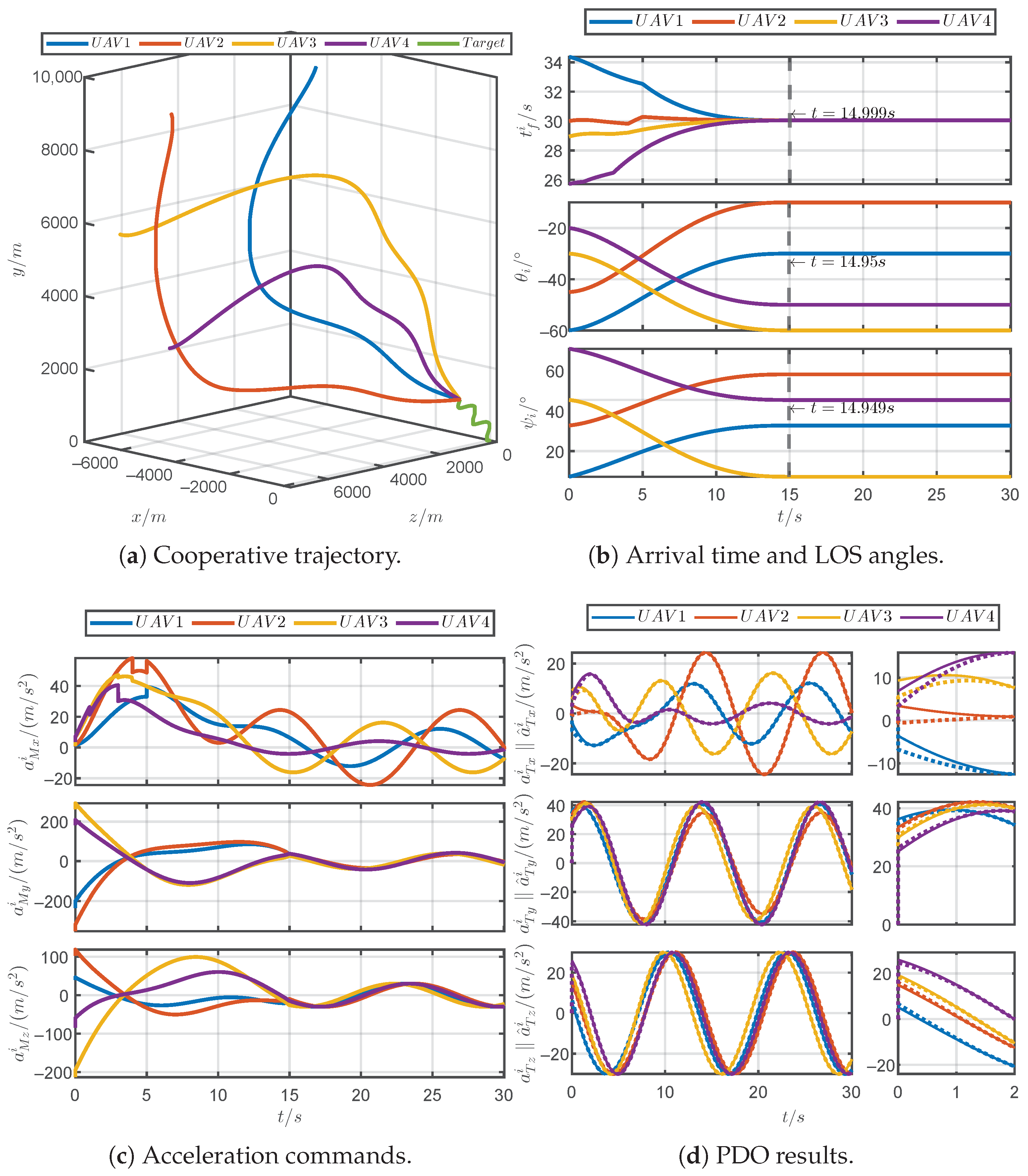
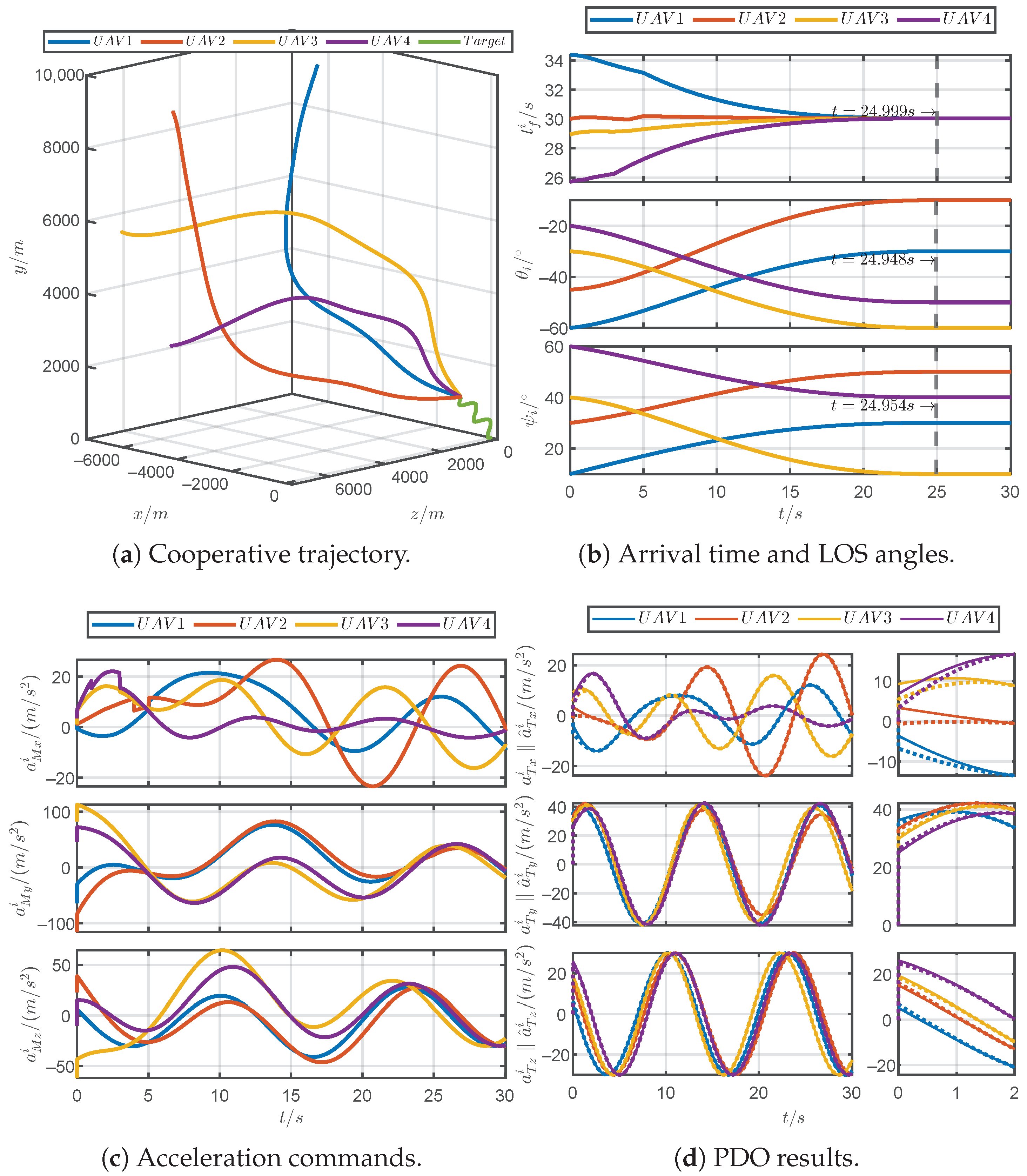
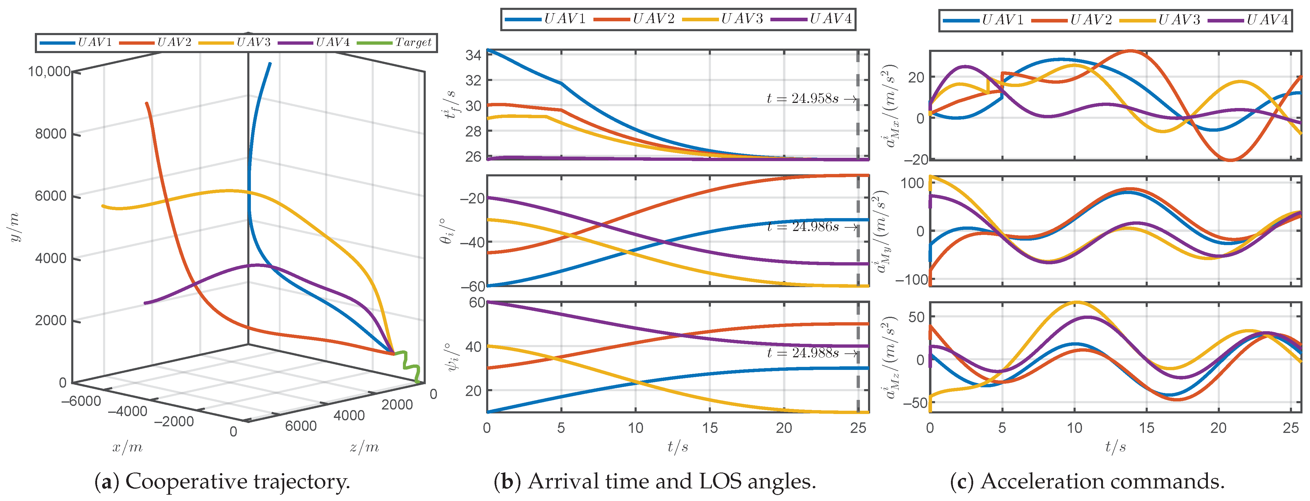
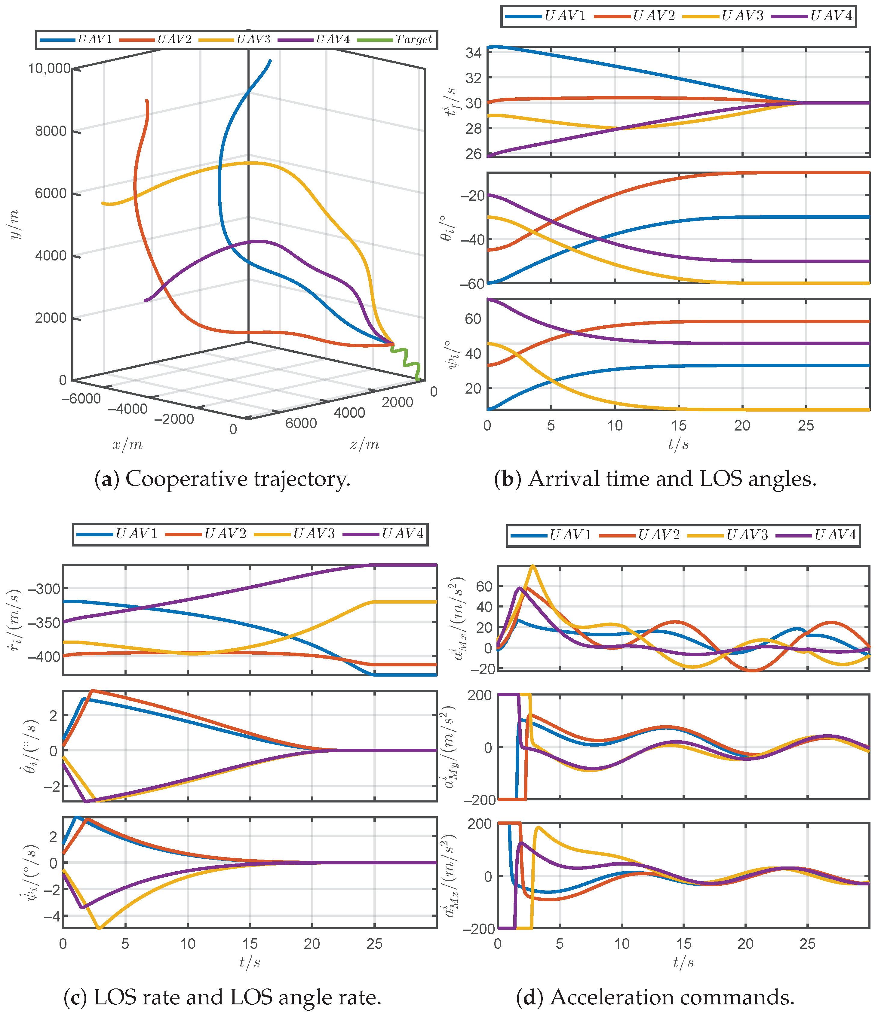
5.1. Simulations for Different Prescribed Settling Times

This subsection will verify the ability of the proposed guidance law to regulate the convergence time. The simulation involves four UAVs cooperatively tracking a dynamic target. The initial conditions and the desired terminal LOS angles of four UAVs are listed in

Table 1. The initial states of the four UAVs.

UAV	UAV 1	UAV 2	UAV 3	UAV 4
$r_i\left(\mathrm{m}\right)$	11,000	12,000	11,000	9000
${\dot{r}}_i(\mathrm{m}/\mathrm{s})$	−320	−400	−380	−350
${\theta }_i{(}^{\circ })$	−60	−45	−30	−20
${\dot{\theta }}_i{(}^{\circ }/\mathrm{s})$	0.630	0.246	−0.355	−0.779
${\theta }_D^i{(}^{\circ })$	−30	−10	−60	−50
${\psi }_i{(}^{\circ })$	10	30	40	60
${\dot{\psi }}_i{(}^{\circ }/\mathrm{s})$	1.404	0.670	−0.521	−0.882
${\psi }_D^i{(}^{\circ })$	30	50	10	40

. The set of the jointly strongly connected topologies is shown in Figure 2. In the inertial coordinate system, the initial position of the target is $\left[0,0,0\right]$ m, the initial velocity is $\left[0,0,100\right]$ m/s, and the acceleration is configured as

$$\left\{\begin{array}{c}{a}_{Tx}=30cos\left(0.5t\right){\mathrm{m}/\mathrm{s}}^2\hfill \\ a_{Ty}=30sin\left(0.5t+\pi /4\right){\mathrm{m}/\mathrm{s}}^2\hfill \\ a_{Tz}=30cos\left(0.5t+\pi /2\right){\mathrm{m}/\mathrm{s}}^2\hfill \end{array}\right..$$

The parameters of PDOs (17), (18), and (19) are chosen as follows: ${\alpha }_o^x={\alpha }_o^y={\alpha }_o^z=0.3$, $b_o^x=b_o^y=b_o^z=1$, ${\kappa }_o^x={\kappa }_o^y={\kappa }_o^z=10$, $T_o^x=T_o^y=T_o^z=2$, ${\varsigma }_o^x={\varsigma }_o^y={\varsigma }_o^z=0.01$, ${\widehat{t}}_f^i\left(0\right)={\widehat{\Theta }}_2^i\left(0\right)={\widehat{\Psi }}_2^i\left(0\right)=0$, and ${\widehat{\xi }}_x^i\left(0\right)={\widehat{\xi }}_y^i\left(0\right)={\widehat{\xi }}_z^i\left(0\right)=0$, ${\widehat{a}}_{Tx}^i\left(0\right)={\widehat{a}}_{Ty}^i\left(0\right)={\widehat{a}}_{Tz}^i\left(0\right)=0$.

The parameters of the accelerations (26), (33), and (35) are listed as follows: ${\alpha }_x={\alpha }_{y1}={\alpha }_{y2}={\alpha }_{z1}={\alpha }_{z2}=0.15$, $b_x=b_{y1}=b_{y2}=b_{z1}=b_{z2}=2$, ${\kappa }_x={\kappa }_{y1}={\kappa }_{y2}={\kappa }_{z1}={\kappa }_{z2}=10$, ${ϵ}_y={ϵ}_z={10}^{-7}$, and $\varrho =0.5$, $T_{y2}=T_{y1}-1$, $T_{z2}=T_{z1}-1$. In order to illustrate that the PRCG law can regulate the convergence time, two different prescribed settling time cases were configured as Case 1: $T_x=T_{y1}=T_{z1}=15$; Case 2: $T_x=T_{y1}=T_{z1}=25$.

Figure 3 shows the network topology switching signals among the UAVs during the simulation. The network topology switching signals in subsequent simulations of this paper are the same as in this figure, unless otherwise noted.

Figure 4 and Figure 5 show the simulation results for Case 1 and Case 2, respectively. From Figure 4a and Figure 5a, it can be seen that the PRCG law can accomplish the cooperative guidance of multiple UAVs to a dynamic target. In Case 1 and Case 2, the maximum miss distances of UAVs were $0.0018$ m and $0.0017$ m, respectively, indicating that high-precision guidance was achieved.

Figure 4b and Figure 5b display the convergence processes of the arrival time and LOS angles. The vertical dashed line indicates the actual convergence time, which is determined by the criteria ${max}_i{t}_f^i\left(t\right)-{min}_i{t}_f^i\left(t\right)<{10}^{-7}s$, ${max}_i\left|{\theta }_i\left(t\right)-{\theta }_D^i\right|<{10}^{-7}\mathrm{rad}$, and ${max}_i\left|{\psi }_i\left(t\right)-{\psi }_D^i\right|<{10}^{-7}\mathrm{rad}$. It can be seen that the arrival times of all UAVs reached consensus within the prescribed time, and the LOS angles converged to the desired values within the prescribed time. The tight alignment between the actual convergence time and the prescribed settling time demonstrates that the PRCG law can accurately preset the settling time.

Figure 4c and Figure 5c show that the acceleration commands of UAVs remain within permissible bounds throughout the guidance process. With the increase in the prescribed settling time, the magnitudes of the acceleration commands are smaller, meaning that less control efforts are required. The acceleration commands are smooth and moderate, except that the early acceleration command $a_{Mx}^i$ jumps due to the network topology switch.

Figure 4d and Figure 5d depict the estimation of target acceleration by PDOs in the LOS coordinate system. The dashed line represents the PDOs’ output and the solid line stands for the true value of the target acceleration. The right-side insets verify that the PDOs completed accurate estimation within the prescribed time. The global plots on the left side illustrate that the PDOs could accurately estimate the target acceleration during the whole guidance.

5.2. Simulations for Different Parameter $\varrho$

This subsection investigates the influence of the parameter $\varrho$ on the cooperative behavior of UAVs. Two extreme cases of the parameter $\varrho$ were considered (Case 3: $\varrho =0$; Case 4: $\varrho =1$). The other parameters remained consistent with those in Case 2.

Figure 6 and Figure 7 present the simulation results for Case 3 and Case 4, respectively. By comparing Figure 6a and Figure 7a, it can be observed that the larger the consensus value of arrival time, the more curved the UAVs’ trajectories became. This is because UAVs need to take detours to increase the arrival time. Figure 6b demonstrates that, when $\varrho =0$, the consensus value of arrival times is the minimum arrival time among UAVs. In contrast, Figure 7b reveals that, when $\varrho =1$, the consensus value of arrival times is the maximum arrival time among UAVs. In Case 3 and Case 4, the maximum miss distances of the UAVs were $0.0020$ m and $0.0013$ m, respectively, indicating that the adjustment of parameter $\varrho$ does not influence the guidance accuracy. Furthermore, it can also be seen that the change in the parameter $\varrho$ did not affect the accuracy of the prescribed settling time or the magnitude of the acceleration command.

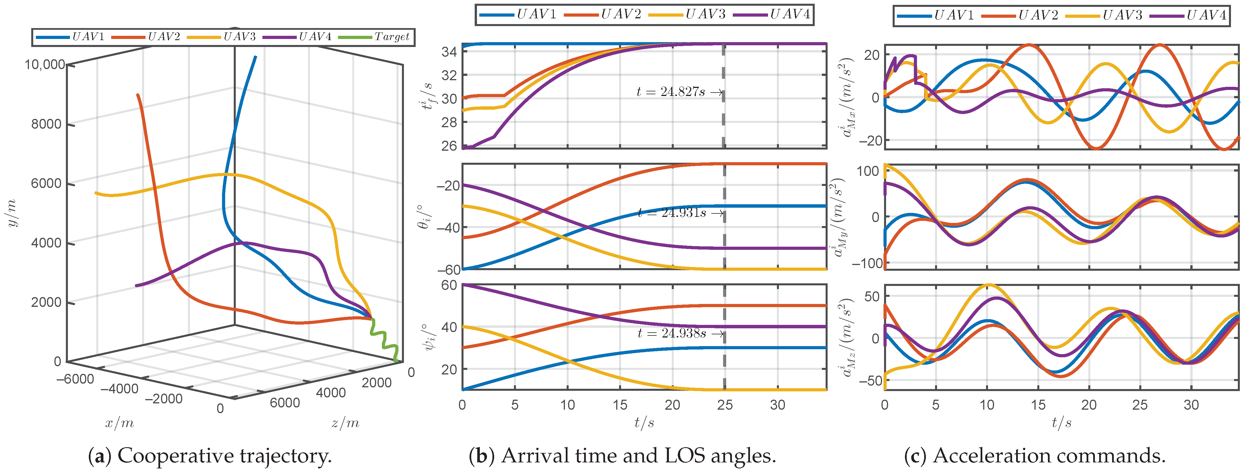
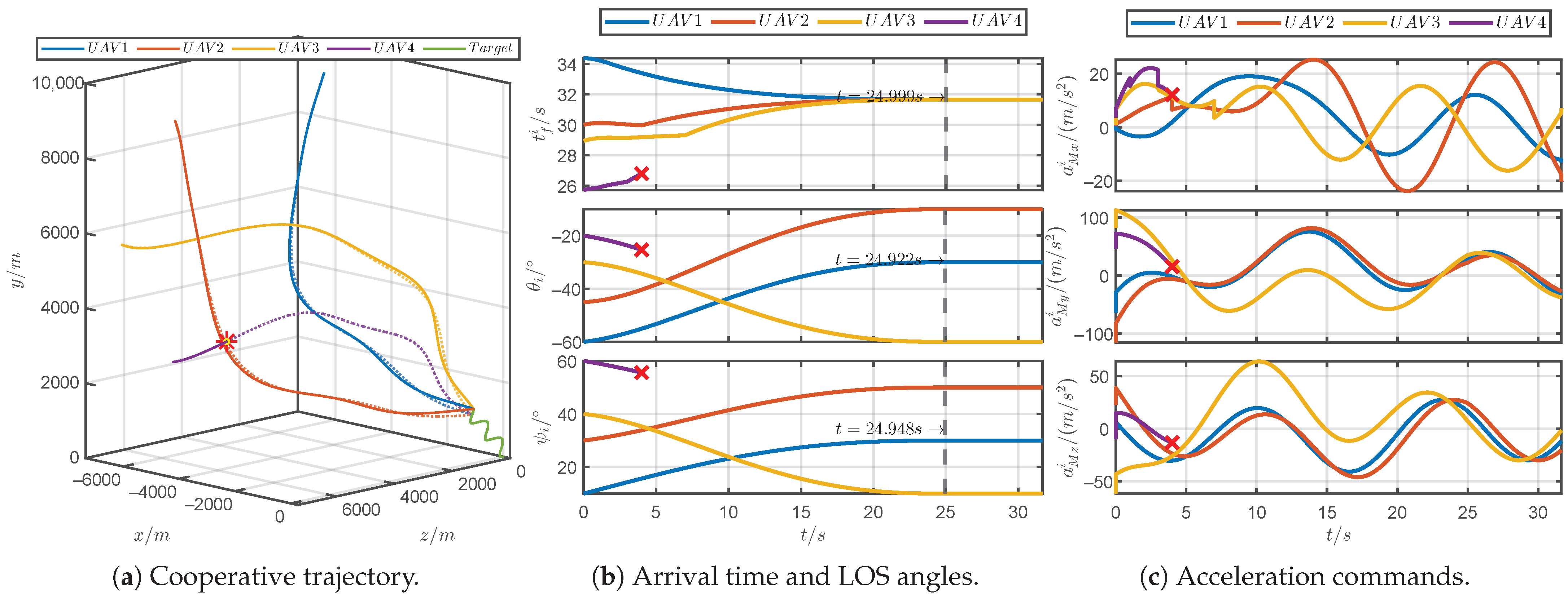
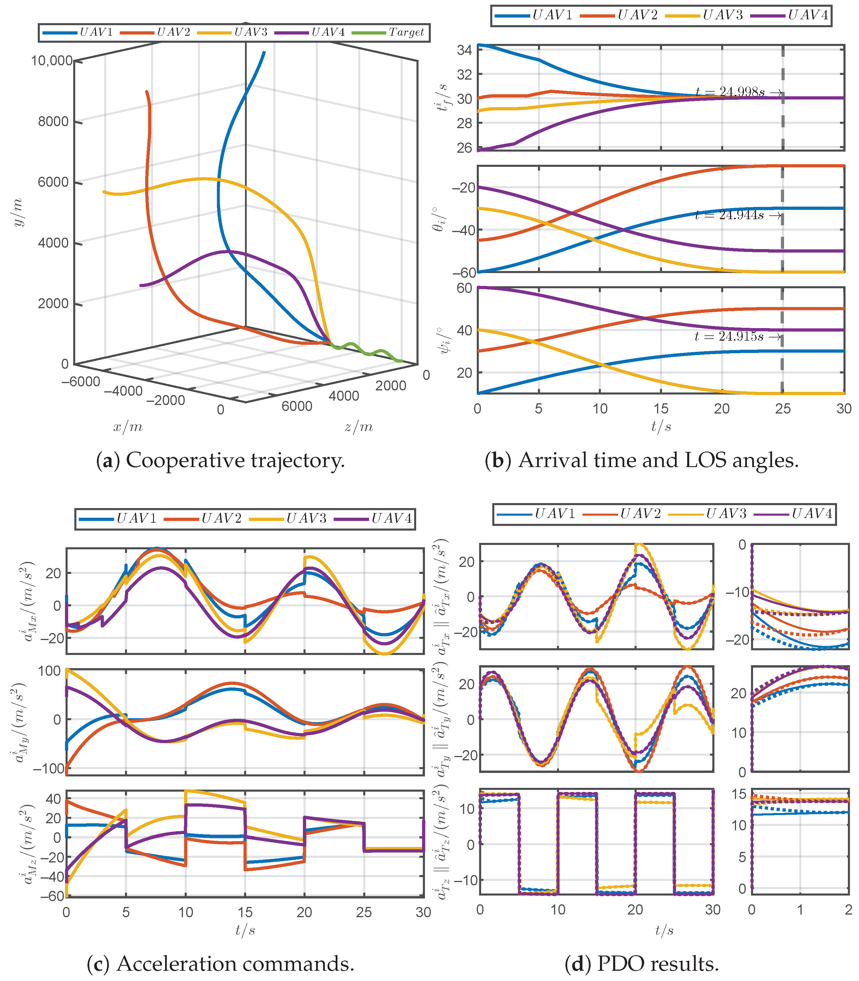
5.3. Simulations for Robustness Verification

This subsection aims to verify the robustness of the PRCG law under the scenario where some UAVs may become faulty. Figure 8 shows the simulation results for the scenario where UAV 4 became faulty at $t=4s$ in Case 2.

In Figure 8a, the dashed line represents the cooperative trajectory without any faulty UAVs, while the solid line represents the cooperative trajectory with the faulty UAV 4. Figure 8a shows that, although UAV 4 became faulty, the surviving UAVs can still achieve cooperative tracking of unknown dynamic targets using the PRCG law. The maximum miss distances of the dashed and solid cooperative trajectories were $0.0018$ m and $0.0019$ m, respectively. This indicates that whether UAVs become faulty or not has no effect on the accuracy of the PRCG law.

A comparative analysis of Figure 5b and Figure 8b revealed two critical observations: Firstly, upon UAV 4 experiencing a malfunction, the remaining UAVs autonomously achieved a new consensus on arrival time, which validates the robustness of the PRCG law. Secondly, regardless of whether some UAVs become faulty or not, the PRCG law can regulate the convergence time accurately.

By comparing Figure 5c and Figure 8c, it can be observed that the disappearance of UAV 4 did not cause any influence on the acceleration commands of the surviving UAVs, which remained smooth and moderate. This is because UAVs perceive the convex hull of the states of neighboring UAVs rather than their real-time states.

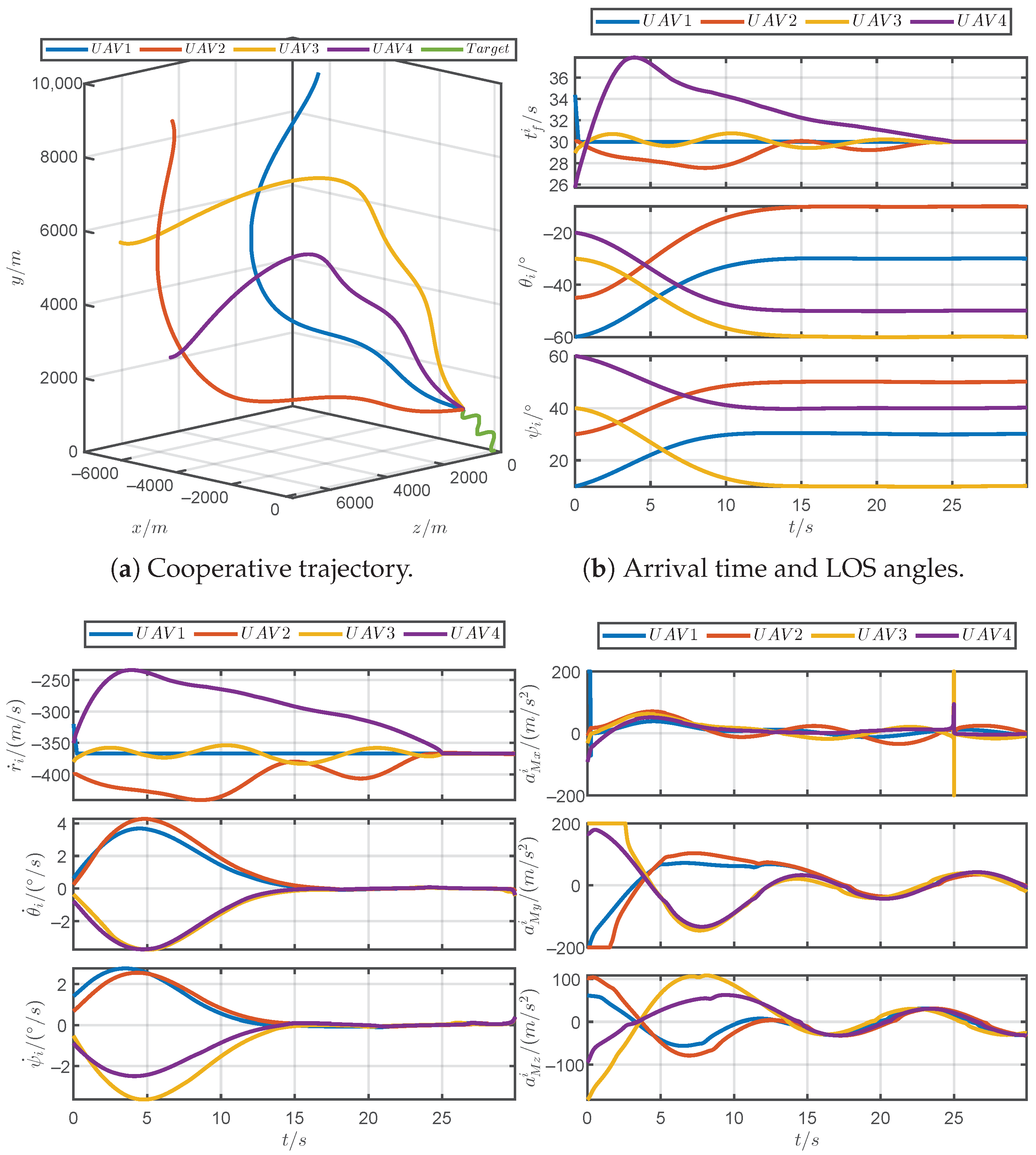
5.4. Simulations for Comparative Verification

Since there is currently no guidance law of the same type that adapts to jointly strongly connected topologies, this subsection will compare the PRCG law with the predefined-time cooperative guidance (PTCG) law in [33] and the appointed-time cooperative guidance (ATCG) law in [36] under a fixed undirected network topology. Figure 9 depicts the network topology among UAVs. In this subsection, the magnitudes of acceleration commands for all guidance laws were limited to $200{\mathrm{m}/\mathrm{s}}^2$. For the PRCG law, except for the network topology, other parameter configurations were the same as those in Case 2.

Detailed information of the PTCG law can be found in [33]. As shown in Figure 9, UAV 1 was designated as the leader for the PTCG law. The desired arrival time of the leader was configured to be 30 s, i.e., $T_d=30$. The prescribed settling time of the PTCG law was configured as 25 s, i.e., $T_r=T_q=T_f=25$. Other parameter configurations were consistent with those in the first subsection of the numerical simulation in [33].

The detailed information of the ATCG law can be found in [36]. To exclude potential unfair influences from different disturbance observers on guidance law performance comparisons, the ATCG law employs the proposed PDOs. The prescribed settling time of the ATCG law is configured as 25 s, i.e., $T_n+T_c=23+2=25$ and $T_f=25$. Other parameter configurations are consistent with those in the first subsection of the numerical simulation in [36].

Figure 10, Figure 11 and Figure 12 show the simulation results of the three guidance laws. From Figure 10a, Figure 11a and Figure 12a, it can be seen that the three guidance laws can perform cooperative tracking of the dynamic target. Figure 10b, Figure 11b and Figure 12b demonstrate that the three guidance laws can satisfy the spatiotemporal constraints within the prescribed time of 25 s. According to the LOS rate and LOS angle rate in Figure 10c, Figure 11c and Figure 12c, the actual convergence time of the PRCG law better matched the prescribed settling time 25 s, indicating that the PRCG law can pre-specify the convergence time more accurately. In Figure 10d, similar to the simulation results in [33], the acceleration command $a_{Mx}^i$ exhibits an abrupt jump at the prescribed settling time 25 s, which is attributed to the infinite gain of the prescribed-time stability method employed by the PTCG law at the prescribed settling time. In addition, compared with Figure 11d and Figure 12d, the acceleration command in Figure 10d is slightly less smooth, which is because the PTCG law employs discontinuous switching sliding mode control to handle the disturbances caused by the dynamic target. In Figure 11d, the initial normal acceleration command is excessively large because the normal acceleration commands of the ATCG law were designed using a predefined-time sliding mode surface. By comparing Figure 10d, Figure 11d and Figure 12d, it can be seen that the acceleration commands of the PRCG law were smoother and more moderate, and they always remained within the limit of $200{\mathrm{m}/\mathrm{s}}^2$.

Table 2. Comparison of the key indicators.

Indicators	PTCG Law	ATCG Law	Ours
Missing distance (m)	$0.0985$	$0.0019$	$0.0018$
Arrival time error (s)	$0.0022$	$1.25\times {10}^{-4}$	$2.00\times 10^{-5}$
Elevation angle error $(°)$	$0.1010$	$5.28\times {10}^{-4}$	$9.13\times 10^{-8}$
Azimuth angle error $(°)$	$0.2417$	$2.36\times {10}^{-4}$	$1.09\times 10^{-7}$
Energy consumption $({\mathrm{m}}^2/{\mathrm{s}}^4)$	$3.05\times {10}^4$	$3.61\times {10}^4$	$9.00\times 10^3$

lists the comparison of the key indicators among the three guidance laws. The miss distance, arrival time error, elevation angle error, and azimuth angle error correspond to the maximum values of these metrics among all UAVs when the UAVs arrive at the target. The energy consumption is calculated as ${\sum }_{i=1}^n{\left(t_f^i\right)}^{-1}{\int }_0^{t_f^i}{\left(a_{Mx}^i\right)}^2+{\left(a_{My}^i\right)}^2+{\left(a_{Mz}^i\right)}^{2}dt$. Firstly, the miss distances of the ATCG law and the PRCG law are similar because the proposed PDOs can accurately compensate for the disturbances caused by the unknown target. Secondly, the arrival time error, elevation angle error, and azimuth angle error of the PRCG law were smaller because the bounded-gain prescribed-time stability criterion does not require sacrificing convergence performance to ensure the boundedness of the gain when implemented. Finally, the energy consumption of the PRCG law was lower, reduced by 70.49% compared with the PTCG law.

In summary, the improvements of the PRCG law compared with the PTCG law and the ATCG law are mainly reflected in three aspects: more accurate prescribed settling time, smaller convergence error, and less control effort. In addition, the PRCG law can adapt to more general network topology.

5.5. Simulations for Unpredictable Maneuvering Target

This subsection will validate the robustness of the proposed guidance law against an unpredictable maneuvering target, wherein a discontinuous maneuvering target is considered. Except for the acceleration of the target, the remaining simulation parameters in this subsection are the same as those in Case 2. In the inertial coordinate system, the acceleration of the target is configured as

$$\left\{\begin{array}{c}{a}_{Tx}=-10\Gamma {\mathrm{m}/\mathrm{s}}^2\hfill \\ a_{Ty}=30sin\left(0.5t+\pi /4\right){\mathrm{m}/\mathrm{s}}^2\hfill \\ a_{Tz}=-10\Gamma {\mathrm{m}/\mathrm{s}}^2\hfill \end{array}\right.,$$

where $\Gamma =1$ if $\mathrm{mod}\left(t,10\right)-5>0$, and $\Gamma =-1$ otherwise.

Figure 13 shows the simulation results of the proposed guidance law for a discontinuous maneuvering target. Figure 13a demonstrates that the PRCG law can guide four UAVs to simultaneously approach the discontinuous maneuvering target. As shown in Figure 13b, it can be observed that the arrival times and the LOS angles can converge within the prescribed time 25 s. As shown in Figure 13c, the acceleration commands for the UAVs consistently remained within the tolerable acceleration limits, and the commands incurred jumps due to the discontinuous maneuvers of the target. Figure 13d reveals that the PDOs could accurately estimate the acceleration of the discontinuous maneuvering target. In brief, the PRCG law can adapt to unpredictable target maneuvers.

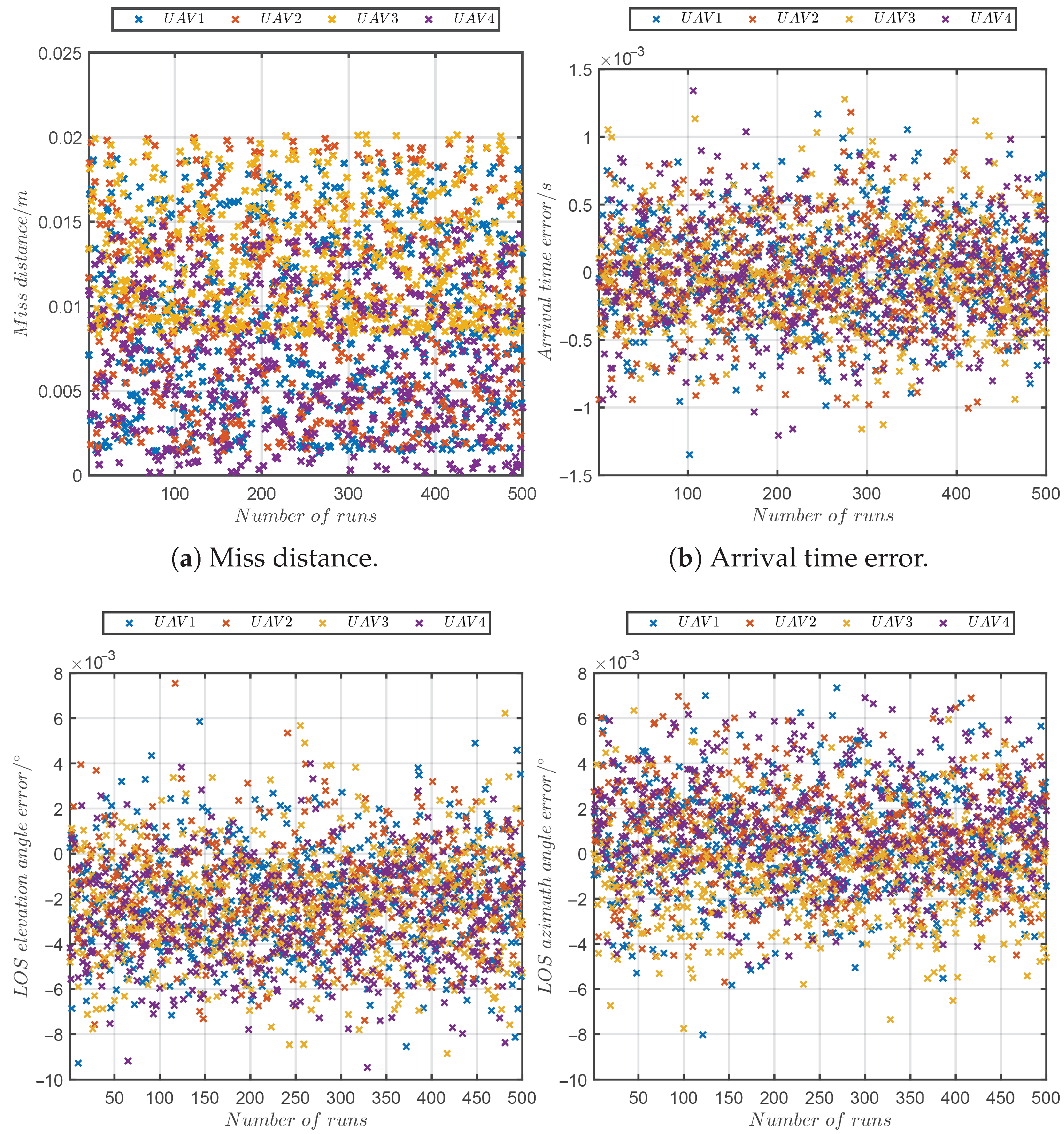
5.6. Monte Carlo Simulation

This subsection will perform Monte Carlo simulation to further validate the robustness of the PRCG law against navigation errors and noises. The initial position errors of the UAVs were configured to follow a uniform distribution over $\left[-100,100\right]$ m, and the initial LOS angle errors were configured to follow a uniform distribution over $\left[-3,3\right]$. The LOS angle measurement noises were configured to follow a zero-mean Gaussian distribution with a standard deviation of $0.2°$. The other parameters remained consistent with those in Case 2. Monte Carlo simulation was performed 500 times under random initial conditions.

Figure 14 shows the Monte Carlo simulation results. It can be found that all of the miss distances kept within $0.0201$ m, all arrival time errors kept within $0.0015$ s, and all LOS elevation angle errors and LOS elevation angle errors kept within $0.01°$. The accuracy displayed above can meet practical requirements. In summary, Monte Carlo simulation demonstrated that the PRCG law is robust to initial errors and measurement noises.

6. Conclusions

This paper proposes a three-dimensional PRCG law, three PDOs, and a novel bounded-gain prescribed-time stability criterion. The PRCG law consists of a tangential acceleration command and normal acceleration commands, and it can guide multiple UAVs with jointly strongly connected topologies to approach a dynamic target simultaneously from specified LOS directions, even if some UAVs become faulty. The tangential acceleration command with a DCHO is proposed to adapt to jointly strongly connected topologies and the contingency of some UAVs being faulty, where the convergence time of arrival times can be specified in advance and the consensus arrival time is a convex combination of the arrival times of all UAVs. Two normal acceleration commands were designed using a prescribed-time nonsingular sliding mode control scheme to regulate the LOS angle error to reach a predetermined neighborhood of zero within a prescribed time. PDOs can accurately estimate the acceleration components of the target without its prior knowledge within a prescribed time. The novel bounded-gain prescribed-time stability criterion ensures boundedness of the time-varying gains in both the guidance law and PDOs without sacrificing convergence performance. Future research directions can focus on two aspects. The first one is the event-triggered spatiotemporal cooperative guidance problem for multiple UAVs subject to jointly strongly connected topologies to further reduce communication burden. The second one is to study the PRCG law when considering communication delays or packet loss.

References

1. Zhan, Y.A.; Li, S.Y.; Zhou, D. Information Fusion-Based Three-Dimensional Two-Stage Optimal Cooperative Predictive Guidance Law. Aerosp. Sci. Technol. 2024, 155, 109533. [Google Scholar] [CrossRef]
2. Wang, C.Y.; Yu, H.S.; Dong, W.; Wang, J.N. Three-Dimensional Impact Angle and Time Control Guidance Law Based on Two-Stage Strategy. IEEE Trans. Aerosp. Electron. Syst. 2022, 58, 5361–5372. [Google Scholar] [CrossRef]
3. Lee, J.I.; Jeon, I.S.; Tahk, M.J. Guidance Law to Control Impact Time and Angle. IEEE Trans. Aerosp. Electron. Syst. 2007, 43, 301–310. [Google Scholar]
4. Liu, Z.Y.; Lei, G.; Xian, Y.; Ren, L.L.; Li, S.P.; Zhang, D.Q. Adaptive Impact-Time-Control Cooperative Guidance Law for UAVs under Time-Varying Velocity Based on Reinforcement Learning. Drones 2025, 9, 262. [Google Scholar] [CrossRef]
5. Dong, W.; Wang, C.Y.; Liu, J.H.; Wang, J.N.; Xin, M. Three-Dimensional Vector Guidance Law with Impact Time and Angle Constraints. J. Frankl. Inst. 2023, 360, 693–718. [Google Scholar] [CrossRef]
6. Dong, W.; Deng, F.; Wang, C.Y.; Wang, J.N.; Xin, M. Three-Dimensional Spatial-Temporal Cooperative Guidance without Active Speed Control. J. Guid. Control. Dyn. 2023, 46, 1981–1996. [Google Scholar] [CrossRef]
7. Li, G.F.; Zuo, Z.Y. Robust Leader-Follower Cooperative Guidance under False-Data Injection Attacks. IEEE Trans. Aerosp. Electron. Syst. 2023, 59, 4511–4524. [Google Scholar] [CrossRef]
8. Wang, C.Y.; Wang, W.L.; Dong, W.; Wang, J.N.; Deng, F. Multiple-Stage Spatial-Temporal Cooperative Guidance without Time-to-Go Estimation. Chin. J. Aeronaut. 2024, 37, S1000936124001900. [Google Scholar] [CrossRef]
9. Liu, T.; Chen, Y.Y.; Li, S. Adaptive Cooperative Estimation and Guidance against Unknown Maneuvering Target. IEEE Trans. Aerosp. Electron. Syst. 2025, 1–12, early access. [Google Scholar] [CrossRef]
10. Cheng, M.; Liu, H.; Xi, J.X.; Zheng, Y.S. Data-Driven Robust Optimal Guidance with Input Saturation via Differential Graphical Game Strategy for Cooperative Aerial Vehicles. IEEE Trans. Intell. Transp. Syst. 2025, 26, 8612–8621. [Google Scholar] [CrossRef]
11. Li, G.F.; Tang, Q.P.; Zuo, Z.Y.; Wu, Y.J.; Lü, J.H. Resilient Cooperative Guidance for Leader-Follower Flight Vehicles against Maneuvering Target. IEEE Trans. Aerosp. Electron. Syst. 2025, 61, 6310–6324. [Google Scholar] [CrossRef]
12. Jiang, Z.J.; Yang, X.X.; Wang, C.; Zhang, Y.; Yu, H. A DMPC-based Three-Dimensional Cooperative Guidance Scheme with Impact Time and Impact Angle Constraints. Meas. Control 2024, 26, 202940241269591. [Google Scholar] [CrossRef]
13. Zhang, S.; Guo, Y.; Liu, Z.G.; Wang, S.C.; Hu, X.X. Finite-Time Cooperative Guidance Strategy for Impact Angle and Time Control. IEEE Trans. Aerosp. Electron. Syst. 2021, 57, 806–819. [Google Scholar] [CrossRef]
14. Zhan, Y.A.; Li, S.Y.; Zhou, D. Time-to-Go Based Three-Dimensional Multi-Missile Spatio-Temporal Cooperative Guidance Law: A Novel Approach for Maneuvering Target Interception. ISA Trans. 2024, 149, 178–195. [Google Scholar] [CrossRef] [PubMed]
15. You, H.; Chang, X.L.; Zhao, J.F.; Wang, S.H.; Zhang, Y.H. Three-Dimensional Impact-Angle-Constrained Cooperative Guidance Strategy against Maneuvering Target. ISA Trans. 2023, 138, 262–280. [Google Scholar] [CrossRef]
16. Yu, H.; Dai, K.R.; Li, H.J.; Zou, Y.; Ma, X.; Ma, S.J.; Zhang, H. Three-Dimensional Adaptive Fixed-Time Cooperative Guidance Law with Impact Time and Angle Constraints. Aerosp. Sci. Technol. 2022, 123, 107450. [Google Scholar] [CrossRef]
17. You, H.; Chang, X.L.; Zhao, J.F.; Wang, S.H.; Zhang, Y.H. Three-Dimensional Impact-Angle-Constrained Fixed-Time Cooperative Guidance Algorithm with Adjustable Impact Time. Aerosp. Sci. Technol. 2023, 141, 108574. [Google Scholar] [CrossRef]
18. Dong, W.; Wang, C.Y.; Wang, J.N.; Zuo, Z.Y.; Shan, J.Y. Fixed-Time Terminal Angle-Constrained Cooperative Guidance Law against Maneuvering Target. IEEE Trans. Aerosp. Electron. Syst. 2022, 58, 1352–1366. [Google Scholar] [CrossRef]
19. Shi, P.F.; Yu, J.L.; Dong, X.W.; Li, Q.D.; Ren, Z. Distributed Adaptive Cooperative Guidance Intercepting Maneuvering Targets with Actuator Faults. IEEE Trans. Aerosp. Electron. Syst. 2024, 60, 5556–5570. [Google Scholar] [CrossRef]
20. Polyakov, A. Nonlinear Feedback Design for Fixed-Time Stabilization of Linear Control Systems. IEEE Trans. Autom. Control 2012, 57, 2106–2110. [Google Scholar] [CrossRef]
21. Sinha, A.; Kumar, S.R. Cooperative Target Capture Using Predefined-Time Consensus over Fixed and Switching Networks. Aerosp. Sci. Technol. 2022, 127, 107686. [Google Scholar] [CrossRef]
22. Chi, H.H.; Ding, X.H.; Zhang, G.L. Three-dimensional cooperative guidance law for multiple missiles with predefined-time convergence. J. Astronaut. 2023, 44, 1238–1250. [Google Scholar]
23. Chang, Y.N.; Wang, X.Z.; Li, G.F. Prescribed-time convergent cooperative guidance method with impact time and angle constraints. J. Beijing Univ. Aeronaut. Astronaut. 2024, 1–14, early access. [Google Scholar] [CrossRef]
24. Zhang, D.; Yu, H.; Dai, K.; Yi, W.; Zhang, H.; Guan, J.; Yuan, S. Three-Dimensional Event-Triggered Predefined-Time Cooperative Guidance Law. Aerospace 2024, 11, 999. [Google Scholar] [CrossRef]
25. Jimenez-Rodriguez, E.; Munoz-Vazquez, A.J.; Sanchez-Torres, J.D.; Defoort, M.; Loukianov, A.G. A Lyapunov-like Characterization of Predefined-Time Stability. IEEE Trans. Autom. Control 2020, 65, 4922–4927. [Google Scholar] [CrossRef]
26. Ning, B.D.; Han, Q.L.; Zuo, Z.Y.; Ding, L.; Lu, Q.; Ge, X.H. Fixed-Time and Prescribed-Time Consensus Control of Multiagent Systems and Its Applications: A Survey of Recent Trends and Methodologies. IEEE Trans. Ind. Inform. 2023, 19, 1121–1135. [Google Scholar] [CrossRef]
27. Song, Y.D.; Wang, Y.J.; Holloway, J.; Krstic, M. Time-Varying Feedback for Regulation of Normal-Form Nonlinear Systems in Prescribed Finite Time. Automatica 2017, 83, 243–251. [Google Scholar] [CrossRef]
28. Ma, W.H.; Fang, Y.W.; Fu, W.X.; Liang, X.G. Three-Dimensional Prescribed-Time Impulsive Pinning Cooperative Guidance. Int. J. Aeronaut. Space Sci. 2023, 24, 1375–1388. [Google Scholar] [CrossRef]
29. Tang, J.C.; Zuo, Z.Y. Cooperative Circular Guidance of Multiple Missiles: A Practical Prescribed-Time Consensus Approach. J. Guid. Control. Dyn. 2023, 46, 1799–1813. [Google Scholar] [CrossRef]
30. Zhang, Y.; Tang, S.J.; Guo, J. Two-Stage Cooperative Guidance Strategy Using a Prescribed-Time Optimal Consensus Method. Aerosp. Sci. Technol. 2020, 100, 105641. [Google Scholar] [CrossRef]
31. Luo, D.H.; Wang, Y.J.; Song, Y.D. Practical Prescribed Time Tracking Control with Bounded Time-Varying Gain under Non-Vanishing Uncertainties. IEEE/CAA J. Autom. Sin. 2024, 11, 219–230. [Google Scholar] [CrossRef]
32. Song, Y.D.; Ye, H.F.; Lewis, F.L. Prescribed-Time Control and Its Latest Developments. IEEE Trans. Syst. Man Cybern. Syst. 2023, 53, 4102–4116. [Google Scholar] [CrossRef]
33. Wang, X.; Cai, Y.L.; Deng, Y.F.; Jiang, H.N. Predefined-Time Spatial-Temporal Cooperative Guidance Law with Leader-Follower Strategy. IEEE Trans. Aerosp. Electron. Syst. 2025, 61, 6053–6069. [Google Scholar] [CrossRef]
34. Wang, Z.K.; Fang, Y.W.; Fu, W.X.; Ma, W.H.; Wang, M.G. Prescribed-Time Cooperative Guidance Law against Manoeuvring Target with Input Saturation. Int. J. Control 2023, 96, 1177–1189. [Google Scholar] [CrossRef]
35. Wang, Z.K.; Fu, W.X.; Fang, Y.W.; Zhu, S.P.; Wu, Z.H.; Wang, M.G. Prescribed-Time Cooperative Guidance Law against Maneuvering Target Based on Leader-Following Strategy. ISA Trans. 2022, 129, 257–270. [Google Scholar] [CrossRef]
36. Zhang, L.; Li, D.Y.; Jing, L.; Ju, X.Z.; Cui, N.G. Appointed-Time Cooperative Guidance Law with Line-of-Sight Angle Constraint and Time-to-Go Control. IEEE Trans. Aerosp. Electron. Syst. 2023, 59, 3142–3155. [Google Scholar] [CrossRef]
37. Holloway, J.; Krstic, M. Prescribed-Time Observers for Linear Systems in Observer Canonical Form. IEEE Trans. Autom. Control 2019, 64, 3905–3912. [Google Scholar] [CrossRef]
38. Ma, W.H.; Guo, X.W. Prescribed-Time Cooperative Guidance Law for Multi-UAV with Intermittent Communication. Drones 2024, 8, 748. [Google Scholar] [CrossRef]
39. Li, Z.H.; Ding, Z.T. Robust Cooperative Guidance Law for Simultaneous Arrival. IEEE Trans. Control Syst. Technol. 2019, 27, 1360–1367. [Google Scholar] [CrossRef]
40. Wang, C.Y.; Ding, X.J.; Wang, J.N.; Shan, J.Y. A Robust Three-Dimensional Cooperative Guidance Law against Maneuvering Target. J. Frankl. Inst. 2020, 357, 5735–5752. [Google Scholar] [CrossRef]
41. Filippov, A.F. Differential Equations with Discontinuous Righthand Sides; Mathematics and Its Applications; Springer: Dordrecht, The Netherlands, 1988; Volume 18. [Google Scholar]
42. Li, C.; Qu, Z. Distributed Finite-Time Consensus of Nonlinear Systems under Switching Topologies. Automatica 2014, 50, 1626–1631. [Google Scholar] [CrossRef]
Figure 1. Three-dimensional UAV–target relative motion geometry.
Drones 09 00474 g001
Figure 2. Jointly strongly connected topologies set.
Drones 09 00474 g002
Figure 3. Network topology switching signals.
Drones 09 00474 g003
Figure 4. Simulation results for Case 1.
Drones 09 00474 g004
Figure 5. Simulation results for Case 2.
Drones 09 00474 g005
Figure 6. Simulation results for Case 3.
Drones 09 00474 g006
Figure 7. Simulation results for Case 4.
Drones 09 00474 g007
Figure 8. Simulation results for robustness verification.
Drones 09 00474 g008
Figure 9. Network topology for comparative verification.
Drones 09 00474 g009
Figure 10. Simulation results for the PTCG law [33].
Drones 09 00474 g010
Figure 11. Simulation results for the ATCG law [36].
Drones 09 00474 g011
Figure 12. Simulation results for the PRCG law.
Drones 09 00474 g012aDrones 09 00474 g012b
Figure 13. Simulation results for the discontinuous maneuvering target.
Drones 09 00474 g013
Figure 14. Monte Carlo simulation results.
Drones 09 00474 g014