Abstract
To overcome the limitations in the perception performance of individual robots and homogeneous robot teams, this paper presents a distributed multi-robot collaborative SLAM method based on air–ground cross-domain cooperation. By integrating environmental perception data from UAV and UGV teams across air and ground domains, this method enables more efficient, robust, and globally consistent autonomous positioning and mapping. First, to address the challenge of significant differences in the field of view between UAVs and UGVs, which complicates achieving a unified environmental understanding, this paper proposes an iterative registration method based on semantic and geometric features assistance. This method calculates the correspondence probability of the air–ground loop closure keyframes using these features and iteratively computes the rotation angle and translation vector to determine the coordinate transformation matrix. The resulting matrix provides strong initialization for back-end optimization, which helps to significantly reduce global pose estimation errors. Next, to overcome the convergence difficulties and high computational complexity of large-scale distributed back-end nonlinear pose graph optimization, this paper introduces a multi-level partitioning majorization–minimization DPGO method incorporating loss kernel optimization. This method constructs a multi-level, balanced pose subgraph based on the coupling degree of robot nodes. Then, it uses the minimization substitution function of non-trivial loss kernel optimization to gradually converge the distributed pose graph optimization problem to a first-order critical point, thereby significantly improving global pose estimation accuracy. Finally, experimental results on benchmark SLAM datasets and the GRACO dataset demonstrate that the proposed method effectively integrates environmental feature information from air–ground cross-domain UAV and UGV teams, achieving high-precision global pose estimation and map construction.
1. Introduction
With the continuous advancement of computer vision and artificial intelligence, robot technology has entered a new stage of rapid development [1,2]. Among these advancements, CSLAM (collaborative simultaneous localization and mapping) has emerged as a core technology for multi-robot cooperative perception and environmental understanding, driving the intelligent evolution of robotics [3,4]. CSLAM tightly integrates environmental perception with multi-robot state estimation, enabling not only high-quality mapping and precise positioning but also improving robots’ adaptability to complex environments [5,6,7]. As a result, robots can operate in broader areas and accomplish more sophisticated tasks. However, while multi-robot collaboration within a single domain has shown great potential, it still faces inherent limitations [8]. To overcome these challenges, air–ground cross-domain collaborative multi-robot SLAM has gained increasing attention as a promising research direction [9,10]. By leveraging the complementary strengths of UAVs and UGVs —such as differences in motion characteristics, load capacity, and communication—this approach significantly expands the application scope of robotic systems, as shown in Figure 1.
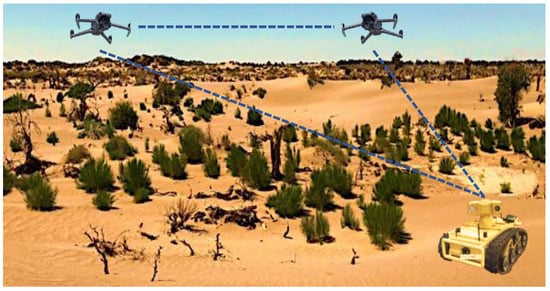
Figure 1.
Air–ground cross-domain collaborative robot team.
In recent years, significant progress has been made in multi-robot collaborative SLAM algorithms. For instance, Rosen et al. [11] introduced SE-Sync, a method that reformulates the multi-robot pose-mapping optimization problem as a maximum likelihood estimation under assumed measurement noise distributions. This enables the recovery of globally optimal solutions for unique Euclidean synchronization. Similarly, Yu et al. [12] developed a Grassmannian manifold map merging algorithm that integrates line and surface features from multiple robots to achieve global map fusion. Building on this, Huang et al. [13] proposed DiSCo-SLAM, which utilizes lightweight descriptors for efficient inter-robot loop closure detection and employs a two-stage distributed Gauss–Seidel method for global pose optimization. Further advancing the field, Lajoie et al. [14] introduced Swarm SLAM, which maximizes algebraic connectivity to select the most critical loop closure keyframes, thereby minimizing communication overhead and enhancing global SLAM accuracy. Additionally, Zhong et al. [15] presented DCL-SLAM, which uses LiDAR–Iris descriptors for efficient loop closure recognition and enables fully distributed collaborative SLAM with interchangeable front-end LiDAR odometry. Despite these advancements, current algorithms still face challenges in air–ground cross-domain collaboration. The extreme disparity in the field of view between UAVs and UGVs makes it difficult to establish consistent environmental feature representations, significantly degrading SLAM accuracy and performance in air–ground multi-robot systems.
To address these limitations, this paper proposes a distributed multi-robot collaborative SLAM method based on air–ground cross-domain cooperation. The algorithm integrates environmental feature information from UAVs and UGVs to achieve global pose estimation and map construction in cross-domain scenarios. Specifically, each robot (UAVs and UGVs) runs a local single-robot semantic-assisted LiDAR odometry module at the front end, capturing real-time local keyframes of its surrounding environment. When UAVs and UGVs come within communication range, they exchange keyframe feature information and perform PCM (pairwise consistency maximization) incremental anomaly detection [16] to eliminate erroneous inter-robot loop closures. After validating loop closure candidates, the algorithm employs an iterative registration method based on semantic and geometric features assistance to compute the coordinate transformation matrix between UAVs and UGVs’ point clouds. This establishes a unified coordinate system and provides robust initialization for backend optimization. Finally, the method implements a multi-level partitioning majorization–minimization DPGO method incorporating loss kernel optimization. This approach decouples factor graphs from different robot nodes, performing majorization–minimization with loss kernel optimization to ensure gentle convergence to first-order critical points. The high-precision positioning and map construction of the global robot are realized. The main contributions of this paper are as follows:
- To address the significant field-of-view disparity and alignment errors between UAVs and UGVs, we propose an iterative registration method based on semantic and geometric features assistance. The method uses semantic and geometric features to calculate the corresponding probability of loop closures. Then, through iterative optimization of rotation angles and translation vectors, our approach computes the optimal coordinate transformation matrix, ensuring all robots operate in a unified coordinate system during backend optimization. This effectively reduces pose estimation errors in cross-domain collaboration.
- To address the challenges in large-scale nonlinear DPGO, including convergence difficulties and high computational complexity, we propose a multi-level partitioning majorization–minimization DPGO method incorporating loss kernel optimization. Our method constructs multi-level balanced subgraphs based on node coupling degrees. Our method formulates a non-trivial loss kernel optimization framework using majorization–minimization surrogate functions, enabling DPGO to converge smoothly to first-order critical points while significantly improving positioning and pose estimation accuracy.
- Extensive experiments are conducted to evaluate the effectiveness of the proposed method. The experimental results show that the proposed method can effectively integrate the environment feature information of the air–ground cross-domain UAV and UGV teams and cooperate to achieve high-precision global pose estimation and map construction.
2. Related Work
In this section, we will briefly introduce existing research methods on distributed pose graph optimization and air–ground cross-domain cooperative SLAM.
2.1. Distributed Pose Graph Optimization
Choudhary et al. [17] first proposed the distributed Gauss–Seidel (DGS) algorithm, which approximates the maximum likelihood trajectory estimation problem by decoupling it into two sequential subproblems of rotation and translation components, resolved through a two-phase distributed DGS framework. During distributed iterations, each robot employs quadratic relaxation and projection for rotation initialization to eliminate non-convex constraints, followed by single-iteration Gauss–Newton refinement to recover complete poses, ultimately converging to centralized pose estimation benchmarks. Tian et al. [18] introduced an asynchronous stochastic parallel PGO method operable without synchronization. Through Riemannian gradient optimization with bounded time-delay rank relaxation, they established global first-order convergence with sufficiently small step sizes. Inspired by SE-Sync [11], they further proposed a verifiable distributed PGO method via Riemannian block coordinate descent, proving convergence to global first-order critical points under specified conditions—representing the first asynchronous algorithm for multi-robot SLAM applications.
Recent work by Tian et al. [19] enhanced the distributed PGO with robust kernel improvements using graduated non-convexity (GNC) [20] to estimate inter-frame transformations, initializing local trajectories in global coordinates. They formulated a progressively non-convex Riemannian block coordinate descent method to resolve distributed PGO optimization. Fan et al. [21] developed a majorization–minimization (MM) method for distributed PGO, ensuring convergence to first-order critical points. Unlike previous approaches representing each pose as individual nodes, their method updates all poses from the same robot as unified nodes, utilizing enhanced constraint information. They implemented an accelerated initialization approach with quadratic convergence properties for distributed PGO and redesigned the optimization using Nesterov [22] acceleration, significantly improving computational efficiency while reducing inter-node communication redundancy. Li et al. [23] proposed a multi-level graph-distributed PGO algorithm combining graph partitioning with Riemannian optimization. Their approach refines highly coupled nodes through multi-level graph partitioning, reformulates distributed PGO as low-rank convex relaxation, and solves it via modified Riemannian block coordinate descent.
2.2. Air–Ground Cross-Domain Cooperative SLAM
He et al. [24] proposed a camera–LiDAR fusion method for multi-robot collaborative SLAM. Their framework incorporates a visual–LiDAR odometry module with point-line-plane constraints to provide robust front-end odometry. The system generates thumbnail representations delineating obstacle contours, employs neural networks for descriptor extraction to facilitate inter-robot data association, and ultimately integrates map segments with robot poses to achieve superior cross-domain collaborative localization and mapping. Zhong et al. [15] devised DCL-SLAM, a front-end replaceable fully distributed SLAM framework for multi-robot collaboration in unknown environments. Operating through peer-to-peer communication, the system utilizes lightweight LiDAR–Iris descriptors for inter-robot place recognition and rejects spurious inter-robot loop closures via PCM-based maximal clique set verification.
Liu et al. [25] innovatively developed a bio-inspired semantic SLAM framework for large-scale heterogeneous cross-domain collaboration. Their approach constructs semi-dense semantic maps through bio-inspired tightly-coupled visual-inertial odometry, employing neural-inspired compact encoding for biological motion cues. The topological data of semantic features serve as cross-view scene descriptors, enabling air–ground heterogeneous robots to recognize identical scenes under viewpoint variations, thereby accomplishing large-scale environmental mapping. Duan et al. [26] created a ground-prior-assisted localization method for air–ground heterogeneous robots. The approach first generates rotation-invariant candidate co-visualization context descriptors using pre-mapped ground references, establishing unified representation for heterogeneous point cloud features. Heterogeneous robots then achieve refined positioning through descriptor matching between queried co-visual contexts and allocated candidate descriptors. Qiao et al. [27] introduced a genetic algorithm-based cross-domain semantic map registration method for significant viewpoint variations. This technique employs a fitness evaluation model combining semantic–geometric feature correlations, implements latent semantic correspondence selection to eliminate outliers, and incorporates an adaptive mutation step-size adjustment strategy to accelerate convergence while enhancing co-location precision.
3. Materials and Methods
Figure 2 demonstrates the architectural framework of the distributed multi-robot collaborative SLAM method based on air–ground cross-domain cooperation. The framework achieves environmental perception and global optimization through a coordinated mechanism integrating three modules, namely the robot-local front-end module, the distributed loop closure configuration module, and the robust DPGO back-end module. In the robot-local front-end module, both UGVs and UAVs employ SA-LIO [28] methodology to process raw LiDAR–IMU measurements, producing real-time local odometer trajectories while extracting semantic-assisted loop closure keyframes. The next step involves establishing good communication between robots. The distributed loop closure configuration module begins by utilizing the PCM incremental anomaly detection module to filter out erroneous loop closure detection keyframes that may arise from interactions between different robots. Only valid loop closure keyframes are retained for further processing. Next, an iterative registration method based on semantic and geometric features assistance calculates the precise transformation matrix between the corresponding valid loop closure detection keyframes. This process provides a reliable initialization for relative pose measurement used in the back-end DPGO. Finally, the robust DPGO back-end module constructs a multi-level balanced optimization subgraph based on the degree of coupling between the relative pose measurements of robot nodes. It constructs a majorization–minimization substitute function for nontrivial loss kernel optimization to integrate and optimize intra-robot local pose estimations and inter-robot relative pose, thereby achieving globally optimal trajectory estimation and high-precision map construction. The technical implementations of these modules will be comprehensively discussed in the following sections.
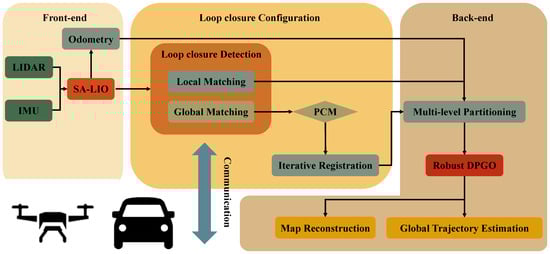
Figure 2.
The architectural framework of the air–ground cross-domain collaborative SLAM system.
3.1. Robot-Local Front-End Module
Both UGVs and UAVs autonomously implement the SA-LIO [28] algorithm locally. This enables them to generate real-time local motion trajectories by fusing LiDAR and IMU data. The process also constructs semantic-enhanced local point cloud keyframes for loop closure detection. The algorithm effectively filters out dynamic objects and conducts precise semantic segmentation of static environments by processing point cloud data using a deep learning-based neural network. Laser odometry is utilized for real-time local pose estimation. Additionally, the semantic features extracted from the keyframes are employed to identify candidates for loop closure, which facilitates distributed loop closure detection for air–ground cross-domain teams of UAVs and UGVs. For a detailed introduction to the SA-LIO algorithm, please refer to reference [28]; further explanation is not provided here.
3.2. Distributed Loop Closure Configuration Module
When UAVs and UGVs enter the communication range, they exchange local loop closure keyframe information. To address the challenges of erroneous loop closure detection and the significant field-of-view disparity between UAVs and UGVs, the paper proposes a distributed loop closure configuration module. This module consists of the following two key components: (1) A PCM [16] incremental anomaly detection module that filters out incorrect inter-robot loop closures, and (2) an iterative registration method based on semantic and geometric features assistance that computes transformation matrices between corresponding air–ground keyframes, providing well-initialized, unified coordinate references for subsequent DPGO.
3.2.1. PCM Incremental Anomaly Detection Module
When two robots enter each other’s communication range, they exchange local loop closure detection keyframes. However, significant differences in the field of view between UAVs and UGVs, as well as inaccuracies in loop closure detection due to repetitive scenes, can severely impact subsequent global pose optimization. To eliminate errors in keyframes during the air–ground loop closure detection, we utilize the PCM [16] incremental anomaly detection module. The PCM incremental anomaly detection module verifies the accuracy of loop closure detection by examining the consistency of inter-robot noise measurements.
Consider a multi-robot system comprising robots, where each robot only possesses local perception capabilities. Each robot includes a set of poses denoted as , where represents the special Euclidean group in d-dimensional space. A pose can be decomposed into a rotation matrix and a translation vector , with denoting the special orthogonal group. The intra-robot noisy measurements are expressed as . Similarly, the inter-robot noisy measurements are defined as , where denote distinct robots. Here, represent translational measurements, while correspond to rotational measurements. These measurements adhere to the following noise model:
where denotes the identity matrix. The isotropic Langevin noise model for rotational components serves as the directional counterpart to Gaussian noise applied in translational components.
The loop closure is deemed acceptable when the measurement noise between two robots satisfies the following condition:
where and denote intra-robot noisy measurements between keyframes and for robot , and between keyframes and for robot , respectively. On the other hand, the terms and represent inter-robot noisy measurements: refers to the measurement between robot at keyframe and robot at keyframe , while corresponds to the measurement between robot at keyframe and robot at keyframe . Finally, the threshold parameter is empirically set to in our system configuration.
We utilized the PCM incremental anomaly detection module to filter out erroneous loop closure detection keyframes that occurred due to interactions between different robots. Only the valid loop closure keyframes were retained for further processing, which ultimately improved the accuracy and robustness of the subsequent optimization process.
3.2.2. Iterative Registration Method Based on Semantic and Geometric Features Assistance
After identifying the correct loop closure detection keyframes between the UAVs and UGVs, the next step is to accurately determine the relative pose measurements. This step is essential for eliminating optimization errors that arise from the significant differences in field-of-view between the UAVs and UGVs. For the local loop closure semantic keyframes and , provided by the UAV and UGV, respectively, we aim to find a transformation matrix . This matrix, which consists of a rotation matrix and a translation vector , seeks to minimize the coordinate transformation error in the point cloud mapping between the UAV and UGV. However, directly determining the transformation matrix between the heterogeneous coordinate systems of the UAV and UGV is a highly challenging task [29].
To achieve precise global coordinate transformation, we recast the problem of minimizing coordinate transformation error as a probabilistic correspondence problem in heterogeneous point cloud alignment. Specifically, the higher the probability of the corresponding point in the local ring closed mapping, the smaller the error of the correlation coordinate transformation, and the higher the precision of the transformation matrix [27]. Consequently, we propose an iterative registration method based on semantic and geometric feature assistance. The method structure is shown in Figure 3, which integrates semantic and geometric descriptors. It is followed by an iterative optimization scheme to determine the loop closure transformation matrix through successive refinements of and .
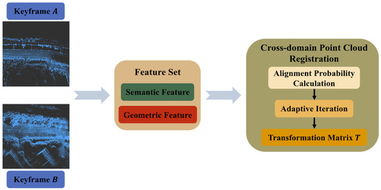
Figure 3.
The structure of the iterative registration method based on semantic and geometric feature assistance.
Based on line and surface features descriptors extracted from UAV and UGV heterogeneous robots’ keyframes, we derive the key feature point set in local point cloud map . For each key feature point , its surrounding semantic distribution is characterized as , where represents the semantic labels of neighboring points. These points are clustered into groups where all points within each group share identical semantic labels. Let and denote the geometric coordinate and semantic label of the -th feature point in , respectively, where . Assuming the transformed counterpart of in the loop closure candidate map is , with and representing corresponding geometric coordinates and semantic labels, a higher correspondence probability between and in global coordinates enhances the accuracy of the transformation matrix , thereby reducing alignment errors. The formula for calculating the probability of potential corresponding points is as follows:
where represents the semantic similarity measure between keypoint and its potential correspondence . The value is 1 if and only if and have the same semantic feature label, and 0 in other cases. Equation (5) is as follows:
quantifies the geometric similarity measure between keypoint and its potential correspondence . The correspondence probability under transformation matrix is computed using a Gaussian probability density function, formally expressed as follows:
where denotes the transformation function associated with the current transformation matrix , and represents the covariance matrix of geometric feature residuals, computed as follows:
where denotes the rotation matrix component, and and represent the geometric feature covariance matrices associated with potential corresponding points and , respectively.
This leads to the derivation of the correspondence probability formulation for the UAV and UGV teams’ local maps and under transformation matrix , as follows:
The optimal transformation matrix is subsequently computed via an adaptive iterative adjustment strategy, as outlined in Algorithm 1. First, the initial parameters are given, namely rotation matrix , translation vector , and predefined threshold . The algorithm then iteratively evaluates the correspondence probability using the current transformation parameters, compares the result with , and adaptively adjusts the rotation angles and translation step sizes. Through continuous iteration, the optimal cross-domain coordinate transformation matrix between UAV and UGV is ultimately determined. This process provides reliable relative pose measurement initialization for the back-end DPGO.
| Algorithm 1. Adaptive Iterative Adjustment Strategy |
| Input: Initial rotation Angle Initial translation vector Threshold of the probability corresponding |
| Output: Rotation angle Translation vector |
| Function |
| while (True) do evaluate fusing Equation (8) |
| if () then |
| else if () then |
| else if () then |
| else |
| end if |
| end while |
| return |
| End |
3.3. Robust DPGO Back-End Module
After passing through the distributed loop closure configuration module, effective pose initialization was achieved among multiple UAVs and UGVs in the air–ground cross-domain. The next step is to perform pose estimation and optimization of the global robot using the robust DPGO back-end module. To enhance the robustness and accuracy of the DPGO in the proposed method and to mitigate the negative effects caused by false loop closures, this paper introduces a multi-level partitioning majorization–minimization DPGO method incorporating loss kernel optimization.
DPGO, as a nonlinear non-convex optimization problem, estimates unknown poses by modeling multi-robot trajectories as graph structures where vertices represent individual poses and edges represent relative pose constraints [30]. DPGO in the proposed method integrates mileage estimation within robots and loop closure constraints between robots to collaboratively solve globally consistent trajectories among air–ground cross-domain UAVs and UGVs [31]. The DPGO problem is formally modeled through a directed graph , where the vertex represents unknown poses of robot at keyframe , and the directed edge represents noisy relative measurements between robot at keyframe and robot at keyframe . The directed graph is assumed to exhibit weak connectivity, which ensures the solvability of the optimization problem while maintaining algorithmic generality.
The directed graph represents an idealized model under the assumption of perfect loop closure detection. In practical multi-robot systems, however, inter-robot measurements are susceptible to outliers caused by erroneous loop closures, which introduce significant noise in relative pose estimation and degrade DPGO performance [32]. To address these measurement anomalies and improve the optimization accuracy, we construct a robust multi-level graph-optimized DPGO problem with Huber loss function through maximum likelihood estimation, as follows:
The objective function is defined as follows:
where denote the weights of each part of the noisy measurements, respectively. represents Huber nontrivial loss kernel, which is specifically defined as follows:
where . The Huber nontrivial loss kernel function is shown in Figure 4.
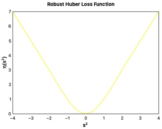
Figure 4.
Huber loss kernel.
To enhance communication efficiency, reduce communication overhead, and improve optimization performance for DPGO, we adopt a multi-level partitioning strategy for the directed graph . The original multi-robot pose graph is recursively decomposed into balanced subgraphs across multiple hierarchical levels.
As shown in Figure 5, the procedure begins by partitioning into -balanced subgraphs using edge-cut or vertex-cut methods, with the choice between these strategies depending on the graph’s inherent connectivity patterns [33]. Subsequently, each subgraph is further partitioned to generate disjoint node sets . Notably, the state space of every robot node combines both its local pose information and pose estimates from adjacent robots within the same hierarchical level. Specific definitions are as follows:
where represents all the poses contained in each subgraph after subgraph division. The following multi-level partitioning DPGO problem can be formulated as follows:
where Equations (15)–(17) are as follows:
where denotes the multi-level partitioning DPGO subproblem constructed for robot , and represents the constraint set from local pose edges associated with robot .
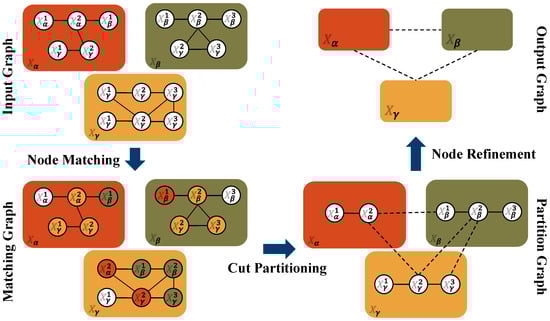
Figure 5.
Procedure of the multi-level graph partitioning.
For a simpler representation, the above formula can be rewritten as follows:
where and represent the measurement estimates within and between nodes of robot , respectively. Equations (19) and (20) are as follows:
Next, we can achieve global optimization of DPGO by optimizing each component of the objective function.
According to reference [31], when or , there exists a sparse positive semidefinite matrix that satisfies the following Equation (21):
Then, the forms of the measurement in the robot node and the measurement between nodes can be expressed as follows:
For any matrix , it can be easily proved that the following is true:
where is a positive semidefinite, and the equation holds when . If , the above formula can be rewritten as follows:
Applying the above formula to the right side of yields the following:
At the same time, due to , it can be further expressed as follows:
There is a positive semidefinite matrix such that the right side of the above equation can be rewritten as follows:
where is a block diagonal matrix that can be used to decouple the unknown poses of different nodes.
Let , where represents the iteration state variable of . So, for any , the minimized agent function of can be obtained as follows:
The equation holds when . Here, is the weight associated with the loss kernel function, defined as follows:
So, the agent function of can be further constructed, for any can obtain the following:
where . Furthermore, the equation holds when .
We can further obtain the following:
The equation holds when .
There also exists a positive semidefinite matrix such that Equation (33) is as follows:
where represents the Euclidean gradient of with respect to at .
For any node , is equivalent to the following:
where is a function of a single pose ; represents the -th position in the directed graph of node . Furthermore, there exists a positive semidefinite matrix such that Equation (35) is as follows:
where represents the Euclidean gradient of at with respect to a single pose .
couples multi-level directed graphs of different nodes, enabling the majorization–minimization methods of DPGO to be possible. By setting and letting it approach 0 so that becomes the tightest upper bound surrogate function of , the convergence speed and convergence stability are improved.
Therefore, the optimization problem of can be solved by solving the independent optimization problem of in a single node . Based on the above formula derivation, the following update rules are proposed:
Since Equations (34) and (36) can be solved in a single multi-level partitioned node , we can further decompose Equation (36) into an independent optimization problem for a single pose at the node , as follows:
According to the above equation, Equation (38) is as follows:
The above derivation shows that . Therefore, Equations (36) and (37) above are reasonable update rules for distributed PGO. These rules have proven convergence for first-order critical points. The specific optimization algorithm formulated according to the optimization rules is shown in Algorithm 2. The algorithm details are as follows:
- (1)
- In the sixth row of Algorithm 2, each robot node performs a round of inter-node communication to obtain from its neighbor robot node ;
- (2)
- In the seventh row of Algorithm 2, each robot node using its state with its neighbors evaluates , ;
- (3)
- In rows 8 to 11 of Algorithm 2, is calculated for each robot node ;
- (4)
- In row 11 of Algorithm 2, each robot node is iteratively optimized to improve the final solution .
| Algorithm 2. Multi-level Partitioning DPGO Method |
| Input: An initial iterate and . |
| Output: A sequence of iterates Function |
| for do |
| for node do |
| retrieve from |
| evaluate , |
| for do |
| retrieve from in which |
| end for |
| retrieve from in which |
| end for |
| end for |
| return end |
The proposed optimization algorithm requires no extra computational effort, as long as each robot node communicates with its neighbor robot node . Next, the first-order convergence of the algorithm will be verified.
Theorem 1.
Suppose that for any node , the following conditions hold:
where denotes the Riemannian gradient. Then, for the iterative sequence generated by the optimization algorithm, we can conclude the following:
- (1)
- is a non-increasing function.
- (2)
- as .
- (3)
- as , if .
- (4)
- as , if .
Proof:
- (1)
- According to Formulas (31) and (32), we can deduce the following:This equation holds when . From Formula (38), we can derive the following conclusions:Therefore, we can prove that (1) holds, and that is a non-increasing function.
- (2)
- Since (1) holds and , we can conclude the following:
- (3)
- According to Formula (42), we have the following:Substituting Formulas (29) and (33) into the above equation, we obtain the following:Since , we can derive the following:where is a constant scalar. As , we have , and, thus, when , . Therefore, we can conclude the following:
- (4)
- Since (3) holds true and is continuous, it follows that as , if . □
Thus, we can demonstrate that the DPGO method presented in this paper converges gently. Compared with other DPGO methods, the multi-level partitioning DPGO method incorporating loss kernel optimization proposed in this paper has the most relaxed first-order convergence requirements, while significantly enhancing the convergence performance of nonlinear optimization.
The above DPGO method operates periodically on each robot. Each robot first determines neighboring robots within communication range by analyzing connectivity in the distributed pose factor graph. Subsequently, it performs loop closure detection through interactive keyframe matching. Following the elimination of erroneous keyframes and computation of the optimal loop closure transformation matrix, the method implements the multi-level partitioning majorization–minimization DPGO method incorporating loss kernel optimization. In each iteration of the algorithm, the optimal solution for each robot pose estimation is found, and a consensus is reached on the optimal trajectory and pose estimation.
4. Results
This section presents a systematic evaluation of the performance of the distributed multi-robot collaborative SLAM method based on air–ground cross-domain cooperation proposed in this paper. First, we conduct numerical experiments comparing our DPGO optimization approach with existing methods, specifically analyzing its convergence speed and optimization accuracy. Second, we validate the method’s practical performance in air–ground cooperative UAV and UGV teams by assessing trajectory estimation accuracy and map construction quality using air–ground multi-robot datasets. Experimental results demonstrate that our method offers significant advantages for air–ground cooperative UAV and UGV teams, delivering robust, high-precision pose and trajectory estimation while maintaining global map consistency.
4.1. DPGO Performance Analysis
We evaluate our DPGO method using 2D and 3D SLAM standard benchmark datasets. The 3D evaluation employs standard datasets including the Sphere, Grid, Garage, and Torus, while the 2D evaluation utilizes the City and CSAIL datasets [11]. This dual-testing framework guarantees a reliable assessment of the method’s universality and practical applicability across different scenarios.
We employ two quantitative metrics to evaluate method performance: the relative suboptimality gap and the Riemannian gradient norm [21].
The relative suboptimality gap is defined as , Where denotes the objective value at each iteration and represents the global optimal value computed by SE-SYNC [11]. Specifically, SE-SYNC reformulates the original pose graph’s non-convex optimization problem as follows through semi-definite relaxation and Riemannian optimization on matrix manifolds:
where is the coefficient matrix constructed by the noise measured values, defined as follows:
where and represent the intra-robot measurement noise, the inter-robot measurement noise, and the anchor point constraints, respectively. These covariance matrices are explicitly defined as follows:
where and represent the rotation information matrix and the translation information matrix, respectively. represents the anchor point pose set of robot a, while corresponds to the standard basis vector.
In Equation (50), represents the matrix variable of the rotation vector relaxed by SDP and is defined as follows:
where is the rotation vector remapped to its corresponding rotation matrix via . After computing the global optimal objective value , the relative suboptimal gap at each iteration is quantified. Convergence to the global optimum is indicated as this value approaches zero.
The Riemannian gradient norm measures the variations of the gradient during optimization. Its global measure is defined as follows:
where represents the product manifold of the rotational group. The term denotes the Riemannian gradient associated with a single robot, specifically defined as follows:
where is a function of the projection form of Lie algebra. The smaller the global Riemannian gradient norm, the stronger the convergence it indicates.
These complementary metrics comprehensively evaluate the convergence performance of the method from different angles and provide a comprehensive quantitative basis for the optimization effect.
To rigorously evaluate our proposed DPGO optimization method, we conduct comparative experiments with three state-of-the-art PGO algorithms, including DGS (distributed Gauss–Seidel) [17], RCBD++ (accelerated Riemannian block coordinate descent) [18], and MM-PGO (majorization–minimization methods for distributed pose graph optimization) [21]. Among them, DGS adopts the standard configuration, while RCBD++ and MM-PGO are configured based on the Nesterov acceleration algorithm. For comprehensive scalability validation, we test all methods using 5-node and 10-node robot team configurations. The comparative results are presented in Table 1.

Table 1.
Results of DPGO data on 2D and 3D baseline datasets for each method.
The scalar in Table 1 denotes the globally optimized objective value for the multi-robot pose graph optimization problem, which corresponds to the negative log-likelihood under the given measurement noise model. Its magnitude is determined by the covariance-weighted sum of all measurement residuals (rotational and translational), inherently lacking a unified dimension. We typically focus more on the numerical change relative to the initial value than on its physical unit. However, this value can serve as an indicator of the pose graph’s consistency. A smaller value indicates a higher consistency in the pose graph.
Table 1 presents the objective function values of each method at 12, 25, 50, 100, 250, and 500 iterations for both 5-node and 10-node robot systems. The key advantage of DPGO is its ability to achieve higher precision more quickly, rather than its eventual attainment of the highest possible precision. The results highlight the correlation between convergence rate and iteration count across various optimization methods. These data demonstrate the superior convergence performance of our method across all datasets. While the performance of each method is similar in simpler datasets, like Sphere(3D) and CSAIL(2D), our method reaches optimal solution convergence within 50 iterations. In more complex scenarios, particularly in large-scale datasets, like Garage(3D) and City(2D), our method achieves optimal convergence within 100 iterations, while other methods fail to converge even after 500 iterations. These findings confirm that our method outperforms alternatives in both convergence quality and speed, especially in complex real-world scenarios.
To evaluate the optimization performance of each method, we set the Riemannian gradient norm and the relative suboptimal gap threshold to and , respectively. Specifically, when the Riemannian gradient norm satisfies , it indicates that optimal convergence has been achieved, and the optimization has reached a critical state. Similarly, when the relative suboptimal gap satisfies , it suggests that the current value of the objective function is very close to the global optimal solution.
To further compare the specific changes in the two evaluation indicators—the Riemannian gradient norm and the relative suboptimal gap—of each optimization method during the iterative process, Figure 6 and Figure 7 present the optimization results for all methods on the Grid(3D) and Torus(3D) datasets, respectively. The contrast curve in the figures demonstrates the superior efficiency of our method, achieving optimal convergence within just 200 iterations across both datasets. Specifically, it achieves a relative suboptimal gap of , which is far below the threshold, within 200 iterations and reduces the Riemannian gradient to within 500 iterations. In contrast, the DGS method shows the worst optimization performance, failing to converge within 500 iterations. In the case of a 5-node configuration, the Riemannian gradient only reaches the order of magnitude , and the relative suboptimal gap does not improve beyond . In a more complex 10-node configuration, the Riemannian gradient only reaches , and the relative suboptimal gap remains above . RBCD++ and MM-PGO perform similarly, with both methods achieving a Riemannian gradient threshold of within 500 iterations and keeping the relative suboptimal gap below . Therefore, it can be concluded that the DPGO method proposed in this paper outperforms all other comparison methods in terms of convergence speed and optimization performance. Notably, our method exhibits faster convergence with 5-node configurations versus 10-node systems, confirming an inverse relationship between node count and optimization complexity. This verifies the negative correlation between the number of robot nodes and the complexity of the optimization problem. Fewer nodes impose tighter spatial constraints on pose estimates, thereby accelerating convergence. Despite this node-dependent variation, our method consistently outperforms other methods, delivering superior convergence rates and final optimization accuracy across all system scales.
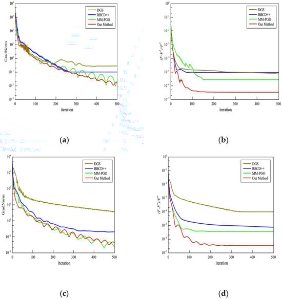
Figure 6.
Optimized performance comparison results of all methods in the Grid(3D) dataset: (a) The Riemannian gradient norm comparison diagram of each method with a 5-node configuration; (b) the relative suboptimality gap comparison diagram of each method with a 5-node configuration; (c) the Riemannian gradient norm comparison diagram of each method with a 10-node configuration; (d) the relative suboptimality gap comparison diagram of each method with a 10-node configuration.
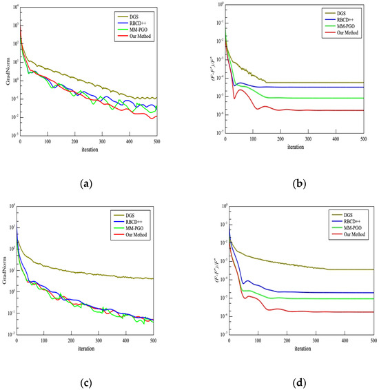
Figure 7.
Optimized performance comparison results of all methods in the Torus(3D) dataset: (a) The Riemannian gradient norm comparison diagram of each method with a 5-node configuration; (b) the relative suboptimality gap comparison diagram of each method with a 5-node configuration; (c) the Riemannian gradient norm comparison diagram of each method with a 10-node configuration; (d) the relative suboptimality gap comparison diagram of each method with a 10-node configuration.
The comparative analysis results of DPGO performance analysis demonstrate that our DPGO algorithm achieves superior performance, exhibiting both higher convergence accuracy and lower computational overhead than other methods.
4.2. Air–Ground Cross-Domain Collaborative SLAM Performance Analysis
Following the evaluation of the DPGO method, we systematically verified the actual performance of our air–ground cross-domain cooperative SLAM method.
We conducted experiments using the GRACO air–ground collaborative dataset [34], which is the first benchmark dataset specifically designed for air–ground cooperative multi-robot SLAM. Developed by Sun Yat-sen University, the dataset includes synchronized data collected from aerial drones and ground vehicles, with both equipped with multi-modal sensors, such as LiDAR, cameras, and GNSS. The GRACO dataset consists of eight aerial sequences and six ground sequences, each providing highly accurate ground truth trajectories. Notably, it contains abundant loop closure features across both aerial and ground sequences. These comprehensive characteristics make GRACO particularly well-suited for evaluating the performance of SLAM algorithms in air–ground cross-domain collaboration and multi-modal fusion scenarios.
We evaluate the method performance on the GRACO dataset using two key metrics, namely absolute trajectory error (ATE) for global accuracy and relative trajectory error (RTE) for local stability [35]. These two metrics jointly evaluate the pose estimation performance of the SLAM system.
To comprehensively evaluate the performance advantages of the proposed method, we compared it with four mainstream SLAM algorithms, namely Lio-Sam [36], Fast-Lio2 [37], ORB-SLAM3 [38], and GAC-Mapping [24]. Table 2 presents the comparative results of pose estimation errors for each method on the sequences of the GRACO dataset. All performance metrics were extracted directly from the original paper.
Table 2.
Results of our method and other methods on the sequences of the GRACO dataset.
The comparison data in Table 2 demonstrate that the proposed method outperforms the other algorithms in pose estimation accuracy across all sequences. In the aerial sequence, Fast-Lio2, GAC-Mapping, and ORB-SLAM3 show significant errors, primarily due to their limited use of altitude information. Although Lio-Sam exhibits a small pose estimation error, the semantics-assisted strategy in our method further enhances pose trajectory estimation accuracy. Our method reduces the mean ATE of each sequence by 0.3494 m, highlighting the effectiveness of the proposed method. In the ground sequence, despite the interference from numerous repeated features, such as railings and trees, the proposed method maintains high pose estimation accuracy through its robust feature-matching mechanism. As a result, its error value remains consistently lower than that of the other methods. The mean ATE of each sequence is reduced by 0.2335 m, 0.5864 m, 5.0058 m, and 0.4981 m, respectively, when compared to Lio-Sam, Fast-Lio2, ORB-SLAM3, and GAC-Mapping. These results demonstrate the exceptional pose estimation accuracy of the proposed method in both ground and aerial sequences, validating its universality and robustness in air–ground cross-domain collaborative SLAM tasks.
To further intuitively evaluate the effectiveness of the proposed method, we conducted a detailed comparative analysis of two representative sequences from the GRACO dataset—the Ground-01 and the Aerial-03 sequences—using three benchmark SLAM methods, namely Lio-Sam, Fast-Lio2, and ORB-SLAM3.
Ground-01 is a loop closure sequence with a relatively high traveling speed, and the absence of distinctive building features poses a significant challenge for feature matching. Figure 8 presents the comparison between the ground truth trajectory and the trajectory estimation by four methods for Ground-01. Specifically, Figure 8a,b display the comparison of the overall trajectory alignment error and the alignment error in each direction for each method on Ground-01, respectively. From the overall trajectory comparison graphs, it is evident that our method achieves the smallest error when compared to the ground truth trajectory. In the latter part of the sequence, as the speed increases, the trajectory and relative rotation errors in the y-direction for the predicted trajectories of other methods increase significantly. However, our method significantly reduces trajectory drift, especially the relative trajectory errors in each direction.
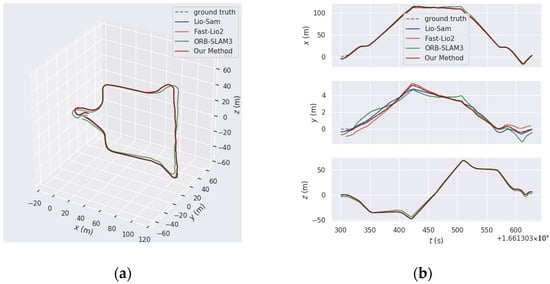
Figure 8.
The comparison results of trajectory estimation by each method and ground truth trajectory on the Ground-01 sequence of the GRACO dataset: (a) The comparison results of trajectory alignment errors of each method; (b) the comparison results of trajectory errors in each direction of each method.
As shown in Figure 9, the comparison results of the ATE evaluation metrics for each method on Ground-01 are presented. From the comparison chart, it is evident that our method outperforms the other methods across all evaluation indicators in this sequence. Specifically, our method reduces the absolute pose estimation error by 0.165, 0.059, and 4.219 compared to Lio-Sam, Fast-Lio2, and ORB-SLAM3, respectively. Among all methods, ORB-SLAM3 performs the worst, with its maximum error reaching 10.089, while our method achieves a significantly lower maximum error of 0.595.
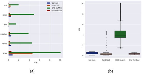
Figure 9.
The ATE comparison results of each method on the Ground-01 sequence of the GRACO dataset: (a) The comparison results of various ATE indicators; (b) the comparison results of the ATE box plots.
As shown in Figure 10, the results of the RTE comparison highlight the superior performance of our method. The evaluation metrics consistently show that the error in our method’s relative pose estimation is lower than that of other comparative methods. Specifically, our method achieves optimal results with a maximum error of 0.099 and a mean error of 0.026. In contrast, ORB-SLAM3 demonstrates the worst performance, with a maximum error of 1.099 during operation. However, the performance differences between Lio-Sam and Fast-Lio2 are not significant. The mean relative pose errors are 0.026 and 0.185, respectively, and the maximum errors are 0.127 and 0.414, respectively. These error values are notably higher than those of our method.
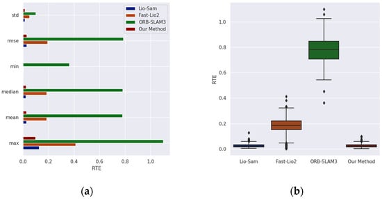
Figure 10.
The RTE comparison results of each method on the Ground-01 sequence of the GRACO dataset: (a) The comparison results of various RTE indicators; (b) the comparison results of the RTE box plots.
The Aerial-03 sequence presents a significant challenge due to the dense, repetitive structures at an altitude of 20 m, which greatly complicate pose estimation. As illustrated in Figure 11, the comparison between the ground truth trajectory and the trajectories generated by each method on the Aerial-03 sequence is shown. Specifically, Figure 11a,b display the overall trajectory alignment error comparison and the trajectory error comparison in each direction for each method on Aerial-03, respectively. Through this comparative analysis, it becomes evident that the error of the method proposed in this paper is considerably lower than that of the other methods. Notably, during mid-flight UAV turning maneuvers, other methods demonstrate significant amplification of z-direction errors, while our proposed method maintains trajectory stability and effectively reduces trajectory drift.
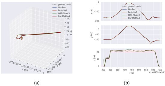
Figure 11.
The comparison results of trajectory estimation by each method and ground truth trajectory in the Aerial-03 sequence of the GRACO dataset: (a) The comparison results of trajectory alignment errors of each method; (b) the comparison results of trajectory errors in each direction of each method.
As shown in Figure 12, the ATE comparison chart for each method on the Aerial-03 sequence is presented. It is evident from the comparison chart that our method outperforms the others in all ATE indicators. The mean absolute error of our method is 0.166, which represents reductions of 0.384, 35.848, and 24.034 compared to Lio-Sam, Fast-Lio2, and ORB-SLAM3, respectively.
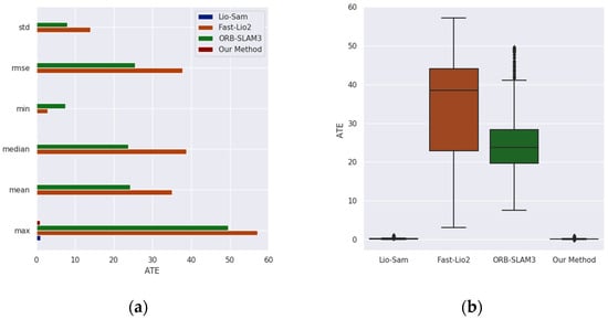
Figure 12.
The ATE comparison results of each method on the Aerial-03 sequence of the GRACO dataset: (a) The comparison results of various ATE indicators; (b) the comparison results of the ATE box plots.
Similarly, Figure 13 presents the RTE comparison chart for each method. The comparison chart clearly illustrates that the relative pose error of our method is significantly lower than that of the other methods. Specifically, our method achieves a mean relative pose error of 0.044 and a maximum error of only 0.272, demonstrating superior stability and accuracy. In comparison, our method reduces the mean relative pose error by 0.175, 16.581, and 4.226 when compared to Lio-Sam, Fast-Lio2, and ORB-SLAM3, respectively.
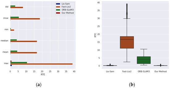
Figure 13.
The RTE comparison results of each method on the Aerial-03 sequence of the GRACO dataset: (a) The comparison results of various RTE indicators; (b) the comparison results of the RTE box plots.
The experimental results validate that the method proposed in this paper exhibits excellent pose estimation performance in both ground sequences and air sequences.
An experimental analysis of the cooperative positioning and mapping performance of our method was then conducted in the UAV and UGV air–ground sequences containing many repetitive loop closures. The experiment evaluated the air–ground collaboration performance of our method by utilizing two groups and three groups of air–ground collaborative UAV and UGV teams, respectively. Table 3 presents the comparative experimental results of air–ground multi-robot cooperative SLAM, using the method proposed in this paper and GAC-Mapping.
Table 3.
Results of our method and other methods on the air–ground collaborative sequences of the GRACO dataset.
The comparative data in Table 3 show that the method proposed in this paper significantly outperforms GAC-Mapping across two air–ground sequence groups. In Team 1, which includes the Aerial-02 sequence and the Ground-04 sequence in GRACO, the mean ATE and RTE were reduced by 1.1885 m and 2.7819 m, respectively. Furthermore, due to the PCM incremental anomaly detection module and multi-level partitioning processing, the total number of parameters was decreased by 18.9%, and the processing delay was shortened by 38.9%. In Team 2, comprising the Aerial-08 sequence, Ground-03 sequence, and Ground-06 sequence in GRACO, the reduction in parameters reached 29.5%. Additionally, the computing delay decreased by 35.6%, and the ATE and RTE were significantly reduced by 0.2387 m and 2.8485 m, respectively. These results indicate that the proposed method achieves an average improvement of 42.7% in trajectory estimation accuracy, along with a 24.2% reduction in resource consumption and a 37.3% increase in operational efficiency. This fully demonstrates the dual advantages of accuracy and efficiency in air–ground cooperative pose estimation.
We verified and analyzed the global trajectory comparison and the details of map construction. To differentiate the mapping areas of each robot, the map information for each robot is independently color-coded. This provides a clear visual representation of the collaboration effect to facilitate the visual assessment of collaborative performance. This enables clear identification of local map construction results of individual robot contributions while maintaining global map consistency.
Figure 14 presents the comparison results between the global trajectory estimation and the ground truth trajectories of our method and GAC-Mapping. The UAV adopts the Aerial-02 sequence in GRACO, while the UGV utilizes the Ground-04 sequence in GRACO. From the comparison results of the global trajectories, it is evident that our method outperforms GAC-Mapping. In particular, the trajectory errors of GAC-Mapping in both the air sequences and the ground sequences are relatively large, while our method’s global trajectory estimation is much closer to the true trajectory. Notably, although individual robot trajectory errors may not always decrease during optimization, the overall system error is significantly reduced. This outcome aligns with expectations: robots with more accurate trajectory estimations help correct mistakes in others, thereby improving the system’s positioning accuracy while maintaining global trajectory consistency. Notably, variations in pose estimation may lead to real-time error increases for certain robots during collaborative optimization, especially during UAV turning maneuvers. However, compared to single-robot SLAM, air–ground cross-domain collaborative SLAM shows clear advantages for large-scale mapping, particularly by improving map completeness and coverage in previously unexplored environments.
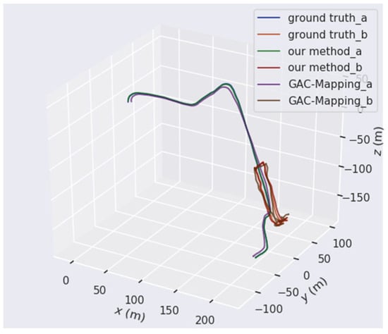
Figure 14.
The comparison results of the ground truth trajectories on the Aerial-02 and the Ground-04 sequences with the cooperative estimated trajectories of our method.
As demonstrated in the map construction effect diagram shown in Figure 15a, our method effectively integrates the local maps of an air–ground robot team composed of a UAV and a UGV into a unified global map. This map is rich in detail, with a high consistency with the actual environment. Additionally, Figure 15b provides a local magnified map detail, clearly illustrating the smooth transition between the road and roadside trees in the scene. The edges of the map are neat, and the low bushes at the environmental corners are accurately identified. These map details comprehensively validate the geometric consistency of the constructed map.
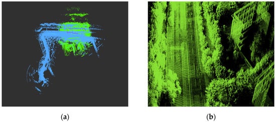
Figure 15.
The air–ground collaborative mapping results of our method on the Aerial-02 and the Ground-04 sequences: (a) The complete map constructed by our method; (b) a partial enlarged view of the map constructed by our method.
Figure 16 compares the trajectory estimation of an air–ground collaborative team, consisting of one UAV and two UGVs, with the ground truth trajectories. The UAV uses the Aerial-08 sequence from the GRACO dataset, while the two UGVs utilize the Ground-03 and Ground-06 sequences, respectively, from the same dataset. The comparison of global trajectories clearly shows that our method outperforms GAC-Mapping. In the intersection area between the air and the ground, GAC-Mapping exhibited significant trajectory errors. In contrast, our method demonstrated the smallest trajectory deviation and lower cumulative error. These results suggest that our method effectively utilizes loop closure detection from both the UAV and UGVs, leading to accurate global trajectory estimation.
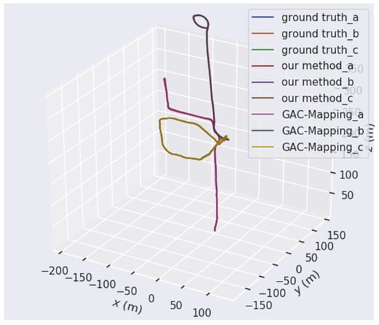
Figure 16.
The comparison results of the ground truth trajectories on the Aerial-08, Ground-03, and Ground-06 sequences with the cooperative estimated trajectories of our method.
The map construction effect, shown in Figure 17a, further highlights our method’s effectiveness in air–ground cross-domain collaborative SLAM tasks. It successfully integrates the map information from both UAVs and UGVs, generating an environment map with rich details and global consistency. Specifically, our method seamlessly merges the local maps of multiple robots into a unified global map. The map not only boasts a high level of detail but also maintains excellent consistency with the actual environment. Additionally, as shown in the magnified local detail map in Figure 17b, the constructed map exhibits high consistency. The transitions between roads, buildings, trees, and other elements along the streets are smooth, the edges are neat, and there are very few outlying points.
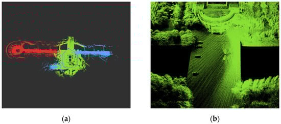
Figure 17.
The air–ground collaborative mapping results of our method on the Aerial-08, Ground-03, and Ground-06 sequences: (a) The complete map constructed by our method; (b) a partial enlarged view of the map constructed by our method.
The comparison results demonstrate our method’s superior performance in air–ground cross-domain collaborative SLAM tasks. In summary, our method significantly enhances both trajectory estimation accuracy and mapping performance for air–ground cross-domain multi-robot SLAM systems. This improvement provides reliable technical support for multi-robot cooperative tasks, especially in complex environments.
5. Discussion
The experimental results on both benchmark SLAM datasets and the air–ground GRACO datasets demonstrate the superior performance of the method proposed in this paper, particularly in large-scale distributed pose graph optimization and air–ground cross-domain SLAM applications. On the benchmark SLAM datasets, the method achieves optimal convergence with minimal iterations in both 5-node and 10-node environments. It excels in complex 10-node scenarios, primarily due to two key techniques, namely loss kernel optimization and multi-level partitioning. The loss kernel optimization technique effectively reduces the error in loop closure detection caused by repeated or complex environments, thus improving the optimization performance in challenging scenarios. Meanwhile, the multi-level partitioning technique divides the global directed pose graph into multiple balanced directed graphs based on the number of robot nodes and their degree of coupling. These graphs are then refined to minimize communication complexity and accelerate convergence. Experiments conducted on the GRACO dataset further validate the proposed method’s exceptional performance in air–ground cross-domain cooperative SLAM, even when there are significant differences in perspectives between UAVs and UGVs. This is achieved through an iterative registration method based on semantic and geometric features assistance, addressing the challenge of large field-of-view differences between UAVs and UGVs. Specifically, this method calculates the high-precision air–ground loop closure transformation matrix by integrating semantic features from the loop closure and performing probabilistic calculations on the geometric features. As a result, global pose estimation accuracy is enhanced. Furthermore, the robustness of the multi-level partitioning majorization–minimization DPGO method incorporating loss kernel optimization contributes to optimal global pose estimation and precise map construction in collaborative scenarios involving multiple UAV and UGV teams. These comprehensive results demonstrate the method’s ability to effectively integrate environmental perception data from both UAVs and UGVs, ensuring consistently high-precision pose estimation and efficient optimization performance in complex and cross-domain collaborative tasks.
Although the method demonstrates excellent performance and robustness, some limitations remain. First, it has only been validated with public datasets, and its performance has not yet been tested in real-world, complex environments. As a result, verifying its performance in the face of real-world challenges, such as sensor noise, is difficult. Additionally, as the method’s performance improves, the communication complexity between robot nodes increases, which may negatively impact operational efficiency and performance, particularly in environments with limited computational resources or memory. However, comparison results of the running parameters and consumption time with other methods show that this method, through techniques, such as PCM incremental anomaly discrimination, multi-level partitioning, and loss kernel optimization, achieves strong generalization across diverse scenarios. It outperforms existing methods in both resource consumption during operation and robustness.
6. Conclusions
This paper proposes a distributed multi-robot collaborative SLAM method based on air–ground cross-domain cooperation, achieving high-precision collaborative SLAM by fusing environmental features from both UAVs and UGVs. The method begins with a local single-robot SA-LIO at each robot’s front end, which extracts local keyframes of the surrounding environment in real time. When UAVs and UGVs enter the communication range, they exchange loop closure keyframes and utilize a PCM incremental anomaly detection method to eliminate incorrect loop closures, ensuring reliable data association. Next, an iterative registration method based on semantic and geometric features assistance computes the relative coordinate transformation matrix between heterogeneous keyframes. This step establishes a unified coordinate system and provides accurate initial pose estimates for backend optimization. Finally, a multi-level partitioning majorization–minimization DPGO method incorporating loss kernel optimization ensures smooth convergence of the optimization process to first-order critical points, enabling precise global localization and mapping for both air–ground UAV and UGV teams. Experimental results on benchmark SLAM datasets and the GRACO dataset demonstrate that our method achieves state-of-the-art performance in air–ground cross-domain collaborative SLAM compared to other approaches.
In the future, we will continue to explore more accurate and reliable algorithm improvements, utilizing advanced techniques, such as chordal initialization and spectral relaxation, to reduce communication complexity and enhance optimization efficiency. Additionally, we plan to extend the proposed method from public datasets to real-world environments, ensuring optimal system performance. These advancements will significantly contribute to the deployment of air–ground cross-domain multi-robot systems in practical application scenarios.
Author Contributions
Conceptualization, Y.B.; Data curation, X.J.; Methodology, Y.B.; Software, Y.B.; Supervision, P.L. and C.W.; Validation, P.L.; Writing—original draft, Y.B.; Writing—review and editing, Y.B., P.L., C.W. and X.J. All authors have read and agreed to the published version of the manuscript.
Funding
This research was funded by Jilin Province Science and Technology Development Plan Project, grant number 20250102228JC.
Data Availability Statement
The original contributions presented in this study are included in the article. Further inquiries can be directed to the corresponding author.
Conflicts of Interest
The authors declare no conflicts of interest.
Abbreviations
The following abbreviations are used in this manuscript:
| CSLAM | Collaborative simultaneous localization and mapping |
| UAV | Unmanned aerial vehicle |
| UGV | Unmanned ground vehicle |
| PCM | Pairwise consistency maximization |
| DPGO | Distributed pose graph optimization |
References
- Jiang, W.; Xue, H.; Si, S.; Xiao, L.; Zhao, D.; Zhu, Q.; Nie, Y.; Dai, B. R2SCAT-LPR: Rotation-Robust Network with Self- and Cross-Attention Transformers for LiDAR-Based Place Recognition. Remote Sens. 2025, 17, 1057. [Google Scholar] [CrossRef]
- Barbieri, L.; Tedeschini, B.C.; Brambilla, M.; Nicoli, M. Deep Learning-Based Cooperative LiDAR Sensing for Improved Vehicle Positioning. IEEE Trans. Signal Process. 2024, 72, 1666–1682. [Google Scholar] [CrossRef]
- Chang, Y.; Hughes, N.; Ray, A.; Carlone, L. Hydra-Multi: Collaborative Online Construction of 3D Scene Graphs with Multi-Robot Teams. In Proceedings of the 2023 IEEE/RSJ International Conference on Intelligent Robots and Systems (IROS), Detroit, MI, USA, 1–5 October 2023; pp. 10995–11002. [Google Scholar]
- Xu, H.; Liu, P.; Chen, X.; Shen, S. D2SLAM: Decentralized and Distributed Collaborative Visual-Inertial SLAM System for Aerial Swarm. IEEE Trans. Robot. 2024, 40, 3445–3464. [Google Scholar] [CrossRef]
- Araújo, A.G.; Pizzino, C.A.P.; Couceiro, M.S.; Rocha, R.P. A Multi-Drone System Proof of Concept for Forestry Applications. Drones 2025, 9, 80. [Google Scholar] [CrossRef]
- Chen, Z.; Zhao, J.; Feng, T.; Ye, C.; Xiong, L. Robust Loop Closure Selection Based on Inter-Robot and Intra-Robot Consistency for Multi-Robot Map Fusion. Remote Sens. 2023, 15, 2796. [Google Scholar] [CrossRef]
- Xie, Y.; Zhang, Y.; Chen, L.; Cheng, H.; Tu, W.; Cao, D. RDC-SLAM: A Real-Time Distributed Cooperative SLAM System Based on 3D LiDAR. IEEE Trans. Intell. Transp. Syst. 2022, 23, 14721–14730. [Google Scholar] [CrossRef]
- Li, Z.; Xu, P.; Ding, L.; Shan, J.; Yang, W.; Deng, Z.; Gao, H.; Liu, T.; Yang, H. Enhancing Cooperative Exploration and Planning: UAV-Legged Robot Synergy. IEEE Robot. Autom. Lett. 2024, 9, 10367–10374. [Google Scholar] [CrossRef]
- Miller, I.D.; Cladera, F.; Smith, T.; Taylor, C.J.; Kumar, V. Stronger Together: Air-Ground Robotic Collaboration Using Semantics. IEEE Robot. Autom. Lett. 2022, 7, 9643–9650. [Google Scholar] [CrossRef]
- Munguia, R.; Grau, A.; Bolea, Y.; Obregón-Pulido, G. A Simultaneous Control, Localization, and Mapping System for UAVs in GPS-Denied Environments. Drones 2025, 9, 69. [Google Scholar] [CrossRef]
- Rosen, D.M.; Carlone, L.; Bandeira, A.S.; Leonard, J.J. SE-Sync: A certifiably correct algorithm for synchronization over the special Euclidean group. Int. J. Robot. Res. 2019, 38, 95–125. [Google Scholar] [CrossRef]
- Yu, Z.; Qiao, Z.; Qiu, L.; Yin, H.; Shen, S. Multi-Session, Localization-Oriented and Lightweight LiDAR Mapping Using Semantic Lines and Planes. In Proceedings of the 2023 IEEE/RSJ International Conference on Intelligent Robots and Systems (IROS), Detroit, MI, USA, 1–5 October 2023; pp. 7210–7217. [Google Scholar]
- Huang, Y.; Shan, T.; Chen, F.; Englot, B. DiSCo-SLAM: Distributed Scan Context-Enabled Multi-Robot LiDAR SLAM With Two-Stage Global-Local Graph Optimization. IEEE Robot. Autom. Lett. 2022, 7, 1150–1157. [Google Scholar] [CrossRef]
- Lajoie, P.; Beltrame, G. Swarm-SLAM: Sparse Decentralized Collaborative Simultaneous Localization and Mapping Framework for Multi-Robot Systems. IEEE Robot. Autom. Lett. 2024, 9, 475–482. [Google Scholar] [CrossRef]
- Zhong, S.; Qi, Y.; Chen, Z.; Wu, J.; Chen, H.; Liu, M. DCL-SLAM: A Distributed Collaborative LiDAR SLAM Framework for a Robotic Swarm. IEEE Sens. J. 2024, 24, 4786–4797. [Google Scholar] [CrossRef]
- Mangelson, J.G.; Dominic, D.; Eustice, R.M.; Vasudevan, R. Pairwise Consistent Measurement Set Maximization for Robust Multi-Robot Map Merging. In Proceedings of the 2018 IEEE International Conference on Robotics and Automation (ICRA), Brisbane, QLD, Australia, 21–25 May 2018; pp. 2916–2923. [Google Scholar]
- Choudhary, S.; Carlone, L.; Nieto, C.; Rogers, J.; Christensen, H.; Dellaert, F. Distributed trajectory estimation with privacy and communication constraints: A two-stage distributed Gauss-Seidel approach. In Proceedings of the 2016 IEEE International Conference on Robotics and Automation (ICRA), Stockholm, Sweden, 16–21 May 2016; pp. 5261–5268. [Google Scholar]
- Tian, Y.; Koppel, A.; Bedi, A.S.; How, J.P. Asynchronous and Parallel Distributed Pose Graph Optimization. IEEE Robot. Autom. Lett. 2020, 5, 5819–5826. [Google Scholar] [CrossRef]
- Tian, Y.; Chang, Y.; Arias, F.H.; Nieto-Granda, C.; How, J.P.; Carlone, L. Kimera-Multi: Robust, Distributed, Dense Metric-Semantic SLAM for Multi-Robot Systems. IEEE Trans. Robot. 2022, 38, 2022–2038. [Google Scholar] [CrossRef]
- Yang, H.; Antonante, P.; Tzoumas, V.; Carlone, L. Graduated Non-Convexity for Robust Spatial Perception: From Non-Minimal Solvers to Global Outlier Rejection. IEEE Robot. Autom. Lett. 2020, 5, 1127–1134. [Google Scholar] [CrossRef]
- Fan, T.; Murphey, T. Majorization Minimization Methods for Distributed Pose Graph Optimization. IEEE Trans. Robot. 2024, 40, 22–42. [Google Scholar] [CrossRef]
- Nesterov, Y. Introductory Lectures on Convex Optimization: A Basic Course; Springer Science & Business Media: Berlin, Germany, 2013. [Google Scholar]
- Li, C.; Guo, G.; Yi, P.; Hong, Y. Distributed Pose-Graph Optimization with Multi-Level Partitioning for Multi-Robot SLAM. IEEE Robot. Autom. Lett. 2024, 9, 4926–4933. [Google Scholar] [CrossRef]
- He, J.; Zhou, Y.; Huang, L.; Kong, Y.; Cheng, H. Ground and Aerial Collaborative Mapping in Urban Environments. IEEE Robot. Autom. Lett. 2021, 6, 95–102. [Google Scholar] [CrossRef]
- Liu, D.; Wu, J.; Du, Y.; Zhang, R.; Cong, M. SBC-SLAM: Semantic Bioinspired Collaborative SLAM for Large-Scale Environment Perception of Heterogeneous Systems. IEEE Trans. Instrum. Meas. 2024, 73, 5018110. [Google Scholar] [CrossRef]
- Duan, X.; Wu, M.; Xiong, C.; Hu, Q.; Zhao, P. A Base-Map-Guided Global Localization Solution for Heterogeneous Robots Using a Co-View Context Descriptor. Remote Sens. 2024, 16, 4027. [Google Scholar] [CrossRef]
- Qiao, X.; Tang, J.; Li, G.; Yang, W.; Shen, B.; Niu, W.; Xie, W.; Peng, X. SMR-GA: Semantic Map Registration Under Large Perspective Differences Through Genetic Algorithm. IEEE Robot. Autom. Lett. 2025, 10, 2518–2525. [Google Scholar] [CrossRef]
- Liu, P.; Bi, Y.; Shi, J.; Zhang, T.; Wang, C. Semantic-Assisted LIDAR Tightly Coupled SLAM for Dynamic Environments. IEEE Access 2024, 12, 34042–34053. [Google Scholar] [CrossRef]
- Zhong, Y. Intrinsic shape signatures: A shape descriptor for 3D object recognition. In Proceedings of the 2009 IEEE 12th International Conference on Computer Vision Workshops, Kyoto, Japan, 27 September–4 October 2009; pp. 689–696. [Google Scholar]
- Tian, Y.; Khosoussi, K.; Rosen, D.M.; How, J.P. Distributed Certifiably Correct Pose-Graph Optimization. IEEE Trans. Robot. 2021, 37, 2137–2156. [Google Scholar] [CrossRef] [PubMed]
- Fan, T.; Murphey, T. Majorization Minimization Methods for Distributed Pose Graph Optimization with Convergence Guarantees. In Proceedings of the 2020 IEEE/RSJ International Conference on Intelligent Robots and Systems (IROS), Las Vegas, NV, USA, 24 October 2020; pp. 5058–5065. [Google Scholar]
- Barron, J.T. A General and Adaptive Robust Loss Function. In Proceedings of the 2019 IEEE/CVF Conference on Computer Vision and Pattern Recognition (CVPR), Long Beach, CA, USA, 15–20 June 2019; pp. 4326–4334. [Google Scholar]
- Xu, H.; Shen, S. BDPGO: Balanced Distributed Pose Graph Optimization Framework for Swarm Robotics. arXiv 2021, arXiv:2109.04502. [Google Scholar]
- Zhu, Y.; Kong, Y.; Jie, Y.; Xu, S.; Cheng, H. GRACO: A Multimodal Dataset for Ground and Aerial Cooperative Localization and Mapping. IEEE Robot. Autom. Lett. 2023, 8, 966–973. [Google Scholar] [CrossRef]
- Evo: Python PackAge for the Evaluation of Odometry and SLAM. Available online: https://github.com/MichaelGrupp/evo (accessed on 19 November 2017).
- Shan, T.; Englot, B.; Meyers, D.; Wang, W.; Ratti, C.; Rus, D. LIO-SAM: Tightly-coupled Lidar Inertial Odometry via Smoothing and Mapping. In Proceedings of the 2020 IEEE/RSJ International Conference on Intelligent Robots and Systems (IROS), Las Vegas, NV, USA, 25–29 October 2020; pp. 5135–5142. [Google Scholar]
- Xu, W.; Cai, Y.; He, D.; Lin, J.; Zhang, F. FAST-LIO2: Fast Direct LiDAR-Inertial Odometry. IEEE Trans. Robot. 2022, 38, 2053–2073. [Google Scholar] [CrossRef]
- Campos, C.; Elvira, R.; Rodríguez, J.J.G.; Montiel, J.M.M.; Tardós, J.D. ORB-SLAM3: An Accurate Open-Source Library for Visual, Visual–Inertial, and Multimap SLAM. IEEE Trans. Robot. 2021, 37, 1874–1890. [Google Scholar] [CrossRef]
Disclaimer/Publisher’s Note: The statements, opinions and data contained in all publications are solely those of the individual author(s) and contributor(s) and not of MDPI and/or the editor(s). MDPI and/or the editor(s) disclaim responsibility for any injury to people or property resulting from any ideas, methods, instructions or products referred to in the content. |
© 2025 by the authors. Licensee MDPI, Basel, Switzerland. This article is an open access article distributed under the terms and conditions of the Creative Commons Attribution (CC BY) license (https://creativecommons.org/licenses/by/4.0/).