Adaptability Study of an Unmanned Aerial Vehicle Actuator Fault Detection Model for Different Task Scenarios

Abstract

Unmanned aerial vehicles (UAVs) may encounter actuator faults in diverse flight scenarios, requiring robust fault detection models that can adapt to varying data distributions. To address this challenge, this paper proposes an approach that integrates Domain-Adversarial Neural Networks (DANNs) with a Mixture of Experts (MoE) framework. By employing domain-adversarial learning, the method extracts domain-invariant features, mitigating distribution discrepancies between source and target domains. The MoE architecture dynamically selects specialized expert models based on task-specific data characteristics, improving adaptability to multimodal environments. This integration enhances fault detection accuracy and robustness while maintaining efficiency under constrained computational resources. To validate the proposed model, we conducted flight experiments, demonstrating its superior performance in actuator fault detection compared to conventional deep learning methods. The results highlight the potential of MoE-enhanced domain adaptation for real-time UAV fault detection in dynamic and uncertain environments.

1. Introduction

Unmanned aerial vehicles (UAVs), particularly fixed-wing models, are widely utilized in surveillance, mapping, and other applications due to their intelligence, efficiency, and long-range capabilities [1,2,3,4]. Actuator faults in control surfaces, such as ailerons, elevators, and rudders, can cause abnormal fluctuations in flight parameters, compromising stability and risking system failures. Efficient and accurate fault detection is thus critical to enhancing UAV reliability and safety in dynamic environments.

Recent advances in fault detection have significantly shaped the field, particularly through data-driven and transfer learning approaches. Data-driven methods leverage historical and real-time data to model system-fault correlations, offering high accuracy. For instance, multi-sensor systems integrating visual, acoustic, and thermal data enable anomaly detection in dynamic settings [5,6], while extreme learning machines (ELMs) provide rapid structural damage identification via vibration analysis [7,8]. In UAV applications, semi-supervised support vector machines (SVMs) and hybrid deep neural networks (HDNNs) with multi-time-window CNN-BiLSTM improve anomaly and hazard identification [9,10]. However, the aforementioned data-driven fault detection methods typically rely on a large amount of labeled data and assume that the training and testing data distributions are consistent [11,12]. The diversity of UAV mission environments and operational conditions leads to significant differences between the training and testing data distributions. These distribution shifts pose major challenges for UAV fault detection in dynamic environments [13]. Traditional data-driven methods often lack the ability to transfer and generalize effectively when facing new environments and tasks, limiting their capacity to accurately identify potential faults and reducing the reliability of the detection system [14].

To address distribution shifts, transfer learning—particularly domain adaptation—extracts domain-invariant features to enable cross-domain knowledge transfer [15,16]. Notable methods include Res-BPNN with multi-layer MK-MMD for aeroengine monitoring [17], federated neural networks for sensor fault detection [18], and 1D convolutional networks enhanced with adaptive batch normalization and Grey Wolf Optimization for multirotor UAV diagnostics [19]. Liu et al. [20] employed ensemble transfer learning to aggregate multi-UAV data, mitigating single-source data limitations, but its static ensemble approach lacks dynamic adaptability to diverse flight conditions. Additionally, Maximum Mean Discrepancy (MMD)-based methods struggle to align complex, nonlinear distributions. While effective, these approaches often rely on computationally intensive models or struggle with multimodal data heterogeneity.

To overcome these adaptability challenges, Domain-Adversarial Neural Networks (DANNs) provide a robust domain adaptation solution by learning domain-invariant features through adversarial training [21]. In UAV actuator fault detection, a DANN’s primary advantages include aligning feature distributions between labeled source domains and unlabeled target domains, significantly reducing reliance on extensive labeled fault data—a critical benefit, given their scarcity in UAV applications. By pitting a domain classifier against a task classifier, a DANN forces the feature extractor to produce domain-indistinguishable features, mitigating environmental variations like wind-induced distribution shifts. This has proven effective in noisy conditions, such as gear and bearing diagnostics [22,23], making a DANN suitable for UAV cross-domain challenges. The motivation for selecting a DANN lies in its computational efficiency compared to multi-layer MMD, integrating adversarial training within a single neural network to minimize overhead. Moreover, a DANN’s ability to generalize without target domain labels aligns with UAV real-time fault detection needs in untested environments.

Despite these advances, UAV actuator fault detection remains underexplored, particularly in addressing multimodal data distributions, fault–effect confusion, and computational constraints. First, varying environmental conditions cause significant distribution shifts, which existing methods inadequately address. Second, the contradiction between instantaneous fault onset (e.g., stuck faults causing gradual heading changes) and sustained effects (e.g., loose faults inducing oscillations) complicates feature extraction, often leading to confusion with normal fluctuations. Third, achieving high cross-domain accuracy under limited computational resources is rarely prioritized, reducing reliability in real-time UAV applications. These challenges necessitate a fault detection approach that simultaneously handles multimodal data heterogeneity, distinguishes fault effects from environmental variations, and meets the computational constraints of onboard systems.

To address these gaps and overcome the limitations of the DANN’s simple classifiers, which struggle to distinguish multimodal data patterns, this study proposes a fault detection method integrating the DANN with a Mixture of Experts (MoE) framework. This approach leverages the DANN’s ability to extract domain-invariant features to mitigate distribution shifts, while the MoE’s gating mechanism dynamically selects specialized expert networks to enhance adaptability to multimodal data distributions and resolve fault–effect confusion [24]. Unlike Liu et al.’s static ensemble approach [20], which lacks flexibility in variable flight scenarios, the MoE’s dynamic expert selection significantly improves fault detection performance, particularly in distinguishing instantaneous and sustained fault effects. Furthermore, the MoE’s sparse activation reduces computational load, ensuring efficiency in resource-constrained UAV systems. Flight experiments validate the method’s superior fault detection rate (FDR) and false alarm rate (FAR), demonstrating its robustness and practical value.

The main contributions of this paper are as follows:

(1) This paper proposes a method combining the MoE model and a DANN for UAV actuator fault detection. By employing domain-adversarial learning, the method extracts domain-invariant features to address data distribution discrepancies. Additionally, it integrates a gating mechanism to dynamically select the optimal expert network, thereby improving detection accuracy and robustness while overcoming the limitations of single classifiers in handling multimodal data.

(2) The effectiveness of the proposed method is validated through flight experiments using real flight data. The results demonstrate that the method achieves precise actuator fault detection in multi-task environments, showcasing strong practical value and reliability.

The remainder of this paper is organized as follows: Section 2 discusses the impact of environmental factors on UAV actuator fault detection. Section 3 introduces the proposed domain adaptation method enhanced by the MoE model. Section 4 presents experimental results to verify the effectiveness of the method. Finally, Section 5 concludes the paper.

2. Problem Description

2.1. Description of Different Task Scenarios

This study focuses on fixed-wing unmanned aerial vehicles (FW-UAVs), which rely on control surfaces such as ailerons, elevators, and rudders, making them particularly susceptible to actuator faults under varying environmental conditions.

Wind direction and wind speed are significant environmental factors that influence UAV flight dynamics—especially under actuator fault conditions, where their interference becomes more pronounced. In low-wind conditions, actuator faults may cause noticeable changes in trajectory. However, in moderate to strong winds, their effects can be masked by natural flight fluctuations caused by turbulence, increasing the likelihood of false alarms or missed detections. This poses a challenge for fault detection models, as sensor data collected under such conditions can exhibit patterns similar to those induced by actuator faults.

To formally describe these environmental influences, wind speed and direction are represented as a two-dimensional vector: $w={[v,\theta ]}^T$. The UAV motion is governed by a nonlinear six-degree-of-freedom (6-DOF) model based on the Newton–Euler equations:

$$\dot{x}(t)=f(x(t),u(t),w(t)),$$

(1)

where $x(t)$ is the UAV’s state vector (e.g., position, velocity, pitch, roll, yaw), $u(t)$ is the control input (e.g., thrust, aileron, rudder), and $w(t)$ represents wind-related environmental inputs. This equation models how actuator faults alter $u(t)$, affecting $x(t)$, which is key for fault detection in Section 2.2.

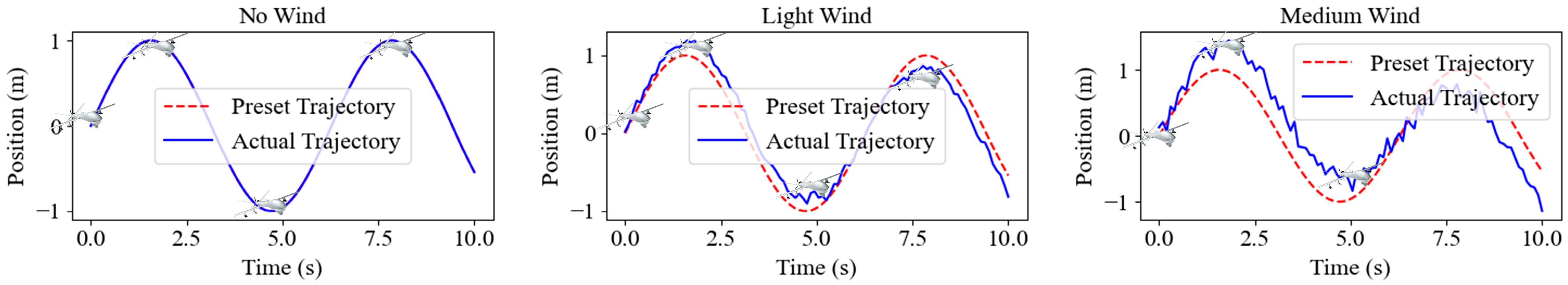
Figure 1 illustrates the simulated flight trajectories under different wind speeds: the trajectory remains stable in no wind conditions, slightly deviates under light winds, and significantly deviates under middle winds, requiring dynamic adjustments. Trajectories are plotted in a 2D coordinate system (x, y) with the UAV’s starting position at (0, 0), where negative y-values indicate positions south of the origin, and positive y-values indicate positions north of the origin.

These trajectories were obtained through numerical simulations using a nonlinear six-degree-of-freedom (6-DOF) UAV dynamic model based on Newton–Euler equations. The UAV was commanded to maintain a constant heading and altitude throughout the simulation, with no actuator faults injected. To isolate the impact of wind, all control parameters and initial conditions were held constant across different scenarios. Wind was introduced as a steady external disturbance vector. Three wind conditions were simulated: no wind (0 m/s), light wind (2 m/s), and middle wind (5 m/s), with a fixed direction. Each trajectory corresponds to the UAV’s response under a specific wind condition over a fixed simulation time. These results highlight the challenge for fault detection models in distinguishing between normal wind-induced deviations and those caused by actuator faults, which is critical to reducing false alarms and missed detections.

The changes in wind speed and direction are reflected in the input features of the fault detection model through sensor data. There exists a nonlinear mapping relationship between the sensor data and the flight state and environmental factors $w(t)$:

$$z(t)=g(x(t),w(t)),$$

(2)

where, $z(t)$ represents the extracted feature vector obtained by mapping the raw sensor measurements $x(t)$ and environment factors $w(t)$ into a compact feature space using the neural network-based feature extractor $g(\cdot )$.

2.2. Characteristics of Actuator Fault in UAVs

Actuator faults are a critical issue in UAV systems, directly affecting the control input $u(t)$, which in turn alters the state vector $x(t)$. This study focuses on two typical actuator faults in control surfaces: stuck faults and loose faults.

(1) Stuck fault: The actuator becomes fixed at a specific position, rendering the control surface immovable. For instance, a rudder may lock at a certain deflection angle, causing $u(t)$ to exhibit a constant deviation, leading to sustained changes in $x(t)$, such as an unintended yaw rate or trajectory drift.

(2) Loose fault: Due to a failure in the hinge torque, the control surface oscillates freely under aerodynamic forces. In this case, $u(t)$ shows erratic fluctuations, resulting in high-frequency disturbances in $x(t)$, such as rapid oscillations in pitch or roll angles.

These faults occur abruptly, representing sudden actuator failures. However, due to the UAV’s aerodynamic characteristics (e.g., inertia, damping, and aerodynamic forces), the impact on $x(t)$ is sustained rather than transient. For example, a stuck fault may gradually alter the heading, while a loose fault induces continuous oscillations that blend with normal flight variations.

Fault detection requires extracting features from sensor data. The input to the fault detection model is the extracted feature set $x(t)$, which includes features extracted from sensor data. These features are closely related to environmental factors. The features of the model input $x_f$ are obtained by mapping the sensor data and environmental factors:

$$x_f=\phi (z(t),w(t)),$$

(3)

where $\phi (\cdot )$ is the feature extraction function, which maps the sensor data and environmental factors to the feature space.

However, feature extraction faces the following difficulties:

(1) Fault–effect confusion: The aerodynamic smoothing makes it challenging to distinguish fault-induced changes in $x(t)$ from normal fluctuations. For example, the heading deviation from a stuck fault may resemble a wind effect, while the oscillations from a loose fault may be mistaken for turbulence.

(2) Contradiction between instantaneous onset and sustained effects: The abrupt onset of faults leads to sustained effects, requiring the model to capture both the initial anomaly and its prolonged impact, increasing the complexity of feature extraction.

These characteristics necessitate a fault detection method capable of accurately identifying subtle and sustained fault patterns.

2.3. Challenges of Fault Detection Models in Different Task Scenarios

Changes in wind speed and wind direction can lead to data distribution shifts, which is a core challenge faced by many traditional fault detection models.

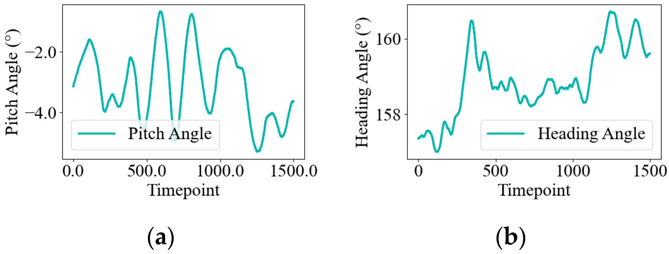
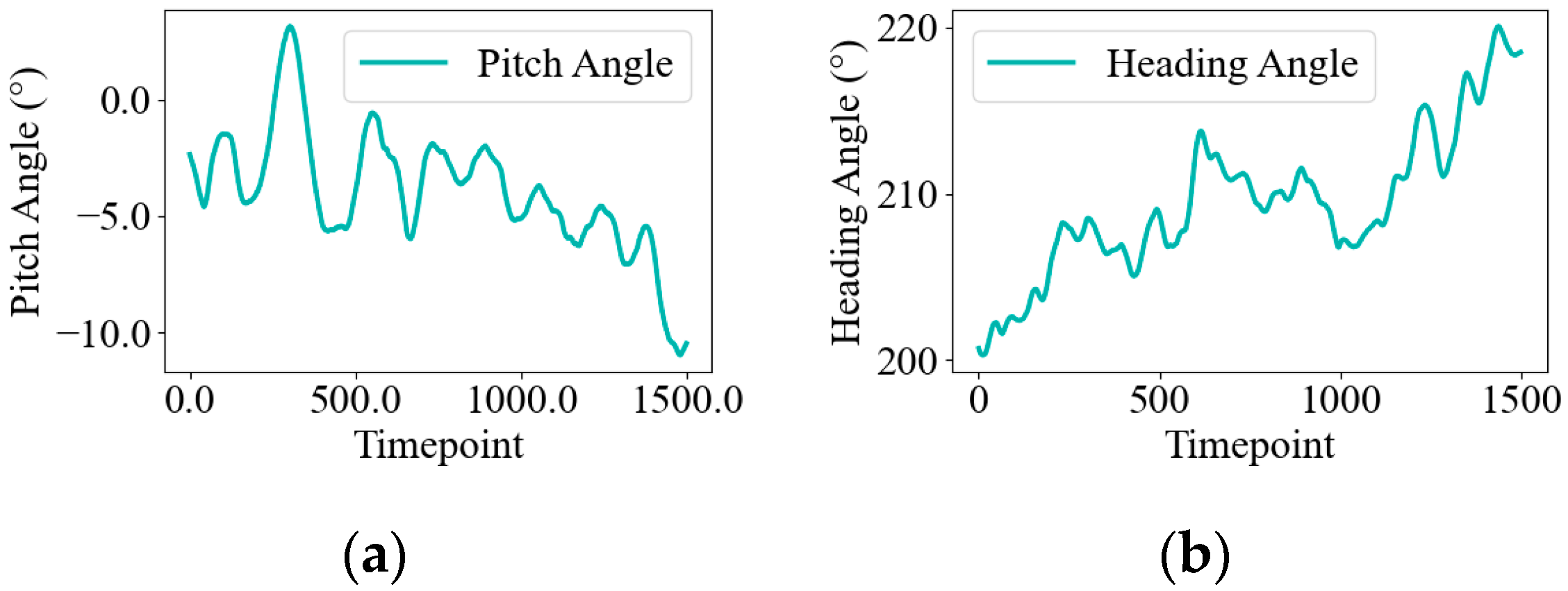
(1) The training data are collected in a specific environment, while testing scenarios often differ, leading to significant distribution shifts. Figure 2 and Figure 3 illustrate such shifts in pitch and heading angles during normal flights under varying wind conditions. Figure 2 (11 September 2024, no wind) shows stable posture and navigation with small, low-frequency fluctuations. In contrast, Figure 3 (1 September 2024, strong wind) presents irregular, high-amplitude oscillations, indicating wind-induced instability. These differences highlight the challenge of ensuring robust generalization in fault detection models across changing conditions. Specifically, such distribution shifts can cause the model to misinterpret wind-induced variations as faults, increasing the risk of false positives or missed detections. This underscores the need for advanced fault detection methods that can adapt to diverse environmental conditions while maintaining high accuracy and reliability.

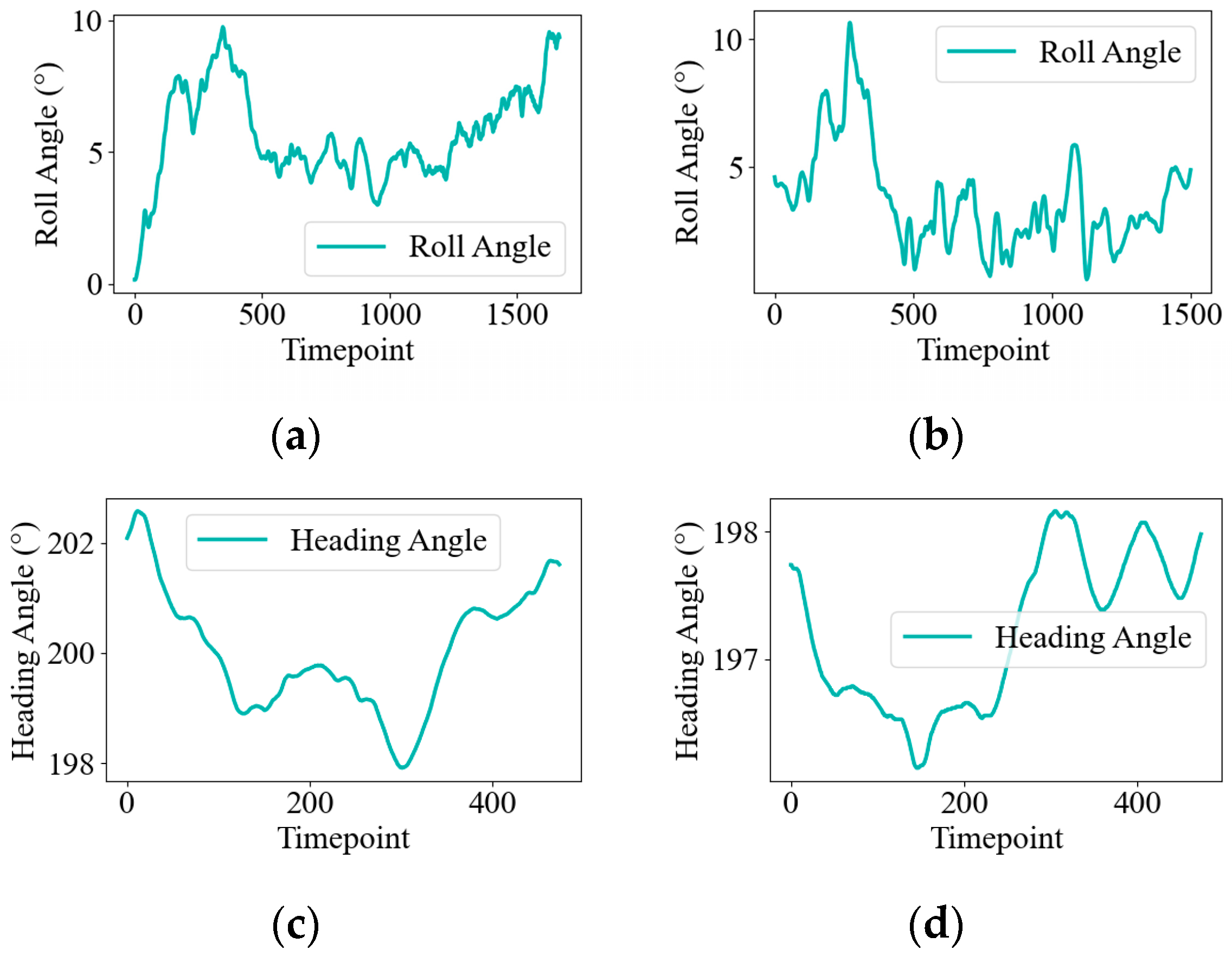
(2) Performance degradation of a single classifier model: In strong wind conditions, fluctuations in flight attitude data are often misjudged as faults, degrading model performance. As shown in Figure 4, normal roll and heading angles under strong wind exhibit high-frequency, irregular fluctuations due to wind interference, resembling the oscillations caused by loose faults under no-wind conditions. Specifically, subfigures (a) and (b) compare roll angles in strong wind (normal) and no wind (loose fault), both showing rapid, high-frequency oscillations with similar amplitudes. Similarly, subfigures (c) and (d) reveal that heading angle variations under strong wind mimic the erratic fluctuation patterns of loose faults, particularly in their frequency and irregularity. These similarities make it difficult to distinguish normal variations from actual faults, leading to higher misclassification rates and underscoring the limitations of single-classifier models in complex, variable environments.

3. UAV Actuator Fault Detection Based on Improved Domain Adaptation

To address the issues of data distribution inconsistency and misjudgment in UAV actuator fault detection, this paper proposes a method that integrates domain adaptation with an MoE framework. By extracting domain-invariant features and dynamically adapting to multimodal data, this approach enhances both the accuracy and robustness of fault detection across diverse task scenarios.

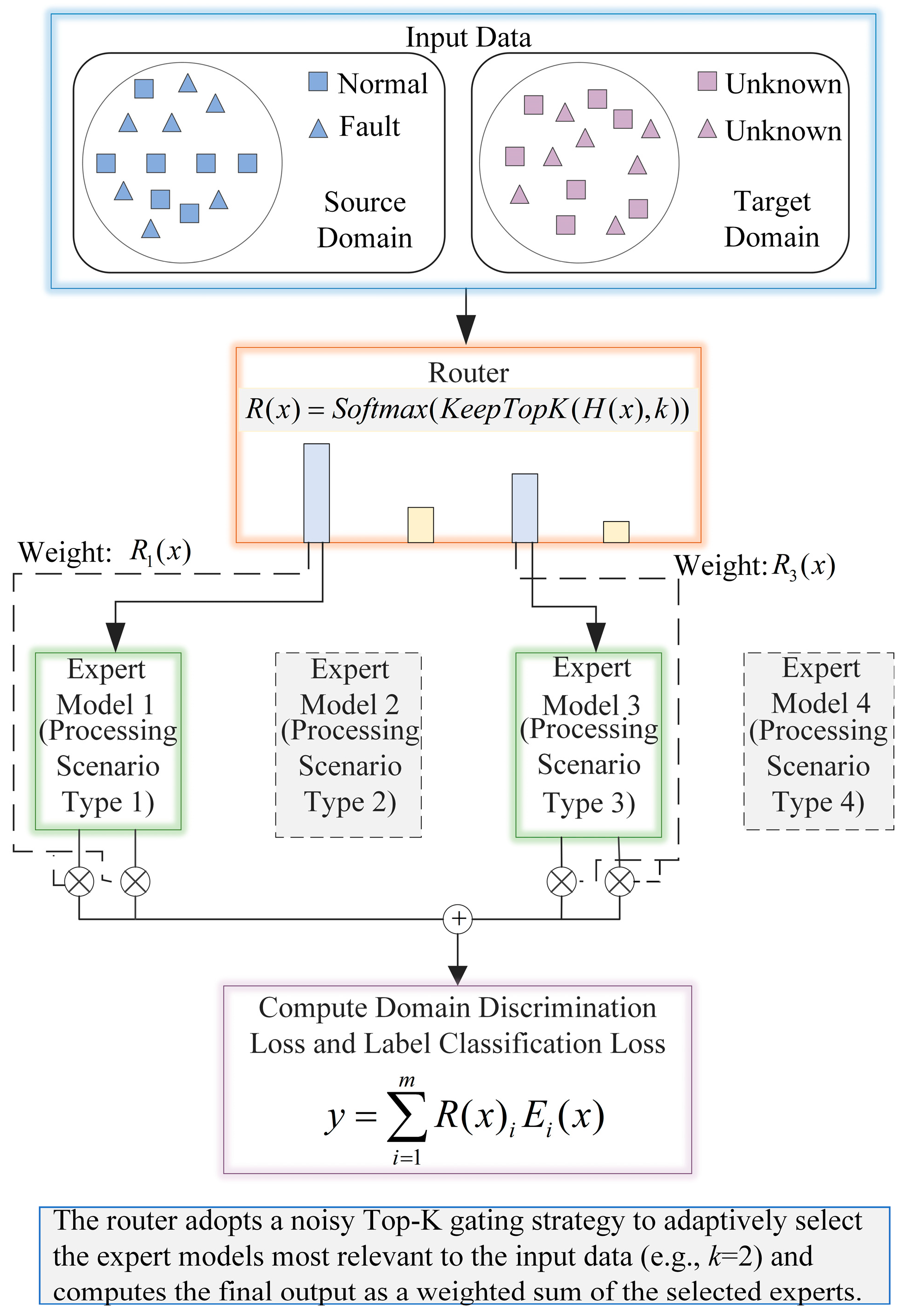
As illustrated in Figure 5, the proposed framework begins by feeding the UAV sensor data into a shared feature extractor. The extracted features are then passed to a gating network, which assigns soft weights to determine how the input is routed to multiple expert models. Each expert is implemented as a DANN, allowing it to learn features that are both task-relevant and invariant across different domains. The outputs of these experts are finally aggregated based on the weights assigned by the gating network, enabling the model to make adaptive and reliable fault detection decisions.

The method leverages a DANN within the MoE framework to align feature distributions between source and target domains while employing a gating mechanism to dynamically select optimal expert networks for specific data modalities. The following subsections elaborate on the formal problem description, the MoE architecture, and its training process.

3.1. The Formal Description of the Domain Adaptation Problem

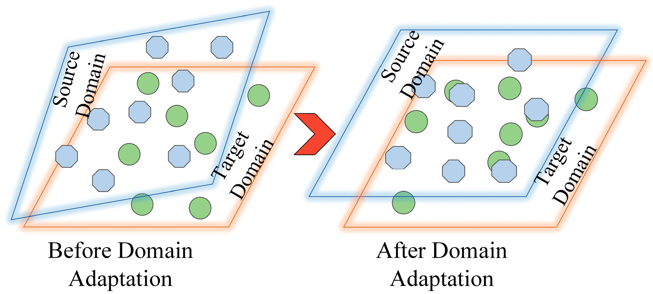
In UAV multi-task scenarios, due to environmental factors such as wind speed and wind direction, there is often a significant distribution shift between the training set (source domain) and the test set (target domain), which leads to a performance drop of traditional fault detection models in the target domain. To address this, this paper introduces domain adaptation methods, aiming to optimize the model to reduce the distribution shift between the source and target domains. By aligning the feature distributions across domains, the model becomes better suited for generalization to the target domain. Figure 6 visually represents this domain adaptation process. The following sections will describe the domain adaptation problem from a formal perspective.

Define the input set as $X$ and the binary labels as $Y=\{0,1\}$. On $X$, a domain is defined as a pair $<D,f>$, where $D$ is a distribution function that describes the probability of each sample in $X$, and $f$ is a labeling function $f:X\to [0,1]$.

Given $M$ source domains, the joint distribution of the data is represented as Equation (4). Specifically, $D(x)$ denotes the probability of input samples $x\in X$, and $f(x):X\to \{0,1\}$ is the true labeling function assigning binary fault labels (0 for normal, 1 for fault) to $x$. $P(x,y)$ is the joint probability distribution of input $x$ and label $y$, consistent with the Bayesian formulation.

Considering $P_{S^i}(x,y)\ne P_{S^j}(x,y),1\le i\ne j\le M$, it indicates that the data distributions differ between domains. The differences in data distribution are caused by $D_{S^i}\ne D_{S^j}$ while $f(x)$ remains unchanged across domains.

$$P(x,y)=P(x)P(y|x)=D(x)f(x)$$

(4)

For a new scenario defined as the target domain $<D_T,f>$, it is necessary to design an algorithm to learn a classifier $h:X\to Y,h\in H$ (where $H$ is a hypothetical space) that approximates $f$. Define the discrepancy between $h$ and $f$ in the target domain as the risk: $\epsilon (h,f;D_T)={\mathbb{E}}_{x~D_T}\left|h(x)-f(x)\right|$; then the goal is to find $\min h\in H\in (h,f;D_T)$, enabling the learning of a classifier with good performance in the target domain. When the target domain data approximate the source domain distribution, the model can reliably predict whether a failure has occurred.

The core of domain adaptation lies in reducing the distribution discrepancy between the source and target domains. To address this issue, an intuitive approach is to introduce a shared feature space. By designing a mapping $f$, the data from both domains are projected into this shared feature space. Through optimizing the feature extractor, the distributions of the two domains are made as consistent as possible. In this shared feature space, a classifier $h$ is constructed to effectively enhance the model’s performance on the target domain. The target risk ${\epsilon }_T(h)$ of the classifier $h$ in this feature space can be expressed as Equation (5):

$${\epsilon }_T(h)\le {\widehat{\epsilon }}_S(h)+{\lambda }_H+{\widehat{d}}_{H\Delta H}(D_S(G_f),D_T(G_f)),$$

(5)

where ${\widehat{\epsilon }}_S(h)$ is the empirical error of $h$ in the source domain, ${\lambda }_H$ is the minimum error of the hypothesis class $H$ when the source and target domains are perfectly aligned, ${\widehat{d}}_{H\Delta H}$ is the estimated distribution discrepancy between the source and target domains in the feature space, measured via the symmetric difference hypothesis class $H\Delta H$, and $D_S(G_f)$ and $D_T(G_f)$ are the feature distributions of the source and target domains, respectively, after mapping through the feature extractor $G_f$.

It can be observed that the third term can be optimized by adjusting $G_f$. When the source domain data and target domain data cannot be distinguished in the feature space, the distance between the two datasets should be very small.

3.2. The Mixture of Expert Models for Multimodal Data Processing

To address the challenges of heterogeneous data and limited computational resources in multi-task scenarios, we propose an improved domain adaptation method based on the MoE model. This method utilizes multiple sub-expert networks to optimize the data characteristics of different task scenarios, significantly improving model performance in the target domain. The input data distribution $D(x)$ is modeled as a mixture:

$$D(x)={\displaystyle \sum _{i=1}^{n}P(m_i)P(x|m_i)},$$

(6)

where $m_i(\mathrm{for} i=1,2,\dots ,n)$ represents distinct data modalities or task scenarios, $P(m_i)$ is the prior probability of modality $m_i$, and $P(x|m_i)$ is the conditional distribution of input $x$ given modality $m_i$.

Although the MoE model improves performance by dynamically selecting specialized expert models based on task-specific data characteristics, it is crucial to consider the computational trade-offs, particularly in UAV systems with limited onboard computing power. The MoE model addresses this by using a gating mechanism that activates only a subset of expert models relevant to the current input. This selective activation significantly reduces the number of active parameters and operations per inference step.

A representative configuration involves an MoE architecture with four expert networks, where the gating mechanism selects only two experts for each input. As a result, only 50% of the expert model computations are engaged during a forward pass. Unlike fully connected or ensemble models, where all model parameters are involved in every forward pass, the MoE model avoids unnecessary computations by focusing resources on the most relevant components.

This design enables a more efficient use of computational resources, which is particularly beneficial for real-time UAV fault detection. A detailed comparison of inference times between the MoE model and baseline approaches is provided in the experimental section, further supporting the computational efficiency of our method.

3.2.1. Gated Unit

The MoE builds a sparse expert network, where only a small number of network parameters are activated at a time to achieve targeted processing for different modalities. The model output is a weighted sum of expert predictions, as shown in Equation (7):

$$y={\displaystyle \sum _{i=1}^{m}R{(x)}_i{E}_i(x)},$$

(7)

where $E_i(x)$ is the output of the $i$-th expert network for input data $x$ and $R(x)$ is the weight distribution generated by the Router (gating network). The Router corresponds to $P(m_i)$ in Equation (6), determining which model parameters participate in processing based on the input data characteristics $x~P(x|m_i)$. It is primarily composed of a sparse network that generates weights $R(x)$, representing the contributions of different experts when processing the input data.

The core structure of the Router is composed of a learnable parameter matrix W and activation functions. During training, the Router directs different types of data to appropriate expert models based on their specializations. To prevent the Router from always selecting the same expert, a noisy Top-K gating strategy is applied [25], which improves load balancing by adding controlled noise to encourage expert diversity and mitigate expert collapse—an issue often encountered in deterministic gating strategies. Specifically, noise is added to the linear output $H(x)$, retaining only the top k values (k ≥ 2), followed by the activation function to compute the Router’s output. The Router’s formulation is given as Equation (8):

$$\begin{array}{l}R(x)=Softmax(KeepTopK(H(x),k))\\ H{(x)}_i={(x\cdot W_g)}_i+standardNormal()\cdot Softplus({(x\cdot W_{noise})}_i)\\ KeepTopK{(\nu ,k)}_i=\left\{\begin{array}{l}{\nu }_i\hspace{1em}\hspace{1em}\mathrm{if} {\nu }_i \mathrm{is} \mathrm{one} \mathrm{of} \mathrm{the} \mathrm{top} K \mathrm{value} \mathrm{in} v,\\ -\infty \mathrm{otherwise}.\end{array}\right.\end{array},$$

(8)

where $W_g$ and $W_{noise}$ are linear layers for processing data and training noise respectively. Softmax(x) and Softplus(x) are two types of activation functions, while standardNormal() samples noise from a standard normal distribution.

3.2.2. Expert Unit

The expert module employs a DANN to gradually focus on processing specific types of data while maintaining sparsity for activated experts, thus improving both training and inference efficiency. The core of the DANN in achieving domain adaptation is to learn indistinguishable feature representations [1,26], aligning the feature distributions between the source domain (training scenario) and the target domain (test scenario), thereby enhancing the performance of tasks in the target domain. The algorithm process is shown in Figure 7.

In this implementation, the feature extractor $G_f$ is designed as a Long Short-Term Memory (LSTM) network, which is well-suited for capturing temporal dependencies in UAV sensor data. The LSTM processes sequential input data to extract domain-invariant features robust to variations across different flight conditions. The adversarial mechanism of a DANN involves a competition between the feature extractor and the domain discriminator. The domain discriminator $G_d$, implemented as a single-layer linear network, aims to accurately distinguish between the source and target domains based on the features extracted by $G_f$. Meanwhile, the label classifier $G_y$, also implemented as a single-layer linear network, predicts fault labels from the same extracted features.

For the fault detection problem, let ${\theta }_f$, ${\theta }_y$, and ${\theta }_d$ represent the parameters of the feature extractor $G_f$, the label classifier $G_y$ and the domain discriminator $G_d$, respectively. The DANN optimizes ${\theta }_f$ by maximizing the domain discriminator loss $L_d$ to confuse $G_d$, while minimizing $L_d$ to train ${\theta }_d$, as shown in Equation (9):

$$L_d^i({\theta }_f,{\theta }_d)=L_d(G_d(G_f(x_i;{\theta }_f);{\theta }_d),d_i)=\log {\displaystyle \frac{1}{G_d{(G_f(x_i))}_{d_i}}},$$

(9)

where $x_i$ is the input sample, $d_i\in \{0,1\}$ is the domain label (0 for source, 1 for target), and $G_d{(G_f(x_i))}_{d_i}$ is the probability that $G_d$ predicts the correct domain. Equation (9) optimizes ${\theta }_d$ to better distinguish between source and target domain features. Meanwhile, $G_f$ minimizes the source domain classification loss $L_y$ to improve ${\theta }_y$, as described in Equation (10):

$$L_y^i({\theta }_f,{\theta }_y)=L_y(G_y(G_f(x_i;{\theta }_f);{\theta }_y),y_i)=\log {\displaystyle \frac{1}{G_y{(G_f(x_i))}_{y_i}}}$$

(10)

In this case, $y_i\in \{0,1\}$ is the fault label (0 for normal,1 for fault), and $G_y{(G_f(x_i))}_{y_i}$ is the predicted probability of the true fault label. Equation (10) ensures that the model accurately detects faults in the source domain. Finally, the DANN combines these objectives in Equation (11):

$$L({\theta }_f,{\theta }_y,{\theta }_d)={\displaystyle \frac{1}{n}}{\displaystyle \sum _{i=1}^n{L}_y^i({\theta }_f,{\theta }_y)}-\lambda \left({\displaystyle \frac{1}{n}}{\displaystyle \sum _{i=1}^n{L}_d^i({\theta }_f,{\theta }_d)+\frac{1}{n^{\prime }}{\displaystyle \sum _{j=n+1}^{n^{\prime }}{L}_d^i({\theta }_f,{\theta }_d)}}\right),$$

(11)

where $n$ samples come from the source domain, $n^{\prime }$ samples come from the target domain, and there are a total of $N$ samples. $\lambda \in (0,+\infty )$ is the weighting coefficient balances the classification and domain adaptation objectives. Equation (11) uses adversarial training to enable $G_f$ to produce domain-invariant features while maintaining fault detection capability, improving the robustness of UAV actuator fault detection in diverse conditions.

To implement domain adversarial training, the total loss is alternately optimized, and parameters are updated using gradient descent as follows:

$$({\widehat{\theta }}_f,{\widehat{\theta }}_y)=\underset{{\theta }_f,{\theta }_y}{{\displaystyle \arg \min }}L({\theta }_f,{\theta }_y,{\widehat{\theta }}_d),$$

(12)

$${\widehat{\theta }}_d=\underset{{\theta }_d}{{\displaystyle \arg \max }}L({\widehat{\theta }}_f,{\widehat{\theta }}_y,{\theta }_d)$$

(13)

This adversarial process ensures that each expert extracts features that are robust across domains, enabling the MoE framework to effectively handle distribution shifts while maintaining specialization for specific data modalities.

3.2.3. Training Process

In the training process of the MoE model, the data pass sequentially through the gating network and multiple expert models, ultimately producing the model output, which is then used to compute the loss function. At the initial stage, all model parameters, including the Router and mmm expert models, are randomly initialized. The input data are first processed by the Router, which dynamically computes the weight distribution for each expert using the noisy Top-K gating strategy described in Section 3.2.1. Only the k experts with the highest weights are activated, and these experts perform feature extraction and classification. The final prediction is obtained by weighting the outputs of the activated experts according to the Router’s weights, as shown in Equation (7). During training, the loss function consists of two parts: the classification loss and the domain adversarial loss, as shown in Equation (14):

$$L_{\mathrm{total}}=L_{\mathrm{classification}}+\lambda \cdot L_{\mathrm{domain}},$$

(14)

where $L_{\mathrm{classification}}$ measures the accuracy of fault predictions, while $L_{\mathrm{domain}}$ aligns the feature distributions across domains, with $\lambda$ balance the two objectives.

The training process employs the gradient descent to update the parameters of the Router and the expert models:

$$\begin{array}{l}{\theta }_{Router}\leftarrow {\theta }_{Router}-\eta \cdot {\nabla }_{{\theta }_{Router}}{L}_{total}\\ {\theta }_{Expert}\leftarrow {\theta }_{Expert}-\eta \cdot {\nabla }_{{\theta }_{Expert}}{L}_{total}\end{array},$$

(15)

where ${\theta }_{Router}$ and ${\theta }_{Expert}$ represent the parameters of the gating network and expert networks, respectively. $\eta$ is the learning rate, and ${\nabla }_{{\theta }_{Router}}{L}_{total}$ and ${\nabla }_{{\theta }_{Expert}}{L}_{total}$ denote the gradients of the total loss $L_{total}$ with respect to these parameters. The total loss $L_{total}$, defined in Equation (14), combines the classification loss $L_{classification}$ and the domain adversarial loss $L_{domain}$, weighted by the coefficient $\lambda$.

Through the Router’s Top-K gating strategy, each expert focuses on processing specific data types, enhancing the accuracy of fault detection. The noise augmentation mechanism further improves the model’s robustness by preventing overfitting to particular experts. Additionally, sparse activation reduces computational complexity, making the approach efficient for resource-constrained environments.

The integration of the DANN and the MoE offers significant advantages over standalone methods. The DANN ensures the model’s generalization capability by aligning feature distributions across different environments, while the MoE further enhances this capability by dynamically processing multimodal data through expert networks. This synergistic effect improves adaptability to diverse flight conditions and optimizes fault detection performance by addressing domain distribution discrepancies and data heterogeneity.

4. Flight Experiment Validation

4.1. Flight Experimental System

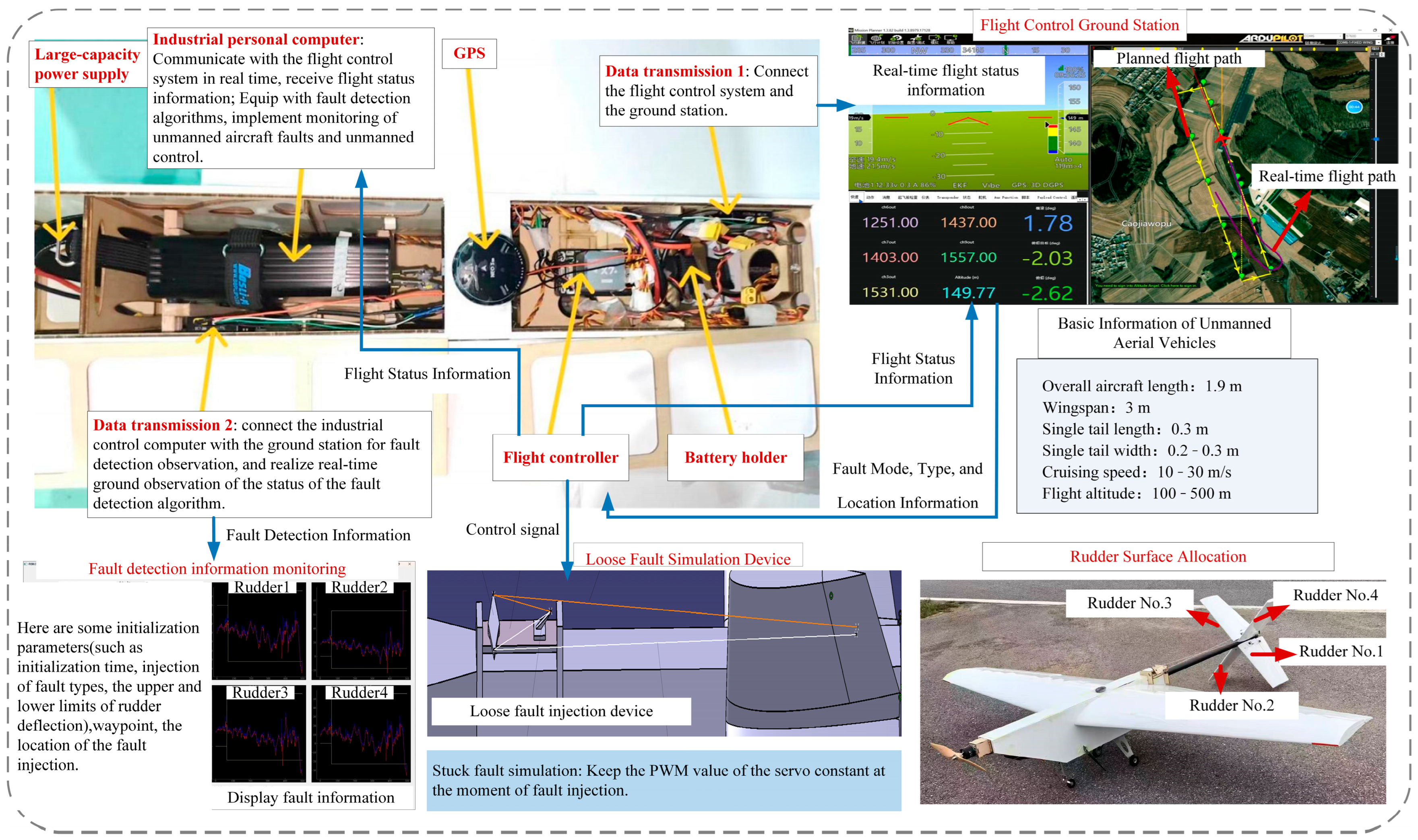
To evaluate the effectiveness of the proposed method, a comprehensive flight test system was developed using a FW-UAV, as illustrated in Figure 8. The experimental setup is divided into two primary components: the airborne system and the ground system, interconnected through a digital radio link for seamless communication. The airborne system comprises the fixed-wing UAV, an industrial computer, a flight controller, and a fault simulation device, enabling real-time data collection and fault injection during flight. On the ground, the system includes a fault monitoring station and a flight control ground station, which together facilitate real-time monitoring, data analysis, and operational control. This integrated setup provides a robust platform for validating the proposed actuator fault detection method under realistic flight conditions.

4.2. Flight Simulation and Data Selection

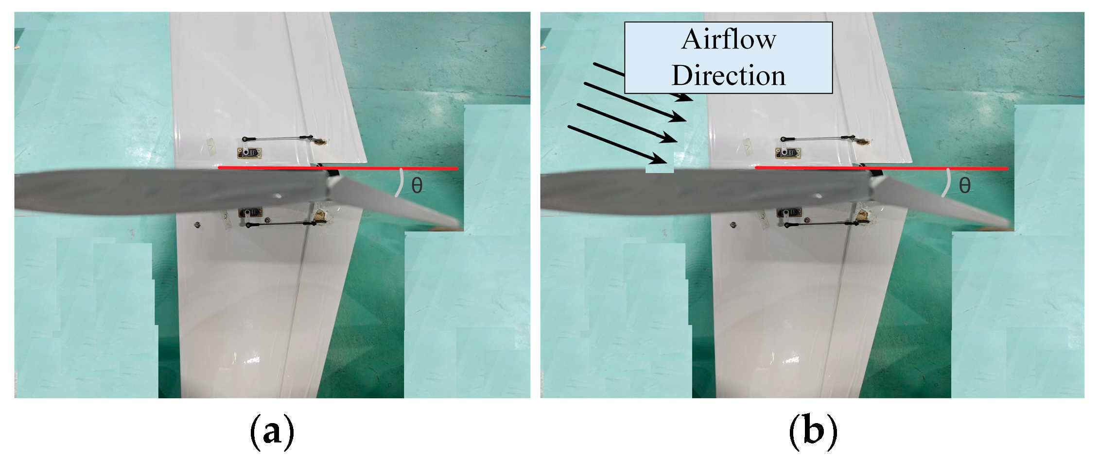
In the experiments, a fixed-wing UAV equipped with aerodynamic control surfaces was used, with two types of actuator faults (stuck and loose) simulated on the control surfaces, as illustrated in Figure 9. The stuck fault is characterized by the control surface being fixed at a certain angle, indicating a complete actuator failure, while the loose fault is characterized by the failure of hinge torque, causing the control surface to oscillate violently under airflow, indicative of a partial failure. These faults were implemented as follows: the stuck fault was realized by fixing the PWM signal of the servo at the moment of fault injection. For the loose fault, Rudder 1 was used as an example, employing two servos: one for deflection and another for controlling the tension of a cotton thread. Under normal conditions, the tensioning servo kept the thread taut to ensure proper rudder response; upon fault injection, the servo reversed to loosen the thread, triggering violent oscillations in Rudder 1.

To ensure the repeatability and reliability of fault simulation, calibration was conducted before formal testing. For the stuck fault, PWM signals were validated over multiple trials to remain within ±1% of the target value, ensuring consistent fault behavior. For the loose fault, the tension of the cotton thread was calibrated by adjusting the servo angle, with repeated tests confirming consistent oscillation patterns under airflow. Onboard sensors (IMU and GPS) were calibrated for accurate data collection: the IMU underwent static and dynamic calibration to correct for bias and temperature drift, while the GPS was calibrated against known reference points to minimize positioning errors. The ground station monitoring system was calibrated by validating telemetry data against known control inputs (e.g., pre-defined roll, pitch, yaw commands) and expected flight responses in a controlled test, ensuring accurate real-time fault recognition. These measures ensured consistent fault injection and detection, providing reliable data for DANN-based fault diagnosis across source and target domains.

The flight experiments were designed to evaluate the DANN-based MoE framework for actuator fault detection in UAVs, focusing on cross-domain fault diagnosis under diverse conditions. Conducted over 8 days from 29 July to 11 September 2024, at altitudes of 150–200 m, the real-world tests involved wind speeds categorized as ${\xi }_1$ (<1 m/s, no wind), ${\xi }_2$ (1–3 m/s, light wind), ${\xi }_3$ (3–5 m/s, middle wind), and ${\xi }_4$ (5–8 m/s strong wind), as detailed in

Table 1. Fault injection types and injection locations.

Fault Injection Types	Fault Injection Locations
stuck fault	Aileron 2, Aileron 3, Aileron 4
loose fault	Aileron 1

and

Table 2. Experiment dates, wind speed levels, and fault injection counts.

Wind Speed Level	Experiment Dates	Fault Injection Count
		Loose Fault	Stuck Fault
${\xi }_1$ (<1 m/s, no wind)	8.1, 9.11	81	200
${\xi }_2$ (1–3 m/s, light wind)	7.30, 8.2	56	162
${\xi }_3$ (3–5 m/s, middle wind)	8.31, 9.2	136	76
${\xi }_4$ (5–8 m/s, strong wind)	7.29, 9.1	57	208

, which lists test dates, wind speed levels, and the number of stuck and loose fault injections. Data covered normal, loose fault, and stuck fault states across typical flight scenarios like cruising and turning. Flight status data (acceleration, angular velocity, position) were collected at 100 Hz using IMU and GPS sensors. This setup, with varied wind speeds and scenarios, supported robust validation of the DANN-based fault detection framework in multi-task, cross-domain contexts.

The flight data collected from these experiments, including acceleration, angular velocity, and position, were subsequently processed to extract features for training and evaluating the DANN-based MoE framework. In summary, the experimental setup and calibration procedures ensured the collection of a comprehensive dataset under varied conditions, fully prepared for feature extraction, training, and evaluation in the next phase.

4.3. Experimental Data Processing

To enable efficient real-time processing, we selected 16 feature variables from over 40 recorded flight parameters, focusing on those most relevant to actuator fault detection based on prior research. These include attitude angles (roll, pitch, heading, yaw), angular rates (roll, pitch, yaw), airspeed, altitude, control inputs (roll, pitch, yaw, throttle), and control surface deflections (aileron, elevator, rudder). The selection focuses on variables particularly responsive to actuator faults, including conditions like stuck or loose control surfaces, which commonly lead to deviations in attitude or mismatches between intended and actual control actions. Previous studies have demonstrated the effectiveness of using attitude angles and control inputs for fault diagnosis in UAVs [27,28,29].

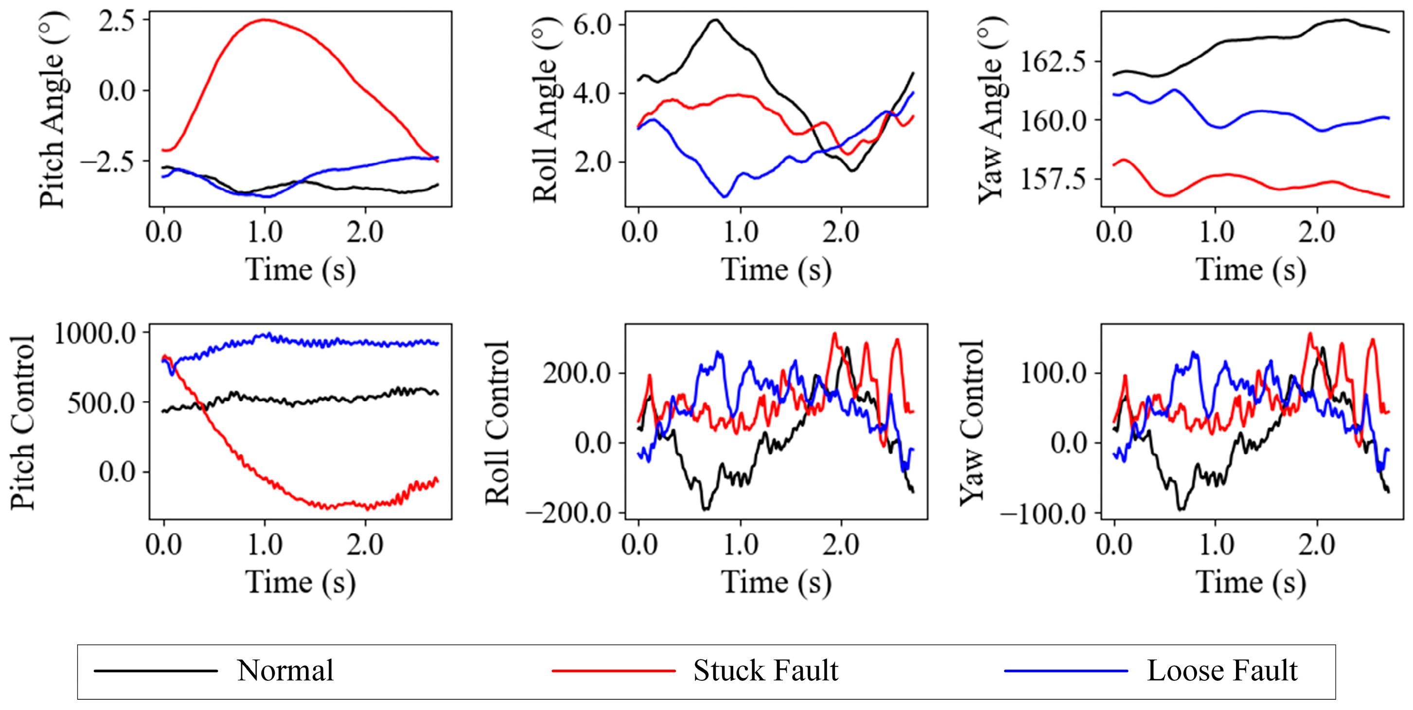
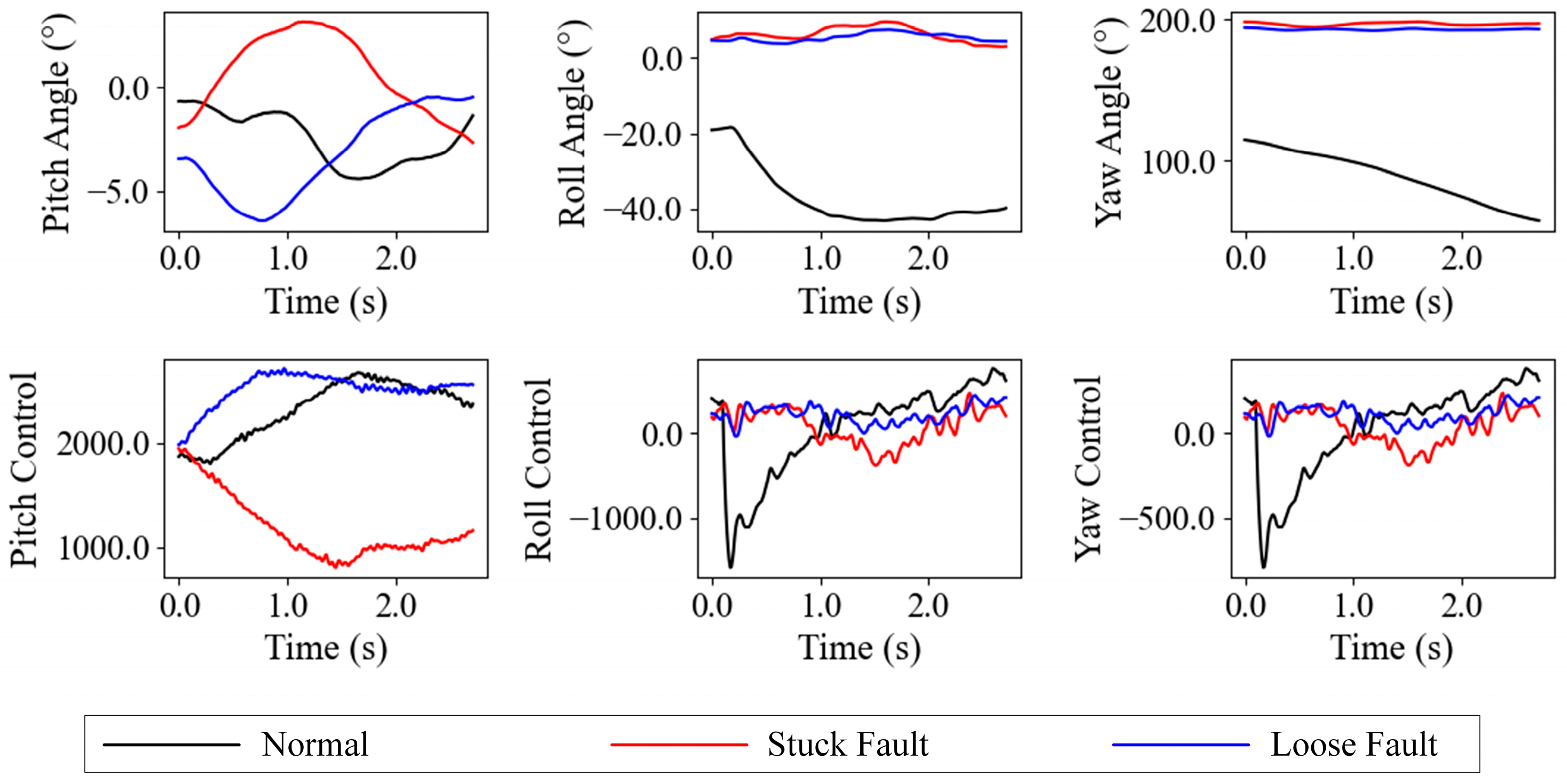
To highlight the dynamic effects of faults under varying environmental conditions, we visualize six key variables—pitch angle, roll angle, yaw angle, and their respective pitch control, roll control, and yaw control—under no-wind and strong wind conditions, as shown in Figure 10 and Figure 11. Figure 10 illustrates the flight parameters and control inputs under no-wind conditions, while Figure 11 depicts the same under strong wind conditions. Under strong wind conditions, the normal pitch angle may exhibit significant oscillations due to wind interference, closely resembling the oscillation patterns of a loose fault—for instance, the normal pitch angle fluctuations may mimic the high-frequency oscillations of a loose fault under strong wind influence, posing challenges for fault detection; stuck faults lead to a sustained deviation in the yaw angle. In no-wind conditions, the amplitude of oscillations and deviations caused by faults is reduced, making the distinction between normal and fault data more apparent. These state variables have different magnitudes or dimensions, so normalization is required to balance the influence of each parameter. The data for anomaly detection tasks may contain outliers that deviate significantly from the normal data, which could affect the normalization of normal data. To preserve the anomaly patterns after normalization, this approach uses robust normalization to process the data. The formal definition is as follows:

$$x^{*}={\displaystyle \frac{x-x_{media}}{x_{0.75}-x_{0.25}}},$$

(16)

where $x$ and $x^{*}$ represent the data before and after normalization, respectively. $x_{media}$ represents the median, $x_{0.75}$ is the 75th percentile, $x_{0.25}$ is the 25th percentile. After the input data is normalized through the neural network, the dimensions lose their significance.

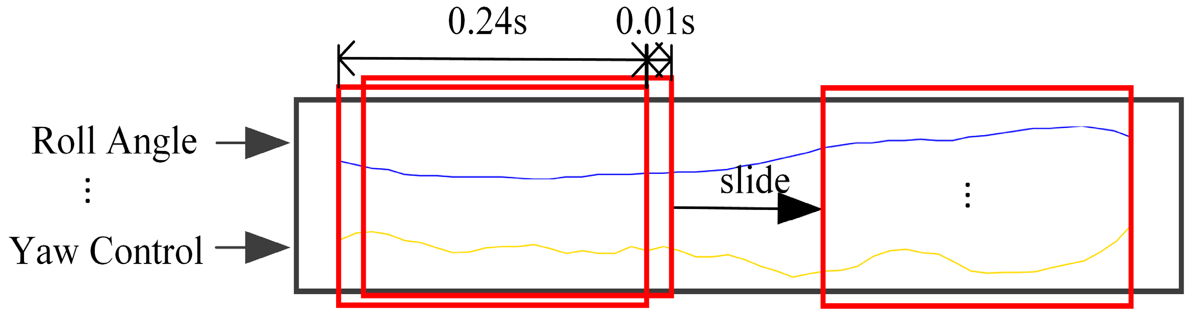
To ensure reproducibility and performance optimization, we configured key hyperparameters during the training process, which is detailed in Section 3.2.3. The training involves feeding UAV sensor data into the model, optimizing the combined loss (classification and domain adversarial) via gradient descent, and dynamically selecting experts using the noisy Top-K gating strategy. These hyperparameters are closely tied to data processing methods (e.g., sliding window size, as shown in Figure 12) and determine the model’s adaptability to diverse task scenarios.

Table 3. Hyperparameter settings.

Hyperparameter	Value	Rationale
$\lambda$	1.0	Balances fault classification and domain adaptation objectives to prevent over-alignment.
Window size	24	Captures dynamics of stuck and loose faults, determined through empirical testing to balance detection accuracy and computational efficiency.
Number of experts	3	Covers primary wind speed conditions, avoiding unnecessary computational complexity.
Top-K (Training)	2	Promotes collaborative learning across multimodal data, enhancing model robustness to environmental changes.
Top-K (Testing)	1	Optimizes inference speed for real-time fault detection needs.

summarizes the key hyperparameters, their values, and selection rationales.

The training process involves source domain data ${\left\{\right(x_t,y_t)\}}^n$ with labels and target domain data ${\left\{x_t\right\}}^{n^{\prime }}$. The testing data consist of target domain data ${\{(x_t,y_t)\}}^{n^{″}}$, where $n$, $n^{\prime }$, and $n^{″}$ represent the sample sizes of the source domain, the partially used target domain for training, and the remaining target domain, respectively.

According to the sliding window method for processing trajectory data mentioned above, the samples of the source domain and target domain are divided, and the resulting sample quantities are shown in

Table 4. Sample set information.

Task Scenario	Domain Category	Normal Sample Quantity	Fault Sample Quantity
1	Source domain: ${\xi }_1+{\xi }_2+{\xi }_3$	427,603	34,406
	Target domain: ${\xi }_4$	12,328	/
2	Source domain: ${\xi }_1+{\xi }_2+{\xi }_4$	539,293	56,778
	Target domain: ${\xi }_3$	15,235	/
3	Source domain: ${\xi }_1+{\xi }_3+{\xi }_4$	401,945	41,872
	Target domain: ${\xi }_2$	8328	/
4	Source domain: ${\xi }_2+{\xi }_3+{\xi }_4$	404,988	36,868
	Target domain: ${\xi }_1$	11,081	/

.

The accuracy of fault detection models is typically measured using the Fault Detection Rate (FDR) and False Alarm Rate (FAR) as evaluation metrics. FDR reflects the model’s ability to correctly detect fault samples, with a value closer to 1 indicating better performance. The FAR indicates the probability that the model incorrectly classifies normal samples as faults, with a value closer to 0 indicating better performance.

4.4. Experimental Results and Analysis

To verify the effectiveness of the method proposed in this paper, we conducted ablation experiments as well as comparative experiments with traditional methods.

4.4.1. Ablation Study

To verify the effectiveness of the proposed method, we conducted ablation experiments comparing traditional LSTM, a standalone DANN, and a DANN integrated within the MoE framework (DANN-MoE). In the experimental process, the MoE model activates two expert modules (Top-2) during the training phase to collaboratively optimize parameters and adapt to multimodal data distributions. In the testing phase, the strategy switches to Top-1, dynamically selecting the most suitable expert module based on the input, balancing inference efficiency and accuracy.

The experiments were conducted with four different random seed values for training, and detection results were calculated for each method. The statistical metrics of the experimental results, composed of the mean and standard deviation, are presented in Table 4. Ablation experiments demonstrate that DANN-MoE exhibits the best performance in the fault detection task, maintaining both a high FDR and a low FAR, significantly outperforming LSTM and standalone DANN methods. This indicates that the introduction of the MoE architecture effectively enhances the model’s detection accuracy and robustness.

Across the task scenarios evaluated in Table 4, DANN-MoE consistently outperforms standalone DANN and LSTM models. This improvement is driven by the DANN’s ability to handle environmental variations, reducing domain-specific biases, and the MoE’s capacity to differentiate multimodal fault patterns. In scenarios with mixed environmental fluctuations and fault types, the MoE’s expert networks reduce misclassifications by distinguishing subtle fault-induced anomalies from normal variations—a challenge where the DANN alone struggles. For instance, in the task ${\xi }_1+{\xi }_3+{\xi }_4 \to {\xi }_2$, the source domain contains a large number of samples under different wind speed conditions, enabling the model to comprehensively learn cross-domain features. Through the adversarial training mechanism of the DANN, the feature extractor G_f captures robust domain-invariant features, enhancing the target domain’s generalization ability and achieving higher accuracy and lower false alarm rates. The MoE’s Top-K gating strategy further optimizes the decision boundary by dynamically selecting the most suitable expert networks for multimodal data, reducing misclassifications.

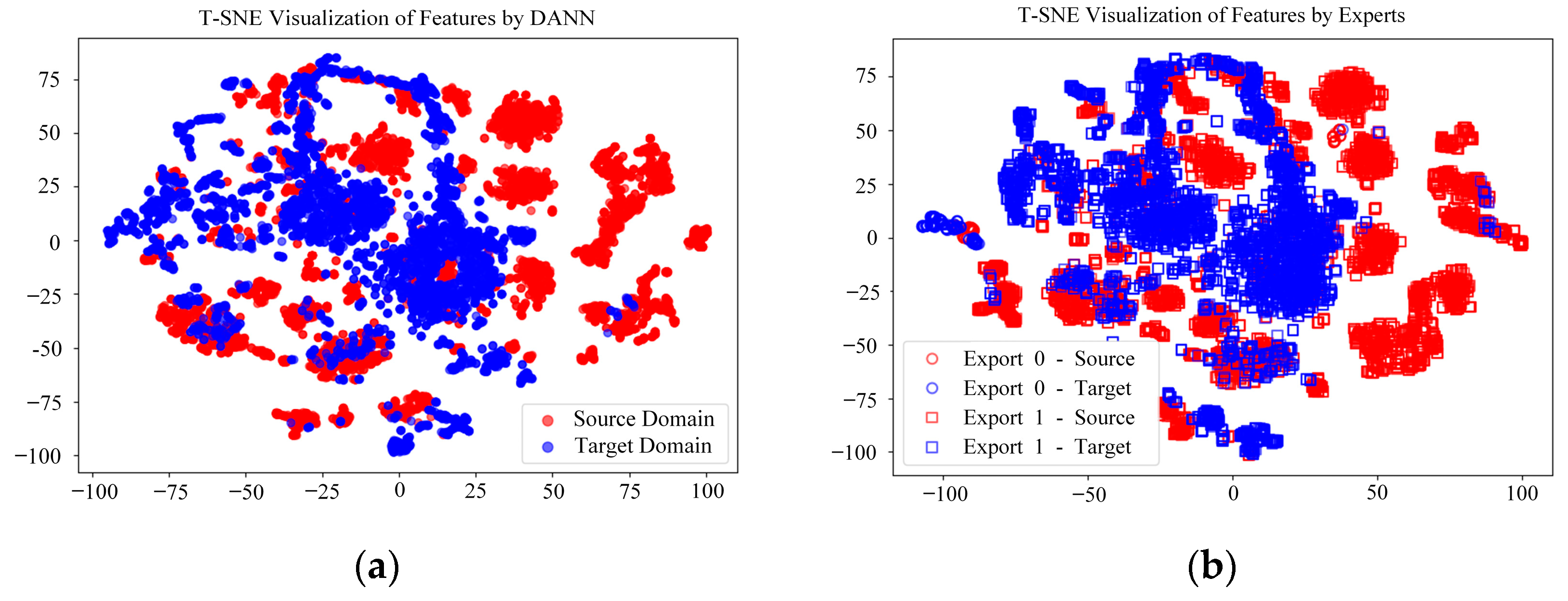
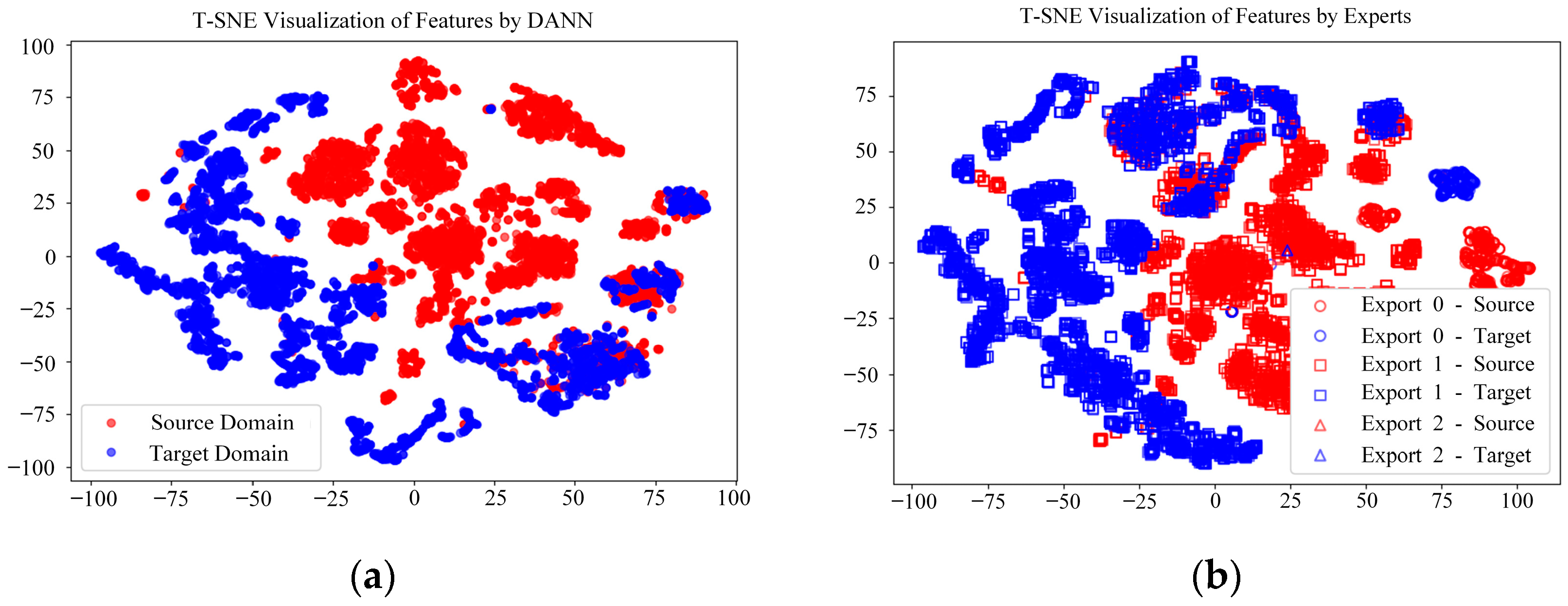
In our experiment, we set up a total of three experts in the DANN-MoE framework and activated the Top-1 expert during testing. To provide a more intuitive analysis, we visualize the features extracted by the feature extractor using t-distributed stochastic neighbor embedding (T-SNE) [30]. Figure 13a shows that, in Task Scenario 2, the features extracted by the standalone DANN exhibit a high degree of overlap between the target domain and the source domain, with blue points often overlaying red points. This indicates that the DANN successfully aligns the feature distributions of the source and target domains through domain-adversarial learning, achieving effective domain adaptation. Figure 13b presents the feature distribution of DANN-MoE, where the target and source domains’ features remain highly overlapped, while the expert division further enhances the model’s ability to handle different modal data. Similarly, Figure 14a,b illustrate the results for Task Scenario 3, where the DANN’s feature distribution also shows significant overlap between the target and source domains, and DANN-MoE, through expert division, maintains this alignment while further optimizing model performance. This high degree of feature overlap demonstrates the effectiveness of domain adaptation, and the expert division in DANN-MoE enhances the model’s adaptability to the target domain, as validated by the significant improvements in fault detection accuracy and robustness shown in

Table 5. Fault detection results.

Task Scenario	Method	FDR (%)	FAR (%)
1	LSTM	59.98 ± 2.13	51.79 ± 2.76
	DANN	75.59 ± 1.19	35.11 ± 2.07
	DANN+MOE	80.55 ± 1.15	26.40 ± 1.65
2	LSTM	83.72 ± 1.04	13.83 ± 2.10
	DANN	88.17 ± 1.52	10.46 ± 1.43
	DANN+MOE	93.26 ± 0.98	8.21 ± 0.97
3	LSTM	83.63 ± 1.54	15.68 ± 2.13
	DANN	90.63 ± 1.37	8.32 ± 1.12
	DANN+MOE	93.42 ± 1.16	6.21 ± 1.01
4	LSTM	82.74 ± 2.29	34.93 ± 1.89
	DANN	87.32 ± 1.37	14.28 ± 2.02
	DANN+MOE	90.91 ± 1.05	11.01 ± 1.17

.

Table 6. Comparison of computational resources and inference time.

Indicator	DANN	DANN-MoE	Relative Differences
Mean inference time (ms)	0.61	0.63	3.28%
Memory usage (GB)	0.96	1.07	11.46%

presents the inference time and memory usage of the DANN and DANN-MoE. DANN-MoE’s mean inference time increases by only 3.28% compared to DANN, ensuring real-time diagnostic capability. Regarding memory usage, DANN-MoE’s 1.07 GB is only 11.46% higher than the DANN’s 0.96 GB, remaining well below the 16 GB available on onboard computers. This method exhibits minimal increases in inference time and memory usage, verifying its efficiency and real-time diagnostic capability under limited computational resources.

4.4.2. Comparison to Other Methods

In this section, the proposed DANN-MoE model is compared with several established fault detection methods, including Support Vector Machine (SVM), Convolutional Neural Network (CNN), Deep Domain Confusion (DDC), and Multi-layer Maximum Mean Discrepancy (MMDA), as outlined in

Table 7. Information of various methods.

Methods	Domain Adaptation Methods	Details
SVM	None	Traditional machine learning method: support vector machine
CNN	None	Ordinary convolution neural network
DDC	MMD	An adaptative MMD criterion metric is added to the previous layer of the classifier
MMDA	MMD	Multilayer MMD domain adaptation

. These methods were evaluated across the same four task scenarios from Section 4.4.1, with each tested using four random seeds for consistency. The results, shown in

Table 8. Experimental results of different methods in different tasks.

Methods	Indicator	Task Scenario 1	Task Scenario 2	Task Scenario 3	Task Scenario 4
SVM	FDR (%)	58.89 ± 2.71	81.04 ± 2.11	83.76 ± 1.21	79.76 ± 1.48
	FAR (%)	50.65 ± 2.54	14.73 ± 1.64	14.43 ± 1.75	32.98 ± 2.62
CNN	FDR (%)	55.68 ± 1.30	79.68 ± 1.23	79.18 ± 1.15	75.92 ± 1.31
	FAR (%)	50.46 ± 1.63	16.54 ± 1.94	15.63 ± 2.32	35.65 ± 2.04
DDC	FDR (%)	73.23 ± 1.20	89.91 ± 1.43	87.28 ± 2.18	85.34 ± 1.52
	FAR (%)	33.17 ± 1.29	11.04 ± 2.35	14.57 ± 1.79	13.53 ± 2.17
MMDA	FDR (%)	75.46 ± 1.90	89.73 ± 1.68	89.18 ± 1.97	84.11 ± 1.72
	FAR (%)	39.61 ± 1.89	14.90 ± 1.75	10.84 ± 1.64	10.26 ± 1.06
LSTM	FDR (%)	59.98 ± 2.13	83.72 ± 1.04	83.63 ± 1.54	82.74 ± 2.29
	FAR (%)	51.79 ± 2.76	13.83 ± 2.10	15.68 ± 2.13	34.93 ± 1.89
DANN	FDR (%)	75.59 ± 1.19	88.17 ± 1.52	90.63 ± 1.37	87.32 ± 1.37
	FAR (%)	35.11 ± 2.07	10.46 ± 1.43	8.32 ± 1.12	14.28 ± 2.02
DANN-MoE (ours)	FDR (%)	80.55 ± 1.15	93.26 ± 0.98	93.42 ± 1.16	90.91 ± 1.21
	FAR (%)	26.40 ± 1.17	8.21 ± 0.97	6.21 ± 1.01	11.01 ± 1.05

, measure FDR and FAR, with all methods fine-tuned for a fair comparison.

DANN-MoE consistently outperforms these baselines. For example, in Task Scenario 3, it achieves an FDR of 93.42% and an FAR of 6.21%, surpassing SVM’s 83.76% FDR and 14.43% FAR, and CNN’s 79.18% FDR and 15.63% FAR. It also beats domain adaptation methods like DDC (87.28% FDR) and MMDA (89.18% FDR), while keeping the FAR lower. This shows its strength in accurately detecting faults and minimizing false alarms across varied conditions.

Traditional methods like SVM and CNN, which do not adapt to shifting data distributions, struggle in complex scenarios. In Task Scenario 1, their FARs reach around 50%, while DANN-MoE reduces this to 26.40%. This gap highlights its ability to handle environmental changes effectively. However, compared to a standalone DANN (35.11% FAR), the improvement is smaller, possibly due to challenges with the strong winds in ${\xi }_4$.

When compared to CNN and SVM, which rely on fixed features or large labeled datasets, DANN-MoE proves more adaptable and robust, especially in changing environments. The results show that methods like SVM and CNN are less effective at handling diverse tasks, while the DANN aligns features across scenarios, and the MoE refines decisions with specialized experts. This combination leads to better overall performance.

An interesting observation can be made in Task Scenario 1, where the DANN-MoE model shows a relatively lower FAR reduction compared to other task scenarios. This could be attributed to the greater difficulty in adapting to this specific scenario, possibly due to significant differences between this dataset and other datasets. The DANN framework, while effective in aligning features across different tasks, may face challenges in scenarios with large data distribution discrepancies. This is likely due to the flight data from ${\xi }_4$ exhibiting a substantial distribution difference compared to other wind speed levels, which complicates the feature extractor’s ability to align the source and target domain distributions.

Overall, the findings underline the effectiveness of the DANN-MoE approach in UAV actuator fault detection. By combining domain adaptation and expert-based decision-making, our method not only improves detection accuracy but also significantly reduces false alarms, making it a more reliable solution for real-world applications.

5. Conclusions

This study introduces a fault detection method for UAVs by combining a DANN with an MoE framework, effectively addressing data distribution shifts and adaptability challenges in diverse flight environments. The DANN component ensures robust generalization by extracting domain-invariant features, while the MoE enhances performance through dynamic handling of multimodal data. Flight experiments across various task scenarios demonstrate that the proposed method consistently outperforms traditional approaches like LSTM and a standalone DANN, achieving higher fault detection accuracy and lower false alarm rates. It also maintains computational efficiency, making it suitable for resource-constrained UAV systems. Future research could explore applying this method to other UAV types, such as multirotor drones, optimizing computational efficiency further, and addressing more complex environmental conditions with larger distribution shifts.