Adaptive Impact-Time-Control Cooperative Guidance Law for UAVs Under Time-Varying Velocity Based on Reinforcement Learning

Abstract

In this study, an adaptive impact-time-control cooperative guidance law based on deep reinforcement learning considering field-of-view (FOV) constraints is proposed for high-speed UAVs with time-varying velocity. Firstly, a reinforcement learning framework for the high-speed UAVs’ guidance problem is established. The optimization objective is to maximize the impact velocity; and the constraints for impact time, dive attacking, and FOV are considered simultaneously. The time-to-go estimation method is improved so that it can be applied to high-speed UAVs with time-varying velocity. Then, in order to improve the applicability and robustness of the agent, environmental uncertainties, including aerodynamic parameter errors, observation noise, and target random maneuvers, are incorporated into the training process. Furthermore, inspired by the ${\mathrm{RL}}^2$ algorithm, the recurrent layer is introduced into both the policy and value network. In this way, the agent can automatically adapt to different mission scenarios by updating the hidden states of the recurrent layer. In addition, a compound reward function is designed to train the agent to satisfy the requirements of impact-time control and dive attack simultaneously. Finally, the effectiveness and robustness of the proposed guidance law are validated through numerical simulations conducted across a wide range of scenarios.

1. Introduction

As mission scenarios for multiple cross-domain UAVs have become increasingly complex, the requirements of UAV guidance systems have also become more sophisticated [1,2,3]. The implementation of saturation attacks through impact-time-control guidance (ITCG) can effectively improve the penetration probability of cross-domain UAVs when facing a defense system [1]. It is therefore evident that impact-time-control guidance has become a crucial aspect of guidance technology.

The existing studies on ITCG could be divided into two categories. The first category is based on the biased proportional navigation guide (BPNG) law [4,5], which consists of the PNG law and a bias term for correcting the arrival time error. The second category is based on modern advanced control theories, including stability theory [6,7], sliding-mode variable structures [8,9,10], and backstepping control [11,12,13]. However, the BPNG laws are unable to guarantee robustness in complex environments, while guidance laws based on modern advanced control theories usually require accurate estimation of time-to-go.

To prevent high-speed UAVs from losing track of the target, the seeker’s FOV limits must be considered. There are several approaches to dealing with FOV constraints, one of which is to use compound guidance laws consisting of two or more phases [14,15,16]. However, the discontinuous guidance command at the moment of switching guidance laws may result in undesired transient responses. Another approach to addressing the FOV constraints is to shape the trajectory of the look angle [17,18,19], then the guidance commands are generated by designing reference-trajectory tracking control laws. Other approaches such as optimal control theory [2,20] or nonlinear control theory [21,22] have also been used to address FOV constraints. Although there have been many studies on ITCG and FOV constraints, existing methods are difficult to apply directly to high-speed UAVs with time-varying velocity. On the other hand, the coupling effects between the longitudinal and lateral channel in three-dimensional (3D) space cannot be ignored.

In recent years, computational guidance algorithms have received increasing attention due to the rapid development of embedded computing capabilities. The authors in ref. [23] proposed a guidance law with terminal time and impact angle constraints by employing model predictive static programming (MPSP). Similarly, the authors in ref. [24] proposed a guidance law for vehicle guidance with state and input constraints by using model predictive convex programming (MPCP) to solve guidance commands. Although these approaches can obtain optimal or suboptimal guidance commands online, a poor initial solution may result in difficulties in achieving convergence during the computational process [25].

Deep reinforcement learning (DRL) techniques have undergone substantial advancements and progress in recent years and have demonstrated exceptional performance in decision-making tasks involving high-dimensional data [26]. However, previous studies have focused on DRL applications in intelligent control, with few studies focusing on guidance problems in aerospace. To solve the missile guidance problem in the terminal flight phase, the DDPG algorithm was used to train the agent [27]. The authors in ref. [28] proposed an ITCG law with FOV constraints, where the guidance gain was obtained by DDPG. Similarly, the authors in ref. [29] proposed an impact-angle-control guidance (IACG) law based on BPNG, where the bias term was obtained by a series of training processes. Ref. [30] proposed an terminal flight guidance law for hypersonic gliding vehicles employing the meta-reinforcement learning technique. In Ref. [31], the authors proposed an ITCG algorithm based on a general prediction–correction framework; the method employed a DNN to predict the time-to-go, then the correction commands were learned by using proximal policy optimization (PPO). The author in [32] developed a cooperative interception guidance law for multiple missiles by using the action-enhanced multi-agent deep deterministic policy gradient (EA-MADDPG) algorithm. However, the FOV constraints and velocity with time-varying conditions were not considered. Although the agent training and learning process may be time-consuming when utilizing DRL methods, acquiring guidance commands after deployment requires only computing the output of the neural network.

Although many guidance laws have been developed so far, there are still challenges that need to be addressed through further research to achieve practical implementation. First, the majority of existing studies on ITCG are developed using ideal kinematic assumptions. However, the applicability of these assumptions needs to be carefully examined, especially in the context of UAVs with time-varying velocity and three-dimensional pursuit scenarios. Second, most existing ITCG laws require an accurate estimated value of the time-to-go; therefore, the accuracy of the time-to-go estimation could directly affect the performance of ITCG laws. Third, the application of the DRL method to the development of guidance laws still presents certain limitations that require further attention. These include the development of guidance laws for high-speed UAVs with time-varying velocity and the consideration of FOV constraints on the guidance process.

Based on the above discussion, this study proposes an adaptive ITCG law with FOV constraints for high-speed UAVs with time-varying velocity. The objective is to achieve a cooperative dive attack and maximize impact velocity. To this end, the high-speed UAVs’ guidance problem is first reconstructed in the DRL framework. Furthermore, uncertainties of the environment are considered, including random perturbation biases in aerodynamic coefficients and atmospheric density, random maneuvers of the target, and observation noise. We also impose path constraints on the FOV angle and overload. Finally, a compound reward function is proposed to compensate for guide accuracy, energy consumption, and impact-time error. The state-of-the-art DRL algorithm PPO is used to train the agent that maps the observations to guidance commands. Inspired by the ${\mathrm{RL}}^2$ algorithm [33], a gated recurrent unit (GRU) layer is introduced into the policy network. This enables the well-trained agent to rapidly adapt to the different environment and tasks by updating the hidden state of the GRU layer during deployment.

The contributions of this paper are summarized below. Firstly, the ITCG law for high-speed UAVs with time-varying velocity is developed on the basis of DRL techniques. The objective of this study was to achieve terminal time control for high-speed UAVs with time-varying velocity and to enable dive attacks; a compound reward function is proposed that consists of a positive reward and negative penalty to ensure the high-speed UAV arrives at the target while continuously correcting the arrival time. Secondly, a straightforward but effective time-to-go estimation approach for time-varying velocity is proposed, which has higher accuracy than the analytical formula prediction method. In addition, to improve the applicability of the guidance law in practical application scenarios, FOV constraints and overload constraints are considered. Third, inspired by the ${\mathrm{RL}}^2$ algorithm [33], the gated recurrent unit (GRU) layers are introduced into the policy network and the value network to achieve rapid adaptation to different tasks by continuously updating the hidden states of the GRU layers.

This paper is organized as follows: Section 2 briefly reviews the PPO algorithm. Section 3 formulates the guidance problem for the UAV. Section 4 details the proposed guidance law. Section 5 shows the results of the numerical simulations. Finally, Section 6 provides the conclusion.

2. Preliminary

The proximal policy optimization algorithm (PPO) [34] is recognized for its benchmark performance in complex control tasks. It implements a two-stream neural network structure: the actor network is used to generate the action for the observation at the current time step, and the critic network is used to approximate the state value function, which evaluates the value of the current state.

Let $\theta ,w$ denote the parameters of the actor network and the critic network, respectively. The probability ratio of the new policy ${\pi }_{\theta }$ to the old policy ${\pi }_{{\theta }^{-}}$ is calculated as follows:

$$p_t\left(\theta \right)={\displaystyle \frac{{\pi }_{\theta }\left(a_t\right|s_t)}{{\pi }_{{\theta }^{-}}\left(a_t\right|s_t)}}$$

(1)

The optimization objective of the PPO algorithm is to maximize the objective function as follows:

$$J\left(\theta \right)=\mathbb{E}\left(min(p_t\left(\theta \right),\mathrm{clip}(p_t\left(\theta \right),1-ϵ,1+ϵ)){\widehat{A}}_t\right)$$

(2)

where $ϵ$ represents the clip coefficient, and ${\widehat{A}}_k$ represents the estimated value of the advantage function at time step k, which can be obtained as follows:

$${\widehat{A}}_t=\left[\sum _{k=t}^T{\gamma }^k{r}_{t+k}\right]-V_w^{\pi }\left(s_t\right)$$

(3)

where the state value function $V_w^{\pi }$ is updated by minimizing the loss function as follows:

$$L\left(w\right)=\sum _{i=1}^{\left|D\right|}{\left(V_w^{\pi }\left(s_t\right)-\left[\sum _{k=t}^T{\gamma }^k{r}_{t+k}\right]\right)}^2$$

(4)

where $\left|D\right|$ represents the total number of collected data. Then, the parameters $\theta$ can be updated by maximizing the objective function $J\left(\theta \right)$, and the parameters w can be minimized using the loss function $L\left(w\right)$, that is,

$${\theta }^{+}={\theta }^{-}+{\alpha }_{\theta }{\nabla }_{\theta }{J\left(\theta \right)|}_{\theta ={\theta }^{-}}$$

(5)

$$w^{+}=w^{-}-{\alpha }_w{\nabla }_w{L\left(w\right)|}_{w=w^{-}}$$

(6)

where ${\alpha }_{\theta }$ and ${\alpha }_w$ denote the learning rates for the actor network ${\pi }_{\theta }\left(a_t\right|s_t)$ and the critic network $V_w^{\pi }\left(s_t\right)$, respectively.

3. Problem Statement

As part of the system design, we established a local geodetic reference frame (Figure 1) following the North–East–Down (NED) convention: the x-axis aligned with true north, the z-axis pointed eastward, and the y-axis completed the orthogonal right-handed coordinate system. The following foundational assumptions were introduced to formulate the problem.

Assumption 1. 

The vehicle adopts a bank-to-turn (BTT) control scheme, that is, the side slip angle β of the high-speed UAV is always steered to be zero.

Assumption 2. 

The high-speed UAV and target are treated as mass points.

Assumption 3. 

The target’s velocity is much smaller than that of the high-speed UAV.

This paper focused primarily on the guidance problem of high-speed UAVs during the terminal flight phase; therefore, the effects of Earth’s curvature were neglected. Thus, according to Assumptions 1 and 2, the 3D motion equations of a high-speed UAV could be expressed as follows [35]:

$$\begin{array}{cc}\hfill {\dot{x}}_M& =V_{M}cos\gamma cos\psi \hfill \end{array}$$

(7a)

$$\begin{array}{cc}\hfill {\dot{y}}_M& =V_{M}sin\gamma \hfill \end{array}$$

(7b)

$$\begin{array}{cc}\hfill {\dot{z}}_M& =V_{M}cos\gamma sin\psi \hfill \end{array}$$

(7c)

$$\begin{array}{cc}\hfill {\dot{V}}_M& =-{\displaystyle \frac{D}{m}}-gsin\gamma \hfill \end{array}$$

(7d)

$$\begin{array}{cc}\hfill \dot{\gamma }& ={\displaystyle \frac{Lcos\sigma }{m{V}_M}}-{\displaystyle \frac{g}{V}}cos\gamma \hfill \end{array}$$

(7e)

$$\begin{array}{cc}\hfill \dot{\psi }& ={\displaystyle \frac{Lsin\sigma }{V_{M}cos\gamma }}\hfill \end{array}$$

(7f)

$$\begin{array}{cc}\hfill \dot{\alpha }& =\Delta \alpha \hfill \end{array}$$

(7g)

$$\begin{array}{cc}\hfill \dot{\sigma }& =\Delta \sigma \hfill \end{array}$$

(7h)

where $x_M,y_M,z_M$ represent the position coordinates of the vehicle, and $V_M$ denotes the velocity of the UAV. The definitions of other symbols are shown in Figure 1. The gravity acceleration $g=9.81{\mathrm{m}/\mathrm{s}}^2$. $\alpha$ and $\sigma$ represent the angle of attack and bank angle, respectively. The expressions of the aerodynamic lift and drag forces are as follows:

$$\begin{array}{cc}\hfill L& ={\displaystyle \frac{1}{2}}\rho V_M^2{S}_{ref}{C}_L\hfill \end{array}$$

(8a)

$$\begin{array}{cc}\hfill D& ={\displaystyle \frac{1}{2}}\rho V_M^2{S}_{ref}{C}_D\hfill \end{array}$$

(8b)

where $\rho$ denotes the atmospheric density, $S_{ref}$ represents the reference area, and $C_L$ and $C_D$ are the lift and drag coefficients.

In addition, the actuator delay was also considered, that is,

$$\begin{array}{cc}\hfill \dot{\Delta \alpha }& ={\displaystyle \frac{\Delta {\alpha }_c-\Delta \alpha }{{\tau }_a}}\hfill \end{array}$$

(9a)

$$\begin{array}{cc}\hfill \dot{\Delta \sigma }& ={\displaystyle \frac{\Delta {\sigma }_c-\Delta \sigma }{{\tau }_b}}\hfill \end{array}$$

(9b)

where ${\tau }_a$ and ${\tau }_b$ are the actuator time constants, $\Delta \alpha$ and $\Delta \sigma$ are the actual angular rates, and $\Delta {\alpha }_c$ and $\Delta {\sigma }_c$ are the command angular rates.

Consider a maneuvering target on the ground with the following motion equations:

$$\begin{array}{cc}\hfill {\dot{\mathit{r}}}_T& ={\mathit{v}}_T\hfill \end{array}$$

(10a)

$$\begin{array}{cc}\hfill {\dot{\mathit{v}}}_T& ={\mathit{a}}_T\hfill \end{array}$$

(10b)

where ${\mathit{r}}_T,{\mathit{v}}_T,$ and ${\mathit{a}}_T$ denote the position, velocity, and acceleration vector of the target, respectively. Because the target only maneuvers on the ground, $y_T=v_{yT}=a_{yT}=0$. Moreover, the amplitude of the velocity and acceleration of the target need to satisfy the following limits:

$$\begin{array}{cc}\hfill {\mathit{r}}_T\left(t_0\right)& ={[0,0,0]}^T\hfill \end{array}$$

(11a)

$$\begin{array}{cc}\hfill \parallel {\mathit{v}}_T\parallel & \le V_{T_{max}}\hfill \end{array}$$

(11b)

$$\begin{array}{cc}\hfill \parallel {\mathit{a}}_T\parallel & \le a_{T_{max}}\hfill \end{array}$$

(11c)

Let ${\mathit{r}}_M={\left[x_M,y_M,z_M\right]}^T$ denote the position vector of the vehicle and ${\mathit{r}}_{TM}$ denote the vector from the vehicle to the target; then, the elevation angle ${\theta }_L$ and azimuth angle ${\psi }_L$ of the line-of-sight (LOS) vector are defined as follows:

$$\begin{array}{cc}\hfill {\theta }_L& =arcsin{\displaystyle \frac{y_T-y_M}{\parallel {\mathit{r}}_{TM}\parallel }}\hfill \end{array}$$

(12a)

$$\begin{array}{cc}\hfill {\psi }_L& =arctan2(z_T-z_M,x_T-x_M)\hfill \end{array}$$

(12b)

where ${\mathit{r}}_{TM}={\mathit{r}}_T-{\mathit{r}}_M$, and $arctan2(·,·)$ denotes the four-quadrant inverse tangent function. Taking the time derivative of ${\theta }_L,{\psi }_L$ and combining it with Equation (7a–h), we can obtain

$$\begin{array}{cc}\hfill {\dot{\theta }}_L& ={\displaystyle \frac{V_{M}cos\gamma sin({\psi }_L-\psi )}{S_{TM}}}\hfill \end{array}$$

(13a)

$$\begin{array}{cc}\hfill {\dot{\psi }}_L& =-{\displaystyle \frac{V_M\left(cos{\theta }_{L}sin\gamma -sin{\theta }_{L}cos\gamma cos({\psi }_L-\psi )\right)}{\parallel {\mathit{r}}_{TM}\parallel }}\hfill \end{array}$$

(13b)

where $S_{TM}=\sqrt{{(x_T-x_M)}^2+{(z_T-z_M)}^2}$ represents the length of the projection of the LOS vector in the horizontal plane.

In addition, the leading angle $\eta$ of the vehicle, which represents the angle between the LOS vector and the velocity vector of the vehicle, can be calculated as follows:

$$\eta =arccos\left({\displaystyle \frac{{\mathit{r}}_{TM}^T·{\mathit{v}}_M}{\parallel {\mathit{r}}_{TM}\parallel ·\parallel {\mathit{v}}_M\parallel }}\right)$$

(14)

The primary goal of the designed guidance law is to achieve the following final conditions:

$$|t_f-T_d|\le {ϵ}_{{\delta }_t}$$

(15)

$$\parallel {\mathit{r}}_M\left(t_f\right)-{\mathit{r}}_T\left(t_f\right)\parallel \le {ϵ}_r$$

(16)

$${\gamma }_f\le {\gamma }_{dive}$$

(17)

where $t_f$ and $T_d$ represent the final time and the desired final time, respectively. ${\gamma }_{dive}$ represents the minimum path angle required for dive attacking.

Moreover, the path constraints should also be considered, such as the overload constraints and FOV constraints, that is,

$${\displaystyle \frac{\sqrt{L^2+D^2}}{mg}}\le n_{max}$$

(18)

$$|\eta \left(t\right)+\alpha \left(t\right)|\le FO{V}_{max},\forall t\le t_f$$

(19)

where $n_{max}$ and $FO{V}_{max}$ denote the allowable maximum limit of the overload and FOV angle of vehicle, respectively.

It should be noted that the majority of existing studies [19,20] express the FOV constraint in the form of $\left|\eta \left(t\right)\right|\le FO{V}_{max}$. This is due to the fact that these studies employ the small-angle-of-attack assumption, by which the angle of attack is regarded as being approximately zero. However, in reality, the vehicle’s FOV angle is equal to the sum of the angle of attack and the leading angle (as illustrated in Figure 2), so we expressed the FOV constraints in the form of Equation (19).

Our objective was for the velocity of the vehicle to be as large as possible when it reached the target. Consequently, the designation of the guidance law was reduced to solving the following constrained optimization formulation:

$$min-V_M\left(t_f\right)$$

(20)

s.t.    (7), (15)–(19).

4. Method

This section presents a description of the guidance problem within the context of the DRL framework, together with an optimization of the guidance policy through the application of the PPO algorithm. The representative images in Figure 3 illustrate the reinforcement learning guidance framework employed in this study, where the IMU is the inertial measurement unit. The agent generates acceleration commands according to the observation information, and then the autopilot generates the angle of attack and bank angle change rate commands based on the acceleration command.

4.1. Observation Space and Action Space

For the guidance and control problems, the observation vector must fully describe the information about the relative state of the vehicle and target. Therefore, the observation vector was designed as follows:

$$\widetilde{{\mathit{o}}_t}={\left[\parallel {\mathit{r}}_{TM}\parallel ,\lambda ,V_M,{\dot{\theta }}_L,{\dot{\psi }}_L,{\widehat{t}}_{go},{\delta }_t,{\delta }_{\gamma }\right]}^T$$

(21)

where $\lambda ={\displaystyle \frac{{\mathit{r}}_{TM}}{\parallel {\mathit{r}}_{TM}\parallel }}$ denotes the LOS uni vector, ${\widehat{t}}_{go}$ denotes the estimated value of the time-to-go $t_{go}$, ${\delta }_t=t+{\widehat{t}}_{go}-T_d$ is the estimated arrival time error, and ${\delta }_{\gamma }={\displaystyle \frac{\pi }{2}}-{\theta }_L$. Moreover, the observation noise was considered, that is,

$${\mathit{o}}_t={\tilde{\mathit{o}}}_t·\mathcal{N}(1.0,{\epsilon }_{obs},n)$$

(22)

where $\mathcal{N}(1.0,{\epsilon }_{obs},n)$ denotes the n-dimensional independent Gaussian distributed random variables with mean 1.0 and standard deviation ${\epsilon }_{obs}$, and n is the dimension of the observation.

The majority of existing time-to-go estimation methods employ constant velocity and PNG guidance assumptions. However, the velocity is not constant during the terminal flight phase, and the guidance methods used do not necessarily adhere to the principles of PNG. Therefore, existing time-to-go estimation methods cannot be applied directly in vehicles with time-varying velocity. For this reason, we propose a straightforward but effective iterative approach to estimate the time-to-go. First, the initial guess for the remaining flight time estimate can be expressed as:

$${\widehat{t}}_{go}={\displaystyle \frac{\parallel {\mathit{r}}_{TM}\parallel }{\parallel {\dot{\mathit{r}}}_{TM}\parallel }}\approx {\displaystyle \frac{\parallel {\mathit{r}}_{TM}\parallel }{V_{M}cos\eta }}$$

(23)

Here, we utilized Assumption 3, as $V_T\ll V_M$, and thus $V_{MT}=V_M-V_T\approx V_M$. Based on the assumption that the derivative of the vehicle’s velocity with respect to time is constant, the predicted value of the terminal velocity can be calculated as follows:

$$V_f=V_M-{\dot{V}}_M{\widehat{t}}_{go}$$

(24)

It is important to note that, since the deviations in aerodynamic parameters and atmospheric density cannot be determined in advance, it is not feasible to calculate ${\dot{V}}_M$ using Equation (7d) in practice. However, in real-world applications, ${\dot{V}}_M$ can be directly obtained from the output of an accelerometer.

Then, the average velocity over the entire flight process can be obtained using the following equation:

$$V_{ave}={\displaystyle \frac{V_M+V_f}{2}}$$

(25)

Therefore, $V_M$ in Equation (23) can be replaced with the average velocity $V_{ave}$, thereby obtaining a new estimate for the time-to-go, expressed as

$${\widehat{t}}_{go}^{new}={\displaystyle \frac{\parallel {\mathit{r}}_{TM}\parallel }{V_{ave}cos\eta }}$$

(26)

In general, ${\widehat{t}}_{go}^{new}$ is not directly equal to ${\widehat{t}}_{go}$. However, after a few iterations of the above process, the estimate of time-to-go ${\widehat{t}}_{go}$ converges quickly.

It is worth noting that in the above analysis, we implicitly used two assumptions: ${\dot{V}}_M$ is constant, and the leading angle $\eta$ is also constant. These assumptions may introduce errors in the final estimate. However, the estimation error of the time-to-go will also gradually converge to zero as the distance between the UAV and the target continues to decrease. The time-to-go estimation approach is shown in Algorithm 1.

Algorithm 1 Improved time-to-go estimation algorithm

Input: Error tolerance ${ϵ}_e$, maximum number of iterations $N_{iter}$, distance $\parallel {\mathit{r}}_{TM}\parallel$, leading angle $\eta$, velocity $V_M$ and the rate of change in velocity ${\dot{V}}_M$ Output: Estimated value of time-to-go ${\widehat{t}}_{go}$ 1: Let $k=0$, ${\widehat{t}}_{go}^{old}={\displaystyle \frac{\parallel {\mathit{r}}_{TM}\parallel }{V_{M}cos\eta }}$ 2: while  $|{\widehat{t}}_{go}^{old}-{\widehat{t}}_{go}^{new}|>{ϵ}_e$  do 3:     Let ${\widehat{t}}_{go}^{old}={\widehat{t}}_{go}^{new}$ 4:     Estimated the final velocity of vehicle $V_f=V_M+{\dot{V}}_M{\widehat{t}}_{go}^{old}$ 5:     Obtain the mean velocity $V_{ave}={\displaystyle \frac{V_M+V_f}{2}}$ 6:     Obtain the new estimated value of time-to-go ${\widehat{t}}_{go}^{new}={\displaystyle \frac{\parallel {\mathit{r}}_{TM}\parallel }{V_{ave}cos\eta }}$ 7:      $k=k+1$ 8:      if $k\ge N_{iter}$ then 9:          Break 10:    end if 11: end while 12: return The estimated value of time-to-go ${\widehat{t}}_{go}^{new}$.

The proposed time-to-go estimation algorithm has the following advantages: First, it does not rely on any specific guidance law, making it applicable to a broader range of scenarios. In contrast, traditional analytical prediction formulas [8,9,10] can only predict the remaining flight time for trajectories derived from PNG. Second, compared to numerical integration methods, the proposed method benefits from its simple iterative process, offering superior real-time performance.

To avoid the excessive overload of the vehicle during flight, the action space was formed as an acceleration command, that is,

$${\mathit{a}}_t={\left[a_{yc},a_{zc}\right]}^T$$

(27)

where $a_{yc}$ and $a_{zc}$ are the required acceleration of the vehicle in the horizontal and vertical planes, respectively.

There are two principal reasons for adopting the acceleration command as the action. Firstly, the overload of the vehicle can be easily made to satisfy the constraints by applying a clip operation to the output of the policy $\pi \left({\mathit{o}}_t\right)$. Secondly, although taking the command angular rates $\left[\Delta \alpha ,\Delta \sigma \right]$ as action is an end-to-end solution, which makes the problem formulation more concise, it may prove challenging in terms of achieving convergence on the policy of the agent.

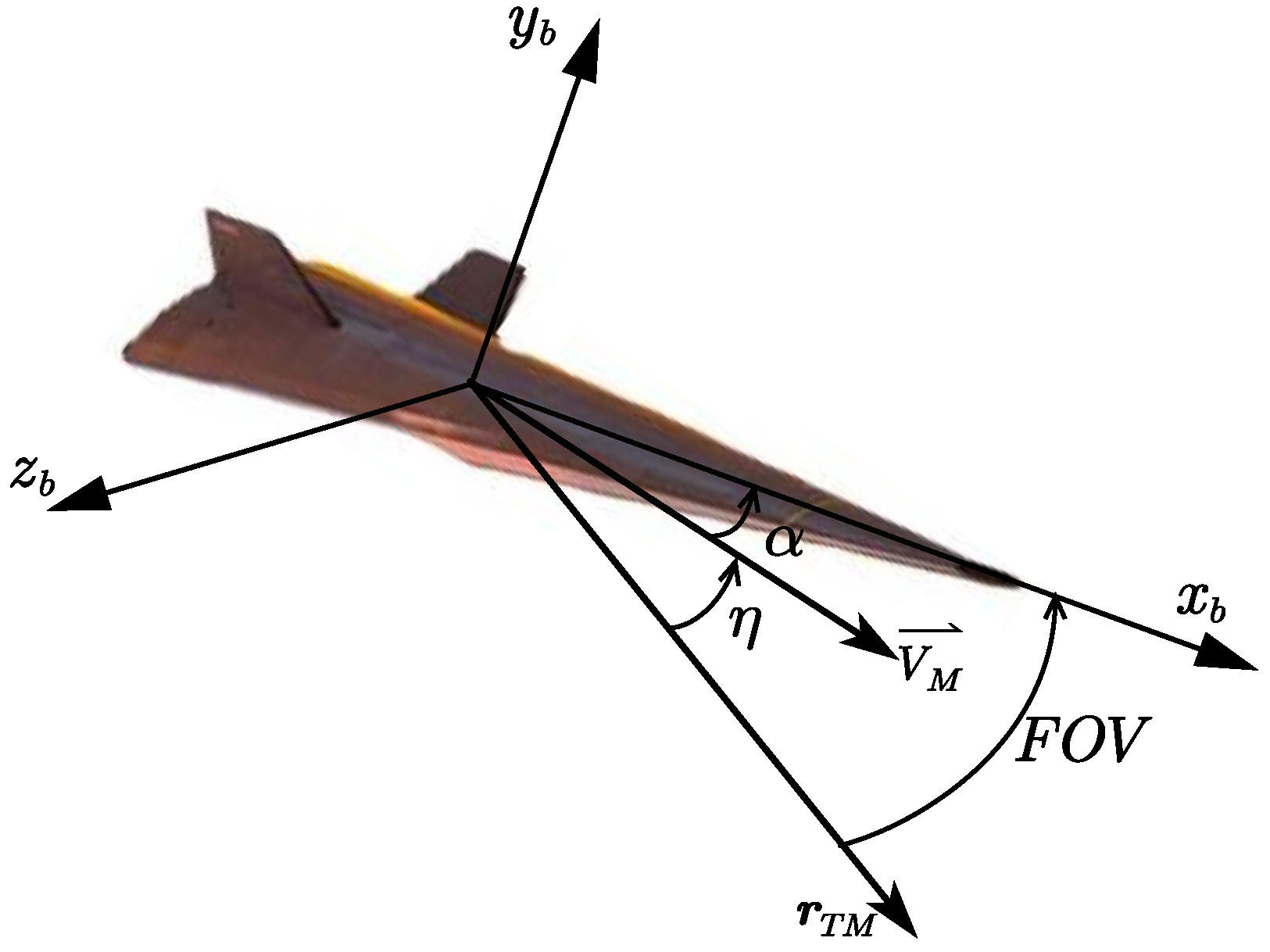
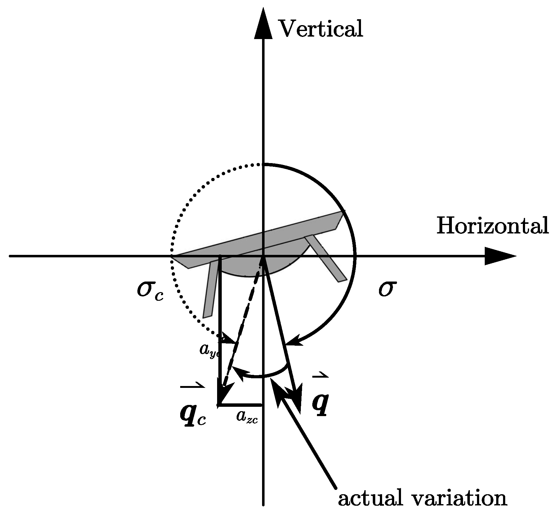
Although a method for calculating the angle of attack and bank angle commands was proposed in ref. [35], applying that method implies that when the sign of the required lift changes, the sign of the bank angle must also change accordingly. When the sign of the bank angle change occurs for larger orders of magnitude of the bank angle, it leads to the occurrence of undesired transient processes. To circumvent this challenging problem, we adopted an unlimited bank angle scheme which was employed in [12] (as illustrated in Figure 4). Consequently, a simple and effective computational approach is given.

Based on the action of the agent, the commands ${\alpha }_c$ can be obtained by solving the following equation:

$${\alpha }_c=\underset{{\alpha }_l\le \alpha \le {\alpha }_u}{argmin}|L-L_d|$$

(28)

where ${\alpha }_l$ and ${\alpha }_u$ represent the minimum and maximum values of the vehicle’s angle of attack, respectively. $L_d$ denotes the required lift force, whose expressions are given by the following equations:

$$L_d=m\sqrt{{(a_{yc}+gcos\gamma )}^2+a_{zc}^2}$$

(29)

Equation (28) is essentially a single-variable root-finding problem. In this paper, the Newton–Raphson method was employed to solve Equation (28). However, alternative methods such as the secant method or Brent’s method can also achieve rapid solutions for Equation (28).

Then, the commanded bank angle ${\sigma }_c$ can be obtained by the following equation with the unlimited bank angle control scheme:

$${\sigma }_c=arctan2(a_{zc},a_{yc}+gcos\gamma )$$

(30)

Finally, the commanded angular rate can be obtained by the following equations

$$\begin{array}{c}\hfill \Delta {\alpha }_c=\mathrm{clip}\left({\displaystyle \frac{{\alpha }_c-{\alpha }_t}{\Delta t}},-\Delta {\alpha }_{max},\Delta {\alpha }_{max}\right)\end{array}$$

(31a)

$$\begin{array}{c}\hfill \Delta {\sigma }_c=\mathrm{clip}\left({\displaystyle \frac{{\sigma }_c-{\sigma }_t}{\Delta t}},-\Delta {\sigma }_{max},\Delta {\sigma }_{max}\right)\end{array}$$

(31b)

where $\Delta t$ is the guidance period.

The adoption of an unlimited bank angle control scheme is motivated by two primary reasons: First, to satisfy the requirement for dive attacks, the high-speed UAV must generate a negative lifting force. If the bank angle is restricted to the range $\left[-\pi /2,\pi /2\right]$, the negative lift force can only be achieved through the negative angles of attack. However, for non-axisymmetric high-speed UAVs, the aerodynamic effects of negative and positive angles of attack often differ significantly, which increases control complexity. Second, when the high-speed UAV approaches the target, oscillations in guidance commands inevitably occur. When the sign of the required lateral acceleration $a_{zc}$ changes, the unlimited bank angle control scheme allows the bank angle to adjust by a small magnitude. In contrast, if the bank angle is restricted to $\left[-\pi /2,\pi /2\right]$, a sign change in $a_{zc}$ would require large variations in the bank angle, severely compromising the flight stability of high-speed UAVs.

4.2. Reward Function and Termination Conditions

The most significant challenge in using DRL to address the UAV with time-varying velocity guidance problem is developing an effective reward function in a sparse reward environment. If the reward signal is given only if the vehicle arrives at the target and satisfies the process and terminal constraints, it is probable that, with a limited number of episodes, the policy of the agent may encounter difficulty in identifying and exploiting positive samples.

The potential-based reward shaping (PBRS) method was proposed in [36] to avoid the challenge of a sparse reward environment. Inspired by PBRS, a compound reward function was designed that provided cues to the agent within each time step, thereby motivating the vehicle to reach the target. The shaping reward was designed for keeping the LOS angular rate of the vehicle as small as possible, that is,

$$r_{miss}={\beta }_{miss}exp\left(-{\displaystyle \frac{{\parallel \mathsf{\Omega }\parallel }^2}{{\kappa }_{\mathsf{\Omega }}^2}}\right)$$

(32)

where $\mathsf{\Omega }={\left[{\dot{\theta }}_L,{\dot{\psi }}_L\right]}^T$, ${\beta }_{miss}$ is a positive constant, and ${\kappa }_{\mathsf{\Omega }}>0$ is the LOS angular rate’s scaling factor.

Then, we also need to keep the arrival time error within tolerance. The reward signal on arrival time error is

$$r_{time}={\beta }_{time}exp\left(-{\displaystyle \frac{|{\delta }_t{|}^2}{{\kappa }_t^2}}\right)$$

(33)

where ${\beta }_{time}$ is a positive constant, and ${\kappa }_t>0$ is the arrival time error’s scaling factor.

Meanwhile, in order to achieve a dive attack, an overly smooth path angle is undesirable behavior. Therefore, a penalty signal must be applied to the dive angle error, that is,

$$r_{dive}=-{\beta }_{dive}{\left|{\displaystyle \frac{{\delta }_{\gamma }}{{\kappa }_{\gamma }}}\right|}^2$$

(34)

where ${\beta }_{dive}$ is a positive constant, and ${\kappa }_{\gamma }$ is the dive angle error’s scaling factor.

From Equations (28) and (29), it can be derived that the required lift $L_d$ and the commanded acceleration ${\mathit{a}}_c={[a_{yc},a_{zc}]}^T$ are positively correlated. This implies that as ${\mathit{a}}_c$ increases, $L_d$ also increases, resulting in a higher commanded angle of attack ${\alpha }_c$. Consequently, the drag coefficient $C_D$ increases, leading to greater energy loss. Therefore, to minimize the energy consumption of the vehicle guidance policy, we introduced a negative reward signal to penalize excessive vehicle commanded acceleration, that is,

$$r_e=-{\beta }_e{\parallel {\mathit{a}}_t\parallel }^2$$

(35)

where ${\mathit{a}}_t$ is the output of the policy.

Finally, for terminal conditions that satisfy the constraints, it is necessary to provide an appropriate bonus signal:

$$r_{bonus}=\left\{\begin{array}{cc}\xi +{\displaystyle \frac{V_M\left(t_f\right)}{{\kappa }_{V_M}}},\hfill & \mathrm{if}\parallel {\mathit{r}}_{TM}\parallel \le {ϵ}_r\mathrm{and}{\delta }_t\le {ϵ}_{{\delta }_t}\hfill \\ \hfill & \mathrm{and}\gamma <{\gamma }_{dive}\mathrm{and}\mathrm{done}\hfill \\ 0\hfill & \mathrm{else}\hfill \end{array}\right.$$

(36)

where $\xi$ is a positive constant, and ${\kappa }_{V_M}$ is the impact velocity scaling factor.

Combining Equations (32), (33), (35), and (36), the reward signal for each time step can be obtained as follows:

$$r_t=r_{miss}+r_{time}+r_{dive}+r_e+r_{bonus}$$

(37)

Equation (7a–h) was solved by employing the fourth-order Adams prediction-correction numerical integration method with a $0.1\mathrm{s}$ time step, and the initial four steps were integrated using the Runge–Kutta method. In addition, to ensure sufficient accuracy, the time step was reduced by a factor of 100 when the distance was less than $800\mathrm{m}$.

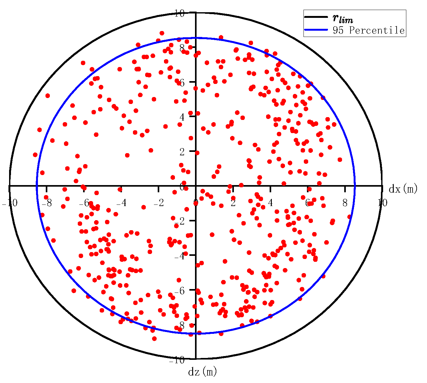
Given the mission profile and operational constraints, the terminal criteria were formally established as follows:

• The height of the vehicle is less than zero;
• The FOV constraints or the overload constraints are violated;
• The vehicle is flying in a direction that is away from the target;
• The vehicle has arrived at the target successfully.

It is of significant importance to note that the current episode will be terminated if the constraints are violated. In such an instance, the agent will not receive a terminal reward. This incentive is sufficient to encourage the agent to learn to satisfy the constraints; therefore, no negative reward is required when the constraint is violated.

4.3. Policy Optimization

In light of the satisfactory performance of GRU in long-term historical memory, a GRU layer was introduced into the actor network and the critic network with the objective of enhancing the generalization ability of the policy under different task conditions. This integration enabled the policy to adapt to varying tasks through the updating of the hidden states of the GRUs.

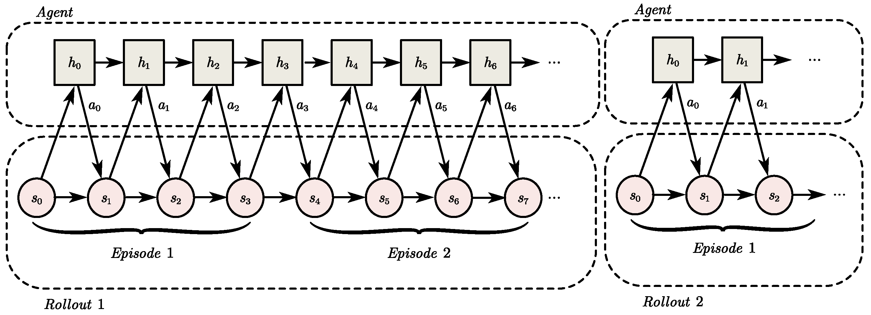
It should be noted that when GRU layers are introduced into policy and value networks, the way to update the hidden state of the GRU layer during the rollout collection process has a significant impact on the training effect. Inspired by [33,37], the hidden state was reset before the start of each rollout. However, the hidden state of each episode in the same rollout was inherited from the previous episode. The interaction protocol between the learning agent and its operational environment is illustrated in Figure 5. It should be noted that the length of each episode may vary, although this is not explicitly shown in Figure 5. Through this design, the aim was to encourage the agent to update the parameters of the GRU layer so that updates to its hidden state could be used to describe an embedded representation of the current environment or task. This provided the agent with multi-level input features for rapid adaptation to different environments and tasks, thereby enhancing the adaptability and generalization performance of the final network.

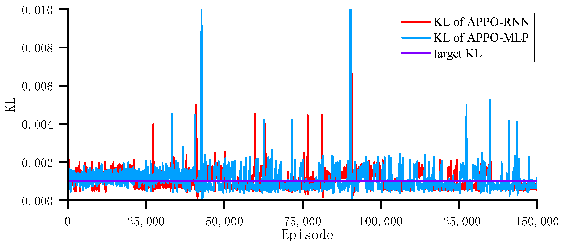
The PPO algorithm has two versions of the objective function. The first is the clipped surrogate objective, whose expression is shown in Equation (2). The second involves incorporating the KL divergence into the objective function as a penalty, and the penalty coefficient is adaptively adjusted so that the KL divergence can reach a specific target value $d_{targ}$ during each policy update.

In general, it is more straightforward to achieve convergence when utilizing the clipped surrogate objective. However, this approach inevitably requires a longer training process. In contrast, it is challenging to achieve convergence when employing the adaptive KL penalty coefficient. Therefore, in order to strike a balance between the speed and stability of the training process, the two aforementioned methods were combined in a novel manner, whereby the clipped factor $ϵ$ and the learning rate ${\alpha }_{\theta }$ of the policy network were adaptively adjusted in order to achieve the target value of the KL divergence $d_{targ}$, that is,

$$ϵ=\left\{\begin{array}{cc}min({ϵ}_{max},1.5ϵ)\hfill & \mathrm{if}d<{\displaystyle \frac{1}{2}}{d}_{targ}\hfill \\ max({ϵ}_{min},1.5ϵ)\hfill & \mathrm{if}d>2d_{targ}\hfill \\ ϵ\hfill & \mathrm{others}\hfill \end{array}\right.$$

(38)

$${\alpha }_{\theta }=\left\{\begin{array}{cc}1.5{\alpha }_{\theta }\hfill & \mathrm{if}d<{\displaystyle \frac{1}{2}}{d}_{targ}\mathrm{and}ϵ>{\displaystyle \frac{1}{2}}{ϵ}_{max}\mathrm{and}{\alpha }_{\theta }<{\alpha }_{\theta }^{max}\hfill \\ {\displaystyle \frac{1}{1.5}}{\alpha }_{\theta }\hfill & \mathrm{if}d>2d_{targ}\mathrm{and}ϵ<2{ϵ}_{min}\mathrm{and}{\alpha }_{\theta }>{\alpha }_{\theta }^{min}\hfill \\ {\alpha }_{\theta }\hfill & \mathrm{others}\hfill \end{array}\right.$$

(39)

In the training phase, the experience data were fully utilized through the conduct of E update epochs, The training process involved a range of generic operations, including ratio calculation, the computation of various losses, and gradient clipping. The adaptive PPO (APPO) algorithm is shown in Algorithm 2.

Algorithm 2 Adaptive PPO (APPO) algorithm

Input: Target value of the KL divergence $d_{targ}$, number of epochs M Output: The optimized parameters of actor $\theta$, and critic w 1: Initialize network parameters, including the actor $\theta$, and critic w 2: for epoch = $1:M$ do 3:     Initialize replay buffer R and reset the hidden states of the RNNs 4:     for episodes = $1:N$ do 5:         Reset the environment; 6:         while not done do 7:            Obtain the current observation $s_t$ 8:            The observation $s_t$ is fed to the actor to obtain the action $a_t$ 9:            Execute one step in the environment 10:           Store $(o_t,a_t,r_t,don{e}_t)$ into R 11:        end while 12:     end for 13:     Calculate discounted returns G and advantages $\widehat{A}$ 14:     for opt = $1:E$ do 15:      Calculate policy network loss, value network loss, and KL divergence 16:        Update $\theta ,w$ 17:        Adjust the clipped factor $ϵ$ and the learning rate ${\alpha }_{\theta }$ 18:     end for 19: end for 20: return The optimized parameters $\theta ,w$

5. Simulation Results

5.1. Training Scenarios

The parameters of the vehicle referenced in [12] were adopted; the full parameters of the vehicles are given in

Table 1. Vehicle parameters.

Parameter	Value	Parameter	Value
Mass m (kg)	1600	Reference area $S_{ref}$ (${\mathrm{m}}^2$)	0.5026
Guidance period (s)	0.5	FOV angle limit (degrees)	60
Angle of attack $\alpha$ (degrees)	$[0,28]$	Bank angle $\sigma$ (degrees)	$[-180,180]$
Angle of attack rate $\Delta \alpha$ (degrees/s)	[−5, 5]	Bank angle rate $\Delta \sigma$ (degrees/s)	[−40, 40]
Observation standard deviation ${ϵ}_{obs}$	0.003	Aerodynamic lift coefficient of variation (%)	[−5, 5]
Aerodynamic drag coefficient of variation (%)	[−5, 5]	Atmospheric density variation (%)	[−5, 5]

, and the detail expressions of the aerodynamic coefficients $C_L$ and $C_D$ can be found in ref. [12].

In order to ensure that the agent exhibits good generalization ability, it was trained on a range of initial conditions. The details of the initial conditions are listed in

Table 2. Initial conditions.

Parameter	Value	Parameter	Value
Range $R_{init}$ (km)	[120, 120]	Altitude $h_{init}$ (km)	[28.8, 29.2]
Velocity $V_{init}$ (m/s)	[2060, 2120]	Flight path angle ${\gamma }_{init}$ (degrees)	[−5, 0]
Azimuth ${\psi }_{init}$ (degrees)	[−10, 10]	Heading error $\delta {\psi }_{init}$ (degrees)	[−8, 8]
Angle of attack ${\alpha }_{init}$ (degrees)	[1, 3]	Bank angle ${\sigma }_{init}$ (degrees)	[−2, 2]
Desired impact time $T_d$ (s)	[75, 80]	Target maximum speed $V_{T_{max}}$ (m/s)	15.0
Target maximum acceleration $a_{T_{max}}$ (${\mathrm{m}/\mathrm{s}}^2$)	0.5

.

It should be noted that four-layer network structures are frequently employed in DRL applications [38]. Accordingly, a four-layer neural network was employed to implement the policy and value functions, where the first hidden layer of the policy and value functions was a GRU [39] layer. The network architectures are shown in

Table 3. Network layer size.

	Policy Network		Value Network
Layer	Size	Activation	Size	Activation
Input layer	(10, 100)	tanh	(10, 100)	tanh
GRU layer	(100, 44)	tanh	(100, 22)	tanh
Hidden layer 2	(44, 20)	tanh	(22, 5)	tanh
Output layer	(20, 2)	linear	(5, 1)	linear

.

5.2. Training Results

Table 4. Hyperparameters in the reward function.

Parameter	Value	Parameter	Value	Parameter	Value	Parameter	Value
${\beta }_{miss}$	0.2	${\beta }_{time}$	0.05	${\beta }_{dive}$	0.01	${\beta }_e$	0.01
$\xi$	10	${\kappa }_{\mathsf{\Omega }}$ (rad/s)	0.1	${\kappa }_t$ (s)	0.5	${\kappa }_{\gamma }$ (rad)	${\delta }_{\gamma }\left(t_0\right)/2$
${\kappa }_{V_M}$ (m/s)	200	${ϵ}_r$ (m)	10	${ϵ}_t$ (s)	0.5	${\gamma }_{dive}$ (degrees)	75

and

Table 5. Hyperparameter settings.

Parameter	Value	Parameter	Value
Maximum episode steps	800	Maximum epochs M	2500
Collected episodes per epoch N	60	Update epochs E	20
Discounting factor,$\gamma$	0.95	Value network learning rate ${\alpha }_w$	$2.0\times {10}^{-3}$
Maximum learning rate ${\alpha }_{\theta }^{max}$	$1.5\times {10}^{-3}$	Minimum learning rate ${\alpha }_{\theta }^{min}$	$1.5\times {10}^{-5}$
Maximum clipped factor ${ϵ}_{max}$	0.5	Minimum clipped factor ${ϵ}_{min}$	0.01
Target KL divergence $d_{targ}$	0.001

provide a detailed list of the hyperparameter values used during the training process. In practice, the selection of appropriate hyperparameters is often a crucial determinant of the performance of APPO. Different problems may require the use of different sets of hyperparameters. Accordingly, these hyperparameters were tuned for the guiding problem based on a series of trial-and-error tests.

For comparison, simulations were also performed that replaced the GRU layer with an MLP layer. For the sake of simplicity, the APPO algorithm with GRU is henceforth referred to as APPO-GRU, and the APPO algorithm employing an MLP layer is referred to as APPO-MLP.

The results of comparing the learning curves are shown in Figure 6. The figure clearly demonstrates that the introduction of the GRU layer resulted in a significant increase in the average steady-state reward value. This also validated the previous analysis in this paper, which indicated that using the hidden state of the GRU layer as a deep embedded representation of environmental features could effectively enhance the adaptability and generalization performance of the agent.

The final impact-time error change process during the training process is illustrated in Figure 7. As can be observed from Figure 7, the arrival-time error of APPO-GRU eventually converged to around 0.2 s, while the arrival-time error of APPO-MLP converged to approximately 0.7 s. This also demonstrated that the incorporation of the GRU layer could effectively enhance the guidance performance of the agent.

The incorporation of a GRU layer contributed to the agent’s performance through two primary mechanisms. Primarily, the hidden state of the GRU layer enabled the agent to delineate the characteristics of various task scenarios, thereby augmenting its capacity for generalization and robustness. Secondly, the hidden state could retain the historical information of the trajectory, endowing the guidance policy with the capability to draw insights from the historical state.

Furthermore, Figure 8 illustrates the curves of the KL divergence of the policy throughout the training process. This figure demonstrates that the proposed adaptive PPO algorithm could maintain the KL divergence of the policy at a level closely aligned with the target KL divergence, thereby ensuring that the training process remained stable and ultimately converged.

5.3. Test Results

To verify the impact-time-control capability of the proposed guidance policy, simulations were performed on scenarios with the same initial state but different preset impact times. The initial state settings are shown in

Table 6. Initial state of vehicles.

Parameter	Value	Parameter	Value
Range (km)	120	Altitude (km)	29
Velocity (m/s)	2100	Flight path angle (degrees)	−2
Azimuth (degrees)	5	Heading error (degrees)	4
Angle of attack (degrees)	1.5	Bank angle (degrees)	0
Desired impact time (s)	76, 78, 80

and the preset impact times were 76, 78, and 80 s, respectively. For comparison, the PNG law was also simulated. The simulation results for different desired arrival times are presented in Figure 9 and Figure 10. In addition, the final miss distance, flight path angle, and arrival-time error results are listed in

Table 7. Final state for different impact times.

Scenarios	Miss Distance (m)	Impact Time (s)	Velocity (m/s)	Impact Angle (deg)
$T_d=76$ s	7.146	76.367	991.347	−79.766
$T_d=78$ s	8.453	77.795	1003.193	−82.438
$T_d=80$ s	9.022	79.674	975.535	−83.945
PNG	2.334	79.853	559.952	−18.650

.

As illustrated in Figure 9, the proposed ITGC law primarily controlled the arrival time by controlling the vehicle to turn in the horizontal plane. In other words, different specified arrival times were achieved by controlling the magnitude of lateral maneuvers; the larger the specified arrival time, the greater the amplitude of the turning maneuvers in the lateral plane. At the same time, it can be observed from Table 7 that the impact time errors of the proposed ITCG law were all less than 0.5 s. Furthermore, Figure 10f illustrates the FOV angle curves for different specified arrival times; it can be seen that the proposed ITGC law was capable of maintaining the FOV constraint at all times, thereby providing further evidence of the efficiency of the proposed ITCG law.

It should be noted that while the PNG law could also meet FOV constraints, it was not capable of controlling impact time or diving attack. Moreover, as can be found in Figure 10b, the terminal velocity of the vehicle guided by the PNG law was around 600 m/s, while the terminal velocities of the proposed guidance law were around 1000 m/s. Therefore, the proposed ITCG law also demonstrated significant superiority over PNG in terms of optimizing performance metrics.

It should be noted that, as shown in Figure 10d, when the ITCG law proposed in this paper was employed, the bank angle frequently alternated between $-\pi$ and $\pi$. However, this did not violate the bank angle rate constraint specified in Equation (31b), as the bank angle adjustments were controlled through the minimum rotation angle (as illustrated in Figure 11).

According to Figure 11, we can define the corresponding vectors for $\sigma$ and ${\sigma }_c$ as follows:

$$\begin{array}{c}\hfill \mathit{q}={\left[cos\sigma ,sin\sigma ,0\right]}^T\end{array}$$

(40a)

$$\begin{array}{c}\hfill {\mathit{q}}_c={\left[cos{\sigma }_c,sin{\sigma }_c,0\right]}^T\end{array}$$

(40b)

Subsequently, the cross-product of $\mathit{q}$ and ${\mathit{q}}_c$ can be calculated using the following equation:

$$\mathit{q}\times {\mathit{q}}_c={\left[0,0,sin{\sigma }_{c}cos\sigma -cos{\sigma }_{c}sin\sigma \right]}^T={\left[0,0,sin\left({\sigma }_c-\sigma \right)\right]}^T$$

(41)

Therefore, according to Figure 11, when $sin\left({\sigma }_c-\sigma \right)<0$, the bank angle $\sigma$ rotates clockwise towards the commanded bank angle ${\sigma }_c$, whereas when $sin\left({\sigma }_c-\sigma \right)>0$, $\sigma$ rotates counterclockwise towards ${\sigma }_c$.

Finally, Equation (31b) can be rewritten as follows:

$$\Delta {\sigma }_c=\left\{\begin{array}{cc}\mathrm{clip}\left({\displaystyle \frac{{\sigma }_c-\sigma +2\pi }{\Delta t}},-\Delta {\sigma }_{max},\Delta {\sigma }_{max}\right),\hfill & \mathrm{if}sin\left({\sigma }_c-\sigma \right)<0\hfill \\ \mathrm{clip}\left({\displaystyle \frac{\sigma -{\sigma }_c-2\pi }{\Delta t}},-\Delta {\sigma }_{max},\Delta {\sigma }_{max}\right),\hfill & \mathrm{if}sin\left({\sigma }_c-\sigma \right)>0\hfill \end{array}\right.$$

(42)

Taking the flight trajectory with $T_d=76\mathrm{s}$ as an example, in Figure 10d, the bank angle of the UAV changed from $-177.28\mathrm{deg}$ to $177.76\mathrm{deg}$ at $t=5\mathrm{s}$. However, the actual change in the bank angle was only $-4.96\mathrm{deg}$ During the guidance cycle, the corresponding bank angle rate of change was $-4.96\mathrm{deg}/\mathrm{s}$, which was significantly lower than the bank angle rate constraint specified in Table 1.

5.4. Monte Carlo Simulations

Monte Carlo simulations are performed to assess the adaptability and robustness of the proposed ITCG law, considering factors such as aerodynamic disturbances and measurement noise. The initial state variables of the vehicle were stochastically generated based on the parameter ranges outlined in Table 2, while the environmental uncertainties are defined in Table 1. The results of 500 independent Monte Carlo trials are summarized in Figure 12, Figure 13 and Figure 14.

As illustrated in Figure 12b, the terminal velocity of the vehicle was approximately 1000 m/s, its velocity loss was significantly less than that of the PNG law. The results presented in Figure 12c shows that the final flight path angles were all around $-{80}^{\circ }$, ensuring compliance with the dive-attack specifications. Furthermore, Figure 12d illustrates that the FOV constraints were also satisfied. The results indicate that the proposed guidance law exhibited exceptional robustness, even when subjected to aerodynamic deviations and sensor noise.

To gain further insight into guidance performance, a series of key variables were subjected to statistical analysis, the results of which are presented in

Table 8. The statistical results of the Monte Carlo experiment.

Parameters	Mean	Min	Max
Impact angle (degrees)	−83.137	−89.999	−75.357
Impact-time error (s)	−0.0601	−0.4986	0.4990
Miss distance (m)	6.2235	0.4892	9.4947
Impact velocity	1003.53	880.43	1082.00

. Figure 13 illustrates the distribution of the miss distance in the 2D plane, and Figure 14 presents the statistical histograms that include the miss distance, impact time error, terminal flight path angle, and terminal velocity.

Figure 13 depicts the impact point distribution results from Monte Carlo simulations. As illustrated in Figure 13, despite the presence of aerodynamic parameter deviations and observation noise, the miss distances of the proposed guidance policy remained within 10 m, with impact time errors below 0.5 s. The results demonstrate that the proposed ITCG law displayed robust performance. Furthermore, Table 8 indicates that the minimum impact velocity was 880.43 m/s, which was considerably higher than the impact velocity of the PNG law.

6. Conclusions

This study proposed a DRL-based ITCG law for a high-speed UAV with time-varying velocity, enabling impact-time control and dive attack while maintaining FOV constraints. Firstly, a reinforcement learning framework was designed for high-speed UAV guidance with time-varying velocity, in which the guidance system mapped observations, including time-to-go estimation, to the commanded acceleration of the vehicle. Secondly, a multi-objective reward architecture was developed to jointly optimize both time-constrained impact and dive attack. Furthermore, in order to improve the adaptability of the guidance law, environmental uncertainties were considered during the training process. In particular, GRU layers were introduced into the policy network and value network to make the policy adaptive to different task scenarios. Finally, simulations were conducted in various challenging scenarios, and the results illustrated that the proposed ITCG law exhibited good performance even in the presence of aerodynamic parameter deviation and environmental uncertainties.

Future research will prioritize three key directions. First, the development of an integrated guidance framework incorporating simultaneous impact-time and terminal-angle control is expected to significantly enhance high-speed UAVs’ operational capabilities in executing complex mission profiles; second, it would be beneficial to consider extending this method to integrated guidance-and-control frame; third, based on the establishment of communication links among UAV swarms, multi-agent reinforcement learning (MARL) techniques could be utilized to construct a distributed cooperative guidance decision-making method, enabling the realization of collective intelligence in a true sense.