A Coverage-Based Cooperative Detection Method for CDUAV: Insights from Prediction Error Pipeline Modeling

Abstract

To address the challenges of detection and acquisition caused by trajectory prediction errors during the midcourse–terminal guidance handover phase in cross-domain unmanned aerial vehicles (CDUAV), this study proposes a collaborative multi-interceptor detection coverage optimization method based on predictive error pipeline modeling. Firstly, we employ nonlinear least squares to fit parameters for the motion model of CDUAV. By integrating error propagation theory, we derive a recursive expression for error pipelines under t-distribution and establish a parametric model for the target’s high-probability region (HPR). Next, we analyze target acquisition scenarios during guidance handover and reformulate the collaborative detection problem as a field-of-view (FOV) coverage optimization task on a two-dimensional detection plane. This framework incorporates the target HPR and the seeker detection FOV models, with an objective function defined for coverage optimization. Finally, inspired by wireless sensor network (WSN) coverage strategies, we implement the starfish optimization algorithm (SFOA) to enhance computational efficiency. Simulation results demonstrate that compared to Monte Carlo statistical methods, our parametric modeling approach reduces prediction error computation time from 15.82 s to 0.09 s while generating error pipeline envelopes with 99% confidence intervals, showing superior generalization capability. The proposed collaborative detection framework effectively resolves geometric coverage optimization challenges arising from mismatches between target HPR and FOV morphology, exhibiting rapid convergence and high computational efficiency.

1. Introduction

Cross-domain unmanned aerial vehicles (CDUAV), with fast flight speed and strong maneuverability, glide at high speed in a multilayer atmospheric physical domain, and their target trajectories are difficult to accurately predict, so the defender can only predict the target’s high probability region (HPR) in the future according to the tracking information [1,2,3]. Thus, the vehicle can effectively break through the existing air defense system and become a significant air and space threat. In recent years, although there have been many studies on cooperative capture, most of them have focused on the terminal guidance phase, and few of them have dealt with cooperative capture in the midcourse–terminal guidance handover shifts. If the problem cannot be effectively solved, it will be difficult to close the killing chain. At the same time, due to the detection performance of a single interceptor’s seeker being limited by the role of distance and field-of-view (FOV) angle constraints [4,5,6], it is difficult to achieve the effective detection and capture of a wide range of target HPR; there is a “detection blind zone” and “capture lag” and other issues. The success rate of midcourse–terminal guidance handover is seriously affected. Therefore, studying the detection and capture of midcourse–terminal guidance handover targets in CDUAV is significant.

From the perspective of target trajectory prediction, there are two primary methods: one is based on the statistical analysis of the data set to carry out the prediction [7,8,9]. This type of method has excellent performance in short-term prediction. Still, it is limited because it has not been introduced into the vehicle dynamics characteristics, and it is not easy to adapt to the accuracy needs of medium- and long-term prediction. The second is trajectory prediction based on the vehicle dynamics model, and the typical methods include filter extrapolation [10], position fitting [11,12], parameter fitting [13,14], and deep learning [15,16,17]. Among them, the filter extrapolation and position fitting algorithms can only maintain the prediction accuracy within a limited time window, and the deep learning algorithm can predict the parameter time series with a high degree of nonlinearity. Still, it requires many high-quality trajectory datasets, and it is not easy to guarantee the algorithm’s generalization. In trajectory prediction, CDUAV is a noncooperative target; in the case of insufficient a priori information, the prediction model differs from the real model and leads to the transmission and accumulation of error with the extension of time. The target HPR will gradually increase with the space error, showing diffusion and time-varying characteristics. Therefore, the study of the prediction error pipeline is of great significance for determining the spatial range of the target under the predicted moment and formulating the detection and capture strategy of the interceptor. Sun et al. [12] used Monte Carlo simulation to study the morphology and two-dimensional cross-section of the error pipeline; based on this, Hu et al. [18] proposed a trajectory prediction method based on the regression of the Gaussian process and analyzed and investigated the trajectory error envelope under the 95% confidence interval. For the characteristics, Li et al. [19] analyzed the influence of each element on the characteristics of the error pipeline from four aspects, such as end-point error correction, parameter error correction, prediction error, and pneumatic error, combined with Monte Carlo simulation. However, there are relatively few researchers in this field, and the existing methods mainly rely on Monte Carlo simulation techniques based on statistical analysis and Gaussian process regression models, which require high-quality data sets and suffer from low computational processing efficiency, making it difficult to deal with the time-varying characteristics of the target HPR effectively.

From the point of view of interceptor detection and capture, according to the number of interceptors, it can be categorized into single-body or cooperative detection and capture. Single-body capture mainly applies to continuous and stable target tracking, high measurement accuracy, and short data delay, in which the target motion trajectory prediction error is small, and the target HPR is wholly located within the FOV of the seeker [20]. However, for noncooperative targets such as CDUAV, under the combined effect of significant tracking data error and inaccurate fitting of motion model parameters, the target HPR increases rapidly. When it exceeds the constraints of the FOV of a single interceptor, it will produce a detection blind zone, leading to capture delay and affecting the handover success rate. Therefore, a coordinated detection approach is now commonly adopted [21,22]. Through the numerical advantage to make up for the lack of detection capability of individual interceptors, a space-for-time strategy is adopted to utilize multi-field-of-view coordinated coverage technology to achieve the timely detection and capture of targets within the limited handover window. The commonly used methods for the coverage optimization problem include the area segmentation method based on the Voronoi diagram [23,24,25], the geometric analysis method, and the coverage optimization method based on WSN. Among them, the Voronoi diagram-based area coverage optimization method performs well when dealing with static fixed areas. Still, for the case where the boundary area is uncertain and dynamically changing, the frequent updating of the Voronoi diagram will lead to high computational cost and delay, and there are obvious limitations. Although the geometric analysis method is accurate and fast, it usually needs to simplify the target HPR morphology, and the generalization is poor. Zhou et al. [26] define the target HPR as a rectangular region in the 2D plane and the FOV of the seeker as a square region and then use the geometric analysis method to study the coverage relationship under similar morphology; Luo et al. [27] define the target HPR as a spherical region in 3D space, and the FOV as a spherical-topped conical state.. Based on the geometric size-matching relationship between the two, a geometric modeling method is used to solve the coverage problem of multiple dome cones on the sphere. This geometric analytic method is based on quantifying the relative spatial sizes of the target HPR and the FOV, dividing the coverage relationship between the two into several characteristic intervals, and modeling the geometric computation by constructing segmented discriminative conditions. The method has analytical advantages under geometric form matching conditions (e.g., regular symmetric configurations such as circle–circle, rectangle–rectangle, etc.). Still, when dealing with heterogeneous combinations (e.g., circle–ellipse) or nonregular geometries, geometric analytic methods are difficult to solve, leading to limitations in the generalization ability of the method. In contrast, the development of the WSN-based coverage optimization method is more mature [28,29,30]. Zhu et al. [31] commence their study by addressing two fundamental issues in the field: coverage and connectivity. The primary focus of the study is on the classification of coverage problems, and the identification of coverage methods, objective functions, and related algorithms. The subsequent step involves the construction of a framework for addressing WSN coverage optimization problems. Deif et al. [32] conducted a study on the subject of planned deployment algorithms for WSN coverage optimization problems. The study involved an analysis of the advantages and disadvantages of a range of algorithms, including evolutionary algorithms, swarm intelligence algorithms, geometric analytic methods, and artificial potential fields. Anusuya et al. [33] propose a multi-objective extension to the traditional single-objective WSN coverage optimization problem. The latter seeks to maximize coverage, while the former encompasses both coverage and energy loss, thus enriching the WSN coverage optimization scheme. Its optimization idea is: in a limited area, through the use of swarm intelligence algorithm to optimize the arrangement of nodes, based on the network connection, by seeking the global optimal solution, to achieve high coverage with fewer nodes, to satisfy the network coverage optimization needs. Compared with the geometric resolution method, it can solve the geometric coverage problem between the morphology mismatch regions under the two-dimensional plane. In addition, the terminal guidance cooperative coverage fencing design method also has essential reference value for the coverage optimization research [34,35,36]; although there are some differences in the two coverage mechanisms, the form of coverage has a similarity and has the conditions for technology migration.

In summary, in order to solve the problem of detection and capture of CDUAV under the influence of trajectory prediction error, this paper proposes a multi-interceptor cooperative detection coverage optimization method based on prediction error pipeline modeling. Firstly, the parameters of the target motion model are fitted by the nonlinear least squares method, and the recursive expression of the trajectory prediction error pipeline is derived to construct the parameterized model of the target HPR; secondly, according to the conditions of the midcourse–terminal guidance handover window, the interceptor’s detection and capture posture of the target is analyzed, and the collaborative detection and capture problem is transformed into the optimization of HPR coverage by the FOV on the two-dimensional detection cross-section, and, accordingly, the target HPR model and the seeker detection FOV model, and the FOV coverage function is constructed as the objective function of coverage optimization; finally, the Starfish intelligent optimization algorithm is used to solve the coverage optimization problem with the objective of maximum coverage. The implementation path of the approach proposed in this paper is a “prediction-transformation-coverage” process framework, and the technical scheme is “error parametric modeling-geometric-mathematical problem transformation in the 2D plane-WSN coverage optimization solution”, and the main application scenarios are the midcourse–terminal guidance. The main application scenario is the cooperative detection of the target HPR by multi-interceptor seekers during the midcourse–terminal guidance handover phase, and the corresponding constraints include the target motion model parameters, tracking system parameters, detection system parameters, optimization algorithm parameters, etc. The key contributions of this work are as follows:

(1)

The nonlinear least squares method is used to fit the parameters of the target motion model, and the recursive expression of the error pipeline for trajectory prediction under the t-distribution is derived according to the theory of error propagation to construct a parameterized model of the target HPR. In terms of error prediction, compared with statistical methods such as Monte Carlo simulation, the error pipeline envelope has faster convergence speed and stronger generalization.

(2)

A cooperative detection coverage optimization solution framework is proposed to analyze the multi-interceptor cooperative detection capture posture in conjunction with handover window. The problem is transformed into a two-dimensional detection cross-section of the FOV coverage optimization problem for HPR, which leads to the construction of an ellipsoidal model for HPR under a small-sample distribution with stronger generalizability and a seeker detection FOV model. The FOV coverage objective function and the corresponding boundary constraints are established to form closed-loop problem-solving.

(3)

Drawing on the WSN coverage optimization scheme, the geometric coverage optimization problem of mismatch between the target HPR and the FOV pattern is solved, and the Starfish intelligent optimization algorithm is adopted to accelerate the solution efficiency and further expand the solution ideas of the cooperative detection coverage optimization problem.

2. Prediction Error Pipeline Modeling

Trajectory prediction for CDUAV is essentially an estimation of its state or control law, and subtle changes in its control parameters can lead to a wide range of position changes. Therefore, carrying out predictions only by extrapolating filters or fitting position information cannot satisfy the medium- to long-term, high-precision prediction needs of the defense for CDUAV trajectories. A standard method is to select reasonable motion model parameters for estimation to improve the prediction accuracy and duration. This paper uses the simplified set of three-degrees-of-freedom kinematic equations of CDUAV as the kinematic model for trajectory extrapolation. The rates of change in velocity, inclination, and declination are selected as the maneuvering parameters, which are combined with the kinematic model to achieve high-precision, medium- and long-term trajectory prediction by predicting the maneuvering parameters. However, due to the maneuverability of the CDUAV, there is bound to be a difference between the fitted parameter model and the real motion law, and the prediction error increases gradually with the increase in prediction time. Therefore, the focus is on modeling the error generated during parameter prediction and the trajectory prediction error pipeline to provide theoretical and data support for mid–end guided handover target detection and capture based on predicted hit points.

This paper proposes a pipeline modeling method for target prediction error, which focuses on solving the problem of the coupling analysis of multiple error sources and their transfer mechanisms, and adopts a pipeline boundary generation method based on the 0.99 confidence interval. Specifically, the method focuses on the following three aspects: (1) quantitative analysis of the inherent error of the system; (2) accurate modeling of the error transfer path; and (3) probabilistic boundary construction of the confidence interval. Although environmental disturbances (e.g., atmospheric perturbations) introduce additional error components, their effects are relatively limited. Therefore, to simplify the model complexity and highlight the feasibility and validation of the parametric modeling approach, the influence of such disturbance terms is not separately considered in the modeling process in this study.

2.1. CDUAV Motion Model

The CDUAV kinematic model is used to construct the vehicle dynamics equations oriented to trajectory prediction. Without considering the Earth’s rotation, the model’s three-degrees-of-freedom dynamics equations in the half-velocity (Velocity–Turn–Climb, VTC) coordinate system can be expressed as follows [37]:

$$\{\begin{array}{l}{\displaystyle \frac{dr}{dt}}=v\sin \theta \\ {\displaystyle \frac{d\varphi }{dt}}={\displaystyle \frac{v\cos \theta \sin \psi }{r\cos \phi }}\\ {\displaystyle \frac{d\phi }{dt}}={\displaystyle \frac{v\cos \theta \cos \psi }{r}}\\ {\displaystyle \frac{dv}{dt}}=-{\displaystyle \frac{D}{m}}-g\sin \theta \\ {\displaystyle \frac{d\theta }{dt}}={\displaystyle \frac{L\cos \sigma }{mv}}+{\displaystyle \frac{\cos \theta }{v}}({\displaystyle \frac{v^2}{r}}-g)\\ {\displaystyle \frac{d\psi }{dt}}={\displaystyle \frac{L\sin \sigma }{mv\cos \theta }}+{\displaystyle \frac{v\cos \theta \sin \psi \tan \phi }{r}}\end{array}$$

(1)

The meanings of the parameters in the model are shown in

Table 1. Meaning of each parameter in the model.

Parameter	Meaning	Parameter	Meaning
$r$	geocentric distance	$\theta$	flight path angle
$\varphi$	Latitude	$\psi$	heading angle
$\phi$	longitude	$\sigma$	bank angle
$v$	velocity	$L$	aerodynamic lift
$m$	mass	$D$	aerodynamic drag

.

And the aerodynamic model is as follows:

$$\{\begin{array}{l}L={\displaystyle \frac{\rho v^2}{2}}{C}_L\left(\alpha \right)S\\ D={\displaystyle \frac{\rho v^2}{2}}{C}_D\left(\alpha \right)S\end{array}$$

(2)

where $C_L$ and $C_D$ denote the vehicle’s lift and drag coefficients, $\alpha$ represents the angle of attack, $S$ indicates the reference area, and $\rho$ signifies the atmospheric density at the corresponding flight altitude.

The components $L\cos \sigma$ and $L\sin \sigma$ of the aerodynamic lift and the aerodynamic drag $D$ directly determine the states of motion of the vehicle; the aerodynamic acceleration is obtained from Newton’s second law.

$$\mathrm{a}=\left[\begin{array}{l}{a}_v\\ a_t\\ a_c\end{array}\right]={\displaystyle \frac{1}{m}}\left[\begin{array}{c}D\\ L\sin \sigma \\ L\cos \sigma \end{array}\right]={\displaystyle \frac{\rho v^2}{2}}\left[\begin{array}{c}{\displaystyle \frac{C_D\left(\alpha \right)S}{m}}\\ {\displaystyle \frac{C_L\left(\alpha \right)S\sin \sigma }{m}}\\ {\displaystyle \frac{C_L\left(\alpha \right)S\cos \sigma }{m}}\end{array}\right]$$

(3)

The aerodynamic acceleration is directly related to the atmospheric density $\rho$. In order to avoid the strong nonlinearity caused by the alteration of the vehicle’s gliding altitude, based on the dynamic pressure expression $q=0.5\rho v^2$, a set of variably stabilized aerodynamic parameters can be obtained from Equation (3).

$$\mathrm{u}=\left[\begin{array}{l}{\alpha }_v\\ {\alpha }_t\\ {\alpha }_c\end{array}\right]=\left[\begin{array}{c}{\displaystyle \frac{C_D\left(\alpha \right)S}{m}}\\ {\displaystyle \frac{C_L\left(\alpha \right)S\sin \sigma }{m}}\\ {\displaystyle \frac{C_L\left(\alpha \right)S\cos \sigma }{m}}\end{array}\right]$$

(4)

where ${\alpha }_v$ denotes the drag parameter in the velocity vector’s opposite direction, ${\alpha }_t$ represents the lateral turning force parameter in the horizontal plane, and ${\alpha }_c$ indicates the longitudinal climbing force parameter in the skyward plane.

The CDUAV can achieve different maneuver modes by adjusting the angle of attack $\alpha$ and bank angle $\sigma$. For the defender, the stressed area $S$, mass $m$, and angle of attack $\alpha$ are generally unknown or difficult to measure. Therefore, constructing the CDUAV motion model requires the integrated estimation of aerodynamic parameters $\mathrm{u}$. To improve motion model parameter matching accuracy, the lift parameter ${\alpha }_l$ is defined as follows:

$${\alpha }_l=\sqrt{{\alpha }_t^2+{\alpha }_c^2}={\displaystyle \frac{C_L\left(\alpha \right)S}{m}}$$

(5)

Thus, the motion model of the CDUAV can be transformed into the following:

$$\{\begin{array}{l}{\displaystyle \frac{dr}{dt}}=v\sin \theta \\ {\displaystyle \frac{df}{dt}}={\displaystyle \frac{v\cos \theta \sin \psi }{r\cos \phi }}\\ {\displaystyle \frac{d\phi }{dt}}={\displaystyle \frac{v\cos \theta \cos \psi }{r}}\\ {\displaystyle \frac{dv}{dt}}=-{\displaystyle \frac{{\alpha }_v\rho v^2}{2}}-g\sin \theta \\ {\displaystyle \frac{d\theta }{dt}}={\displaystyle \frac{{\alpha }_l\rho v\cos \sigma }{2}}+{\displaystyle \frac{\cos \theta }{v}}\left({\displaystyle \frac{v^2}{r}}-g\right)\\ {\displaystyle \frac{d\psi }{dt}}={\displaystyle \frac{{\alpha }_l\rho v\sin \sigma }{2\cos \theta }}+{\displaystyle \frac{v\cos \theta \sin \psi \tan \phi }{r}}\end{array}$$

(6)

2.2. CDUAV Trajectory Prediction Error Propagation Model

CDUAV trajectory prediction typically comprises three components: tracking filtering via detection devices, parameter fitting based on nonlinear least squares methods, and integration-based extrapolation using motion models. Correspondingly, trajectory prediction errors originate from filtering, parameter estimation, and integration errors. According to error propagation theory, input errors propagate through the Jacobian matrix of the system state equation in the form of covariance matrices. For a nonlinear function $\mathit{y}=f(\mathit{x})$, given the input variable $\mathit{x}$ and covariance matrix ${\mathit{\Sigma }}_{\mathit{x}}$ and the Jacobian matrix $\mathit{J}$ of the first-order partial derivatives, the output covariance matrix ${\mathit{\Sigma }}_{\mathit{y}}$ is expressed as follows:

$${\mathit{\Sigma }}_{\mathit{y}}=\mathit{J}{\mathit{\Sigma }}_{\mathit{x}}{\mathit{J}}^T$$

(7)

This is different from Monte Carlo simulation, which randomly generates inputs to directly statistically output the covariance matrix. The error covariance matrix obtained from the parametric modeling approach is more efficient and accurate, shorter and less time-consuming, and better able to adapt to the time-varying characteristics of the target HPR.

The three error function relationships and transfers are derived below.

2.2.1. Filter Error Propagation Model

Filtering errors primarily arise from measurement noise in detection systems, model mismatch in target motion, and process noise. Their covariance matrices can be obtained using Kalman filtering algorithms and their variants. During the tracking phase, the target state vector is estimated using the Current Statistical (CS) model and the Unscented Kalman Filter (UKF) algorithm. The underlying principles of the measurement model, CS model, and UKF are not detailed here.

First, the target state vector containing aerodynamic acceleration is established as follows:

$${\mathit{x}}_{k_{ENU}}={[x_k,y_k,z_k,{\dot{x}}_k,{\dot{y}}_k,{\dot{z}}_k,a_{v,k},a_{t,k},a_{c,k}]}^{\mathrm{T}}$$

(8)

where $x_k,y_k,z_k$ denotes the position vector in the East–North–Up (ENU) coordinate system, ${\dot{x}}_k,{\dot{y}}_k,{\dot{z}}_k$ represents the velocity vector in ENU coordinates, $a_{v,k},a_{t,k},a_{c,k}$ is the aerodynamic acceleration vector in the VTC system, and $k$ indicates the tracking time.

Since CDUAV trajectory prediction models typically operate in the VTC system, whereas filtering algorithms provide covariance matrices in the ENU system, the covariance matrix of the target state vector at tracking termination cannot directly characterize filtering errors. It requires a coordinate transformation from ENU to VTC, followed by derivation of the covariance matrix for the terminal target state vector in VTC coordinates using error propagation theory.

The discrete state variable transformation formula from ENU to VTC coordinates is given below:

$$\{\begin{array}{l}{r}_k=z_k+R_e\\ {\varphi }_k=x_k/R_e\\ {\phi }_k=y_k/R_e\\ v_k=\sqrt{{\dot{x}}_k^2+{\dot{y}}_k^2+{\dot{z}}_k^2}\\ {\theta }_k=\arcsin \left(v_{z,k}/v_k\right)\\ {\psi }_k=\arctan \left({v_{x,k}/v}_{y,k}\right)\end{array}$$

(9)

where $R_e$ is the Earth’s radius, and $v_{x,k},v_{y,k},v_{z,k}$ denotes the components along three axes of ENU coordinate system.

For the discrete unknown variables ${\alpha }_{v,k},{\alpha }_{l,k},{\sigma }_k$, combined with Equations (3)–(5), the following is derived from the state vector $a_{v,k},a_{t,k},a_{c,k}$.

$$\{\begin{array}{l}{\alpha }_{v,k}=2a_{v,k}/\rho v^2\hfill \\ {\alpha }_{l,k}=2\sqrt{a_{t,k}^2+a_{c,k}^2}/\rho v^2\hfill \\ {\sigma }_k=\arcsin (a_{t,k}/\sqrt{a_{t,k}^2+a_{c,k}^2})\hfill \end{array}$$

(10)

Then, the target state vector in the VTC coordinate system is as follows:

$$x_k={[r_k,{\varphi }_k,{\phi }_k,v_k,{\theta }_k,{\psi }_k,a_{v,k},a_{l,k},{\sigma }_k]}^{\mathrm{T}}$$

(11)

Next, the target state vector covariance matrix in the ENU coordinate system of the tracking segment is defined as ${\Sigma }_{x_{k_{ENU}}}$ with the following expression:

$${\Sigma }_{x_{k_{ENU}}}=\left[\begin{array}{ccccc}{\sigma }_{x_k}^2& {\sigma }_{x_k}{\sigma }_{y_k}& \cdots & \cdots & {\sigma }_{x_k}{\sigma }_{a_{c,k}}\\ {\sigma }_{x_k}{\sigma }_{y_k}& {\sigma }_{x_y}^2& & & ⋮\\ ⋮& & \ddots & & ⋮\\ ⋮& & & {\sigma }_{a_{t,k}}^2& {\sigma }_{a_{t,k}}{\sigma }_{a_{c,k}}\\ {\sigma }_{x_k}{\sigma }_{a_{c,k}}& \cdots & \cdots & {\sigma }_{a_{t,k}}{\sigma }_{a_{c,k}}& {\sigma }_{a_{c,k}}^2\end{array}\right]$$

(12)

According to the error propagation equations, the target state vector covariance matrix ${\Sigma }_{x_{k_{ENU}}}$ is transformed to the VTC coordinate system:

$${\Sigma }_{x_k}=J_{ENU}^{VTC}{\Sigma }_{x_{k_{ENU}}}{\left(J_{ENU}^{VTC}\right)}^T$$

(13)

where $J_{ENU}^{VTC}$ is the Jacobian matrix of the coordinate transformation equations from ENU to VTC for the target state vector.

2.2.2. Parametric Error Propagation Model

The CDUAV presents complex maneuvering characteristics during cross-domain flight, and state quantities such as its position parameters and its rate of change usually show significant nonlinear fluctuation characteristics, which makes it difficult to realize high-precision modeling and high overfitting risk by traditional fitting methods. In this paper, the nonlinear least squares method is employed for parameter fitting with the relatively stable state variable $\tilde{\dot{v}},\tilde{\dot{\theta }},\tilde{\dot{\psi }}$ in the target motion model. The fitted parameters are defined as the maneuvering parameters, and the differential fitting vector of the target state containing the maneuvering parameters is noted as follows:

$${\tilde{\dot{x}}}_k=[{\tilde{\dot{r}}}_k,{\tilde{\dot{\varphi }}}_k,{\tilde{\dot{\phi }}}_k,{\tilde{\dot{v}}}_k,{\tilde{\dot{\theta }}}_k,{\tilde{\dot{\psi }}}_k{]}^{\mathrm{T}}$$

(14)

Since there is a certain error in the maneuvering parameters estimated by the nonlinear least squares and filtering methods, this error accumulates gradually with the prediction time. Therefore, the residuals ${\mathit{e}}_{nls}$ and variance ${\mathit{\sigma }}_{nls}^2$ of the fitted maneuvering parameters for the tracking segment are calculated with the following expressions:

$$e_{nls}=\left[\begin{array}{l}\dot{v}-\tilde{\dot{v}}\\ \dot{\theta }-\tilde{\dot{\theta }}\\ \dot{\psi }-\tilde{\dot{\psi }}\end{array}\right]$$

(15)

$${\sigma }_{nls}^2=e_{nls}^2/\left(N_1-n\right)$$

(16)

where $N_1$ is the tracking duration; ${\mathit{\sigma }}_{nls}^2$ denotes the residual variance ${\mathit{e}}_{nls}$; for degrees-of-freedom correction and unbiased estimation, the denominator of ${\mathit{\sigma }}_{nls}^2$ is $N_1-n$, and $n$ is the degree of freedom of the fitted function.

According to the variation in the maneuvering parameters in the tracking segment, the benchmark functions of the primary and trigonometric combinations are selected to fit $\tilde{\dot{v}},\tilde{\dot{\theta }},\tilde{\dot{\psi }}$ separately:

$$f\left(a,k\right)=a\left(1\right)\sin \left(a\left(2\right)k+a\left(3\right)\right)+a\left(4\right)k+a\left(5\right)$$

(17)

where $a(1)~a(5)$ are the parameters to be fitted.

The Jacobian matrix is calculated from Equation (17):

$$J={\left[J_1,J_2\cdots ,J_k,\cdots ,J_{N_1}\right]}^T$$

(18)

$$J_k={\left[\begin{array}{c}\sin \left(a\left(2\right)k+a\left(3\right)\right)\\ a\left(1\right)k\cos \left(a\left(2\right)k+a\left(3\right)\right)\\ a\left(1\right)\cos \left(a\left(2\right)k+a\left(3\right)\right)\\ k\\ 1\end{array}\right]}^T$$

(19)

Using the residual variance ${\mathit{\sigma }}_{nls}^2$ from Equation (16), the covariance matrix ${\Sigma }_{\Gamma }$ is established. Through error propagation theory, the covariance matrix ${\mathbf{\Sigma }}_a$ of the predicted maneuvering parameters is back-calculated:

$${\Sigma }_{\Gamma }=J{\Sigma }_a{J}^T=\left[\begin{array}{ccc}{\sigma }_{{\tilde{\dot{v}}}_{k+i}}^2& {\sigma }_{{\tilde{\dot{v}}}_{k+i}}{\sigma }_{{\tilde{\dot{\theta }}}_{k+i}}& {\sigma }_{{\tilde{\dot{v}}}_{k+i}}{\sigma }_{{\tilde{\dot{\psi }}}_{k+i}}\\ {\sigma }_{{\tilde{\dot{v}}}_{k+i}}{\sigma }_{{\tilde{\dot{\theta }}}_{k+i}}& {\sigma }_{{\tilde{\dot{\theta }}}_{k+i}}^2& {\sigma }_{{\tilde{\dot{\theta }}}_{k+i}}{\sigma }_{{\tilde{\dot{\psi }}}_{k+i}}\\ {\sigma }_{{\tilde{\dot{v}}}_{k+i}}{\sigma }_{{\tilde{\dot{\psi }}}_{k+i}}& {\sigma }_{{\tilde{\dot{\theta }}}_{k+i}}{\sigma }_{{\tilde{\dot{\psi }}}_{k+i}}& {\sigma }_{{\tilde{\dot{\psi }}}_{k+i}}^2\end{array}\right]$$

(20)

where ${\Sigma }_a$ is the covariance matrix of the tracking-phase fitted parameters, ${\Sigma }_{\Gamma }$ is the covariance matrix of the prediction-phase parameters via error propagation, $N_2$ is the prediction time instant, and $i=1,2\cdots N_2$, where $i$ is the prediction duration.

Next, following error propagation theory, the covariance matrix ${\Sigma }_{{\tilde{\dot{r}}}_{k+i}},{\Sigma }_{{\tilde{\dot{\varphi }}}_{k+i}},{\Sigma }_{{\tilde{\dot{\phi }}}_{k+i}}$ for the differential $\tilde{\dot{r}},\tilde{\dot{\varphi }},\tilde{\dot{\phi }}$ of the position variables in the target motion model is derived. The expression is provided below:

$${\Sigma }_{{\tilde{\dot{r}}}_{k+i}}=J_{{\tilde{\dot{r}}}_{k+i}}{\mathsf{\Sigma }}_{1_{k+i}}{J}_{{\tilde{\dot{r}}}_{k+i}}^T$$

(21)

$${\Sigma }_{{\tilde{\dot{\varphi }}}_{k+i}}=J_{{\tilde{\dot{\varphi }}}_{k+i}}{\mathsf{\Sigma }}_{2_{k+i}}{J}_{{\tilde{\dot{\varphi }}}_{k+i}}^T$$

(22)

$${\Sigma }_{{\tilde{\dot{\phi }}}_{k+i}}=J_{{\tilde{\dot{\phi }}}_{k+i}}{\mathsf{\Sigma }}_{3_{k+i}}{J}_{{\tilde{\dot{\phi }}}_{k+i}}^T$$

(23)

where ${\mathsf{\Sigma }}_{1_{k+i}},{\mathsf{\Sigma }}_{2_{k+i}},{\mathsf{\Sigma }}_{3_{k+i}}$ is the covariance matrix of the input terms in the position differential equations (the first three terms of Equation (6)), and $J_{{\tilde{\dot{r}}}_{k+i}},J_{{\tilde{\dot{\varphi }}}_{k+i}},J_{{\tilde{\dot{\phi }}}_{k+i}}$ is the Jacobian matrix of the corresponding differential equations.

2.2.3. Integrated Error Propagation Model

The target prediction error based on the CDUAV motion model is propagated by integrating the trajectory of the target motion differential equations. This development is built on the derived filter and parameter error propagation models. The filtering and parameter errors are input uncertainties in constructing the covariance matrix. The matrix is then propagated to the predicted error covariance matrix using the Jacobian matrix of the motion model, thus completing the overall error propagation framework.

First, according to the target motion model, the tracking-phase target state vector based on the fitted maneuvering parameters is obtained as follows:

$${\tilde{x}}_k=[{\tilde{r}}_k,{\tilde{\varphi }}_k,{\tilde{\phi }}_k,{\tilde{v}}_k,{\tilde{\theta }}_k,{\tilde{\psi }}_k{]}^{\mathrm{T}}$$

(24)

The trajectory integration of the motion differential equations yields the following:

$${\tilde{x}}_{k+1}={\tilde{x}}_k+{\tilde{\dot{x}}}_k\Delta T$$

(25)

The covariance matrix of the target state vector ${\tilde{x}}_k$ and the state differential ${\tilde{\dot{x}}}_k$ is as follows:

$${\Sigma }_{{\tilde{x}}_k{\tilde{\dot{x}}}_k}=\left[\begin{array}{ccccc}{\sigma }_{{\tilde{r}}_k}^2& {\sigma }_{{\tilde{r}}_k}{\sigma }_{{\tilde{\dot{r}}}_k}& \cdots & {\sigma }_{{\tilde{r}}_k}{\sigma }_{{\tilde{\psi }}_k}& {\sigma }_{{\tilde{r}}_k}{\sigma }_{{\tilde{\dot{\psi }}}_k}\\ {\sigma }_{{\tilde{r}}_k}{\sigma }_{{\tilde{\dot{r}}}_k}& {\sigma }_{{\tilde{\dot{r}}}_k}^2& \cdots & {\sigma }_{{\tilde{\dot{r}}}_k}{\sigma }_{{\tilde{\psi }}_k}& {\sigma }_{{\tilde{\dot{r}}}_k}{\sigma }_{{\tilde{\dot{\psi }}}_k}\\ ⋮& ⋮& \ddots & ⋮& ⋮\\ {\sigma }_{{\tilde{r}}_k}{\sigma }_{{\tilde{\psi }}_k}& {\sigma }_{{\tilde{\dot{r}}}_k}{\sigma }_{{\tilde{\psi }}_k}& \cdots & {\sigma }_{{\tilde{\psi }}_k}^2& {\sigma }_{{\tilde{\psi }}_k}{\sigma }_{{\tilde{\dot{\psi }}}_k}\\ {\sigma }_{{\tilde{r}}_k}{\sigma }_{{\tilde{\dot{\psi }}}_k}& {\sigma }_{{\tilde{\dot{r}}}_k}{\sigma }_{{\tilde{\dot{\psi }}}_k}& \cdots & {\sigma }_{{\tilde{\psi }}_k}{\sigma }_{{\tilde{\dot{\psi }}}_k}& {\sigma }_{{\tilde{\dot{\psi }}}_k}^2\end{array}\right]$$

(26)

The variances and covariance elements of the target state vector in the covariance matrix ${\Sigma }_{{\tilde{x}}_k{\tilde{\dot{x}}}_k}$ are derived from Section 2.2.1, while their differential forms are obtained using the methodology in Section 2.2.2. The remaining covariances are computed through standard covariance calculation methods.

Next, the Jacobian matrix is solved for the trajectory-integrated prediction state equation:

$$J_{{\tilde{x}}_k{\tilde{\dot{x}}}_k}=\left[\begin{array}{ccccc}{\displaystyle \frac{\partial {\tilde{r}}_k}{\partial {\tilde{r}}_{k-1}}}& {\displaystyle \frac{\partial {\tilde{r}}_k}{\partial {\tilde{\dot{r}}}_{k-1}}}& \cdots & 0& 0\\ ⋮& ⋮& \ddots & ⋮& ⋮\\ 0& 0& \cdots & {\displaystyle \frac{\partial {\tilde{\psi }}_k}{\partial {\tilde{\psi }}_{k-1}}}& {\displaystyle \frac{\partial {\tilde{\psi }}_k}{\partial {\tilde{\dot{\psi }}}_{k-1}}}\end{array}\right]=\left[\begin{array}{ccccc}1& \Delta T& \cdots & 0& 0\\ ⋮& ⋮& \ddots & ⋮& ⋮\\ 0& 0& \cdots & 1& \Delta T\end{array}\right]$$

(27)

Thus, the recursive expression for the error of the target state vector ${\tilde{x}}_{k+i}$ of the prediction segment is obtained.

$${\Sigma }_{{\tilde{x}}_{k+1}}=J_{{\tilde{x}}_k{\tilde{\dot{x}}}_k}{\Sigma }_{{\tilde{x}}_k{\tilde{\dot{x}}}_k}{J}_{{\tilde{x}}_k{\tilde{\dot{x}}}_k}^T=\left[\begin{array}{ccccc}{\sigma }_{{\tilde{r}}_{k+1}}^2& & \cdots & & {\sigma }_{{\tilde{r}}_{k+1}}{\sigma }_{{\tilde{\psi }}_{k+1}}\\ & {\sigma }_{{\tilde{\varphi }}_{k+1}}^2& & & \\ ⋮& & \ddots & & ⋮\\ & & & {\sigma }_{{\tilde{\theta }}_{k+1}}^2& \\ {\sigma }_{{\tilde{r}}_{k+1}}{\sigma }_{{\tilde{\psi }}_{k+1}}& & \cdots & & {\sigma }_{{\tilde{\psi }}_{k+1}}^2\end{array}\right]$$

(28)

2.3. CDUAV Trajectory Prediction Error Pipeline Model

When the fitted parameter model aligns with the variations in maneuvering parameters, the error bounds for the predicted target state vector can be derived. Specifically, the variances of the state variables are extracted from the diagonal elements of the prediction error covariance matrix (Section 2.2.3). These variances, combined with the fitted target state vector, define the uncertainty envelope for the prediction phase as follows:

$${\tilde{x}}_{k+i}^{up}={\tilde{x}}_{k+i}+t_{\vartheta /2,N_2-2}\sqrt{{\sigma }_{{\tilde{x}}_{k+i}}^2}={\tilde{x}}_{k+i}+t_{\vartheta /2,N_2-2}\sqrt{J_{{\tilde{x}}_{k+i}{\tilde{\dot{x}}}_{k+i}}{\Sigma }_{{\tilde{x}}_k{\tilde{\dot{x}}}_k}{J}_{{\tilde{x}}_{k+i}{\tilde{\dot{x}}}_{k+i}}^T}$$

(29)

$${\tilde{x}}_{k+i}^{down}={\tilde{x}}_{k+i}-t_{\vartheta /2,N_2-2}\sqrt{{\sigma }_{{\tilde{x}}_{k+i}}^2}={\tilde{x}}_{k+i}-t_{\vartheta /2,N_2-2}\sqrt{J_{{\tilde{x}}_{k+i}{\tilde{\dot{x}}}_{k+i}}{\Sigma }_{{\tilde{x}}_k{\tilde{\dot{x}}}_k}{J}_{{\tilde{x}}_{k+i}{\tilde{\dot{x}}}_{k+i}}^T}$$

(30)

where ${\tilde{x}}_{k+i}^{up},{\tilde{x}}_{k+i}^{down}$ denote the upper/lower error pipeline bounds, ${\sigma }_{{\tilde{x}}_{k+i}}^2$ represents variances from the prediction-phase error covariance matrix, $t_{\vartheta /2,N_2-2}$ is the critical value of the t-distribution with $N_2-2$ degrees of freedom, and $\vartheta$ is the significance level.

Typically, the fitting function ensures high goodness-of-fit during tracking but degrades with increasing prediction time. To enhance the CDUAV trajectory prediction accuracy, an error accumulation pipeline model is proposed to correct the error pipelines in Equations (29) and (30).

The accumulated correction error during prediction is calculated as follows:

$${\widehat{\sigma }}_{{\tilde{x}}_{k+i}}^2={\displaystyle \sum _{i=1}^i{\sigma }_{{\tilde{x}}_{k+i}}^2}$$

(31)

The corrected prediction error pipeline model becomes the following:

$${\tilde{x}}_{k+i}^{up}={\tilde{x}}_{k+i}+t_{\vartheta /2,N_2-2}\sqrt{{\widehat{\sigma }}_{{\tilde{x}}_{k+i}}^2}$$

(32)

$${\tilde{x}}_{k+i}^{down}={\tilde{x}}_{k+i}-t_{\vartheta /2,N_2-2}\sqrt{{\widehat{\sigma }}_{{\tilde{x}}_{k+i}}^2}$$

(33)

2.4. CDUAV Trajectory Prediction Error Numerical Simulation

To validate the error propagation characteristics of the CDUAV trajectory prediction and the effectiveness of the uncertainty envelope model, this study conducts simulation experiments on both the tracking and prediction phases of the CDUAV flight trajectory. The experiments simulate a target performing a composite maneuver combining longitudinal jump-glide and lateral oscillating glide motions. These simulations analyze the error propagation patterns and assess the model’s capability to represent actual flight trajectories. The relevant experimental initial conditions are as follows: the tracking accuracy level is ${[10 \mathrm{m},{0.01}^{\circ },{0.01}^{\circ }]}^{\mathrm{T}}$, the initial state $\left({\varphi }_0,{\phi }_0,r_0,v_0,{\theta }_0,{\psi }_0\right)$ is $\left(0^{\circ },0^{\circ },35 \mathrm{km},2000 \mathrm{m}/\mathrm{s},-{0.1}^{\circ },{65}^{\circ }\right)$, the confidence interval is 0.99, the tracking duration is 200 s, and the prediction duration is 150 s.

2.4.1. Trajectory Error Pipeline Simulation

Taking the 1000th second as the tracking start point, Figure 1 shows the trajectory error pipeline after 200 s of tracking and 150 s of prediction, with terminal prediction errors listed in

Table 2. Terminal prediction error propagation.

State Variables	Error Comparison	Time Comparison
Longitudinal Error X	4.3038 km/5.5508 km	0.0901 s/15.8207 s
Lateral Error Y	4.4744 km/2.3535 km
Skyward Error Z	7.0121 km/6.0193 km

.

Figure 1a displays six state variables during the tracking and prediction phases. The first three variables $(r,\theta ,\phi )$ in Figure 1a represent longitudinal, latitudinal, and skyward distances in the VTC coordinate system. Figure 1b presents maneuvering parameter $\dot{v},\dot{\theta },\dot{\psi }$ fitting results using the nonlinear least squares method. According to the simulation experiment settings, the system tracked the target for 200 s, and the acquired state parameter observations are marked with blue short dashes. Based on the least squares estimation parameter fitting method, curve fitting was performed on the observed data, and the obtained fitting results are indicated by green short dashes. To assess the statistical significance of the fitting results, confidence intervals with a confidence level of 99% were calculated and plotted in green to visualize the reliability of the parameter estimates. Correspondingly, confidence intervals with a confidence level of 99% were also plotted for the prediction segment, except that the intervals were calculated and plotted based on the t-distribution and are marked with a red region. Overall, deviations between fitted and actual trajectories remain relatively small, indicating high fitting accuracy. The prediction-phase error pipeline demonstrates an expanding trend, with its envelope effectively encompassing real trajectory fluctuations. The predicted trajectory closely follows actual trajectory trends without overfitting, particularly for X longitudinal distance in Figure 1a, which maintains near-linear behavior unaffected by maneuvering factors.

Focusing on latitudinal and skyward distances (Figure 1a), the CDUAV longitudinal jump-gliding motion exhibits sinusoidal skyward distance variations. While prediction errors increase beyond 100 s, the error pipeline envelope fully contains real trajectories. The lateral swing-gliding motion shows small-angle oscillations in latitudinal distance due to maneuvering load limits. Prediction errors grow after 70 s, yet the error pipeline envelope remains complete. Error accumulation modeling establishes confidence-bounded error pipelines along predicted trajectories, validating the error propagation mechanism and pipeline modeling approach.

To further verify the parametric error pipeline modeling method, Monte Carlo simulations (500 trials) compare traditional statistical methods with parametric modeling in terms of prediction accuracy and convergence speed. Each trial independently generates random error samples under identical conditions (tracking time 200 s, prediction time 150 s). The Monte Carlo simulation results are represented in Figure 2 by the purple region, and the parametric modeling approach simulation results are represented by the red region. Table 2 compares error magnitudes and computational times, while Figure 2 visualizes the results.

In Figure 2, the purple region represents error distributions from Monte Carlo simulations. Similar trends are shared with parametric error pipelines, but Monte Carlo envelopes generally exhibit smaller error magnitudes, as shown by the relationship between the purple and red regions in Figure 2. The zoomed view in Figure 2b reveals that the Monte Carlo latitudinal envelopes fail to fully cover real trajectories, whereas the parametric error pipeline achieves complete coverage. This phenomenon demonstrates the parametric model’s superior capability in characterizing target existence spaces.

To further verify the effectiveness of the parametric error pipeline model and the ability to characterize the target trajectory, 100 Monte Carlo simulation experiments are added for the parametric modeling method of the error pipeline, and the statistical coverage correctness index is quantitatively evaluated by comparing the coverage of the target truth value by the error pipeline envelope generated by the two methods, and the simulation results are shown in Figure 3; relevant data are shown in

Table 3. Error pipeline envelope coverage duration in different dimensions.

No. of Simulations	Xm	Xp	Ym	Yp	Zm	Zp
1	150 s	150 s	150 s	17 s	150 s	150 s
2	150 s	150 s	150 s	150 s	8 s	43 s
3	150 s	150 s	150 s	150 s	72 s	149 s
…	…	…	…	…	…	…
98	150 s	150 s	146 s	150 s	150 s	150 s
99	150 s	150 s	132 s	150 s	11 s	15 s
100	150 s	150 s	150 s	150 s	15 s	19 s

.

As shown in Figure 3, each parameter of the horizontal axis represents the longitudinal error, latitudinal error, and skyward error under the Monte Carlo method and parametric modeling method, respectively; and the vertical axis is the prediction time from 0 to 150 s. Through 100 simulation experiments, the error pipeline envelopes of the different methods for each dimension can provide statistics on the length of time of the true value coverage; the box-and-line diagram form is used to present the results.

• Both the parametric modeling method and the Monte Carlo method of the longitudinal error envelope Xm, Xp can completely cover the target within 150 s, which is related to the fact that the target does not do maneuvering in this direction, and the two methods can fit the predicted trajectory highly, and the accuracy of the characterization of the target’s true position is 100% in this dimension.
• The Monte Carlo method’s latitudinal error envelope for the 150 s target complete coverage of the length of time from 3 s to 150 s has an average value of 116, with the coverage of the distribution of the length of time values as shown in the Figure 3 of the Ym yellow box plot; the characterization of the target’s true position accuracy is about 77.33%. The parametric modeling method’s latitudinal error envelope for the 150 s target complete coverage of the length of time from 28 s to 150 s has an average value of 145, with the coverage of the time distribution of values as shown in the figure of the Ym yellow box plot; the accuracy of characterizing the target’s true position is about 77.33%. The average value is 145, and the distribution value of the coverage time is shown in the box plot corresponding to Yp in Figure 3. The characterization accuracy of the target’s real position is about 96.67%; the data results are related to the target’s lateral maneuvering mode, and the experimental condition is that the target is doing a swinging maneuver in the lateral direction.
• The Monte Carlo method’s skyward error envelope for 150 s within the target complete coverage of the length of time from 1 s to 150 s has an average value of 103, with the coverage of the length of the distribution of values shown in the Figure 3 Zm corresponding to the dark green box plot; the characterization of the target’s true position accuracy is about 68.67%. The parametric modeling method’s latitudinal error envelope for 150 s within the target complete coverage of the length of time from 8 s to 150 s has an average value of 115, and the distribution value of the coverage time is shown in the light green box plot of Zp2 in Figure 3. The characterization accuracy of the real position of the target is about 76.67%; the data results are related to the target’s longitudinal maneuvering mode, and the experimental condition is that the target is performing a jumping glider maneuver in the longitudinal direction.

The above simulation experiments can further reflect the ability of the parametric modeling method to characterize the true value of the target. The Table 2 data analysis shows that the error pipeline model significantly outperforms Monte Carlo methods in convergence time. The parametric approach demonstrates enhanced online prediction capability for time-varying trajectories. This method provides critical technical support for subsequent research on HPR prediction and cooperative coverage by quickly enabling the computation of confidence-bounded error ranges.

2.4.2. Distance-Dimensional Error Distribution Simulation

The HPR metrics serve as critical indicators for evaluating target localization uncertainty, with the primary metrics being longitude, latitude, and altitude errors. These errors define the spatial uncertainty region where the target will likely reside at a specified confidence level. To further analyze the distribution of errors of the target HPR in three dimensions, simulations were conducted over a 200 s tracking period, with 50 s, 75 s, 100 s, 125 s, and 150 s prediction intervals. The resulting longitudinal, latitudinal, and altitude error distributions at each prediction endpoint are summarized in

Table 4. Distribution of location errors for different prediction durations.

Predicted Durations	Longitudinal Error	Lateral Error	Skyward Error
50 s	1.4442 km	1.5028 km	2.3606 km
75 s	2.1591 km	2.2462 km	3.5261 km
100 s	2.8740 km	2.9892 km	4.6897 km
125 s	3.5889 km	3.7319 km	5.8516 km
150 s	4.3038 km	4.4744 km	7.0121 km

, while Figure 4 illustrates their spatial patterns.

Table 4 shows that error distributions in the radial dimension vary across prediction intervals. Specifically, the error values correspond to half the intercept distance along each axis, collectively defining the spatial uncertainty region (HPR) where the target is likely to reside. Further analysis of the error characteristics reveals distinct patterns:

• Longitudinal dimension: The target exhibits minimal maneuverability, resulting in relatively minor errors.
• Latitudinal dimension: Limited overload capacity constrains maneuver amplitude, leading to stable latitudinal errors.
• Skyward dimension: The target’s complex longitudinal jump-glide motion significantly increases tracking and prediction challenges, causing altitude errors to dominate compared to longitudinal and latitudinal errors.

From a three-dimensional perspective, the target’s possible position lies within an ellipsoidal volume defined by the semi-axes of longitudinal, latitudinal, and altitude errors at a specified confidence level. In two-dimensional cross-sectional views perpendicular to the radial dimension, the uncertainty region forms an ellipse governed by latitudinal and altitude errors. While some studies simplify the HPR as a spherical or circular region, Table 4 and Figure 4 demonstrate that ellipsoidal or elliptical models more accurately represent the HPR morphology, offering superior generalization capabilities.

3. Collaborative Detection Coverage Optimization Method

Based on the preceding section’s CDUAV trajectory prediction error analysis, parametric estimations were derived for the HPR bounds during the midcourse–terminal guidance handover phase. Given the limitations of a single interceptor’s sensor FOV, this study introduces a multi-interceptor collaborative detection framework to optimize coverage. The framework first formulates the coverage problem as a mathematical optimization task by modeling the covered and uncovered regions, defining an objective function, and solving for the global optimal solution through algorithmic computation.

3.1. Problem Description and Transformation

Interceptors typically employ a multiphase guidance system, including initial, midcourse, and terminal phases, with transitions between each stage. However, the high speed and maneuverability of CDUAV will amplify trajectory prediction errors, creating significant challenges for target detection and acquisition. In order to ensure a successful handover, three constraints must be satisfied [38]:

• Distance acquisition: The seeker activates when the line-of-sight distance falls below its detection distance.
• Angular acquisition: The target must enter the seeker detection FOV with sufficient reflected signal strength.
• Velocity acquisition: Frequency scanning must confirm the target velocity to finalize the handover.

A successful handover hinges on the seeker’s ability to detect the target immediately upon activation and accumulate feedback signals until lock-on is achieved. Failure to detect the target or insufficient signal integration during the handover window will result in missed opportunities. To address this, we propose a collaborative framework where multiple interceptors collectively cover the target’s HPR during handover, ensuring at least one interceptor captures the target. Subsequent cooperative adjustments refine the fields of view of other seekers, enabling coordinated group acquisition and seamless midcourse–terminal guidance transition.

3.2. Coverage Optimization Problem Modeling

3.2.1. Target HPR Modeling

As analyzed in Section 2.4.1 and Section 2.4.2, target trajectory prediction errors accumulate over time, forming a diffusive three-dimensional error envelope (depicted as the 3D tube in Figure 4). At a specific prediction interval, the target’s HPR is determined by the radial, lateral, and skyward error distributions in the VTC coordinate system, resulting in an ellipsoidal spatial envelope (ellipsoid in Figure 5). We propose a skyward radial cross-sectional analysis method for the HPR ellipsoid to simplify coverage optimization. This approach divides the ellipsoid into slices perpendicular to the radial relative motion direction, with each slice representing a two-dimensional elliptical region containing the target’s probable location.

Theoretical analysis indicates that if the combined sensor fields of multiple interceptors cover the elliptical slice with the largest semi-axis, the subsequent radial motion will naturally extend coverage to the adjacent slices, enabling the complete detection of the HPR ellipsoid (cross-sectional ellipses in Figure 5).

Per Reference [27], the target’s HPR is defined as an ellipsoidal region centered at the predicted target position $({\mu }_x,{\mu }_y,{\mu }_z)$, with the $(3{\sigma }_x,3{\sigma }_y,3{\sigma }_z)$ semi-axes determined by independent Gaussian distributions along the $(x,y,z)$ coordinate axes.

The HPR range is defined by the two-tailed critical value of ±3 under the Gaussian distribution, i.e., the 99.7% confidence interval range. However, due to limited CDUAV tracking data and small sample sizes, the Gaussian assumption may be inadequate. This study instead employs the t-distribution to estimate HPR boundaries (i.e., error pipeline distributions).

For Gaussian distributions at a 99% confidence interval (significance level 0.01), the two-tailed critical value is ±2.58. Under t-distribution with 150 degrees of freedom, the corresponding critical value becomes ±2.626 (from statistical tables).

Based on this analysis, a 2D HPR model is constructed where target positions $(Y,Z)$ along the $(\varphi ,\phi )$ latitudinal and skyward axes follow independent t-distributions. The HPR is defined as an elliptical region centered at $({\mu }_Y,{\mu }_Z)$, with $(2.626{\widehat{\sigma }}_{\stackrel{⌢}{Y}},2.626{\widehat{\sigma }}_{\tilde{Z}})$ semi-axes equal to the single-tailed critical value.

At time $k$, the probability density function (PDF) of the target position can be expressed as follows:

$$\{\begin{array}{l}{f}_k(Y,Z)=f_k(Y)f_k(Z)\hfill \\ f_k(Y)={\displaystyle \frac{1}{\sqrt{2\pi }{\widehat{\sigma }}_{\tilde{Y}}}}\exp \left(-{\displaystyle \frac{{(Y-{\mu }_Y)}^2}{2{\widehat{\sigma }}_{\tilde{Y}}^2}}\right)\hfill \\ f_k(Z)={\displaystyle \frac{1}{\sqrt{2\pi }{\widehat{\sigma }}_{\tilde{Z}}}}\exp \left(-{\displaystyle \frac{{(Z-{\mu }_Z)}^2}{2{\widehat{\sigma }}_{\tilde{Z}}^2}}\right)\hfill \end{array}$$

(34)

3.2.2. Seeker Detection FOV Modeling

To address CDUAV high-speed motion, interceptor seekers typically employ infrared imaging modes for long-range detection. This section establishes a mathematical model of the seeker detection FOV, characterizing the geometry of its probe space.

The seeker detection FOV forms a conical spatial volume defined by the maximum detection range $R_m$ as its height and the detection angle $\varphi$ as its apex, as shown in Figure 6. The cone’s vertex coincides with the optical focus of the seeker, and its central axis aligns with the interceptor’s longitudinal axis, ensuring the detection direction matches the interceptor’s flight path. In cross-sectional planes perpendicular to the axis, the FOV projects as a circular region. In order to verify the feasibility of the coverage optimization method, the disturbance problem against the seeker of the interceptor is not considered in this paper. The central axis of this ellipse can be expressed as a function of the detection range and FOV angle:

$$L=R_{\max }·{\displaystyle \frac{\varphi \pi }{180}}$$

(35)

3.2.3. Coverage Optimization Objective Functions

Drawing inspiration from WSN coverage optimization principles [39], this work reinterprets the interceptor as a sensor node, its detection FOV as the sensing range, and collaborative protocols as networked configurations. The target HPR is treated as a finite area requiring coverage. This approach enables the application of WSN-inspired coverage optimization methods to address spatial mismatches between the target HPR and the seeker detection FOV geometry.

Firstly, discretize the target HPR region into a grid region with resolution $S_T$. Let the number of interceptors be $M=\left\{M_1,M_2,\dots ,M_n\right\}$, the seeker detection FOV diameter be $L$, and the relative position of the FOV center in the 2D coordinate system composed of latitude error Y and altitude error Z be $M_i(Y_{M,i},Z_{M,i})$. For any point $T_j(Y_{T,j},Z_{T,j})$ within the HPR region, the distance from this point to the center of any seeker detection FOV is denoted as $d(M_i,T_j)$.

$$d(M_i,T_j)=\sqrt{{(Y_{M,i}-Y_{T,j})}^2+{(Z_{M,i}-Z_{T,j})}^2}$$

(36)

If $d(M_i,T_j)\le L/2$, this point in the HPR region is covered by the seeker detection FOV; otherwise, it is not covered. Thus, the probability that any point $T_j(Y_{T,j},Z_{T,j})$ in the HPR region is covered by a seeker detection FOV is as follows:

$$P_{\mathrm{cov}}(M_i,T_j)=\{\begin{array}{c}1,d(M_i,T_j)\le L/2\\ 0,d(M_i,T_j)>L/2\end{array}$$

(37)

where $P_{\mathrm{cov}}(M_i,T_j)$ adopts a Boolean distribution.

Under overlapping coverage from multiple FOVs, any point $T_j$ in the HPR region may be simultaneously covered by multiple FOVs. The joint detection coverage probability is as follows:

$$P(M,T_j)=1-{\displaystyle \prod _{i=1}^n\left(1-P_{\mathrm{cov}}(M_i,T_j)\right)}$$

(38)

The FOV coverage rate $\eta$ is defined as the ratio of the actual coverage area by the seeker detection FOVs to the total target HPR area, calculated as follows:

$$\eta ={\displaystyle \frac{{\displaystyle \sum _{j=1}^{S_T}P(M,T_j)}}{S_T}}$$

(39)

where $S_T$ is the total number of discretized grid cells in the HPR region.

Based on the above analysis, the FOV coverage A is used as the objective function of coverage optimization to solve the maximum coverage of the multi-FOV combination on the target HPR under the boundary constraints of the target HPR when reaching the termination conditions such as the preset maximum number of iterations or the convergence threshold of the coverage rate, and clarifying the center position of each FOV to provide a baseline irradiation reference point of the interceptor’s coverage posture for the midcourse–terminal guidance handover moments, which indirectly provides a theoretical basis for the selection of the coverage. The center of each FOV is clarified to provide a reference point of baseline irradiation for the coverage posture of the interceptor at the time of the midcourse–terminal guidance handover, which indirectly provides a theoretical basis for the selection of the handover point of coverage.

3.3. Introduction of SFOA

To facilitate the solution of coverage optimization problems, this paper employs a novel metaheuristic algorithm—the Starfish Optimization Algorithm (SFOA) [40]. Inspired by starfish behaviors including exploration, predation, and regeneration, the algorithm adopts a hybrid search mode combining five-dimensional and one-dimensional searches to enhance computational efficiency.

3.3.1. Initialization

The random initialization is formulated as follows:

$$X_{ij}=l_j+r(u_j-l_j)$$

(40)

where $X_{ij}$ denotes the $j$th dimensional position of the $i$th starfish, $r$ represents a random number in (0, 1), and $u_j$, $l_j$ are the upper and lower bounds of the $j$th dimensional variable, $i=1,2,\dots ,N,j=1,2,\dots ,D$.

3.3.2. Exploration

The SFOA simulates the search behavior of a starfish’s five arms, integrating five-dimensional and one-dimensional search modes to address diverse optimization problems.

• For problems with dimensionality > 5

The five arms explore the spatial environment. The mathematical model is shown as follows:

$$\{\begin{array}{c}{Y}_{i,p}^T=X_{i,p}^T+a_1(X_{best,p}^T-X_{i,p}^T)\cos \theta ,r\le 0.5\\ \begin{array}{l}{Y}_{i,p}^T=X_{i,p}^T-a_1(X_{best,p}^T-X_{i,p}^T)\sin \theta ,r>0.5\\ a_1=(2r-1)\pi \\ \theta ={\displaystyle \frac{\pi }{2}}·{\displaystyle \frac{T}{T_{\max }}}\end{array}\end{array}$$

(41)

where $Y_{i,p}^T$ and $X_{i,p}^T$ are the updated and current positions, $X_{best,p}^T$ is the current best position, $p$ denotes five randomly selected dimensions, $r$ represents a random number in (0, 1), $T$ is the current iteration, and $T_{\max }$ is the maximum iteration. $\theta$ is in the range of $(0,\pi /2)$.

• For problems with dimensionality ≤ 5

The one-dimensional search mode updates positions as follows:

$$\{\begin{array}{l}{Y}_{i,q}^T=E_t{X}_{i,p}^T+A_1(X_{k_1,p}^T-X_{i,p}^T)+A_2(X_{k_2,p}^T-X_{i,p}^T)\\ E_t={\displaystyle \frac{T_{\max }-T}{T_{\max }}}\cos \theta \end{array}$$

(42)

where $X_{k_1,p}^T$, $X_{k_2,p}^T$ are positions of two randomly selected starfish in dimension $p$, $A_1$ and $A_2$ represent a random number (−1, 1), and $E_t$ is the starfish’s energy.

3.3.3. Exploitation

The SFOA implements two update strategies during exploitation.

• Predation Simulation

The mathematical model is as follows:

$$d_m=(X_{best}^T-X_{m_p}^T),m=1,\dots ,5$$

(43)

where $d_m$ is the distance between the global best starfish and others. The position update rule is as follows:

$$Y_i^T=X_i^T+r_1{d}_{m1}+r_2{d}_{m2}$$

(44)

where $r_1$, $r_2$ is a random number in (0, 1), and form $d_m$ randomly selects $d_{m1}$ and $d_{m2}$. A parallel bidirectional search strategy enables the candidate starfish to move toward better solutions while others retreat, overcoming local optima.

• Regeneration Simulation

If a predator captures a starfish, the starfish may cut off and lose an arm to escape capture. Therefore, the regeneration phase of the SFOA is only implemented in the last starfish in the population $(i=N)$, and the regeneration phase location is updated as follows:

$$Y_i^T=\exp (-T\times N/T_{\max })X_i^T$$

(45)

where $T$ is the current population size and $T_{\max }$ is the maximum size.

If the resulting position is outside the boundaries of the design variable, its position is set as follows:

$$X_i^{T+1}=\{\begin{array}{l}{Y}_i^T,l_b\le Y_i^T\le u_b\hfill \\ l_b,Y_i^T<l_b\hfill \\ u_b,Y_i^T>u_b\hfill \end{array}$$

(46)

3.3.4. Algorithmic Applications

Combined with the SFOA algorithmic process, as shown in Figure 7, the application of this algorithm to the coverage optimization problem is analyzed.

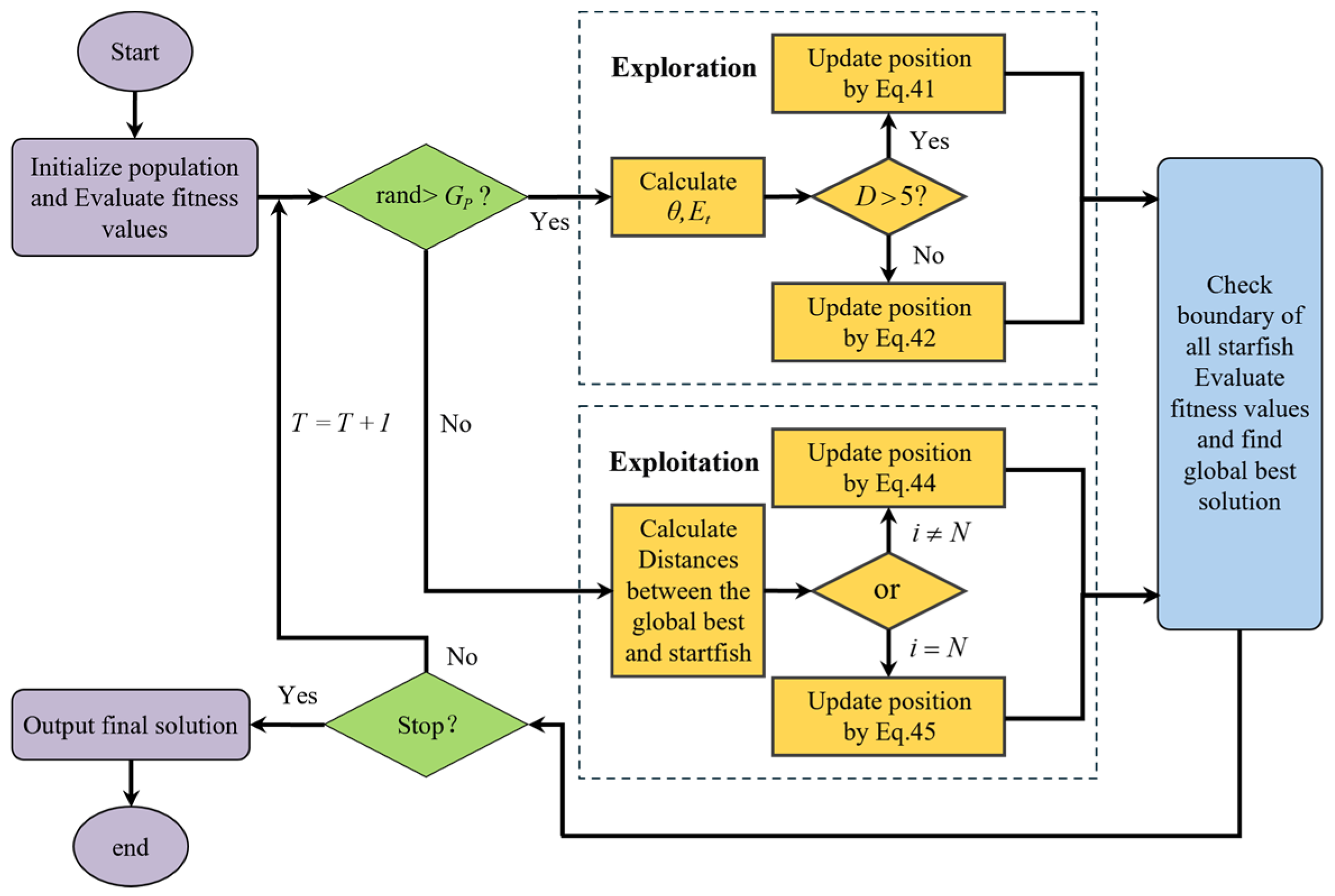
• Step 1: In the initialization phase, set a reasonable population size, i.e., the number of starfish and the maximum number of iterations. Randomly generate the corresponding number of population matrices under the boundary constraints (i.e., within the HPR ellipse region). Calculate the initial fitness values (i.e., FOV coverage) of all starfish according to the objective function. Then, enter it into the algorithm’s main loop.
• Step 2: According to the random number to determine whether to enter the exploration or development phase, this is represented as $G_p=0.5$ in Figure 7, indicating that the algorithm sets the probability of the exploration and development phases to be the same, with balance.
• Step 3: Enter the exploration phase. The algorithm designs two starfish position updating rules based on different dimensions to satisfy different sizes of the search space and improve the exploration efficiency. For the coverage optimization problem, when the number of fields of view is greater than five, the starfish position is updated by Equation (41), and the updated FOV coverage is calculated; when the number of fields of view is less than or equal to 5, it is updated by Equation (42).
• Step 4: Enter the development phase. The algorithm adopts a parallel bidirectional search strategy, which enhances the development of the optimization problem, overcomes the local optimality problem, and facilitates the coverage optimization problem to seek the optimal solution in all regions of the target HPR.
• Step 5: The conditional termination phase continuously evaluates the current optimal positions of all the starfish and calculates the corresponding optimal solution, i.e., iterates the value of the FOV coverage through the two balanced parallel sessions of exploration and exploitation. When the maximum number of iterations is satisfied, the loop is stopped, and the final global optimal solution and the best position of the starfish, i.e., the maximum FOV coverage and the corresponding FOV center coordinates, are output.

4. Simulation Analysis

Set the predicted duration of 100 s as the handover time for midcourse–terminal guidance. Using the parameterized error-bounded pipeline model from Section 2.2, recursively calculate the spatial range of the target HPR at this moment. Select the latitude error and altitude error corresponding to the 100 s prediction duration in Table 2 as the semi-major and semi-minor axes of the target HPR ellipse in the 2D plane. Further, define the maximum detection range of the interceptor seekers $R_{\max }$ as 60 km and the FOV angle $\varphi$ as 5°. Under these constraints, conduct a simulation experiment for multi-interceptor detection FOV coverage optimization using SFOA.

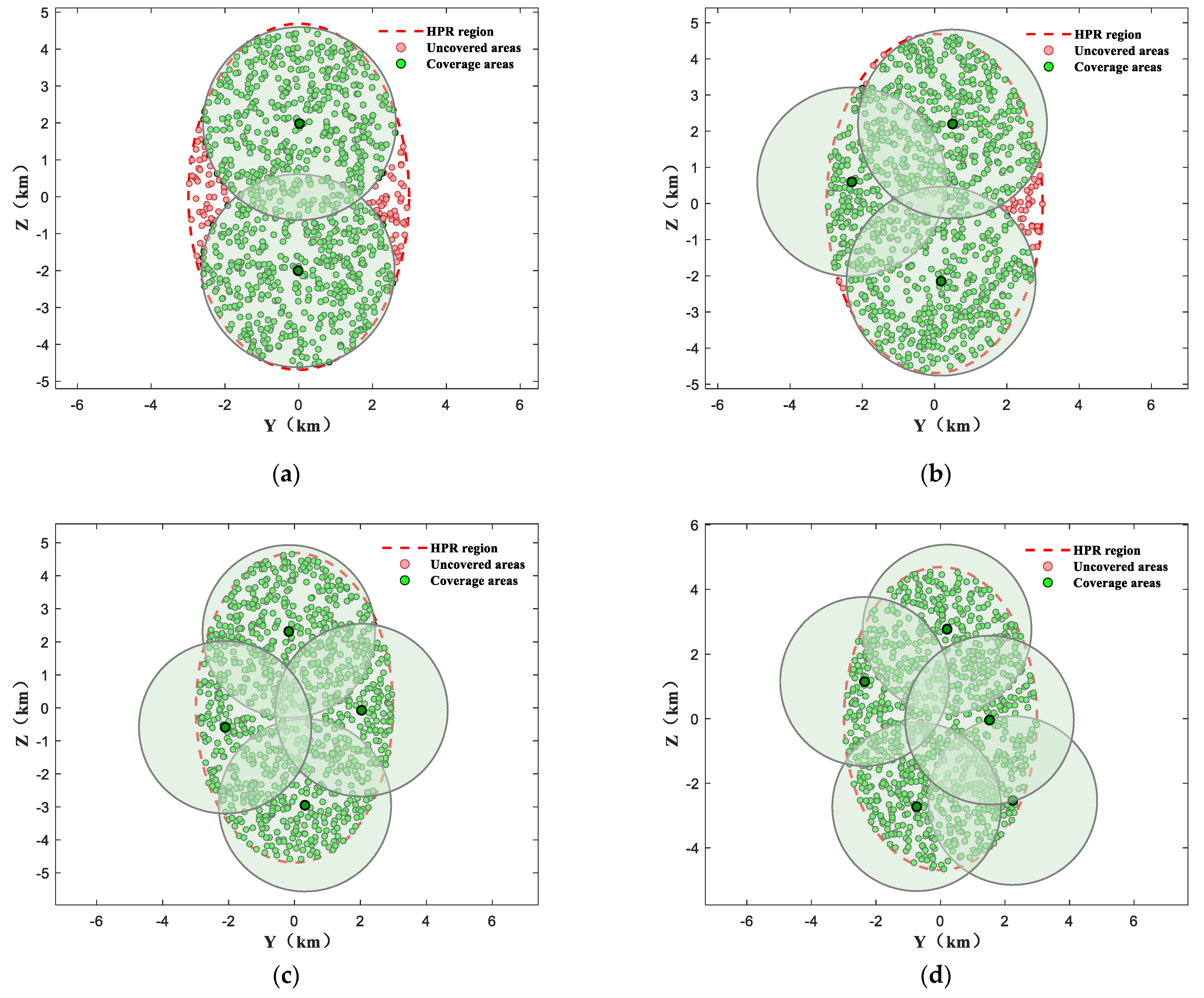
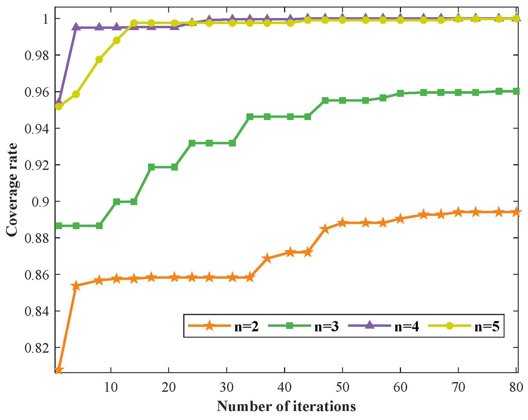
4.1. Coverage Optimization Simulation with Different Numbers of Interceptors

This group of experiments investigates the coverage optimization of a single target HPR space using different interceptor quantities. The aim is to validate the feasibility and effectiveness of the proposed model and algorithm. Under relevant constraints, the minimum number of interceptors required to thoroughly cover the target HPR space is analyzed. This parameter is critical for optimizing collaborative detection strategies and enhancing target acquisition efficiency. The simulation conditions and experimental data are detailed in

Table 5. Coverage optimization simulation experiment conditions with different numbers of interceptors.

Simulation Conditions	Parameter Settings
Population size of SFOA	15
Iterations of SFOA	80
Range of HPR	latitudinal error Y ≈ 2.99 km, orientation error Z ≈ 4.69 km
Diameter of FOV	L ≈ 5.23 km
Number of interceptors	M = [2, 3, 4, 5]

and

Table 6. Coverage optimization simulation experiment data with different numbers of interceptors.

Serial No.	No. of Interceptors	Coverage Rate	Convergence Time	Relative Center of FOV
1	2	89.0%	0.170 s	(−0.0177, −2.0032) (0.0204, 1.9827)
2	3	96.0%	0.220 s	(−2.2927, 0.5971) (0.1789, −2.1483) (0.4959, 2.1983)
3	4	100%	0.292 s	(0.3164, −2.9508) (−0.1732, 2.3160) (2.0324, −0.0715) (−2.1023, −0.5872)
4	5	100%	0.268 s	(2.2424, −2.5345) (−0.7378, −2.7265) (0.2049, 2.7718) (−2.3531, 1.1493) (1.5194, −0.0433)

, respectively, with coverage results illustrated in Figure 8.

Under the constraints listed in Table 5, this experiment solves the coverage optimization problem for varying interceptor quantities using the SFOA algorithm. As shown in Figure 8, the combined FOV formed through dynamic stitching and superposition of multiple seeker FOVs achieves fundamental coverage of the single-target HPR. Through iterative optimization, maximum coverage is attained while resolving the central illumination point coordinates of each seeker FOV in the target HPR coordinate system. Quantitative results in Figure 9 and Table 5 demonstrate that as the interceptor count increases from 2 to 4, the coverage rate rises steadily from 89% to 100%, with the convergence time slightly increasing from 0.170 s to 0.292 s. The result preliminarily validates the feasibility and effectiveness of the coverage model and SFOA algorithm. Notably, when the interceptor count expands to 5, the coverage rate remains saturated at 100% with significant FOV redundancy, while the convergence time decreases marginally by 0.024 s. The result indicates that redundant exploration for coverage enhancement is unnecessary under saturation conditions, thereby reducing computational overhead. The experiment also references the minimum interceptors required for full HPR coverage: under the given constraints, four interceptors achieve complete HPR coverage with optimal cost-effectiveness.

From an overall performance perspective, the algorithm exhibits an average convergence time of 0.2375 s. In a dynamic scenario with a relative velocity of 2000 m/s, the spatial scale of the solution domain is approximately 475 m—two orders of magnitude smaller than the physical scale of the seeker detection FOV range (80 km). The algorithm demonstrates favorable rapid convergence characteristics, preliminarily satisfying online computational requirements while adapting to the time-varying nature of the target HPR. Furthermore, the optimized illumination center coordinates of each seeker FOV provide essential terminal constraints for interceptor guidance.

4.2. Coverage Optimization Simulation Under Time-Varying Target HPR

To further verify the coverage optimization ability and convergence speed of the proposed model and algorithm for the time-varying features of the target HPR, two groups of simulation experiments are designed: the first group takes the three interceptors as the benchmarks and selects 20 sets of the target HPR datasets with different amplitudes to carry out the coverage ability test, and quantitatively analyzes the coverage index and the convergence speed parameters. Among them, to select a reasonable amplitude span, the 75 s prediction error pipeline distribution data are superimposed as the benchmark so that the total amplitude span of the target HPR corresponds to the latitudinal and skyward error values of prediction duration 75~150 s in Table 4; the second group takes the 95% coverage threshold as the constraint and focuses on evaluating the convergence speed index by adjusting the number of interceptors to match the time-varying size of the target HPR. The relevant simulation experiment conditions are shown in

Table 7. Coverage optimization simulation experiment conditions under time-varying target HPR.

Simulation Conditions	Parameter Settings
Range of HPR	Latitudinal error Y ≈ 2.25 km, Skyward error Z ≈ 3.53 km At 0.1 km/trip, accumulate 20 times
FOV diameter	L ≈ 5.23 km
Number of interceptors	First group M = 3; Second group M adapted
coverage rate	Second group ≥ 95%

.

The results of the first simulation group (

Table 8. The first group of simulation experiment data.

Serial No.	Range of HPR	Coverage Rate	Convergence Time
1–4	Y = 2.2–2.5, Z = 3.5–3.8	100%	0.13 s
5	Y = 2.6, Z = 3.9	99.91%	0.15 s
6	Y = 2.7, Z = 4.0	99.54%	0.15 s
7	Y = 2.8, Z = 4.1	98.84%	0.16 s
8	Y = 2.9, Z = 4.2	97.83%	0.16 s
9	Y = 3.0, Z = 4.3	96.70%	0.17 s
10	Y = 3.1, Z = 4.4	95.15%	0.18 s
11	Y = 3.2, Z = 4.5	93.84%	0.19 s
12	Y = 3.3, Z = 4.6	92.48%	0.19 s
13	Y = 3.4, Z = 4.7	90.82%	0.20 s
14	Y = 3.5, Z = 4.8	89.25%	0.21 s
15	Y = 3.6, Z = 4.9	87.64%	0.23 s
16	Y = 3.7, Z = 5.0	86.19%	0.23 s
17	Y = 3.8, Z = 5.1	84.40%	0.23 s
18	Y = 3.9, Z = 5.2	82.80%	0.25 s
19	Y = 4.0, Z = 5.3	80.36%	0.27 s
20	Y = 4.1, Z = 5.4	79.46%	0.26 s

and Figure 10) indicate that as the target HPR magnitude increases, the coverage rate gradually declines from 100% to 79.46%. At the same time, the convergence time rises from 0.13 s to 0.26 s. The average coverage rate is 92.76 ± 7.17%, and the average convergence time is 0.19 ± 0.05 s. Figure 10 shows concentrated distributions of the 20 datasets in the convergence time–coverage rate coordinate system, demonstrating stable solving performance, rapid convergence, and robust adaptability to varying HPR magnitudes. Table 8 further reveals that larger HPR magnitudes correlate with longer convergence times, attributable to the algorithm’s expanded spatial search for optimal solutions.

Based on the first group’s results, the second simulation group sets a ≥95% coverage rate as the threshold for successful target acquisition during the handover phase. Interceptor quantities are dynamically adjusted across 20 HPR ranges to maintain coverage above 95%, validating the model’s capability under multivariate coupling conditions (

Table 9. The second group of simulation experiment data.

Serial No.	Numbers	Range of HPR	Coverage Rate	Time
1–6	3	Y = 2.25~2.75, Z = 3.53~4.03	97.0~100%	0.14~0.17 s
7–9	4	Y = 2.85~3.05, Z = 4.13~4.33	96.6~99.1%	0.14~0.19 s
10	5	Y = 3.15, Z = 4.43	96.2%	0.15 s
11–17	6	Y = 3.25~3.85, Z = 4.53~5.13	96.8~100%	0.15~0.18 s
18	7	Y = 3.95, Z = 5.23	96.4%	0.18 s
19–20	8	Y = 4.05~4.15, Z = 5.33~5.43	96.9~98.4%	0.19~0.20 s

, Figure 11).

In the second set of simulation experiments, the data shown in Table 8 and the data distribution in Figure 11 indicate that the proposed model and algorithm can adapt to the multivariate coupling condition of matching changes in the time-varying HPR and the number of interceptors to achieve more than 95% of the coverage target and have the ability to cope with the time-varying characteristics of the target HPR. Specifically, through 20 groups of experiments, the number of interceptors is increased from three to eight to adapt to the target HPR’s incremental changes; the average convergence time is 0.17 ± 0.02 s, the average coverage rate is 98.7 ± 0.03%, and the overall coverage redundancy is small, reflecting a better cost-effective function. The relatively centralized location of the experimental data points in each group also indicates that the proposed model and algorithm are stable and rapid in controlling the convergence time and adjusting the number of interceptors and have good adaptability. In addition, the results of this experiment have some reference value for determining the number of interceptors, formation adjustment, and topology optimization for cooperative detection.

5. Conclusions

To address the challenges of target HPR detection and capture at midcourse–terminal guidance handover in CDUAV, this paper proposes a collaborative multi-interceptor detection coverage optimization method based on predictive error pipeline modeling. The main conclusions are as follows: (1) In terms of target HPR range estimation, a parametric modeling method based on error transfer theory is innovatively proposed which realizes error transfer and accumulation through the equations of motion and combines with a small-sample t-distribution to construct a prediction error pipeline. The simulation shows that the method shortens the prediction error convergence time from 15.82 s to 0.09 s compared with the Monte Carlo simulation, and the confidence interval of the error pipeline envelope is 99%, significantly improving the ability to reflect the real trajectory. It also reveals that the target HPR patterns are closer to the ellipsoid. (2) In terms of cooperative detection coverage optimization, an optimization framework containing the target HPR model, the FOV model, and the FOV coverage as the objective function is established. It is verified by simulation that when the handover window moment is 100 s, three interceptors can achieve a 96% coverage rate, and the average convergence time is 0.2375 s. (3) In terms of the method applicability, the simulation analysis shows that when the number of interceptors is three, the target HPR time-variation leads to the decrease in the coverage rate from 100% to 79.46%, and the convergence time is increased from 0.13 s to 0.26 s, and the average coverage of 92.76 ± 7.17%; dynamically adjusting the number of interceptors can maintain more than a 95% coverage rate, with an average coverage rate of 98.7 ± 0.03% and a convergence time of 0.17 ± 0.02 s, which verifies the robustness and adaptability of the method. The method in this paper provides new ideas for solving the HPR estimation of the mid–end guided handover target and the cooperative detection problem of interceptors, focusing on constructing a solution framework for the CDUAV cooperative detection coverage optimization problem. The focus of this paper is to verify the feasibility and effectiveness of the method, and the influence of disturbance factors is not considered at the current stage. Specifically, the disturbance in the error pipeline modeling mainly comes from environmental factors (e.g., atmospheric disturbances, etc.), and although it will introduce additional error components, its impact is relatively limited and does not affect the dominant modal characteristics of the error transmission; the disturbance in the FOV modeling is mainly manifested in the form of active disturbances, which have a more significant impact on the detection distance and capture probability, and disturbances with different orientations will lead to distortions of the FOV shape. This type of disturbance has a more significant effect on the detection distance and capture probability, and different orientations will lead to the distortion of the FOV shape. It should be noted that when these disturbance factors are introduced, the coverage optimization problem will evolve into a complex multi-objective optimization problem, which will be the direction of this study.

References

- Ding, Y.B.; Yue, X.K.; Chen, G.S.; Si, J.S. Review of control and guidance technology on hypersonic vehicle. Chin. J. Aeronaut. 2022, 35, 1–18. [Google Scholar] [CrossRef]
- Fan, Y.; Lu, F.; Zhu, W.X.; Bai, G.Z.; Yan, L. A Hybrid Model Algorithm for Hypersonic Glide Vehicle Maneuver Tracking Based on the Aerodynamic Model. Appl. Sci. 2017, 7, 159. [Google Scholar] [CrossRef]
- Liu, F.R.; Lu, L.N.; Zhang, Z.H.; Xie, Y.; Chen, J. Intelligent Trajectory Prediction Algorithm for Hypersonic Vehicle Based on Sparse Associative Structure Model. Drones 2024, 8, 505. [Google Scholar] [CrossRef]
- Jeon, B.J.; Bang, J.; Park, B.G.; Ahn, J.; Tahk, M.J. Guidance scheme for operating multiple ship defense missiles with dual seekers. Proc. Inst. Mech. Eng. Part G J. Aerosp. Eng. 2016, 230, 601–614. [Google Scholar] [CrossRef]
- Kang, H.L.; Wang, P.Y.; Song, S.M. A generalized three-dimensional cooperative guidance law for various communication topologies with field-of-view constraint. Proc. Inst. Mech. Eng. Part G J. Aerosp. Eng. 2023, 237, 2353–2369. [Google Scholar] [CrossRef]
- Lee, C.H.; Hyun, C.; Lee, J.G.; Choi, J.Y.; Sung, S. A Hybrid Guidance Law for a Strapdown Seeker to Maintain Lock-on Conditions against High Speed Targets. J. Electr. Eng. Technol. 2013, 8, 190–196. [Google Scholar] [CrossRef]
- Li, F.; Xiong, J.J.; Lan, X.H.; Bi, H.K.; Chen, X. NSHV trajectory prediction algorithm based on aerodynamic acceleration EMD decomposition. J. Syst. Eng. Electron. 2021, 32, 103–117. [Google Scholar] [CrossRef]
- Maeder, U.; Morari, M.; Baumgartner, T.I. Trajectory Prediction for Light Aircraft. J. Guid. Control Dyn. 2011, 34, 1112–1119. [Google Scholar] [CrossRef]
- Ren, J.H.; Wu, X.; Liu, Y.; Ni, F.; Bo, Y.M.; Jiang, C.H. Long-Term Trajectory Prediction of Hypersonic Glide Vehicle Based on Physics-Informed Transformer. IEEE Trans. Aerosp. Electron. Syst. 2023, 59, 9551–9561. [Google Scholar] [CrossRef]
- Wei, X.Q.; Gu, L.F.; Li, R.K.; Wang, S.Y. Trajectory Tracking and Prediction of Hypersonic Vehicle Based on Singer Model. Aerosp. Control 2017, 35, 62–66+72. (In Chinese) [Google Scholar] [CrossRef]
- Li, F.; Xiong, J.J.; Lan, X.H.; Bi, H.K.; Tan, X.S. Hypersonic Vehicle Trajectory Prediction Algorithm Based on Hough Transform. Chin. J. Electron. 2021, 30, 918–930. [Google Scholar] [CrossRef]
- Sun, L.H.; Yang, B.Q.; Ma, J. Trajectory prediction in pipeline form for intercepting hypersonic gliding vehicles based on LSTM. Chin. J. Aeronaut. 2023, 36, 421–433. [Google Scholar] [CrossRef]
- Zhai, D.L.; Lei, H.M.; Li, J.; Liu, T. Trajectory prediction of hypersonic vehicle based on adaptive IMM. Acta Aeronaut. Et Astronaut. Sin. 2016, 37, 3466–3475. (In Chinese) [Google Scholar]
- Hu, Y.D.; Gao, C.S.; Li, J.L.; Jing, W.X.; Li, Z. Novel trajectory prediction algorithms for hypersonic gliding vehicles based on maneuver mode on-line identification and intent inference. Meas. Sci. Technol. 2021, 32, 115012. [Google Scholar] [CrossRef]
- Yoon, S.; Jang, D.; Yoon, H.; Park, T.; Lee, K. GRU-Based Deep Learning Framework for Real-Time, Accurate, and Scalable UAV Trajectory Prediction. Drones 2025, 9, 142. [Google Scholar] [CrossRef]
- Lu, S.N.; Qian, Y. Enhanced Trajectory Forecasting for Hypersonic Glide Vehicle via Physics-Embedded Neural ODE. Drones 2024, 8, 377. [Google Scholar] [CrossRef]
- Procházka, O.; Novák, F.; Báca, T.; Gupta, P.M.; Penicka, R.; Saska, M. Model predictive control-based trajectory generation for agile landing of unmanned aerial vehicle on a moving boat. Ocean Eng. 2024, 313, 119164. [Google Scholar] [CrossRef]
- Hu, X.; Wang, X.; Jiang, X.; Wang, Z.; Qin, S.; Lai, J. Uncertain trajectory prediction of hypersonic flight vehicles based on Gaussian process regression. Aerosp. Technol. 2022, 4, 49–61. (In Chinese) [Google Scholar] [CrossRef]
- Li, M.J.; Zhou, C.J.; Shao, L.; Lei, H.M. An Intelligent Trajectory Prediction Algorithm for Hypersonic Glide Targets Based on Maneuver Mode Identification. Int. J. Aerosp. Eng. 2022, 2022, 1–17. [Google Scholar] [CrossRef]
- Lee, S.; Ann, S.; Cho, N.; Kim, Y. Capturability of Guidance Laws for Interception of Nonmaneuvering Target with Field-of-View Limit. J. Guid. Control Dyn. 2019, 42, 869–884. [Google Scholar] [CrossRef]
- Liu, S.; Lin, Z.; Huang, W.; Yan, B. Technical Development and Future Prospects of Cooperative Terminal Guidance Based on Knowledge Graph Analysis: A Review. J. Zhejiang Univ.-Sci. A 2024, in press. [Google Scholar]
- Liu, S.X.; Lin, Z.H.; Huang, W.; Yan, B.B. Current development and future prospects of multi-target assignment problem: A bibliometric analysis review. Def. Technol. 2025, 43, 44–59. [Google Scholar] [CrossRef]
- Zheng, Z.; Cai, S.C. A collaborative target tracking algorithm for multiple UAVs with inferior tracking capabilities. Front. Inf. Technol. Electron. Eng. 2021, 22, 1334–1350. [Google Scholar] [CrossRef]
- Zhou, M.; Li, J.Y.; Wang, C.; Wang, J.; Wang, L. Applications of Voronoi Diagrams in Multi-Robot Coverage: A Review. J. Mar. Sci. Eng. 2024, 12, 1022. [Google Scholar] [CrossRef]
- Drezner, T.; Drezner, Z. Voronoi diagrams with overlapping regions. OR Spectr. 2013, 35, 543–561. [Google Scholar] [CrossRef]
- Zhou, J.; Lei, H.M. Coverage-based cooperative target acquisition for hypersonic interceptions. Sci. China Technol. Sci. 2018, 61, 1575–1587. [Google Scholar] [CrossRef]
- Luo, C.X.; Zhou, C.J.; Bu, X.W. Multi-Missile Phased Cooperative Interception Strategy for High-Speed and Highly Maneuverable Targets. IEEE Trans. Aerosp. Electron. Syst. 2025, 61, 1971–1996. [Google Scholar] [CrossRef]
- Chaturvedi, P.; Daniel, A.K. A Comprehensive Review on Scheduling Based Approaches for Target Coverage in WSN. Wirel. Pers. Commun. 2022, 123, 3147–3199. [Google Scholar] [CrossRef]
- Lee, J.W.; Lee, J.J. Ant-Colony-Based Scheduling Algorithm for Energy-Efficient Coverage of WSN. IEEE Sens. J. 2012, 12, 3036–3046. [Google Scholar] [CrossRef]
- Yue, Y.G.; Cao, L.; Zhang, Y. Novel WSN Coverage Optimization Strategy Via Monarch Butterfly Algorithm and Particle Swarm Optimization. Wirel. Pers. Commun. 2024, 135, 2255–2280. [Google Scholar] [CrossRef]
- Zhu, C.; Zheng, C.L.; Shu, L.; Han, G.J. A survey on coverage and connectivity issues in wireless sensor networks. J. Netw. Comput. Appl. 2012, 35, 619–632. [Google Scholar] [CrossRef]
- Deif, D.S.; Gadallah, Y. Classification of Wireless Sensor Networks Deployment Techniques. IEEE Commun. Surv. Tutor. 2014, 16, 834–855. [Google Scholar] [CrossRef]
- Anusuya, P.; Vanitha, C.N.; Cho, J.H.Y.; Easwaramoorthy, S.V. A comprehensive review of sensor node deployment strategies for maximized coverage and energy efficiency in wireless sensor networks. Peerj Comput. Sci. 2024, 10, e2407. [Google Scholar] [CrossRef]
- Zhang, B.L.; Zhou, D.; Li, J.L.; Yao, Y.H. Coverage-Based Cooperative Guidance Strategy by Controlling Flight Path Angle. J. Guid. Control Dyn. 2022, 45, 972–981. [Google Scholar] [CrossRef]
- Zhai, C.; He, F.H.; Hong, Y.G.; Wang, L.; Yao, Y. Coverage-Based Interception Algorithm of Multiple Interceptors Against the Target Involving Decoys. J. Guid. Control Dyn. 2016, 39, 1646–1652. [Google Scholar] [CrossRef]
- Su, W.S.; Li, K.B.; Chen, L. Coverage-based three-dimensional cooperative guidance strategy against highly maneuvering target. Aerosp. Sci. Technol. 2019, 85, 556–566. [Google Scholar] [CrossRef]
- Li, J.; He, Y.C.; Shao, L.; Feng, X.H. Reentry glide vehicle trajectory prediction method via multidimensional intention fusion. Aerosp. Sci. Technol. 2025, 159, 109960. [Google Scholar] [CrossRef]
- Wang, H.J.; Lei, H.M.; Zhang, D.Y.; Zhou, J.; Shao, L. Midcourse and terminal guidance handover window for interceptor against near space hypersonic target. J. Natl. Univ. Def. Technol. 2018, 40, 1–8. (In Chinese) [Google Scholar]
- Jia, H.M.; Meng, B.; Wei, Y.H.; Li, S.L. Improved arithmetic optimization algorithm for wireless sensor network coverage. J. Minnan Norm. Univ. Nat. Sci. 2022, 35, 54–61. (In Chinese) [Google Scholar] [CrossRef]
- Izci, D.; Ekinci, S.; Jabari, M.; Bajaj, M.; Blazek, V.; Prokop, L.; Yildiz, A.R.; Mirjalili, S. A new intelligent control strategy for CSTH temperature regulation based on the starfish optimization algorithm. Sci. Rep. 2025, 15, 12327. [Google Scholar] [CrossRef]