Stochastic Planning of Synergetic Conventional Vehicle and UAV Delivery Operations

Abstract

Synergetic transportation schemes are extensively used in package delivery operations, exploiting the best features of different modes. This paper proposes a methodology to solve the mode assignment and routing problem for the case of combined conventional vehicle and unmanned aerial vehicle (CV–UAV) parcel deliveries under uncertainty for next-day operations. This research incorporates ground and air uncertainties: travel times are assumed for conventional vehicles, while UAV paths are affected by weather conditions and restricted flying zones. A nested genetic algorithm is initially used to solve the problem under fixed conditions. Then, a robust optimization approach is employed to propose the best solution that will perform well in a stochastic environment. The framework is applied to a case study of realistic urban–suburban size, and results are discussed. The entire platform is useful for strategic decisions on infrastructure and for operation planning with satisfactory performance and less risk.

1. Background

The use of unmanned aerial vehicles (UAVs) in transport has been extensively investigated regarding safety and operational efficiency. Based on current technology concerning weight-carrying capabilities and range, small-package deliveries have been the primary application. Remote locations with limited accessibility are expected to benefit from such operations, while last-mile services can be optimized [1,2]. UAVs benefit from not requiring an established ground network; however, airspace also presents obstacles, be it no-fly zones (such as airports or military zones) or just the weather [3].

Combined operations of conventional vehicles (CVs) and UAVs have been proposed in various forms. One of the most cited works is that of Murray and Chu [4], who introduced the “Flying Sidekick Traveling Salesman Problem” (FSTSP). Parcels can be delivered either by truck or UAV, the latter being able to launch from the truck or the depot to customers and return to a different location, where it meets the truck again for recovery. UAVs fly straight within their operational range. Similar setups have been proposed by others, sometimes considering identical take-off and landing locations [5], compulsory truck deliveries while on the truck’s path [6], or on-route UAV deployment [7]. Macrina et al. [8] explored the efforts made to date, highlighting areas for further research, such as the inclusion of real-life variables and stochastic conditions.

Real-life limitations in infrastructure and conditions, as well as the stochastic nature of such operations and inherent risks, have received comparatively little attention when specifically considering combined CV–UAV operations. In terms of vehicle routing alone, research on seeking a robust solution under uncertainty is not new. Gendreau et al. [9] sampled several stochastic VRP cases, citing uncertainty sources in demand, travel times, and customers. Bertsimas and Simchi-Levi [10] highlighted the importance of including congestion and stochasticity in the VRP problems and evaluated relevant heuristic algorithms. Wu and Hifi [11] proposed a scenario-based optimization process through a custom robust model, also using a guided neighborhood search-based heuristic to evaluate the results. A chance-constrained approach was also applied by Kepaptsoglou et al. [12], where stochastic weather conditions and affected travel times for ships were assumed. Airspace constraints and uncertainties have also been a matter of ongoing research, mostly treating adverse condition areas as obstacles of various forms and intensities [13,14]. For routing optimization purposes, multi-agent reinforcement learning techniques were used by Zhang et al. [15], while mathematical and heuristic models were the approach assumed by [16]. Wang and Zhao [17] tackled rescheduling for a fleet of heterogeneous drones through a genetic algorithm. Travel time uncertainties were considered by [18] and a branch-and-price algorithm was used for optimization, while the stochastic nature of the problem was also a study subject for Tolooie et al. [19], who employed mixed-integer programming for the solution.

Deng et al. [20] followed a Benders decomposition approach to solve stochastic truck-and-drone routing problems with risk minimization, while vehicle and drone restricted areas were considered in the work of Wei et al. [21], who proposed a hybrid genetic algorithm and variable neighborhood search with a learning mechanism. Mahmoodi et al. [22] focused on multi-objective optimization, after introducing constraints and special parameters in the areas of pick-up, time windows, and battery charging. Zhang et al. [23] focused on finding an exact solution to the truck–drone routing problem, minimizing cost and time. A systematic risk model was elaborated by Wang et al. [24], who offered a risk optimization method for hybrid truck–drone last-mile deliveries. Gonzalez et al. [25] expanded the field of research into truck–drone team logistics, and a greedy heuristic was coded, also using a simulated annealing algorithm for global optimization purposes.

This research specifically explores the areas of stochastic optimization, providing a new framework to assist risk-balanced decision-making for next-day operations. We tackle realistic situations that the logistics ecosystem faces worldwide, assuming uncertainty both on the ground and in the air. Unlike previous studies that typically address either ground-based or airspace uncertainty in isolation, this work simultaneously incorporates stochastic variability in both traffic conditions and UAV flight feasibility. By employing a scenario-based robust optimization framework across the multimodal system, it achieves a risk-balanced operational plan capable of adapting to varying ground and air conditions. This integrated modeling approach advances the state of the art by bridging the gap between separate uncertainty dimensions, enabling more resilient and realistic next-day planning for hybrid CV–UAV delivery operations.

2. Problem Description

2.1. Basic Problem and Assumptions

Multiple items need to be transported from the central depot (CD) to customers located at various delivery locations (DLs). The items can be delivered to the DLs either by a conventional vehicle (CV) or an unmanned aerial vehicle (UAV). The CV follows a fixed network for transportation, while UAVs offer more flexibility but have limitations in terms of range and are required to navigate around potential no-fly zones and adverse weather conditions. UAVs can be launched and recovered by trucks at designated safe locations (virtual hubs, or VHs) or by personnel (at the CD and other remote depots, or RDs, throughout the CV network). The conditions along the fixed network are uncertain, although historical patterns have been observed. The weather forecast is also probabilistic. Each item is assigned to a specific mode of transportation for either the final segment or the entire journey. UAVs can only be launched or recovered at allowed locations throughout the network. Operations planning requires a decision on the mode assignment for each item, the nodes used for UAV deployment, and the order of visit of critical nodes. The solution should be able to perform well under a spectrum of expected conditions.

2.2. Description of Constraints

To accurately model the proposed delivery system, the following operational assumptions and constraints are established:

-

Operations involve a single CV departing from the CD. The CV is assumed to have sufficient capacity to carry all assigned parcels and UAV units.

-

UAVs are of the vertical take-off and landing (VTOL) type.

-

Each DL may be visited once for either direct delivery, UAV deployment, or both, although it remains accessible multiple times for routing purposes.

-

The CV tour begins and concludes with the CD.

-

The CV can serve multiple DLs in sequence.

-

Each UAV is restricted to transporting a single parcel per mission.

-

UAVs complete one outbound and one inbound trip per deployment cycle.

-

Multiple UAVs can be simultaneously deployed from a single point, following preparation.

-

UAVs must return to the same launch point after completing their delivery.

-

RDs can launch UAVs independently, without requiring the CV to remain onsite during their return, although a fixed trans-shipment time is incurred.

-

UAVs launched from the DL do not impose a waiting or trans-shipment time on the CV.

-

Each item is limited to a single transfer between vehicles throughout its journey.

2.3. Stochastic Conditions

2.3.1. Conventional Vehicle Network

Conditions throughout the conventional vehicle network (CVN) are uncertain, but historical patterns help with prediction. Link travel times are stochastic variables, based on the link’s respective CV travel speed; this refers to the representative average speed throughout the entire link length, observed at a mesoscopic level. Historical values are used to extract a distribution of mean speed for each link. While planning the operations, it is assumed that conditions at each link will fall within an expected range and according to its observed speed distribution.

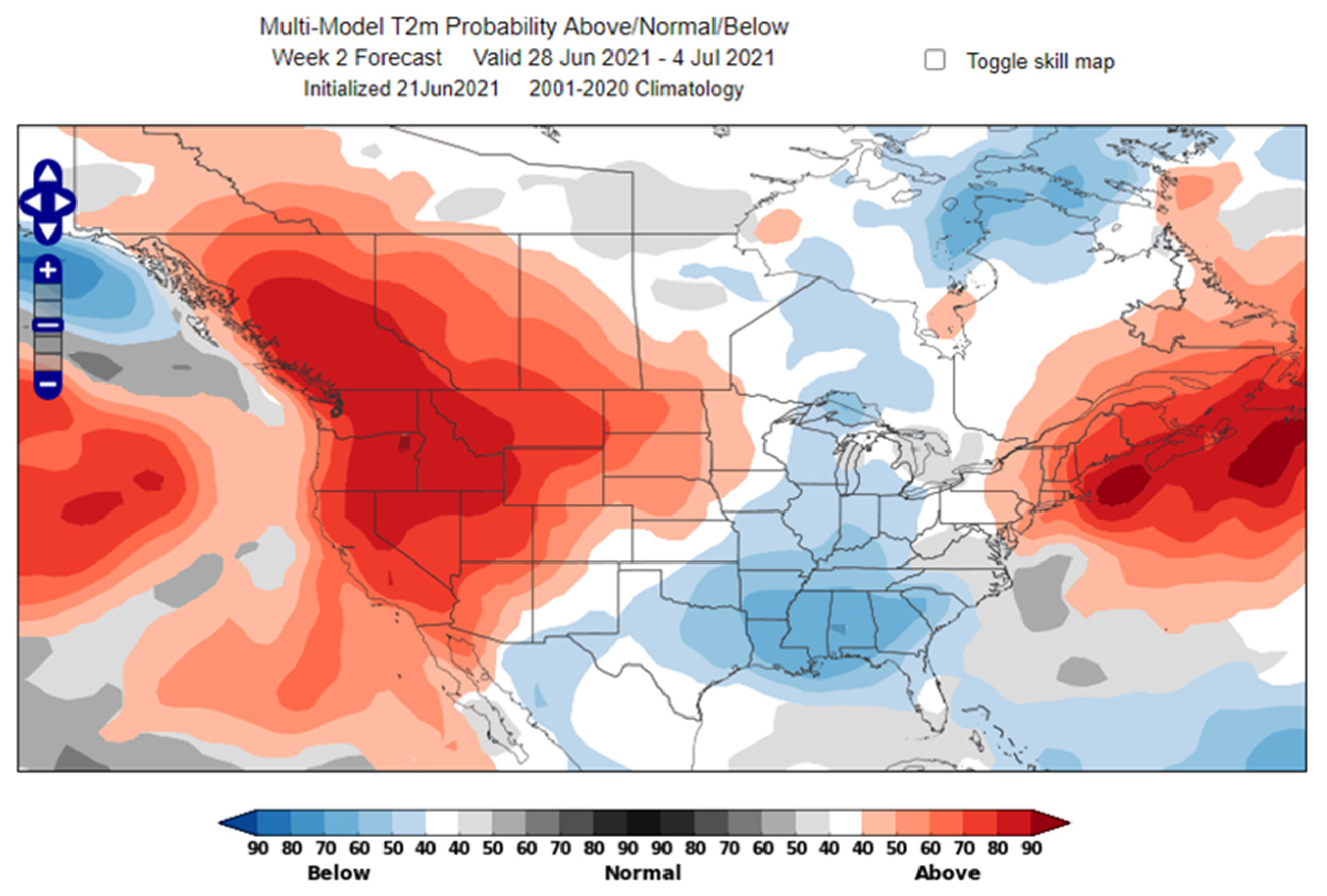
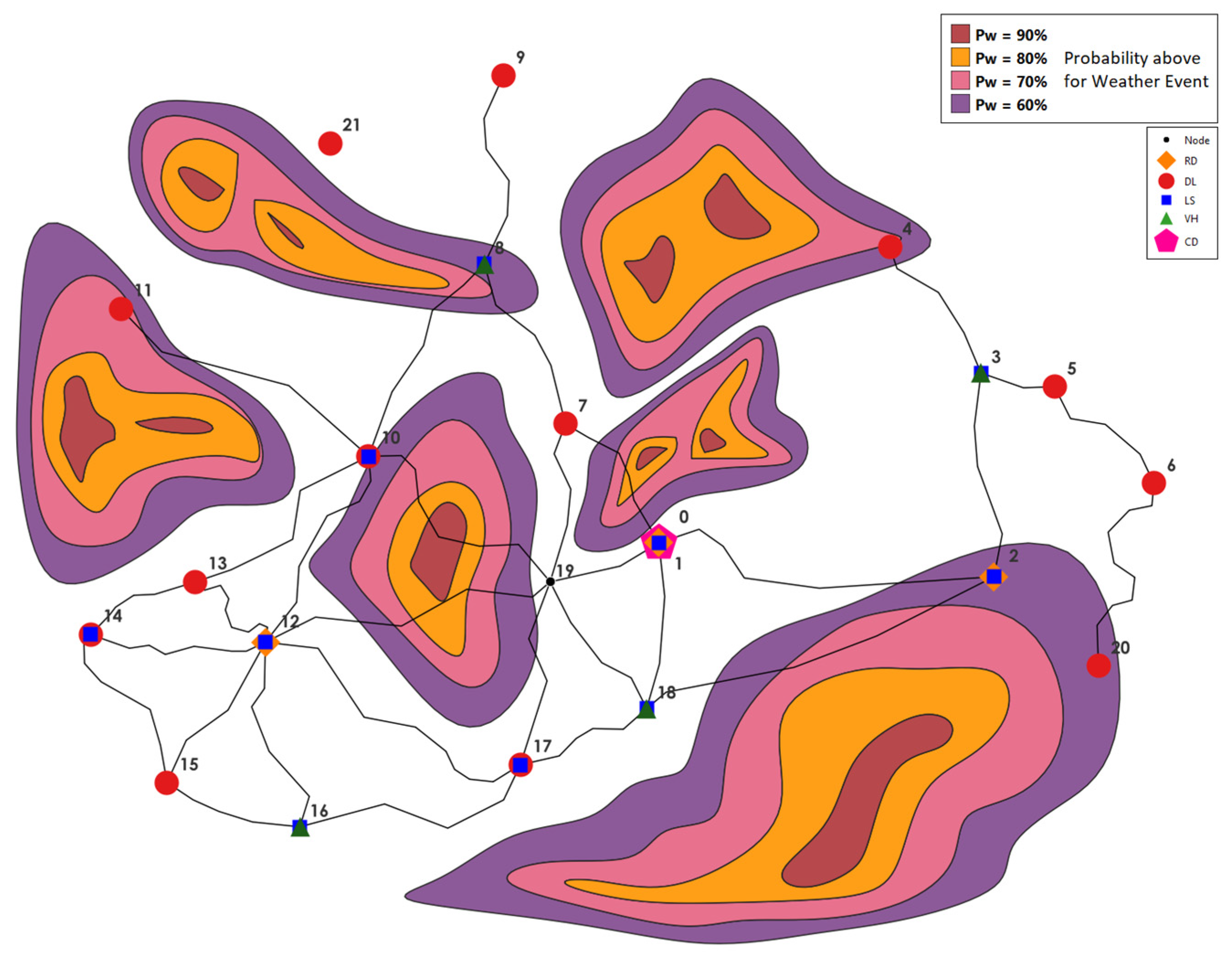
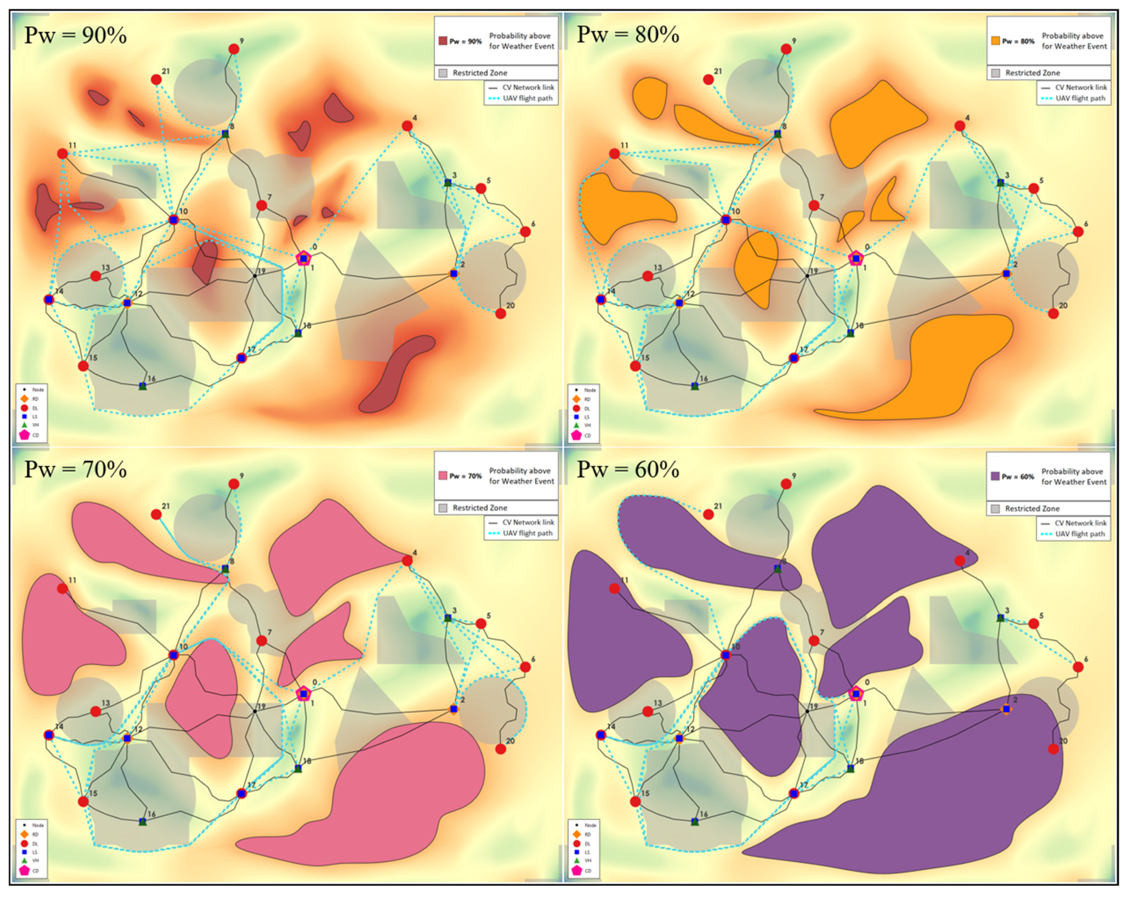
2.3.2. Weather Forecast

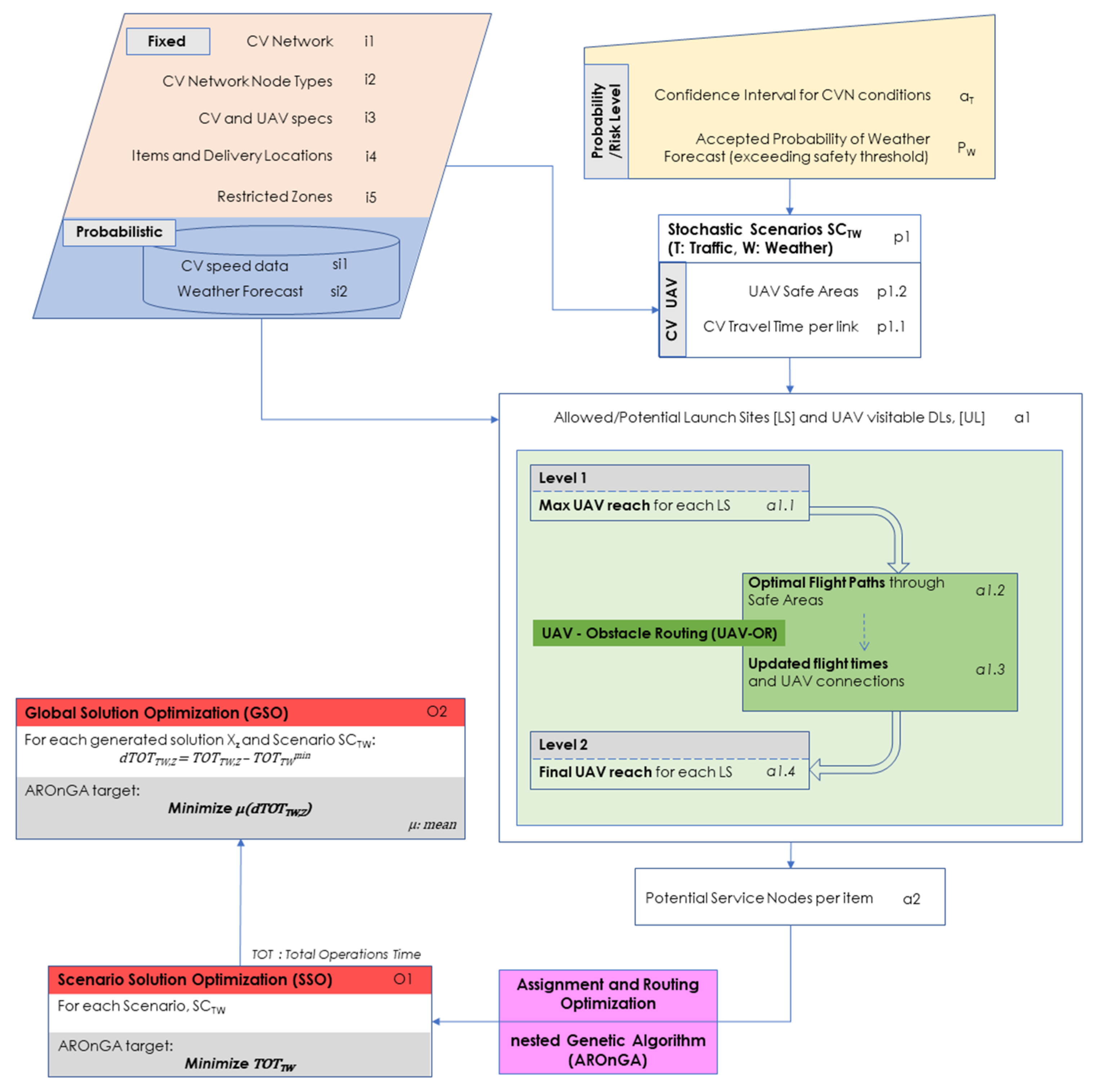
The weather forecast is given in the form of a probabilistic prediction on whether a certain threshold is surpassed; this could be rain intensity or wind speed exceeding UAV capabilities at any time within the expected duration of operations. We are referring to a dichotomous event (e.g., rain exceeds a certain value or not), given as a forecast at m categories of probability, namely polychotomous forecasts [26]. To acquire a probability forecast, we divide the potential outcomes into ranges or bins and assign a probability of occurrence to each bin. This information does not tell us precisely what, i.e., the rain intensity, will be, but it is highly likely to be above or below a certain value [27]. The following Figure 1 depicts an example of such a forecast.

3. Methodology

3.1. General Workflow

A summarized illustration of the proposed workflow is shown in Figure 2, below.

The basic transportation system setup used (with the depots, VHs, etc.) and a custom nested GA for solving instances of fixed conditions have been previously elaborated by Kouretas and Kepaptsoglou [28].

A robust optimization process, using benchmark scenario solutions for reference, is developed. Initial input includes CVN geometry, node types, available infrastructure, and equipment specifications. Also, there are historical data on the mean speed of CVN links, restricted zones (RZ) for UAVs, and a probabilistic weather forecast. Then, there is the demand for the delivery of items at certain DLs.

For the formulation of a scenario, SC_TW, CVN, and weather data are used (indicators: “T” for CVN seed and “W” for weather accepted probability).

Areas exceeding the safe weather condition threshold at a probability above a certain value, P_W, are excluded and therefore named adverse weather zones (AWZs). Selecting a higher probability threshold implies greater certainty about the prediction but also greater risk. A lower probability threshold excludes more areas and leans towards the safe side.

For the CVN, each link holds its database and an associated distribution of historical mean speeds. A certain level of confidence, $“{\alpha }_{{\rm T}}”,$ is selected. Several possible values for speed (and resulting travel times) for each link are produced, based on the abovementioned distribution and level of confidence. Each seed, “T”, features a certain value for each link and represents a possible CVN state. Together with flight conditions resulting from selected weather risk, a scenario, SC_TW, is formed.

A benchmark solution for each scenario must be found. For each scenario, the target is to minimize the total operation time (TOT_TW), namely the time needed for all vehicles (CV and deployed UAVs) to complete their tasks and return to their intended base. The scenario solution optimization (SSO) process is executed using the assignment and routing optimization nested genetic algorithm (AROnGA), by setting the TOT_TW minimization as its target.

3.2. Solution Under Known Conditions (Scenario Solution Optimization—SSO)

The AROnGA is an algorithm for optimizing mode assignment and routing, previously developed by Kouretas and Kepaptsoglou [28]. A brief explanation is hereby offered: The outer GA (Figure 3) is used to produce a candidate assignment solution, that is, a selection of the final mode to transport each item to the DL. This part of the algorithm chooses what we call a “service node” for each item. If this coincides with the item’s DL, the final transport is made by CV. If it is in a different location (among pre-filtered allowed launch sites for UAVs), the delivery is made by UAV. The inner GA (Figure 4) then tries to find the best routing for the CV (employing a random key-based ascending order for the genes), passing through the mandatory nodes dictated by the outer GA’s candidate solution. When this is obtained, it characterizes the outer GA’s candidate solution, and the fitness function’s value is then compared to the other solutions tested.

The benchmark solutions are then used as a comparison database for a scenario-based robust optimization process under uncertainty, hereby named global solution optimization (GSO). The AROnGA is properly modified to optimize for a different minimization target and used again. For each candidate solution, the TOT is calculated using each scenario’s conditions, and then it is compared to the scenario’s benchmark TOT_TW^min. The target is to minimize the mean difference in the solution’s TOT to the benchmark solution for all scenarios. Global solution optimization proposes a final mode assignment for each item, its service node, and the order of mandatory nodes.

For each generated scenario SC_TW, the best solution is sought by using the AROnGA. Here, the optimization target is to minimize the TOT for each scenario:

SSO target: Minimize (TOT_TW)

(1)

The TOT for each scenario is equal to the highest of the two calculated values: the time of return, $\mathit{max}\left(t_l^{ret}\right)$ of the last UAV that may have been deployed at a depot, and the CV total operation time (CVT), that is, when the CV finally re-enters the CD to conclude its mission.

$$TOT=\mathrm{m}\mathrm{a}\mathrm{x}\left(\max \left(t_l^{ret}\right),CVT\right), l\in \left[CD\right]\cup \left[RD\right]$$

(2)

(The calculations involved to obtain the values above are explained in full detail by Kouretas and Kepaptsoglou [28].)

Each scenario is then characterized by its best solution, X*_TW, which is described by the results as follows:

$${{\mathrm{X}}^{\ast }}_{\mathrm{TW}}=\{{{\mathit{TOT}}_{\mathit{TW}}}^{\mathit{min}},{ L}_k,\widehat{S_v^M}, \widehat{S_{\left(e\right)}^M}, \widehat{S_v}, \widehat{S_{\left(e\right)}}\}$$

(3)

${\mathrm{L}}_{\mathrm{k}}$—The items that are assigned to each launch site.

$\widehat{{\mathrm{S}}_{\mathrm{v}}}$—Sequence of nodes forming a path.

$\widehat{{\mathrm{S}}_{\left(\mathrm{e}\right)}}$—Sequence of edges forming a path.

$\widehat{{\mathrm{S}}_{\mathrm{v}}^{\mathrm{M}}}$—Mandatory node sequence, forming a path.

$\widehat{{\mathrm{S}}_{\left(\mathrm{e}\right)}^{\mathrm{M}}}$—“Shell” edges between mandatory nodes, forming a path.

G′ = (V′, E′): CVN graph representation.

G = (V, E): expanded graph, including DLs outside the CVN.

K = [1, 2, …, m]: the items that must be delivered.

We will later use it as a benchmark for each candidate solution during the GSO process.

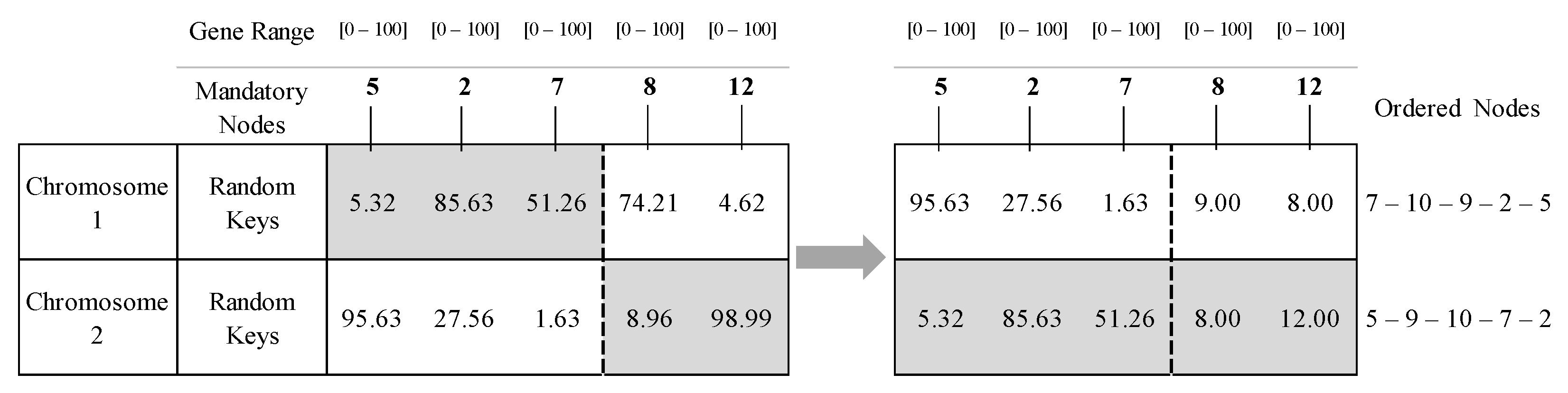
3.3. Global Solution (Global Solution Optimization—GSO)

The AROnGA is modified for the generation of candidate solutions and their evaluation, seeking a robust solution. Every time a candidate solution, Z, is produced, its performance is calculated based on each scenario’s conditions and then compared to the scenario’s benchmark. We obtain the difference as follows:

$${\mathit{dTOT}}_{\mathit{TW},Z}={\mathit{TOT}}_{\mathit{TW},Z}-{{\mathit{TOT}}_{\mathit{TW}}}^{\mathit{min}}$$

(4)

The mean, μ(dTOT_TW,Z), of all said differences is calculated. The AROnGA target is to minimize this mean value:

GSO target: Minimize μ(dTOT_TW,Z)

(5)

The global solution, X*_Z, is then described as follows:

$${X^{\ast }}_Z=\left\{\mu \right({\mathit{TOT}}_{\mathit{TW},Z}), { L}_k, \widehat{S_v^M}\}$$

(6)

4. Application and Results

We tested our proposed framework and methodology on a devised case study.

4.1. Case Study Setup

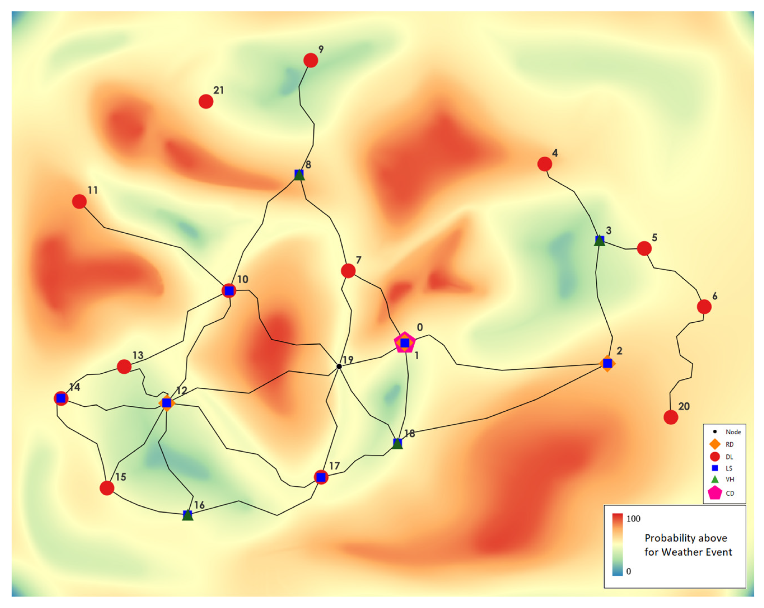
4.1.1. Network

An artificial network, sized like a large city (approximately 50 km × 70 km), was created, along with infrastructure and demand information. The setup contained a mix of features to allow us to test our proposed framework and solution methodology.

4.1.2. Stochastic Traffic Conditions

For each CVN link, a historical database of observed mean CV travel speed, expressed through a normal distribution with a different mean and standard deviation, is assumed. The probability density function for each link’s travel speed can be expressed as follows:

$${P\left(x\right)}_{ij}={\displaystyle \frac{1}{\sigma \sqrt{2\pi }}}{e}^{-{\displaystyle \frac{1}{2}}{\left({\displaystyle \frac{x-\mu }{\sigma }}\right)}^2}$$

(7)

where $\mu$ and ${\sigma }^2$ Are the mean and variance for the variate $x={\mathrm{S}}_{\mathrm{i}\mathrm{j}}^{\mathrm{C}\mathrm{V}}$.

At a selected confidence level, α_Τ = 90%, a total of 30 seeds (“T”) are created, every time assigning a generated mean CV travel speed ($S_{ij,T}^{CV}$) and the resulting travel time (${ct}_{ij,T}$) to each CVN link.

4.1.3. Stochastic Weather Forecast

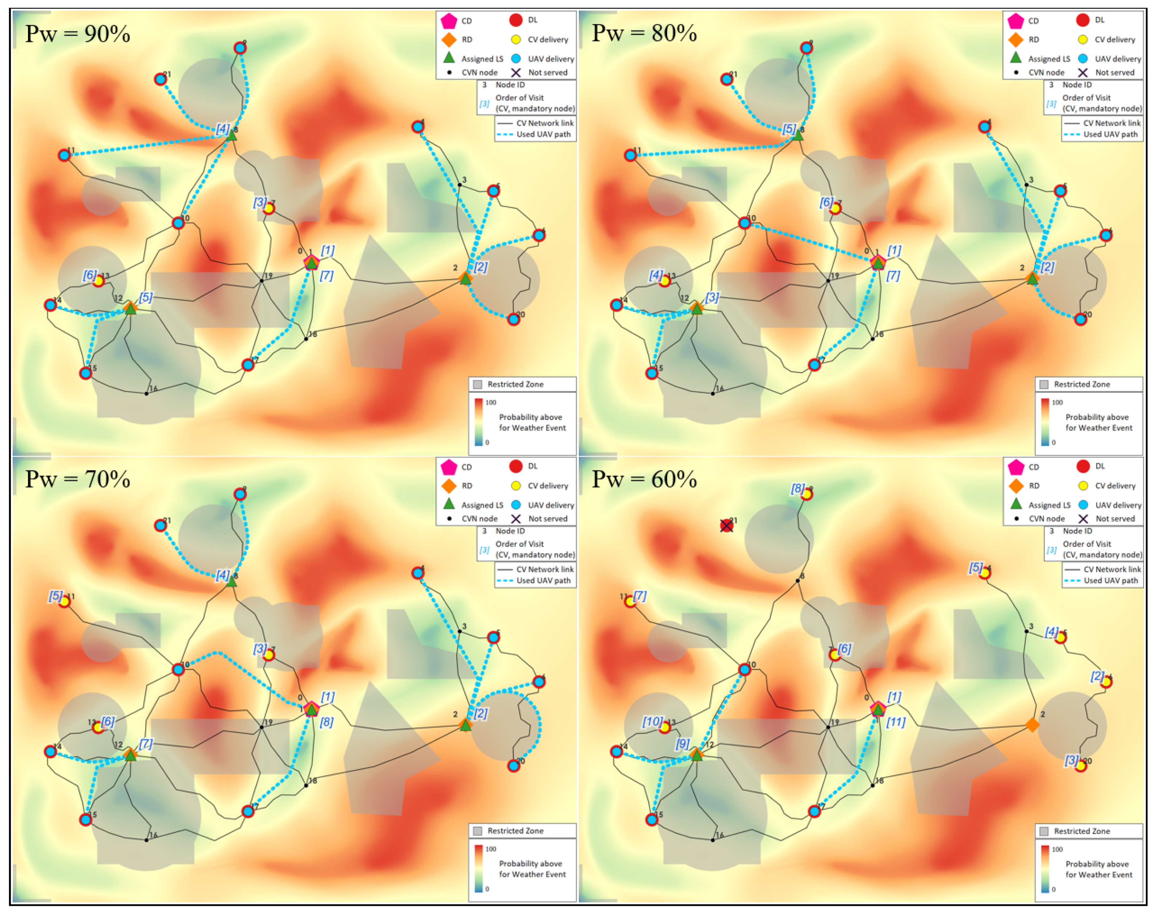
We assume a weather forecast map like that in Figure 1, where areas are characterized based on the probability of falling below or above a certain weather metric. However, since we are specifically interested in adverse conditions for UAV flights, the map contains only information regarding the exceedance of the specified metric. We generate a random probabilistic forecast map and convert said information into a DEM-like feature in GIS; “Pw” values are translated into altitude or “cost”. Figure 5 illustrates the probabilistic weather forecast. Also, the designated locations of the central depot (CD), remote depots (RDs), virtual hubs (VHs), delivery locations (DLs), and launch sites (LSs) are shown.

Performing spatial analysis in GIS, we have further isolated the areas above certain probability thresholds, namely 60%, 70%, 80%, and 90%. Figure 6 shows the threshold-based spatial analysis.

4.2. Experiments

We apply our methodology considering the four probability thresholds of 60, 70, 80, and 90% and the 30 seeds of CVN conditions generated. Initial feasible DL–LS UAV connections are found, based on the theoretical maximum UAV range, with straight paths. RZs and AWZs are considered obstacles for UAV routing. For each Pw scenario, we recalculate the optimal UAV paths for the above LS–DL pairs, using the obstacle avoidance optimal line tools provided in the GIS software packages (Esri ArcGIS Pro 2.8).

Additional constraints in air travel are introduced via no-fly zones, or Restricted zones (RZs). The RZs devised in terms of shape and size are inspired by usual provisions met in real-life cases, like airports, military zones, etc. For each weather risk scenario, the RZs are also combined to produce the final no-fly zones, which are considered as “obstacles” for the UAVs.

A flow direction algorithm [29] is employed for the calculation of shortest paths around the forbidden areas, both for fixed no-fly zones and adverse weather. Figure 7 shows the respective calculated UAV paths for each scenario.

Total flight times, tft_ij,W, are updated based on the new flight paths, and feasible UAV connectivity for each one is reevaluated based on UAV range. The service node pool (SNk) for each DL is produced.

For every scenario, SC_TW, the respective seed’s CV link travel times, ct_ij,T, are used for all relative calculations. Sub-paths between nodes are calculated using the A* algorithm [24]. By implementing the AROnGA, a benchmark solution for each scenario is obtained (

Table 1. Benchmark solution TOT for each scenario.

Seed	TOTTWmin (s)
No	Pw = 90%	Pw = 80%	Pw = 70%	Pw = 60%
1	17,254.37	17,357.06	19,313.74	30,026.49
2	17,037.6	17,080.29	19,140.06	31,269.8
3	17,304.48	17,107.17	17,898.02	32,118.2
4	17,183.86	17,424.87	18,850.66	34,445.35
5	17,091.02	17,267.28	18,094.89	31,162.95
6	17,051.6	17,154.29	19,041.81	32,444.25
7	16,967.73	17,010.42	17,817.36	32,888.2
8	16,929.83	17,032.52	18,068.75	31,419.5
9	17,050.81	17,265.72	18,392.34	30,918.41
10	17,111.56	17,154.25	17,941.08	32,869.8
11	17,117.87	18,572.03	18,078.14	31,771.98
12	17,396.54	17,458.39	18,713.29	31,408.95
13	17,331.62	17,912.38	18,089.26	32,704.41
14	16,813.96	16,856.65	17,575.38	32,269.08
15	16,836.18	16,998.86	17,675.42	32,363.35
16	17,297.96	17,661.77	18,808.39	32,273.38
17	16,982.43	17,223.15	17,891.34	33,134.36
18	17,134.69	17,237.38	18,024.82	31,774.46
19	16,910.51	17,256.32	18,232.15	31,178.88
20	17,592.35	17,635.04	18,374.9	33,814.77
21	17,178.89	17,281.58	18,013.08	31,477.1
22	17,192.75	17,454.72	19,359.49	34,143.58
23	17,118.12	17,111.2	18,009.42	32,080.94
24	16,839.37	16,942.06	18,012.9	32,377.86
25	17,226.31	17,089	18,752.7	31,549.68
26	16,986.16	17,200.96	17,928.83	32,702.52
27	17,473.45	17,516.14	18,069.77	30,442.2
28	17,271.92	17,330.34	18,093.73	32,777.06
29	17,288.01	18,362.71	18,763.22	33,741.98
30	17,064.99	17,107.68	17,979.79	31,751.01

).

The above benchmarks are used for obtaining a global solution for each weather forecast confidence threshold.

Table 2. Global Solutions for each scenario.

Item (k)	Node (dk)	Service Node Pool [SNk]	Service Node (lk)	Mode	Service Node Pool [SNk]	Service Node (lk)	Mode
		Pw = 90%			Pw = 80%
1	4	[‘4’, ‘0’, ‘1’, ‘2’, ‘3’]	2	UAV	[‘4’, ‘2’, ‘3’]	2	UAV
2	5	[‘5’, ‘2’, ‘3’]	2	UAV	[‘5’, ‘2’, ‘3’]	2	UAV
3	6	[‘6’, ‘2’, ‘3’]	2	UAV	[‘6’, ‘2’, ‘3’]	2	UAV
4	7	[‘7’]	7	CV	[‘7’]	7	CV
5	9	[‘9’, ‘8’]	8	UAV	[‘9’, ‘8’]	8	UAV
6	10	[‘10’, ‘0’, ‘1’, ‘8’, ‘12’, ‘14’]	8	UAV	[‘10’, ‘0’, ‘1’, ‘8’, ‘12’, ‘14’]	0	UAV
7	11	[‘11’, ‘8’, ‘10’, ‘14’]	8	UAV	[‘11’, ‘8’, ‘10’, ‘14’]	8	UAV
8	13	[‘13’]	13	CV	[‘13’]	13	CV
9	14	[‘14’, ‘10’, ‘12’]	12	UAV	[‘14’, ‘10’, ‘12’]	12	UAV
10	15	[‘15’, ‘12’, ‘14’]	12	UAV	[‘15’, ‘12’, ‘14’]	12	UAV
11	17	[‘17’, ‘0’, ‘1’, ‘18’]	0	UAV	[‘17’, ‘0’, ‘1’, ‘18’]	0	UAV
12	20	[‘20’, ‘2’, ‘3’]	2	UAV	[‘20’, ‘2’, ‘3’]	2	UAV
13	21	[‘8’, ‘10’]	8	UAV	[‘8’, ‘10’]	8	UAV
$T_M^v$		[‘0’, ‘2’, ‘7’, ‘8’, ‘12’, ‘13’]			[‘0’, ‘2’, ‘7’, ‘8’, ‘12’, ‘13’]
$\widehat{S_v^M}$		[‘0’, ‘2’, ‘7’, ‘8’, ‘12’, ‘13’, ‘1’]			[‘0’, ‘2’, ‘12’, ‘13’, ‘8’, ‘7’, ‘1’]
$\widehat{S_{\left(e\right)}^M}$		[(‘0’, ‘2’), (‘2’, ‘7’), (‘7’, ‘8’), (‘8’, ‘12’), (‘12’, ‘13’), (‘13’, ‘1’)]			[(‘0’, ‘2’), (‘2’, ‘12’), (‘12’, ‘13’), (‘13’, ‘8’), (‘8’, ‘7’), (‘7’, ‘1’)]
Mean dTOT		332.7 s/5.5 min			168.2 s/2.8 min
$\mathrm{Mean} {{\mathrm{TOT}}_{\mathrm{TW}}}^{\min }$		17,134.6 s/285.6 min			17,335.4 s/288.9 min
$\mathrm{Min}/\mathrm{Max} {{\mathrm{TOT}}_{\mathrm{TW}}}^{\min }$		280.2/293.2 min			280.9/309.5 min
		Pw = 70%			Pw = 60%
1	4	[‘4’, ‘2’, ‘3’]	2	UAV	[‘4’]	4	CV
2	5	[‘5’, ‘2’, ‘3’]	2	UAV	[‘5’, ‘3’]	5	CV
3	6	[‘6’, ‘2’, ‘3’]	2	UAV	[‘6’, ‘3’]	6	CV
4	7	[‘7’]	7	CV	[‘7’]	7	CV
5	9	[‘9’, ‘8’]	8	UAV	[‘9’]	9	CV
6	10	[‘10’, ‘0’, ‘1’, ‘8’, ‘12’, ‘14’]	0	UAV	[‘10’, ‘12’, ‘14’]	12	UAV
7	11	[‘11’]	11	UAV	[‘11’]	11	CV
8	13	[‘13’]	13	CV	[‘13’]	13	CV
9	14	[‘14’, ‘10’, ‘12’]	12	UAV	[‘14’, ‘10’, ‘12’]	12	UAV
10	15	[‘15’, ‘12’, ‘14’]	12	UAV	[‘15’, ‘12’, ‘14’]	12	UAV
11	17	[‘17’, ‘0’, ‘1’, ‘18’]	0	UAV	[‘17’, ‘0’, ‘1’, ‘18’]	0	UAV
12	20	[‘20’, ‘2’]	2	UAV	[‘20’]	20	CV
13	21	[‘8’]	8	UAV	[(no service)]	n/a	n/a
$T_M^v$		[‘0’, ‘2’, ‘7’, ‘8’, ‘11’, ‘12’, ‘13’]			[‘0’, ‘4’, ‘5’, ‘6’, ‘7’, ‘9’, ‘11’, ‘12’, ‘13’, ‘20’]
$\widehat{S_v^M}$		[‘0’, ‘2’, ‘7’, ‘8’, ‘11’, ‘13’, ‘12’, ‘1’]			[‘0’, ‘6’, ‘20’, ‘5’, ‘4’, ‘7’, ‘11’, ‘9’, ‘12’, ‘13’, ‘1’]
$\widehat{S_{\left(e\right)}^M}$		[(‘0’, ‘2’), (‘2’, ‘7’), (‘7’, ‘8’), (‘8’, ‘11’), (‘11’, ‘13’), (‘13’, ‘12’), (‘12’, ‘1’)]			[(‘0’, ‘6’), (‘6’, ‘20’), (‘20’, ‘5’), (‘5’, ‘4’), (‘4’, ‘7’), (‘7’, ‘11’), (‘11’, ‘9’), (‘9’, ‘12’), (‘12’, ‘13’), (‘13’, ‘1’)]
Mean dTOT		264.1 s/4.4 min			754.4 s/12.6 min
$\mathrm{Mean} {{\mathrm{TOT}}_{\mathrm{TW}}}^{\min }$		18,300.2 s/305.0 min			32,176.7 s/536.3 min
$\mathrm{Min}/\mathrm{Max} {{\mathrm{TOT}}_{\mathrm{TW}}}^{\min }$		292.9/322.7 min			500.4/574.1 min

shows the results of the GSO for each weather forecast scenario.

Figure 8 illustrates the solutions by highlighting the mandatory nodes and their order of visit, as well as the UAV connections used for item delivery.

We now interpret the practical implications of the above results. For example, for the case of Pw = 90%, the average expected operations time would be 285.6 min (minimum: 280.2 min; maximum: 293.2 min). If the assignment and basic routing proposal are followed, no matter the conditions on the road, the performance of planned operations will be, on average, 5.5 min slower than the theoretical best for the conditions met, that is, 1.94% off the average value among generated seeds. This is essentially the average time the planner should be prepared to “sacrifice” for a more reliable and satisfactory result in operational performance. For the case of Pw = 80%, only an extra 2.8 min (or 0.97% of the average expected TOT_TW^min = 288.9 min) is sacrificed to achieve robust performance. It is also evident that as confidence in the weather forecast decreases, more items are assigned to CVs because of fewer UAV connections and longer flight times. Sometimes a counterintuitive solution may appear; however, we should bear in mind that this is intended to tackle any conditions met on the network and not just a specific case.

5. Conclusions

We have developed a solution methodology for strategic planning under uncertainty, using a scenario-based robust optimization process and a tailored assignment and routing optimization nested genetic algorithm. The methodology yields optimal solutions for given conditions concerning the CVN and the airspace and then provides a robust solution that performs well under a variety of circumstances. It offers the option of selecting the level of risk a planner is willing to take (in terms of CVN conditions and the weather) and proposes how the items should be delivered and what route the CV should follow to avoid excess delays. The methodology does not provide a total route for the CV but highlights the mandatory nodes and the order of visit for prior planning. If the conditions are given, the methodology can also propose an exact path for the CV. Additionally, it is reasonable to expect that a larger, more complex network would offer more alternatives in assignment and routing, and the global solution would fare, on average, worse than the theoretical best for each generated scenario.

References

1. ITF. Ready for Take Off? Integrating Drones into the Transport System; OECD Publishing: Paris, France, 2021. [Google Scholar]
2. Davies, C. The Carbon Cost of Home Delivery and How to Avoid It. Horizon: The EU Research & Innovation Magazine, 17 February 2020. [Google Scholar]
3. ICAO. Annex 2 to the Convention on Civil Aviation—Rules of the Air, 10th ed.; International Civil Aviation Organization: Montreal, QC, Canada, 2005. [Google Scholar]
4. Murray, C.C.; Chu, A.G. The Flying Sidekick Traveling Salesman Problem: Optimization of Drone-Assisted Parcel Delivery. Transp. Res. Part C Emerg. Technol. 2015, 54, 86–109. [Google Scholar] [CrossRef]
5. Moshref-Javadi, M.; Lee, S.; Winkenbach, M. Design and Evaluation of a Multi-Trip Delivery Model with Truck and Drones. Transp. Res. Part E Logist. Transp. Rev. 2020, 136, 101932. [Google Scholar] [CrossRef]
6. Salama, M.R.; Srinivas, S. Collaborative Truck Multi-Drone Routing and Scheduling Problem: Package Delivery with Flexible Launch and Recovery Sites. Transp. Res. Part E Logist. Transp. Rev. 2022, 164, 102788. [Google Scholar] [CrossRef]
7. Marinelli, M.; Caggiani, L.; Ottomanelli, M.; Dell’Orco, M. En Route Truck–Drone Parcel Delivery for Optimal Vehicle Routing Strategies. IET Intell. Transp. Syst. 2017, 12, 295–302. [Google Scholar] [CrossRef]
8. Macrina, G.; Di Pugliese, L.; Guerriero, F.; Laporte, G. Drone-Aided Routing: A Literature Review. Transp. Res. Part C Emerg. Technol. 2020, 120, 102762. [Google Scholar] [CrossRef]
9. Gendreau, M.; Laporte, G.; Séguin, R. Stochastic Vehicle Routing. Eur. J. Oper. Res. 1996, 88, 3–12. [Google Scholar] [CrossRef]
10. Bertsimas, D.J.; Simchi-Levi, D. A New Generation of Vehicle Routing Research: Robust Algorithms Addressing Uncertainty. Oper. Res. 1996, 44, 286–304. [Google Scholar] [CrossRef]
11. Wu, L.; Hifi, M. Discrete Scenario-Based Optimization for the Robust Vehicle Routing Problem: The Case of Time Windows under Delay Uncertainty. Comput. Ind. Eng. 2020, 145, 106491. [Google Scholar] [CrossRef]
12. Kepaptsoglou, K.; Fountas, G.; Karlaftis, M.G. Weather Impact on Containership Routing in Closed Seas: A Chance-Constraint Optimization Approach. Transp. Res. Part C Emerg. Technol. 2015, 55, 139–155. [Google Scholar] [CrossRef]
13. Zhan, W.; Wang, W.; Chen, N.; Wang, C. Efficient UAV Path Planning with Multiconstraints in a 3D Large Battlefield Environment. Math. Probl. Eng. 2014, 2014, 597092. [Google Scholar] [CrossRef]
14. Zhang, M.; Su, C.; Liu, Y.; Hu, M.; Zhu, Y. Unmanned Aerial Vehicle Route Planning in the Presence of a Threat Environment Based on a Virtual Globe Platform. ISPRS Int. J. Geo-Inf. 2016, 5, 192. [Google Scholar] [CrossRef]
15. Zhang, Y.; Li, X.; Wang, J.; Liu, Y. Truck-Drone Delivery Optimization Based on Multi-Agent Reinforcement Learning. Drones 2024, 8, 27. [Google Scholar] [CrossRef]
16. Jeong, H.; Lee, D. Drone Routing Problem with Truck: Optimization and Quantitative Analysis. Expert Syst. Appl. 2023, 227, 120260. [Google Scholar] [CrossRef]
17. Wang, S.; Zhao, Y. Optimal Delivery Route Planning for a Fleet of Heterogeneous Drones: A Rescheduling-Based Genetic Algorithm Approach. Comput. Ind. Eng. 2023, 179, 109179. [Google Scholar] [CrossRef]
18. Joo, J.; Lee, C. A Branch-and-Price Algorithm for Robust Drone-Vehicle Routing Problem with Time Windows. Inf. J. Comput. 2025, 37, 1–15. [Google Scholar] [CrossRef]
19. Tolooie, A.; Sinha, A.; Khosh Raftar Nouri, A. Heuristic Approach for Optimizing Reliable Supply Chain Network Using Drones in Last-Mile Delivery under Uncertainty. Int. J. Syst. Sci. Oper. Logist. 2024, 11, 2301610. [Google Scholar]
20. Deng, M.; Li, Y.; Ding, J.; Zhou, Y.; Zhang, L. Stochastic and Robust Truck-and-Drone Routing Problems with Deadlines: A Benders Decomposition Approach. Transp. Res. Part E Logist. Transp. Rev. 2024, 190, 103709. [Google Scholar] [CrossRef]
21. Wei, S.; Fan, H.; Ren, X.; Diao, X. Time-Dependent Vehicle Routing Problem with Drones under Vehicle-Restricted Zones and No-Fly Zones. Appl. Sci. 2025, 15, 2207. [Google Scholar] [CrossRef]
22. Mahmoodi, A.; Sajadi, S.M.; Sadeq, A.M.; Narenji, M.; Eshaghi, M.; Jasemi, M. Enhancing Unmanned Aerial Vehicles Logistics for Dynamic Delivery: A Hybrid Non-Dominated Sorting Genetic Algorithm II with Bayesian Belief Networks. Ann. Oper. Res. 2025, 325, 123–145. [Google Scholar] [CrossRef]
23. Zhang, Y.; Wang, L.; Liu, Q.; Chen, H. Exact Solution of the Vehicle Routing Problem with Drones. Transp. Sci. 2024, 58, 345–362. [Google Scholar]
24. Wang, W.; Zhang, M.; Beech, E.; Majumdar, A.; Ochieng, W.; Escribano, J. Risk-Based Truck-Drone Delivery Optimization. In Proceedings of the TRISTAN XII: Triennial Symposium on Transportation Analysis, Okinawa, Japan, 22–27 June 2025; pp. 163–170. [Google Scholar]
25. Gonzalez-R, P.L.; Canca, D.; Andrade-Pineda, J.L.; Calle, M.; Leon-Blanco, J.M. Truck-Drone Team Logistics: A Heuristic Approach to Multi-Drop Route Planning. Transp. Res. Part C Emerg. Technol. 2020, 114, 657–680. [Google Scholar] [CrossRef]
26. Doswell, C.; Brooks, H. NOAA National Severe Storms Laboratory. Available online: https://www.nssl.noaa.gov/users/brooks/public_html/prob/Probability.html (accessed on 21 March 2023).
27. World Climate Service. WCS Blog—Analysis from the World Climate Service. Available online: https://www.worldclimateservice.com/2021/09/08/probability-forecast/ (accessed on 21 March 2023).
28. Kouretas, K.; Kepaptsoglou, K. Planning Integrated Unmanned Aerial Vehicle and Conventional Vehicle Delivery Operations under Restricted Airspace: A Mixed Nested Genetic Algorithm and Geographic Information System-Assisted Optimization Approach. Vehicles 2023, 5, 1060–1086. [Google Scholar] [CrossRef]
29. ESRI. Flow Direction. Available online: https://desktop.arcgis.com/en/arcmap/latest/tools/spatial-analyst-toolbox/flow-direction.htm (accessed on 25 June 2023).
Figure 1. WCS surface temperature probability map with a week 2 lead time; source: [26].
Drones 09 00359 g001
Figure 2. General workflow.
Drones 09 00359 g002
Figure 3. Outer GA example (mode assignment).
Drones 09 00359 g003
Figure 4. Inner GA example (routing).
Drones 09 00359 g004
Figure 5. Introduced probabilistic weather forecast.
Drones 09 00359 g005
Figure 6. Spatial analysis based on probability thresholds.
Drones 09 00359 g006
Figure 7. Optimal UAV flight paths for feasible DL–LS pairs per weather forecast scenario.
Drones 09 00359 g007
Figure 8. Illustration of the estimated global solution by weather forecast scenario.
Drones 09 00359 g008