Safe and Optimal Motion Planning for Autonomous Underwater Vehicles: A Robust Model Predictive Control Framework Integrating Fast Marching Time Objectives and Adaptive Control Barrier Functions

Abstract

Autonomous Underwater Vehicles (AUVs) have shown significant promise across various underwater applications, yet face challenges in dynamic environments due to the limitations of traditional motion planning methods while Artificial Potential Field (APF)-based control barrier functions focus solely on obstacle proximity and distance-based methods oversimplify obstacle geometries, and both fail to ensure safety and satisfy turning radius constraints for under-actuated AUVs in intricate environments. This paper proposes a robust Model Predictive Control (MPC) framework integrating an enhanced fast marching control barrier function, specifically designed for AUVs equipped with fully directional sonar systems. The framework introduces a novel improvement for moving obstacles by extending the control barrier function field propagation along the obstacle’s movement direction. This enhancement generates precise motion plans that ensure safety, satisfy kinematic constraints, and effectively handle static and dynamic obstacles. Simulation results demonstrate superior obstacle avoidance and motion planning performance in complex scenarios, with key outcomes including a minimum safety margin of 1.86 m in cluttered environments (vs. 0 m for A* and FMM) and 1.76 m in dynamic obstacle scenarios (vs. 0.13 m for MPC-APFCBF), highlighting the framework’s ability to enhance navigation safety and efficiency for real-world AUV deployments in unpredictable marine environments.

1. Introduction

Autonomous Underwater Vehicles (AUVs) excel in underwater operations such as seabed mapping and pipeline inspection due to their superior maneuverability [1]. Their motion planning systems enable autonomous navigation by generating collision-free trajectories through complex marine environments. Integrated high-precision INS [2] with multi-sensor fusion provides real-time navigation data and precise obstacle localization, allowing accurate calculation of safety distances and boundary constraints. This integration ensures reliable obstacle avoidance and safe path planning for AUVs operating in challenging underwater conditions.

AUV motion planning research focuses on global and local techniques [3]. Global methods, adapted from terrestrial robotics, include graph search algorithms (Dijkstra’s [4], A* [5], D*), sampling-based approaches (RRT, PRM [6]), optimization algorithms (genetic algorithms, simulated annealing, particle swarm optimization [7]), and heuristic methods (ant colony algorithms [8]). These have been modified for marine applications. Intelligent techniques like neural networks [9], deep learning [10], and reinforcement learning [11] are also utilized. The study in reference [12] introduced an Integral Reinforcement Learning (IRL)-based global planning approach that achieves optimized motion planning through online learning and iterative updates. However, the complexity of marine environments often limits global methods to providing only initial reference trajectories, as they struggle with real-time re-planning demands.

To tackle the issue of rapid online planning, several local motion planning methods have been put forward. These include artificial potential field methods [13], the dynamic window approach [14], and fuzzy logic control [15]. Because Model Predictive Control (MPC) can conduct online rolling optimization, it finds widespread application in the motion planning of marine vehicles. Recent advancements in MPC-based planning for autonomous marine vehicles were systematically reviewed in reference [16], highlighting its adaptability in hydrodynamic environments. However, critical gaps persist, particularly in ensuring operational safety under complex constraints, including real-time collision avoidance guarantees and formal safety verification mechanisms for dynamic obstacle scenarios.

In reference [17], spline functions were introduced as templates for the path planning of AUVs by MPC. Simulation experiments verified the feasibility of their MPC-based dynamic path planning algorithm. Subsequently, in reference [18], taking advantage of MPC’s remarkable real-time optimization capabilities, a receding horizon optimization (RHO) scheme was put forward, which exhibited strong stability and effectiveness during path planning. Reference [19] incorporated the arrival time matrix derived from the fast marching method into the MPC objective function. By doing so, it managed to reduce the path-traversing time within short prediction horizons. The authors in reference [20] developed an integrated perception-planning framework, where sonar-based environmental imaging was processed through convolutional neural networks (CNNs) and Transformers for precise obstacle detection and characterization. This perceptual data was subsequently integrated with MPC for real-time collision avoidance. In the research domain of AUV path planning and control, Shen et al. developed a tracking control algorithm that was integrated with dynamic path planning [18].

The synergistic integration of MPC with Control Barrier Functions (CBFs) represents a transformative approach to safety-critical motion planning, ensuring real-time constraint satisfaction while maintaining system agility. There are two types of control barrier functions, namely the zeroing and reciprocal barrier functions, which are designed to ensure that the system state remains within a safe set [21]. In recent years, these functions have witnessed widespread utilization in the realm of robot safety motion planning. In reference [22], discrete-time CBFs grounded in MPC control are introduced to handle external position disturbances. Additionally, moving horizon estimation (MHE) is employed to approximate the truncation errors that arise from the discretion process. Reference [23] also makes use of discrete control barrier functions, integrating them with a model predictive control framework to realize safety-critical motion planning for robots. Reference [24] establishes an elliptical equation for obstacles to calculate the distances and construct CBFs for obstacle avoidance. Nonetheless, references [22,23,24] abstracts obstacles into circular or spherical shapes. This approach suffers from a lack of adaptability to various other shapes. In response to this limitation, reference [25] proposes an obstacle avoidance barrier function tailored for polyhedral obstacles in robots’ environments. By combining it with MPC, safety-critical motion planning can be achieved. Reference [26] indicates that non-smooth control barrier functions can be applied to motion planning. However, both references [25,26] concentrate on regular rectangular or polyhedral obstacles.

In reference [27], a comparison is made between control barrier functions and artificial potential fields in the context of robot motion planning, which is called model predictive control—artificial potential field control barrier function (MPC-APFCBF) in this paper. Corresponding control barrier functions are designed based on the attraction and repulsion functions of artificial potential fields. In reference [28], a novel approach is proposed to enhance Unmanned Aerial Vehicle (UAV) safety through the establishment of extended interference dead zones specifically designed for unknown and moving obstacles. Reference [29] also focuses on dynamic obstacle environments, proposing a perception-aware online trajectory generation system for Unmanned Surface Vehicles (USVs) to perform prescribed maneuvers in dynamic unstructured environments. This system combines the Inverse Dynamics in the Virtual Domain (IDVD) method with an Event-Triggered Receding Horizon Control (ETRHC) mechanism, enabling the generation of safe and quasi-optimal trajectories in real-time. The effectiveness and robustness of the approach were validated through simulations. Reference [30] presents a composite strategy that integrates an enhanced A* algorithm with MPC to improve path planning and dynamic obstacle avoidance for UUVs in complex marine environments, where obstacles are modeled as spheres and cylinders.

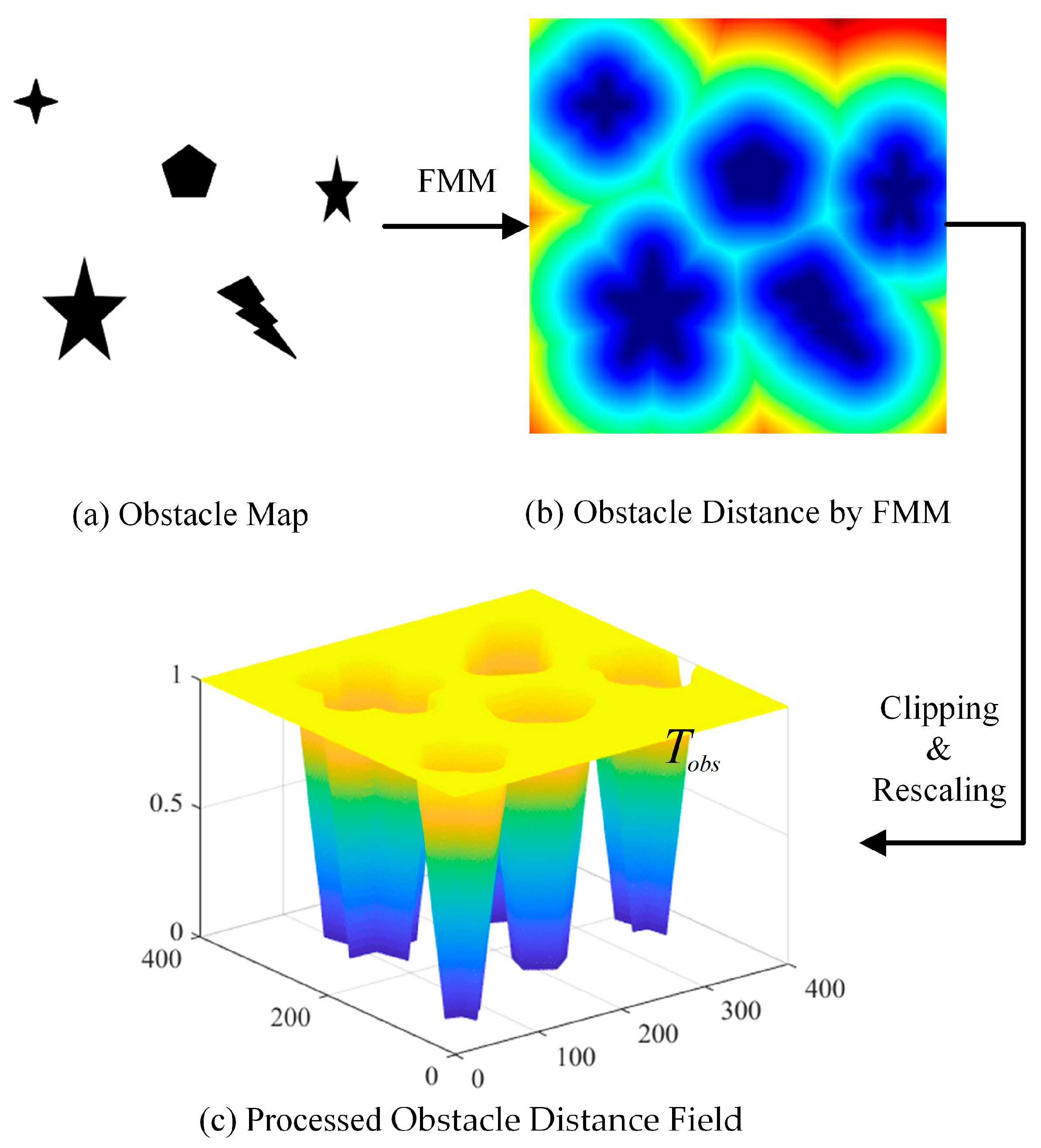
In general, the fundamental principle of combining MPC with CBFs is as follows: MPC generates trajectories through rolling horizon optimization, making it well-suited for real-time motion planning. CBFs ensure system safety by constructing a safety function as a constraint within the MPC framework, guaranteeing that the system state remains within a predefined safe set. However, existing studies still face significant challenges in ensuring safety in environments with narrow or irregularly shaped obstacles, as well as in scenarios involving dynamic or moving obstacles. In practice, AUVs operate in underwater environments that are often cluttered with obstacles of varying shapes and narrow passageways, where safety is paramount. To bridge the gap between current research and real-world requirements, this paper proposes an obstacle avoidance barrier function based on a fast marching algorithm, specifically designed to address these challenges. In summary, the innovations of this paper can be summarized as follows:

(1) Novel FMM-based CBF for Complex Obstacle Geometries: A new control barrier function based on the fast marching algorithm (FMM) is proposed, specifically designed to handle environments with complex and intricate obstacle shapes. This approach overcomes the limitations of traditional methods that rely on simplified obstacle representations (e.g., circles or polygons).

(2) Dynamic Obstacle Handling via Velocity-Adjusted FMM Propagation: An enhanced method for dynamic obstacle avoidance is introduced, which extends the control barrier function field propagation along the direction of obstacle movement. This ensures that the AUV maintains a safe clearance from moving obstacles, even in highly dynamic environments.

(3) Robust MPC-FMCBF Framework Validated in Simulations: A robust MPC framework is developed, integrating the proposed fast marching-based control barrier function (FMCBF). This framework effectively ensures AUV safety in complex environments while significantly improving navigation security, as demonstrated through extensive simulations.

The remainder of this paper is structured as follows: Section 2 presents the problem description. Section 3 provides the model of AUV. Section 4 details the proposed algorithm, which is analyzed in Section 5. Simulation results are presented in Section 6. Finally, Section 7 concludes the paper.

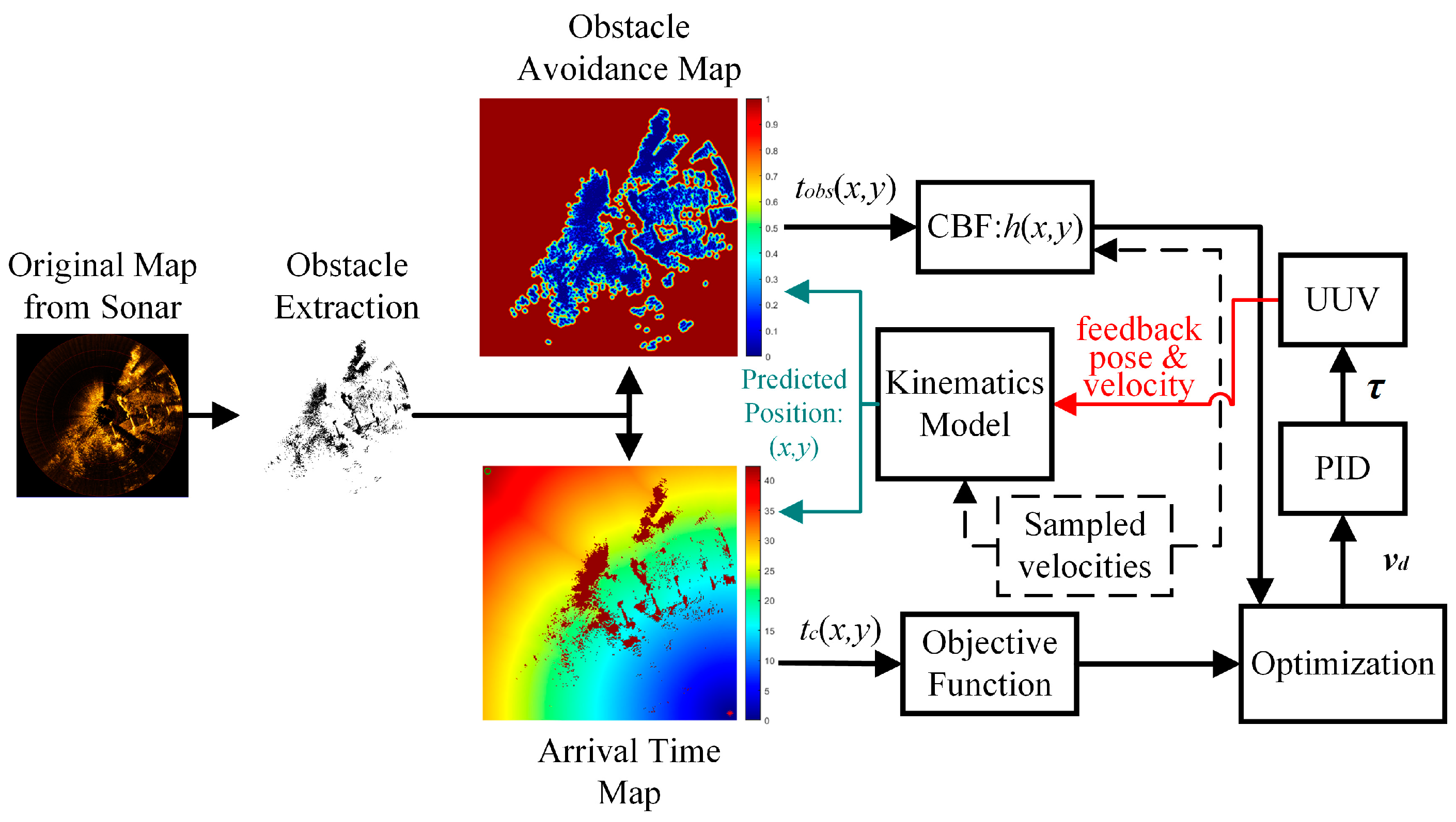
2. Problem Description

Research in underwater vehicle motion planning primarily concentrates on the generation of optimal linear and angular velocity profiles for AUVs to ensure safe and efficient navigation from initial to target positions in obstacle-rich environments. Following deployment and descent to operational depth, AUVs typically execute critical missions including seabed mapping, environmental monitoring, and target detection. Consequently, this study focuses on two-dimensional (2D) motion planning for AUV operations at fixed depth. The primary objectives of motion planning encompass the following: (1) minimization of navigation cost metrics (including but not limited to travel distance, time efficiency, and energy expenditure), (2) adherence to the vehicle’s kinematic constraints, and (3) guaranteed collision avoidance. Based on these considerations, the motion planning problem can be formally modeled as follows:

$$\begin{array}{l}\underset{{\mathit{v}}_1,{\mathit{v}}_2,\dots ,{\mathit{v}}_n}{\mathrm{argmin}}J\\ \begin{array}{cc}s.t.& {\dot{\mathit{\eta }}}_i\end{array}=f({\mathit{\eta }}_{i-1},{\mathit{v}}_{i-1}),i=2,\dots ,n+1\\ {\mathit{v}}_i\in {\mathrm{S}}_{\mathit{v}},i=1,2,\dots ,n\\ {\mathit{\eta }}_1={\mathit{\eta }}_{start},{\mathit{\eta }}_{n+1}\in \mathrm{U}({\mathit{\eta }}_{goal},\mathsf{\epsilon })\\ {\mathit{\eta }}_i\cap \left\{O\right\}=\varnothing ,i=1,\dots ,n+1\end{array}$$

(1)

In this study, vector and matrix quantities are denoted using boldface notation. The kinematic constraints of the AUV are represented by ${\dot{\mathit{\eta }}}_i=f({\mathit{\eta }}_{i-1},{\mathit{v}}_{i-1})$. To ensure computational efficiency for real-time implementation, the motion planning framework incorporates only the kinematic model of the AUV. The primary objective of the motion planning algorithm is to compute an optimal velocity profile within the range $S_{\mathit{v}}$, enabling the AUV to navigate from its initial position ${\mathit{\eta }}_{start}$ to a predefined target ${\mathit{\eta }}_{goal}$ neighborhood $\mathsf{\epsilon }$. This optimization process simultaneously minimizes the specified objective function while guaranteeing collision-free trajectories through obstacle-rich environments.

3. Model of Autonomous Underwater Vehicle

3.1. Kinematics Model

This paper simplifies motion planning in 2D environments. As is shown in Figure 1, the earth-fixed (O-xy) frame in black arrows and body-fixed (o-xy) frame in red arrows are established. The coordinate transform is as Equations (2) and (3).

$$\dot{\mathit{\eta }}=J(\psi )\mathit{v}=f(\mathit{\eta },\mathit{v})$$

(2)

$$\mathit{J}(\psi )=\left[\begin{array}{ccc}\cos \psi & -\sin \psi & 0\\ \sin \psi & \cos \psi & 0\\ 0& 0& 1\end{array}\right]$$

(3)

In (2), $\mathit{\eta }={[x,y,\psi ]}^{\mathrm{T}}$ contains the position coordinates and the yaw angle in radians in the 2D earth-fixed frame, and $\mathit{v}={[u,0,r]}^{\mathrm{T}}$ is the absolute velocity vector in the body-fixed frame.

3.2. Dynamics Model

According to the balance of forces and moments, the dynamics model of AUV [31] can be expressed by Equation (4).

$$\left[\begin{array}{ccc}m-X_{\dot{u}}& 0& 0\\ 0& m& 0\\ 0& 0& I_z-N_{\dot{r}}\end{array}\right]\dot{\mathit{v}}+\left[\begin{array}{ccc}-X_u-X_{u\left|u\right|}\left|u\right|& 0& 0\\ 0& 0& (m-X_{\dot{u}})u\\ 0& 0& -N_r-N_{r\left|r\right|}\left|r\right|\end{array}\right]\mathit{v}=\mathit{\tau }$$

(4)

In Equation (4), $m$ is the mass of the AUV, $I_z$ is its rotational moment of inertia, $X_{\dot{u}}$ and $N_{\dot{r}}$ are the adding masses, $X_u$ and $N_r$ are linear damping coefficients, $X_{u\left|u\right|}$ and $N_{r\left|r\right|}$ are the quadratic damping coefficients, and $\tau ={[F_x,0,T_z]}^{\mathrm{T}}$ contains the forces and moments from the thruster.

It is important to note that the current AUV model in this study does not account for water currents. While water currents are indeed a significant factor in underwater environments, as highlighted in reference [32], they are typically minimal in deeper regions where AUVs often operate. The exclusion of water currents in this work allows us to focus on the core challenges of obstacle avoidance and motion planning in complex environments. This extension will involve incorporating hydrodynamic models to enhance the robustness and applicability of the algorithm in real-world underwater conditions.

In this study, we focus on motion planning in a 2D plane to simplify the problem and demonstrate the core capabilities of the proposed framework. However, the methodology can be extended to 3D environments by adapting the Fast Marching Method to 3D grids and modifying the kinematic models accordingly. While this extension is theoretically feasible, it would significantly increase computational complexity, as the complexity grows quadratically with grid resolution. This could pose challenges for real-time implementation, particularly in large-scale or high-resolution environments. To address this, future work will focus on optimizing the algorithm for 3D applications, potentially leveraging parallel computing techniques or adaptive grid refinement to maintain real-time performance. This extension will enable the framework to handle full 3D motion planning, further enhancing its applicability to real-world AUV operations in complex underwater environments.

4. Proposed Algorithm

AUV motion planning necessitates optimizing objective functions through velocity planning while adhering to system constraints. Given its inherent capability to handle constrained optimization problems, MPC emerges as an ideal solution. This paper presents a robust MPC framework for AUV motion planning, where the MPC generates optimal velocity references for a PID-based velocity tracking controller.

4.1. Integrated Model Predictive Control Framework

The proposed model predictive control framework seamlessly integrates the temporal optimization objective, derived from the arrival time map, with dynamic obstacle avoidance constraints generated through the fast-marching method. This sophisticated integration mechanism empowers the AUV to compute both time-optimal and collision-free trajectories toward its target destination. As depicted in Figure 2, the system architecture implements a multi-stage operational pipeline: Employing state-of-the-art sensing capabilities, the autonomous underwater vehicle initiates its operation by performing comprehensive high-resolution environmental mapping through an advanced sonar system, specifically utilizing the Kongsberg MS1000 sourced from kongsberg maritime, Kongsberg, Norway renowned for its superior acoustic imaging performance. The acquired barometric data undergo advanced processing to construct a detailed environmental representation. Subsequently, the fast-marching algorithm processes this spatial dataset to simultaneously generate two critical navigation components: (1) a temporal arrival map for trajectory optimization and (2) a dynamic obstacle map for safety assurance, both of which serve as fundamental inputs to the MPC’s optimization engine.

$$\begin{array}{l}\underset{{\mathit{v}}_k,\dots ,{\mathit{v}}_{k+c}}{\min }{\displaystyle \sum _{i=k+1}^{k+p-1}Q{t}_c(x_i,y_i)}+Q_p{t}_c(x_{k+p},y_{k+p})+{\displaystyle \sum _{i=k}^{k+c}\mathit{R}{\mathit{v}}_i}\\ s.t.\hspace{1em}{\dot{\mathit{\eta }}}_i=\left\{\begin{array}{c}f({\mathit{\eta }}_{i-1},{\mathit{v}}_{i-1}),i<k+c\\ f({\mathit{\eta }}_{i-1},{\mathit{v}}_{k+c}),\mathrm{else}\end{array}\right.,i=k+1,\dots ,k+p\\ {\mathit{v}}_i\in {\mathrm{S}}_{\mathit{v}},i=k,\dots ,k+c\\ t_c(x_{k+p},y_{k+p})\le t_c(x_k,y_k)\\ h(x_{i+1},y_{i+1})-h(x_i,y_i)\ge -\gamma h(x_i,y_i),i=k+1,\dots ,k+p\end{array}$$

(5)

The model predictive control (MPC) rolling horizon formulation (5) is used to obtain the optimized velocity sequence ${\mathit{v}}_k,\dots ,{\mathit{v}}_{k+c}$, with ${\mathit{v}}_k$ being the desired velocity at time $k$ sent to the AUV’s velocity tracking controller. During motion planning, the AUV’s velocity ${\mathit{v}}_k,\dots ,{\mathit{v}}_{k+c}$ is sampled within the control time domain $c+1$, and the kinematics model predicts the AUV’s pose within the prediction time domain $p$. The first and second constraint functions in Equation (5) represent the kinematic limits of the AUV, ensuring that its motion adheres to the vehicle’s physical capabilities. The third constraint function is designed to prevent the AUV from reversing its direction, maintaining forward progress toward the target. Finally, the last constraint function incorporates the control barrier function, which ensures collision-free navigation by enforcing safety margins around obstacles. The control barrier function $h(x,y)$ is based on the obstacle avoidance map, while the arrival time map $t_c(x,y)$ serves as the objective function to expedite reaching the endpoint.

4.2. Fast Marching-Based Control Barrier Function for Intricate Obstacle Avoidance

Control barrier functions are widely used in robotic safety control problems. For instance, in Equation (6), a closed set $C$ satisfying $h(x)\ge 0$ and $h(x)$ as a scalar function is considered. $\partial C$ and $Int(C)$ represent the boundary and interior of the closed set $C$, respectively.

$$\begin{array}{c}C=\{x\in X|h(x)\ge 0\}\\ \partial C=\{x\in X|h(x)=0\}\\ Int(C)=\{x\in X|h(x)>0\}\end{array}$$

(6)

If a continuously differentiable function $h(x)$ satisfies the following condition:

$$\dot{h}(x)\ge -\alpha (h(x))$$

(7)

Let $\alpha (\cdot )$ be a k-class function, and let $h(x)$ be a barrier function for $\forall x\in C$. In the AUV motion planning process, for the safety of the AUV, it must operate in an obstacle-free environment. This means controlling the AUV’s speed to ensure that the AUV’s state remains within a collision-free safe set. A simple choice for an obstacle function is the complement of the obstacle, so many studies simplify obstacles to shapes like circles, ellipses, or rectangles by establishing the center of the obstacles [23,24,25,26,27] and then create an obstacle avoidance control function $h(x)$ based on the distance between the AUV and these simplified obstacles, ensuring that the AUV’s state remains in the safe set of the clear environment. However, although this type of control barrier function is convenient, it cannot handle intricate obstacles, which can easily lead to situations where it is impossible to find control actions that satisfy the constraints of the control obstacle function. To address this issue, this paper proposes a control barrier function based on a fast marching obstacle map to enhance the obstacle avoidance capability of AUV motion planning.

The fast marching algorithm interactively solves the Eikonal equation to simulate the wavefront propagation process:

$$|\nabla T(x,y)|={\displaystyle \frac{1}{C\left(x,y\right)}}$$

(8)

In Equation (8), $T(x,y)$ represents the propagation time of the wavefront to position $(x,y)$ in the grid. $|\nabla T(x,y)|$ denotes the magnitude of the gradient of the propagation time, and $C(x,y)$ is the propagation speed of the wavefront at position $(x,y)$. Through differential discretionary, we obtain the following:

$$\begin{array}{l}{\left({\displaystyle \frac{T\left(x,y\right)-T_1}{\mathsf{\Delta }x}}\right)}^2+{\left({\displaystyle \frac{T\left(x,y\right)-T_2}{\mathsf{\Delta }y}}\right)}^2={\displaystyle \frac{1}{C{\left(x,y\right)}^2}}\\ T_1=\min (T(x-\Delta x,y),T(x+\Delta x,y))\\ T_2=\min (T(x,y-\Delta y),T(x,y+\Delta y))\end{array}$$

(9)

In the equation, $T\left(x-\Delta x,y\right)$, $T\left(x+\Delta x,y\right)$, $T\left(x,y-\Delta y\right)$, and $T\left(x,y+\Delta y\right)$ represent the propagation times of the wavefront at the left, right, below, and above the current point $(x,y)$, respectively. During the update process of the propagation times at various positions, all grid points are categorized into three types: Known points, Trial points, and Far points. Known points, depicted as black spheres in the figure, are points with computed propagation times that will not be updated in subsequent iterations and serve as the basis for updating Trial points. Trial points, shown as orange spheres, have propagation times that are currently being calculated and are adjacent to Known points. Once their propagation times are computed, these points are moved to the Known points set. Far points, represented as white spheres, have unknown propagation times. When Known points surround a Far point, it is moved to the Trial points set. The algorithm iterates through these steps until all points become Known points, as shown in Figure 3. The figure illustrates the iterative process of the FMM for generating the arrival time map. This process continues iteratively until all points in the grid are processed, generating a complete arrival time map.

Figure 4 illustrates the computational workflow for generating an obstacle avoidance map using the fast marching method. The algorithm initializes from detected obstacle boundaries and propagates outward to calculate both the minimum arrival time (equivalent to Euclidean distance) and precise distance fields from obstacles to all spatial coordinates within the operational domain. Notably, for moving obstacles, the algorithm incorporates a velocity adjustment mechanism that reduces the propagation speed in the direction of obstacle movement, thereby extending the distance field’s reach and enhancing dynamic obstacle avoidance capabilities. Unlike conventional distance constraint control barrier functions that treat obstacles as simplified wholes and may create intersecting barriers that hinder path planning, the fast marching method accurately computes minimum distances to each grid point of complex-shaped obstacles, effectively handling intricate geometries that are common in real-world underwater environments. This process is illustrated in Figure 4a,b, where the distance (or arrival time) to obstacles at each grid point is computed using the FMM. As shown in Figure 4b,c, the resulting temporal matrix undergoes initial normalization, followed by threshold-based truncation (with ${\alpha }_{clip}$ = 0.2 as the empirically determined cutoff value). All matrix elements exceeding the threshold are reset to ${\alpha }_{clip}$. Subsequently, the modified matrix undergoes secondary normalization to produce the final obstacle distance field $T_{obs}$, designated as the obstacle avoidance map.

The distance from a position in the map to an obstacle (after truncation and normalization) can be obtained using Equation (10), which is determined through two-dimensional (2D) interpolation of the obstacle avoidance map matrix.

$$t_{obs}(x,y)=\mathrm{interp}2(\mathit{X},\mathit{Y},{\mathit{T}}_{obs},x,y)$$

(10)

Here, set the control barrier function at position $(x,y)$:

$$h(x,y)=t_{obs}(x,y)$$

(11)

4.3. Fast Marching-Based Arrival Time Mapping for Enhanced Temporal Optimization

This study employs the fast marching algorithm to construct an arrival time map ${\mathit{T}}_C$ that delineates the temporal distribution to the target position. Subsequently, the time required to reach the target position from any given location $(x,y)$ is determined through 2D interpolation, as mathematically formulated in Equation (12).

$$t_c(x,y)=\mathrm{interp}2(\mathit{X},\mathit{Y},{\mathit{T}}_C,x,y)$$

(12)

5. Analysis of Proposed Algorithm

This section presents a comprehensive analysis of the proposed robust model predictive control framework, focusing on two critical aspects: (1) the theoretical safety guarantees in AUV motion planning and (2) the system’s convergence characteristics. The analysis rigorously examines the framework’s ability to maintain operational safety while ensuring asymptotic stability under various navigation scenarios.

5.1. Safety and Obstacle Avoidance Analysis

The proposed model predictive control (MPC) framework implements obstacle avoidance by incorporating an FM method-based barrier function as a constraint in the MPC rolling optimization. Figure 5 illustrates the algorithm’s safety and obstacle avoidance capabilities.

In Figure 5, the black circles represent obstacles, and at this moment, the AUV detects nearby obstacles (black block regions) using its sonar sensors. The gradient color map, ranging from deep red to deep blue, represents the truncated normalized time to obstacles generated by the FM algorithm. Thus, the obstacle function set is greater than or equal to 0 in the safe pose set of the AUV and smoothly decreases as the distance to the obstacles decreases. During velocity planning, a set of sampled velocities and angular velocities predicts the AUV’s sampled positions, as indicated by the small red line segments in the figure, with position values listed in the x and y columns of

Table 1. Obstacle avoidance control barrier function analysis.

x	y	$\mathit{h}(\mathit{x},\mathit{y})$	$\mathit{f}(\mathit{h}(\mathit{x},\mathit{y}))$
36.9098	11.8954	0.5713	/
37.0373	12.0291	0.5614	−0.00438
37.1863	12.1949	0.5493	−0.00194
37.3363	12.3812	0.5361	−0.00053
37.4765	12.5771	0.5226	0.00010

. With $f(h(x,y))=h(x_i,y_i)-\gamma h(x_i,y_i)-h(x_{i+1},y_{i+1})$ and $\gamma =0.025$, as the sampled positions get closer to the obstacles, an $f(h(x,y))$ value greater than 0 appears, violating the obstacle function constraints, and thus this set of sampled velocities is discarded in the optimization process. As evident from Figure 5, the barrier function constraints become activated when the AUV approaches the critical safety distance from obstacles, effectively guiding the vehicle’s trajectory well before potential collision scenarios. This proactive constraint activation mechanism enables the AUV to maintain an optimal heading direction toward the target while ensuring safe navigation. The proposed algorithm demonstrates enhanced obstacle avoidance capability through this anticipatory control strategy, significantly improving the AUV’s navigational safety in complex environments.

5.2. Convergence Analysis

This paper uses the arrival time calculated by FM as the objective function for optimization. It sets up the Lyapunov function as Equation (13) under the assumption that both the control and prediction horizons are infinite.

$$\begin{array}{l}{L}_k={\displaystyle \sum _{i=k+1}^{\infty }Q{t}_c(x_i,y_i)}+{\displaystyle \sum _{i=k+1}^{\infty }\mathit{R}{\mathit{v}}_i}\\ L_{k+1}={\displaystyle \sum _{i=k+2}^{\infty }Q{t}_c(x_i,y_i)}+{\displaystyle \sum _{i=k+2}^{\infty }\mathit{R}{\mathit{v}}_i}\end{array}$$

(13)

Then,

$$L_{k+1}-L_k=-Q{t}_c(x_{k+1},y_{k+1})-\mathit{R}{\mathit{v}}_{k+1}<0$$

(14)

From Equation (14), it can be found that within the proposed MPC framework, the AUV demonstrates asymptotic stability in reaching its destination, achieving performance equivalent to that of infinite prediction horizons. This is accomplished through the strategic incorporation of terminal costs and constraints in the proposed objective function (Equation (5)), which guarantees both algorithm convergence and solution feasibility. The quadratic formulation of the arrival-time-based objective function ensures that when a collision-free trajectory exists between the initial position and target destination, the optimization process consistently yields feasible solutions. Through successive iterations, the algorithm progressively minimizes the time-to-destination metric while maintaining safety constraints, thereby exhibiting both iterative feasibility and convergence properties.

Figure 6 demonstrates the convergence process of the AUV in an obstacle-free environment, where the AUV navigates from the starting point (51, 91) to the target point (97, 50). The pseudo-color map in Figure 6a represents the arrival time to the target, with darker red colors indicating longer arrival times. The white straight line shows the AUV’s trajectory, which follows a nearly straight path toward the target under the planned velocity profile. An example of the optimization process is illustrated when the AUV is at position (61.5, 81.6). The arrival times for surrounding grid points are displayed in Figure 6b, and the AUV selects a velocity that directs it toward (62.1, 81.3), the direction with the steepest descent in arrival time. This demonstrates the algorithm’s ability to optimize velocity selection to converge toward the target along the gradient of the arrival time field.

6. Simulation Study

During the simulation validation phase, the study systematically evaluated the algorithm’s performance across three distinct scenarios. Initially, global motion planning was conducted in a scaled-down replica of a real coastal map, enabling comparative analysis of various algorithms under identical environmental conditions. Subsequently, the algorithm’s capability was tested in artificially constructed environments featuring narrow channels, simulating challenging navigation conditions. Finally, the evaluation extended to dynamic environments with fast-moving obstacles, where the algorithm demonstrated superior safety in path planning.

The MPC framework was configured with the following parameters: sampling time step of 0.01 s, control horizon $c=1$, prediction horizon $p=20$, maximum linear velocity of 2 m/s, maximum turning rate of 0.4 rad/s, linear velocity increment range of [−0.2, 0.1] m/s, angular velocity increment range of [−0.15, 0.15] rad/s, $\gamma =0.035$, $Q_p=Q=10$, and $\mathit{R}=[0,0,0.1]$. The simulation assumed an AUV equipped with a fully directional sonar system with a reliable detection range of 30 m and no sensor noise, and

Table 2. Parameters of the AUV.

Parameters/(Unit)	Value
Weight/(kg)	$m=17.6$
Inertia moments/(kg·m2)	$I_z=0.55$
Added mass/(kg)	$X_{\dot{u}}=-0.43$
Added inertia moments/(kg·m2)	$N_{\dot{r}}=-0.45$
Linear damping/(Ns/m)	$X_u=1.65$
Quadratic damping/(Ns2/m2)	$X_{u\left|u\right|}=7.44$
Linear damping/(Ns/rad)	$N_r=0.15$
Quadratic damping/(Ns2/rad2)	$N_{r\left|r\right|}=3.32$

lists its parameters.

All simulations were executed on a high-performance computing platform featuring an Intel(R) Core(TM) i7-10750H CPU @ 2.60 GHz with 32 GB RAM, running Windows 10 Operating System. The algorithms were implemented and executed in MATLAB 2022b, utilizing the “fmincon-sqp” optimization solver for efficient computation.

6.1. Global Motion Planning

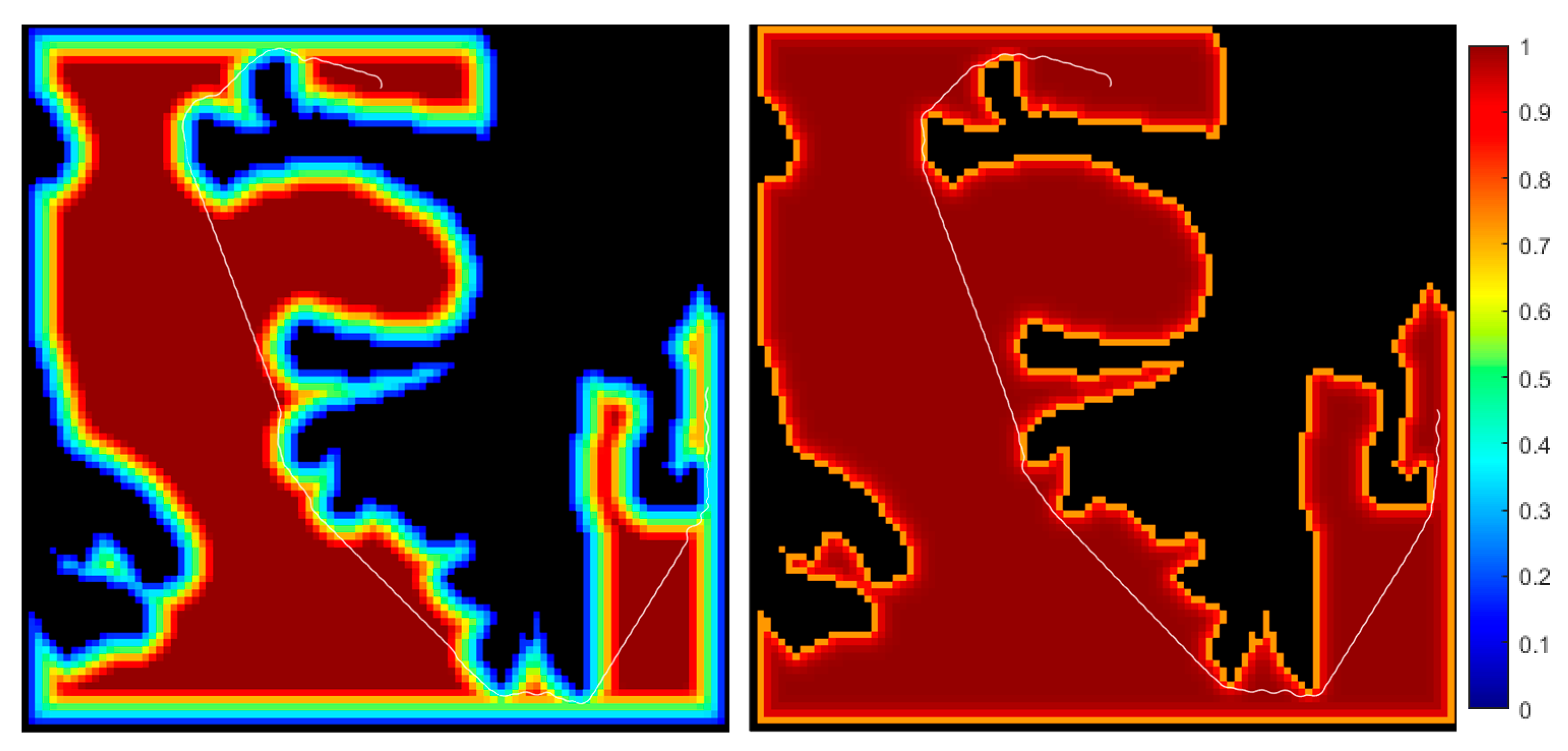
In the global simulation, the map environment is a scaled-down version of a real coastal map. In this environment, the path planning algorithm must be cautious to avoid collisions with black obstacles. The main challenge lies in navigating from the starting point through these irregular spaces, overcoming numerous obstacles, and ultimately reaching the destination safely. This environment tests the intelligence and flexibility of the path planning algorithm, which should maintain a certain safety distance from obstacles to ensure the AUV’s safety.

Figure 7 shows the results of the motion planning. According to the simulation results, the paths generated by the A*, FMM, and Q-Learning (QL) algorithms have a minimum distance of 0 m from the obstacles, indicating that these algorithms fail to effectively avoid obstacles and pose a direct collision risk. Although their total path lengths are shorter (e.g., 191.1 m for A* and FMM), their safety is severely inadequate for practical scenarios. In contrast, MPC-FMCBF maintains a safe distance (1.86 m) while only increasing the path length to 195.2 m, significantly outperforming other algorithms in overall performance. Its advantage stems from the synergistic control of dynamic optimization and safety boundaries: by using model predictive control to adjust the path in real-time and adding the obstacle distance control barrier function of the fast marching method as a safety constraint, it avoids collisions while ensuring path efficiency. In summary, the proposed algorithm achieves a path length of 195.2 m, which is only 2.1% longer than the unsafe benchmarks (e.g., A* and FMM). At the same time, it maintains a minimum safe clearance of 1.86 m, compared to 0 m for the traditional methods. This characteristic makes it highly valuable in high-safety-demand fields such as navigation in server underwater environments.

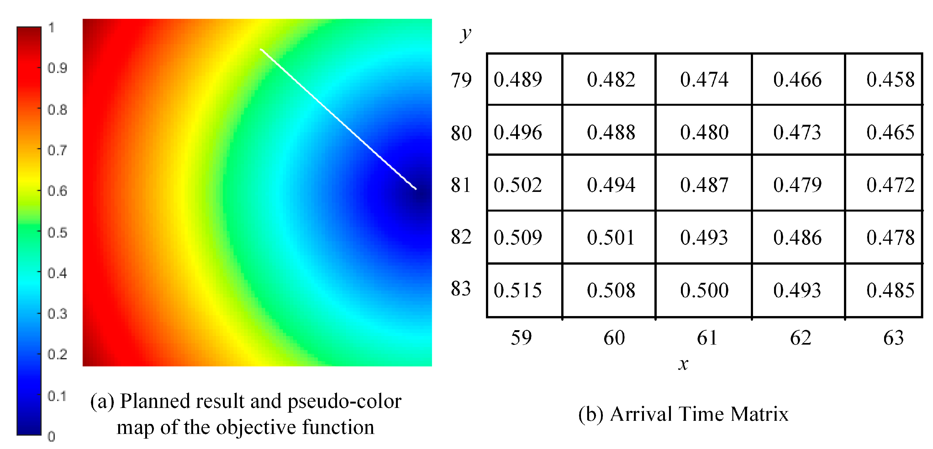
Moreover, both MPC-APFCBF and MPC-FMCBF plan at the speed level. The left image of Figure 8 shows the planning results and the pseudo-color map of the barrier function field for MPC-FMCBF, while the right image of Figure 8 shows the same for MPC-APFCBF. The barrier function field of MPC-FMCBF has a more extensive influence, allowing the path planning to maintain a greater safety distance from obstacles (minimum distance of 1.8583 m, compared to 0.9657 m for MPC-APFCBF), significantly enhancing path safety. Although the path length of MPC-FMCBF is slightly longer (195.2 m compared to 190.4 m for MPC-APFCBF), its smoothness and safety margin are higher, making it more suitable for complex environments. Additionally, MPC-FMCBF avoids the issue of being too close to obstacles seen in MPC-APFCBF, demonstrating higher robustness and reliability.

6.2. Local Motion Planning in Narrow Waterways

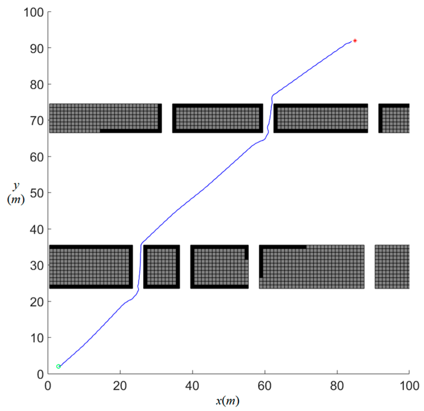
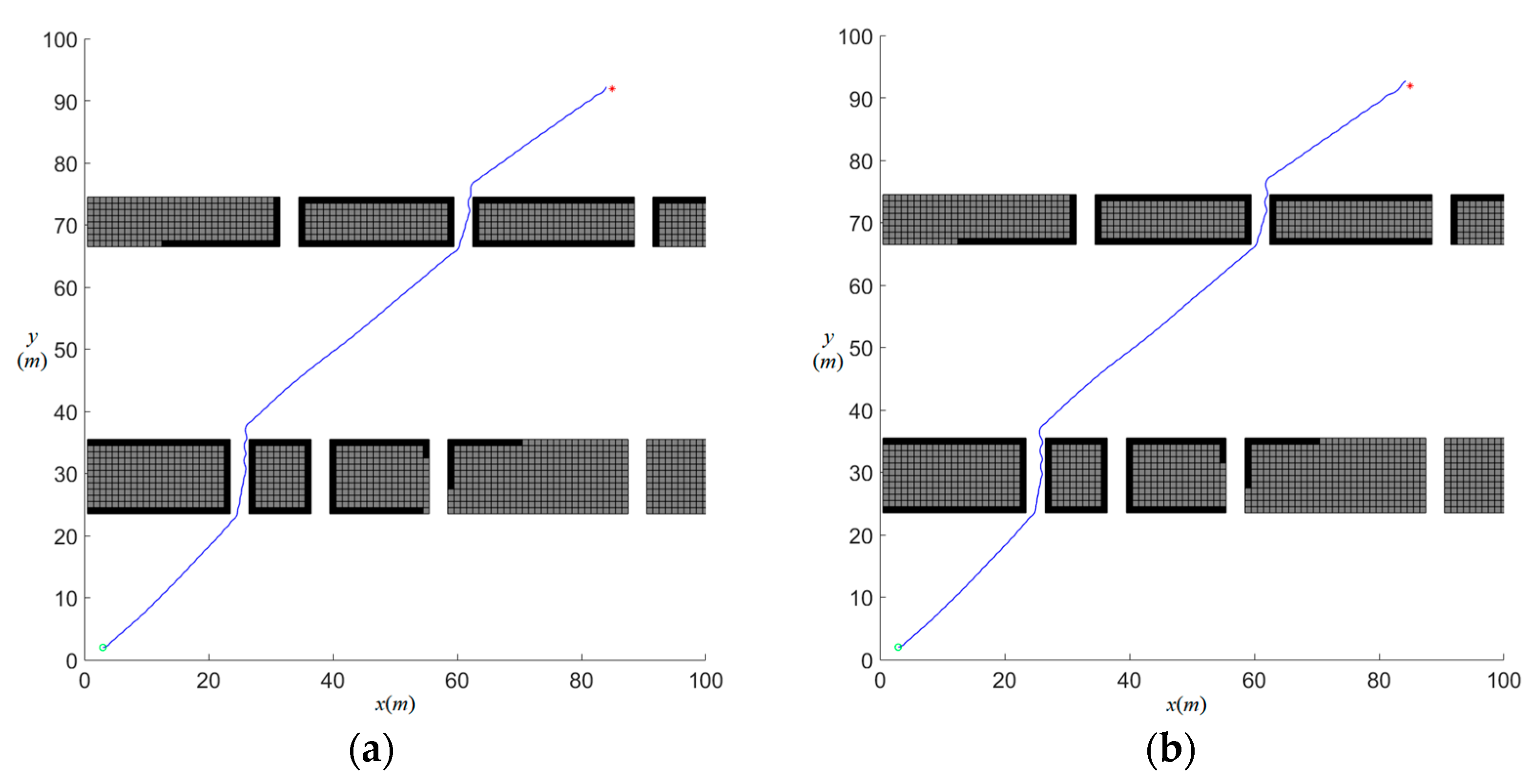
In a narrow waterway environment with artificial constructions, the AUV starts from position (3,2) and aims to reach position (85,92). The waterway features narrow channels with a consistent gap of 3 m, presenting a challenging scenario for motion planning and obstacle avoidance. Figure 9 presents the results obtained by the proposed algorithm. Figure 10 shows the results obtained by MPC-APFCBF and MPC-DC. In the figures, the green circle indicating the starting position and the red star representing the target position. Blue trajectories represent the AUV’s navigation path, while light and dark black dots denote unknown obstacles and detected known obstacles, respectively. The simulation results for local motion planning are illustrated in the three figures corresponding to the MPC-APFCBF, MPC-DC, and MPC-FMCBF algorithms. Initially, the AUV operates with no prior environmental knowledge, initiating motion planning using all three methods. The MPC-APFCBF [27] and MPC-DC (distance constraint) [24] algorithms exhibit nearly identical planning behaviors, with the control barrier functions of MPC-APFCBF failing to demonstrate effective obstacle anticipation. Both methods trigger abrupt turns only when the AUV is close to obstacles, resulting in trajectories marked by frequent directional fluctuations and poor smoothness. In contrast, the proposed MPC-FMCBF algorithm proactively adjusts the path to maintain a safer distance from obstacles, enabling near-linear navigation through narrow channels. This anticipatory behavior stems from the enhanced control barrier function design, which integrates fast marching-based distance fields to preemptively reshape the trajectory while ensuring minimal path deviation. The comparative results highlight MPC-FMCBF’s superior ability to balance safety and efficiency in cluttered environments.

Furthermore, the MPC-FMCBF framework achieves a minimum safety distance of 0.48 m, significantly outperforming MPC-APFCBF and MPC-DC, which achieve only 0.20 m. The primary factors affecting local motion planning include the sensing range of the sonar and the parameter $\gamma$. Hardware limitations constrain the sensing range of the sonar, and setting it to 30 m is reasonable and aligns with practical scenarios. Therefore, a study on the influence of the parameter $\gamma$ was conducted. Based on simulation results, the impact of $\gamma$ can be summarized as follows: as $\gamma$ increases, the safety distance decreases. When $\gamma =0.035$, the safety distance in this narrow navigation channel is 0.48 m. When $\gamma$ = 0.15, the safety distance in the same channel decreases to 0.29 m. At $\gamma$ = 0.35, the results become nearly identical to those of MPC-APFCBF, as the lack of early obstacle avoidance leads to multiple sudden turns and a further reduction in the safety distance to 0.20 m.

6.3. Local Motion Planning in Environments with Dynamic Obstacles

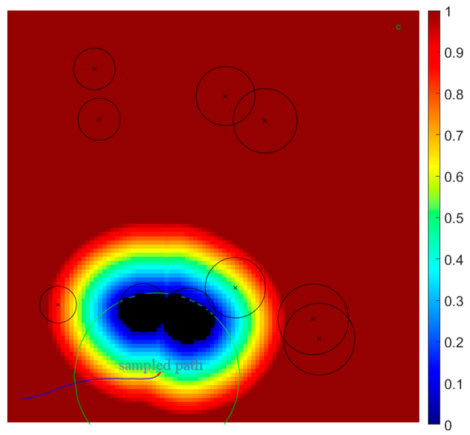
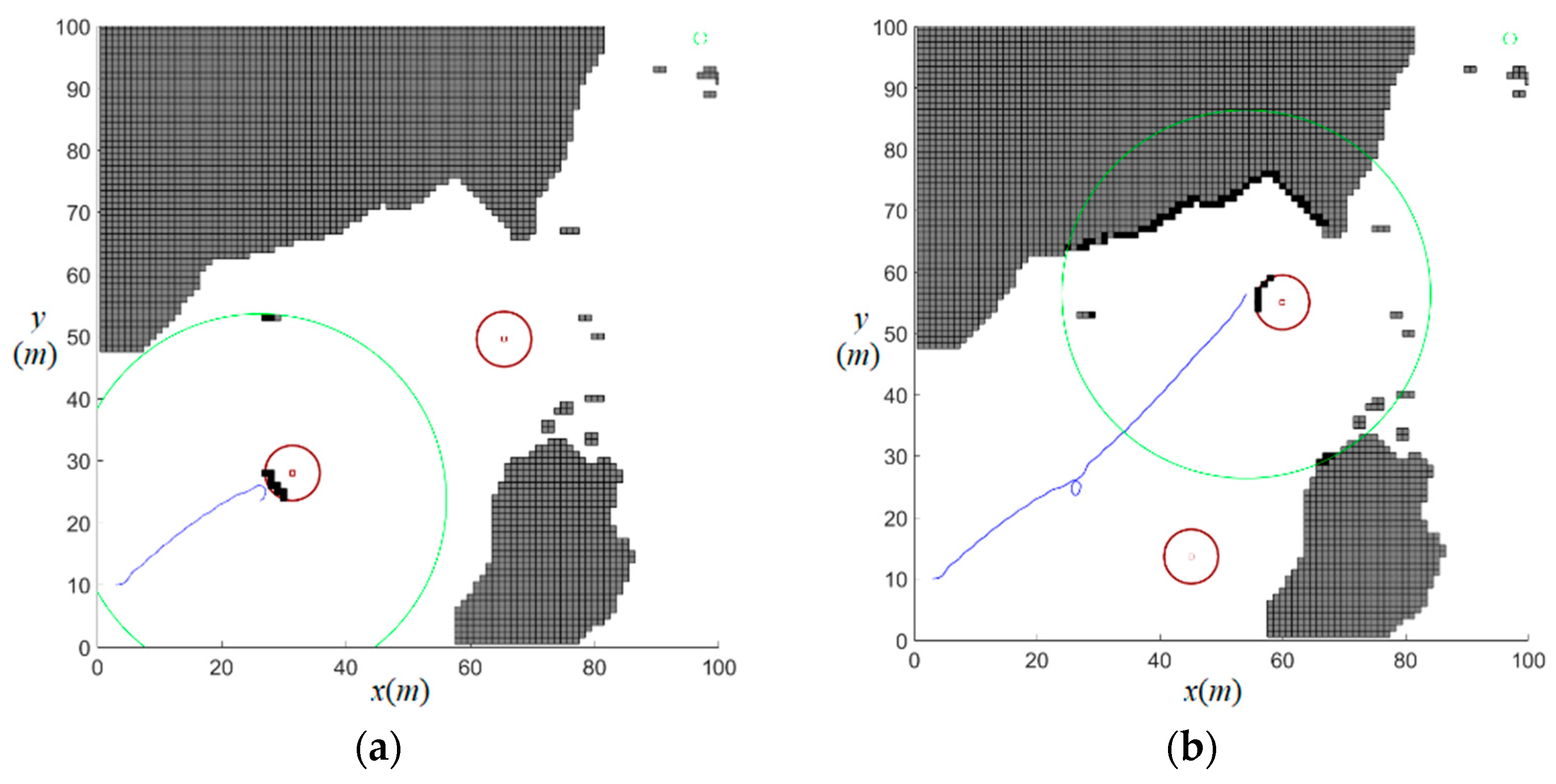
A comprehensive simulation study was conducted to evaluate motion planning performance for an AUV navigating from (3,10) to (97,98) within a 100 m × 100 m dynamic environment containing moving obstacles. Two moving obstacles are set in the simulation represented by red circles in Figure 11 and Figure 12. The speed vectors of the moving obstacles are set to [−0.2, 0.2] m/s and [0.5, −0.525] m/s, representing their velocities in the x and y directions, respectively. Figure 11 and Figure 12 present the comparative motion planning results using MPC-FMCBF and MPC-APFCBF in dynamic scenarios. In the figures, the big green circles indicate the detection region of the AUV’s sonar, and the small green circles denote the target position. 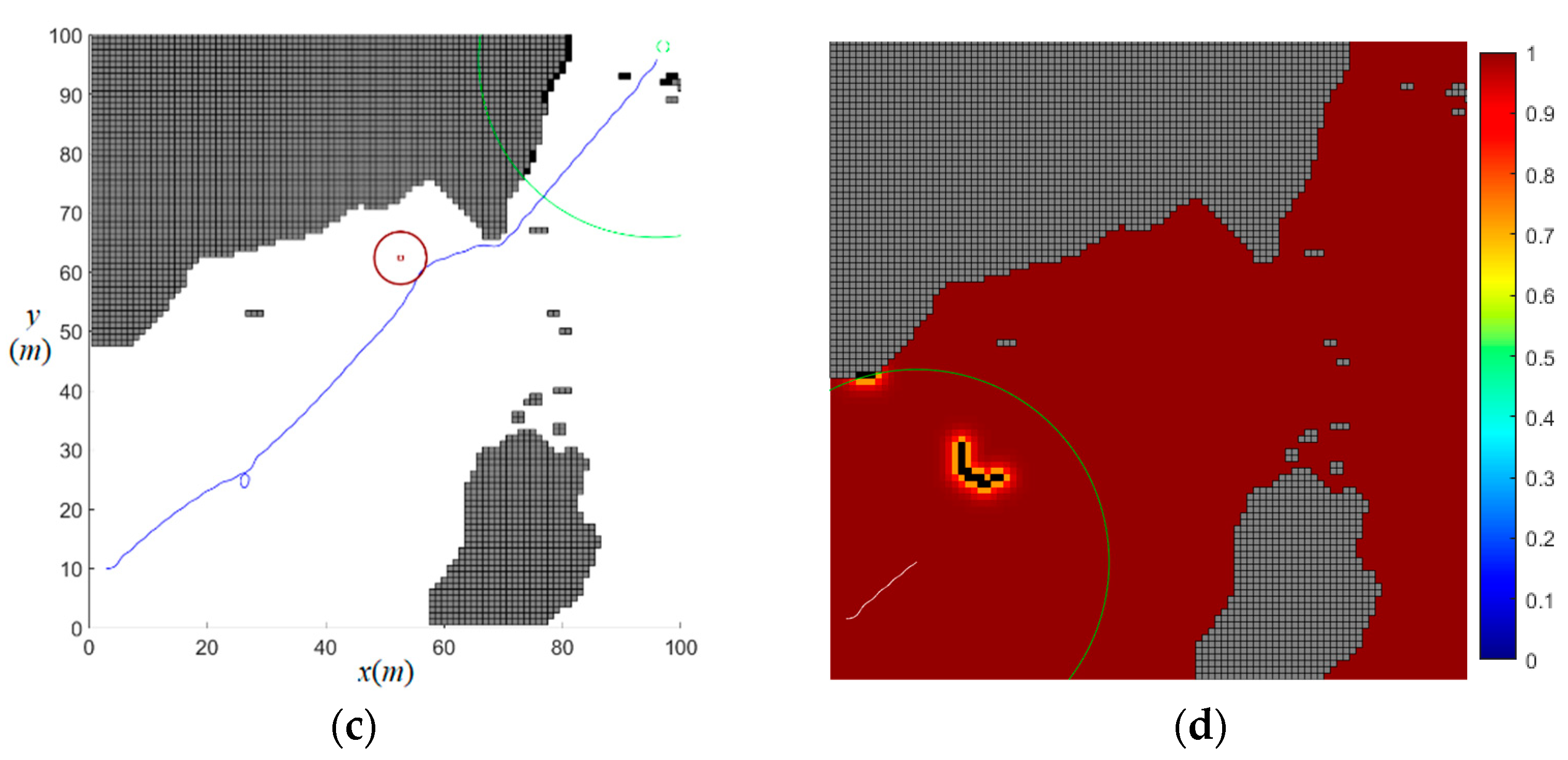Figure 11d illustrates the control barrier function field for dynamic obstacles computed through the FM algorithm. The proposed MPC-FMCBF algorithm enhances obstacle avoidance by strategically increasing grid velocity in the direction of obstacle movement during FM-based distance computation, thereby reducing effective distance values and extending the propagation range of the truncated barrier function field. This innovative approach enables earlier detection and more effective avoidance of moving obstacles.

In contrast, the MPC-APFCBF algorithm’s control barrier function exhibits limited influence, primarily affecting only the immediate grid surrounding the obstacle (as shown in Figure 12d). Figure 12a demonstrates that the AUV using MPC-APFCBF initially moves directly toward the moving obstacle without proactive avoidance, executing abrupt turns only at proximity, which poses significant safety risks in practical applications. While the MPC-FMCBF planned trajectory requires 100.22 s compared to MPC-APFCBF’s 95.96 s, it maintains a safer minimum obstacle distance of 1.76 m versus MPC-APFCBF’s precarious 0.13 m clearance, which nearly results in collision.

In summary, the framework maintains a minimum safety margin of 1.76 m in dynamic scenarios, compared to 0.13 m for MPC-APFCBF, which nearly results in collisions. The comparative results underscore MPC-FMCBF’s exceptional safety performance in dynamic environments, showcasing its unique ability to harmonize path efficiency with robust collision avoidance capabilities, even with marginally increased navigation durations. This strategic trade-off is well-justified by the algorithm’s substantially enhanced safety margins and proactive obstacle anticipation, establishing MPC-FMCBF as the preferred solution for real-world AUV deployments where operational safety constitutes the highest priority. The algorithm’s design philosophy prioritizes guaranteed collision-free navigation over minimal time optimization, aligning perfectly with the critical safety requirements of autonomous underwater operations in complex, unpredictable environments.

Finally, an in-depth analysis of the proposed algorithm’s computational complexity and parameter uncertainty tolerance will be conducted. In terms of computational complexity, the algorithm primarily depends on the FMM and the prediction and optimization steps in the temporal domain during the rolling optimization process of MPC. Assuming the environmental map size is d × d grid cells, the time complexity of the FMM algorithm is O (d²log(d)). This study employs “fmincon-sqp” as the optimization solver, whose typical time complexity is O (k(n² + m³)), where k represents the number of iterations (usually less than 100 in the motion planning optimization problem of this study), n is the number of variables (set to 2), and m is the number of constraints (set to 4). Therefore, for the optimization problem in this study, the time complexity of the optimization solver is relatively low, and the overall computational complexity of the algorithm mainly depends on the execution efficiency of the FMM algorithm.

In terms of robustness, the algorithm demonstrates excellent performance. By adopting a robust MPC framework, only the kinematic model of the AUV is considered during the motion planning process, effectively avoiding the impact of AUV dynamic parameter uncertainties on the planning results. This design strategy significantly enhances the algorithm’s adaptability to system parameter variations, ensuring the reliability of the planning scheme in practical applications.

7. Conclusions

This study proposes a robust Model Predictive Control (MPC) framework for Autonomous Underwater Vehicle (AUV) motion planning in complex environments. The framework integrates a Fast Marching (FM)-based Arrival Time Map and an enhanced Obstacle Avoidance Map, which strategically increases grid propagation speed in the direction of dynamic obstacles, thereby extending the influence of barrier constraints. Extensive simulations demonstrate the framework’s effectiveness in ensuring collision-free navigation and timely target achievement in scenarios involving static and dynamic obstacles, as well as narrow channels. These results highlight significant advancements in AUV safety and operational efficiency.

However, several challenges remain unaddressed. First, the computational scalability of the algorithm needs further optimization to support real-time applications in large-scale environments. Second, the framework currently assumes perfect knowledge of dynamic obstacle trajectories, leaving uncertainties in real-world scenarios unaddressed. Third, the study lacks experimental validation, as the results are based solely on simulations.

To address these limitations, future work will focus on three key directions: (1) enhancing robustness to environmental uncertainties, particularly in dynamic obstacle prediction and sensor noise; (2) conducting field tests to validate the framework’s performance in real-world underwater environments; and (3) integrating advanced perception systems, such as machine learning-based sensors, to improve obstacle detection and avoidance capabilities. These efforts aim to bridge the gap between simulation and practical deployment, further advancing the applicability of the proposed framework in real-world AUV operations.

References

1. Fan, Y.; Dong, H.; Zhao, X.; Denissenko, P. Path-Following Control of Unmanned Underwater Vehicle Based on an Improved TD3 Deep Reinforcement Learning. IEEE Trans. Control Syst. Technol. 2024, 32, 1904–1919. [Google Scholar]
2. Manhães, M.M.M.; Scherer, S.A.; Voss, M.; Douat, L.R.; Rauschenbach, T. AUV Simulator: A Gazebo-based package for underwater intervention and multi-robot simulation. In Proceedings of the OCEANS 2016 MTS/IEEE Monterey, Monterey, CA, USA, 19–23 September 2016; pp. 1–8. [Google Scholar]
3. Zeng, Z.; Sammut, K.; Lian, L.; He, F.; Lammas, A.; Tang, Y. A comparison of optimization techniques for AUV path planning in environments with ocean currents. Robot. Auton. Syst. 2016, 82, 61–72. [Google Scholar]
4. Zhu, D.; Sun, J. A New Algorithm Based on Dijkstra for Vehicle Path Planning Considering Intersection Attribute. IEEE Access 2021, 9, 19761–19775. [Google Scholar]
5. He, P.-F.; Fan, P.-F.; Wu, S.-E.; Zhang, Y. Research on Path Planning Based on Bidirectional A* Algorithm. IEEE Access 2024, 12, 109625–109633. [Google Scholar]
6. Novosad, M.; Penicka, R.; Vonasek, V. CTopPRM: Clustering Topological PRM for Planning Multiple Distinct Paths in 3D Environments. IEEE Robot. Autom. Lett. 2023, 8, 7336–7343. [Google Scholar]
7. Xiao, C.; Yang, H.; Zhang, B. Multi-Unmanned Aerial Vehicle Path Planning Based on Improved Nutcracker Optimization Algorithm. Drones 2025, 9, 116. [Google Scholar] [CrossRef]
8. Ma, Y.-N.; Gong, Y.-J.; Xiao, C.-F.; Gao, Y.; Zhang, J. Path Planning for Autonomous Underwater Vehicles: An Ant Colony Algorithm Incorporating Alarm Pheromone. IEEE Trans. Veh. Technol. 2019, 68, 141–154. [Google Scholar]
9. Chen, M.; Zhu, D. Optimal Time-Consuming Path Planning for Autonomous Underwater Vehicles Based on a Dynamic Neural Network Model in Ocean Current Environments. IEEE Trans. Veh. Technol. 2020, 69, 14401–14412. [Google Scholar] [CrossRef]
10. Lin, C.; Cheng, Y.; Wang, X.; Yuan, J.; Wang, G. Transformer-Based Dual-Channel Self-Attention for AUV Autonomous Collision Avoidance. IEEE Trans. Intell. Veh. 2023, 8, 2319–2331. [Google Scholar]
11. He, Z.; Dong, L.; Sun, C.; Wang, J. Asynchronous Multithreading Reinforcement-Learning-Based Path Planning and Tracking for Unmanned Underwater Vehicle. IEEE Trans. Syst. Man Cybern. Syst. 2022, 52, 2757–2769. [Google Scholar]
12. Yan, J.; Cao, W.; Yang, X.; Chen, C.; Guan, X. Communication-Efficient and Collision-Free Motion Planning of Underwater Vehicles via Integral Reinforcement Learning. IEEE Trans. Neural Netw. Learn. Syst. 2024, 35, 8306–8320. [Google Scholar] [CrossRef]
13. Farhad, B.; Sepideh, N.; Morteza, A. Mobile robots path planning: Electrostatic potential field approach. Expert Syst. Appl. 2011, 100, 68–78. [Google Scholar]
14. Fan, J.; Huang, N.; Huang, D.; Kong, Y.; Chen, Z.; Zhang, F.; Zhang, Y. An Improved Path Planning Algorithm With Adaptive Parameters and Predictions. IEEE Syst. J. 2023, 17, 4911–4921. [Google Scholar] [CrossRef]
15. Li, K.; Zhang, X.; Han, Y. Robot Path Planning Based on Interval Type-2 Fuzzy Controller Optimized by an Improved Aquila Optimization Algorithm. IEEE Access 2023, 11, 111655–111671. [Google Scholar] [CrossRef]
16. Wei, H.; Shi, Y. MPC-based motion planning and control enables smarter and safer autonomous marine vehicles: Perspectives and a tutorial survey. IEEE/CAA J. Autom. Sin. 2023, 10, 8–24. [Google Scholar] [CrossRef]
17. Shen, C.; Shi, Y.; Buckham, B. Model predictive control for an AUV with dynamic path planning. In Proceedings of the 2015 54th Annual Conference of the Society of Instrument and Control Engineers of Japan (SICE), Hangzhou, China, 28–30 July 2015; pp. 475–480. [Google Scholar]
18. Shen, C.; Shi, Y.; Buckham, B. Integrated Path Planning and Tracking Control of an AUV: A Unified Receding Horizon Optimization Approach. IEEE/ASME Trans. Mechatron. 2017, 22, 1163–1173. [Google Scholar] [CrossRef]
19. Chen, M.; Zhu, D.; Pang, W.; Chen, Q. An Effective Strategy for Distributed Unmanned Underwater Vehicles to Encircle and Capture Intelligent Targets. IEEE Trans. Ind. Electron. 2024, 71, 12570–12580. [Google Scholar] [CrossRef]
20. Zheng, H.; Sun, Y.; Zhang, G.; Zhang, L.; Zhang, W. Research on Real Time Obstacle Avoidance Method for AUV Based on Combination of ViT-DPFN and MPC. IEEE Trans. Instrum. Meas. 2024, 73, 5009115. [Google Scholar] [CrossRef]
21. Ames, A.; Xu, X.; Grizzle, J.W.; Tabuada, P. Control Barrier Function Based Quadratic Programs for Safety Critical Systems. IEEE Trans. Autom. Control 2017, 62, 3861–3876. [Google Scholar] [CrossRef]
22. Esfahani, H.N.; Velni, J.M. Safe MPC-based Motion Planning of AUVs Using MHE-based Approximate Robust Control Barrier Functions. In Proceedings of the 2024 32nd Mediterranean Conference on Control and Automation (MED), Chania, Greece, 11–14 June 2024; pp. 161–166. [Google Scholar]
23. Zeng, J.; Li, Z.; Sreenath, K. Enhancing Feasibility and Safety of Nonlinear Model Predictive Control with Discrete-Time Control Barrier Functions. In Proceedings of the 2021 60th IEEE Conference on Decision and Control (CDC), Austin, TX, USA, 13–17 December 2021; pp. 6137–6144. [Google Scholar]
24. Quan, Y.S.; Kim, J.S.; Chung, C.C. Robust Model Predictive Control with Control Barrier Function for Nonholonomic Robots with Obstacle Avoidance. In Proceedings of the 2021 21st International Conference on Control, Automation and Systems (ICCAS), Jeju, Republic of Korea, 12–15 October 2021; pp. 1377–1382. [Google Scholar]
25. Thirugnanam, A.; Zeng, J.; Sreenath, K. Safety-Critical Control and Planning for Obstacle Avoidance between Polytopes with Control Barrier Functions. In Proceedings of the 2022 International Conference on Robotics and Automation (ICRA), Philadelphia, PA, USA, 19–23 May 2022; pp. 286–292. [Google Scholar]
26. Ghanbarpour, M.; Isaly, A.; Sanfelice, R.G.; Dixon, W.E. Optimal Safety for Constrained Differential Inclusions Using Nonsmooth Control Barrier Functions. IEEE Control Syst. Lett. 2023, 7, 1303–1308. [Google Scholar] [CrossRef]
27. Singletary, A.; Klingebiel, K.; Bourne, J.; Browning, A.; Tokumaru, P.; Ames, A. Comparative Analysis of Control Barrier Functions and Artificial Potential Fields for Obstacle Avoidance. In Proceedings of the 2021 IEEE/RSJ International Conference on Intelligent Robots and Systems (IROS), Prague, Czech Republic, 27 September–1 October 2021; pp. 8129–8136. [Google Scholar]
28. Yang, Z.; Yan, S.; Ming, C.; Wang, X. Intelligent Dynamic Trajectory Planning of UAVs: Addressing Unknown Environments and Intermittent Target Loss. Drones 2024, 8, 721. [Google Scholar] [CrossRef]
29. Yazdani, A.; MahmoudZadeh, S.; Yakimenko, O.; Wang, H. Perception-aware online trajectory generation for a prescribed manoeuvre of unmanned surface vehicle in cluttered unstructured environment. Robot. Auton. Syst. 2023, 169, 104508. [Google Scholar] [CrossRef]
30. Li, X.; Yu, S.; Gao, X.-Z.; Yan, Y.; Zhao, Y. Path planning and obstacle avoidance control of UUV based on an enhanced A* algorithm and MPC in dynamic environment. Ocean Eng. 2024, 302, 117584. [Google Scholar] [CrossRef]
31. Fossen, T. Handbook of Marine Craft Hydrodynamics and Motion Control; Wiley: Oxford, UK, 2011. [Google Scholar]
32. Yang, C.; Pan, J.; Wei, K.; Lu, M.; Jia, S. A novel unmanned surface vehicle path-planning algorithm based on A* and artificial potential field in ocean currents. J. Mar. Sci. Eng. 2024, 12, 285. [Google Scholar] [CrossRef]
Figure 1. Earth-fixed and body-fixed frames.
Drones 09 00273 g001
Figure 2. Robust model predictive control framework for motion planning.
Drones 09 00273 g002
Figure 3. Update process of fast marching algorithm. (a). Initialization phase. The arrival time at the starting point is set to 0, and the starting point is marked as a Known point (black sphere). (b). First iteration. The four neighboring points around the starting point are identified as Trial points (orange spheres), and their tentative arrival times are calculated. (c). The right neighboring point of the starting point is selected as the next Known point, and its adjacent points are updated to Trial points. (d). The point below the starting point is selected as the next Known point, and its adjacent points are updated to Trial points. (e). The top neighboring point of the starting point is selected as the next Known Point, and its adjacent points are updated to Trial points. (f). The left neighboring point of the starting point is selected as the next Known point, completing the initial wavefront propagation.
Drones 09 00273 g003
Figure 4. Obstacle avoidance map generation.
Drones 09 00273 g004
Figure 5. Safety and obstacle avoidance capability.
Drones 09 00273 g005
Figure 6. Convergence analysis illustration.
Drones 09 00273 g006
Figure 7. Global planning comparison.
Drones 09 00273 g007
Figure 8. Pseudo-color maps of control barrier function fields for MPC-APFCBF and MPC-FMCBF.
Drones 09 00273 g008
Figure 9. Local motion planning in a narrow waterway by the proposed algorithm.
Drones 09 00273 g009
Figure 10. Local motion planning in a narrow waterway by (a) MPC-APFCBF and (b) MPC-DC.
Drones 09 00273 g010
Figure 11. Local motion planning with moving obstacles by MPC-FMCBF. (a) At the step of 20 s. (b) At the step of 55 s. (c) At the step of 95 s. (d) Control barrier function field by FM.
Drones 09 00273 g011
Figure 12. Local motion planning with moving obstacles by MPC-APFCBF. (a) At the step of 20 s. (b) At the step of 55 s. (c) At the step of 95 s. (d) Control barrier function field by APF.
Drones 09 00273 g012aDrones 09 00273 g012b