Real-Time Optimal Control Design for Quad-Tilt-Wing Unmanned Aerial Vehicles

Abstract

Quad-tilt-wing (QTW) Unpiloted Aerial Vehicles (UAVs) combine the vertical takeoff and landing capabilities of rotary-wing designs with the high-speed, long-range performance of fixed-wing aircraft, offering significant advantages in both civil and military applications. The unique configuration of QTW UAVs presents complex control challenges due to nonlinear dynamics, strong coupling between translational and rotational motions, and significant variations in aerodynamic characteristics during transitions between flight modes. To address these challenges, this study develops an optimal control framework tailored for real-time operations. A State-Dependent Riccati Equation (SDRE) approach is employed for attitude control, addressing nonlinearities, while a Linear Quadratic Regulator (LQR) is used for position and velocity control to achieve robustness and optimal performance. By integrating these strategies and utilizing the inverse dynamics approach, the proposed control system ensures stable and efficient operation. This work provides a solution to the optimal control complexities of QTW UAVs, advancing their applicability in demanding and dynamic operational environments.

1. Introduction

Advancements in unpiloted aerial vehicles (UAVs) have made significant progress in recent years due to their diverse applications in areas such as environmental monitoring, structural inspection, and disaster response [1,2,3]. Conventional UAVs are commonly categorized into fixed-wing and rotary-wing groups. Each category presents unique advantages and constraints [2]. Fixed-wing UAVs are highly effective in high-speed, long-range flight; however, they require runways for takeoff and landing. In contrast, rotary-wing UAVs, such as quadcopters, can hover, perform complex maneuvers, take off or land vertically, and consume less energy in hover. However, they have lower cruising speeds and range [3].

To address the above-mentioned limitations and to maximize the aerodynamic lift effects and optimize forward flight speed while minimizing energy consumption during hover flight, the concept of hybrid UAVs, also known as convertible or convertiplane aircraft, has been developed. These aircraft integrate the vertical takeoff and landing (VTOL) capabilities of rotary-wing UAVs with the high-speed, long-range flight characteristics of fixed-wing designs [4]. Hybrid UAVs have been designed in various types of structures and configurations such as tilt-rotor and tilt-wing variants, each of which has its own set of advantages and trade-offs.

Tilt-rotor UAVs are typically equipped with two or three rotors and a tilt mechanism, which enables them to vertically take off and land as well as fly horizontally. The energy efficiency, stability, and precise controllability of tilt-rotor UAVs make them compelling subjects for research [5]. However, dual-tilt-rotor UAVs require complex cyclic control mechanisms, adding to their mechanical complexity [5] and making them vulnerable to operational failure if one rotor malfunctions [1].

In contrast, tilt-wing UAVs, such as dual-tilt-wing (DTW) and quad-tilt-wing (QTW) UAVs, address these limitations by incorporating tilting rotors integrated with the wings. In the case of QTWs, there are four tilting wings. As a subset of tilt-wing UAVs, the QTW configuration not only enhances redundancy by allowing the aircraft to maintain flight even if one rotor fails but also improves aerodynamic efficiency by taking advantage of the slipstream effect [1]. The tilting wings of QTW UAVs offer a more stable and efficient transition between vertical and horizontal flight modes, making them a more robust solution for applications requiring both VTOL and high-speed cruise capabilities [1]. Also, when compared to traditional quadcopters, the QTW concept offers significant advantages such as enhanced maximum speed, decreased path completion time, reduced energy consumption, increased maximum range, and improved maneuverability [6,7]. Exceptional maneuverability, vertical takeoff, high-speed cruise, and vertical landing are all parts of the QTW UAVs’ successful complete conversion flight that highlight their civil and military application potentials [7,8,9,10].

Designing a controller for the QTW UAV is highly challenging due to its unique configuration and the complex dynamics involved in its operation [10,11]. Achieving precise stabilization and control of the UAV’s attitude is required in the QTW, especially due to the significant variations in aerodynamic characteristics resulting from the wing tilt angle [8,9,10]. This variation adds complexity to the control process, particularly during transitions from VTOL to cruise flight mode and vice versa [2]. Also, during transition flights, the UAV shows highly nonlinear dynamic behavior when the relative wind is not aligned with the wings, therefore presenting further difficulties in maintaining stability and controlling its attitude [3]. 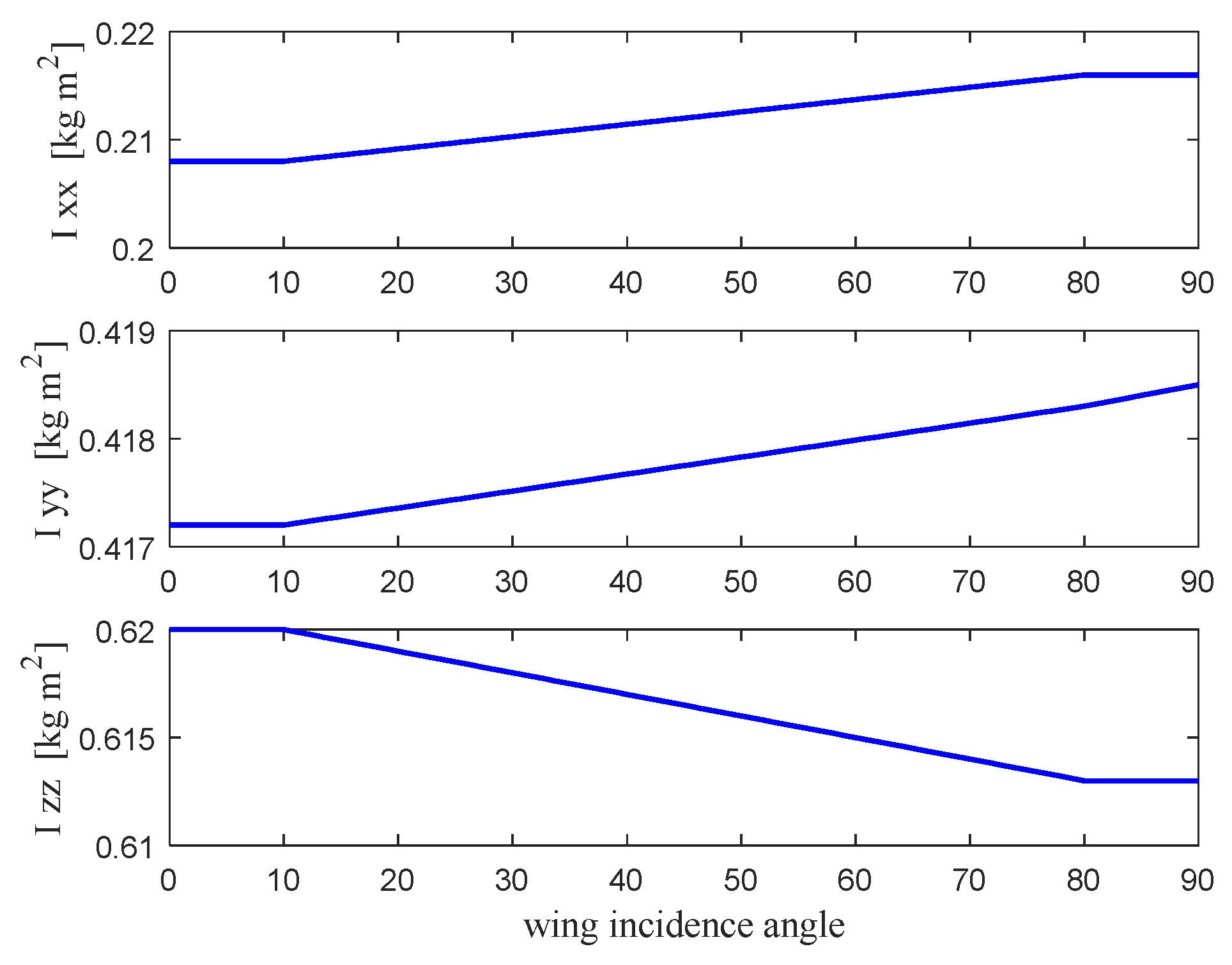Furthermore, the control complexity is further increased by the strong couplings between translational and rotational motions, resulting in a highly nonlinear, multi-input, multi-output system [11]. Moreover, the system must exhibit robustness against a range of uncertainties, including different types of unpredictable damages, actuator failures, and fluctuations in mass moments of inertia during wing tilting [5,11]. Conventional linear controllers designed for fixed-wing UAVs are often inadequate for QTW UAVs due to these nonlinearities and uncertainties. Therefore, advanced control strategies are required to achieve high performance across a broad flight envelope.

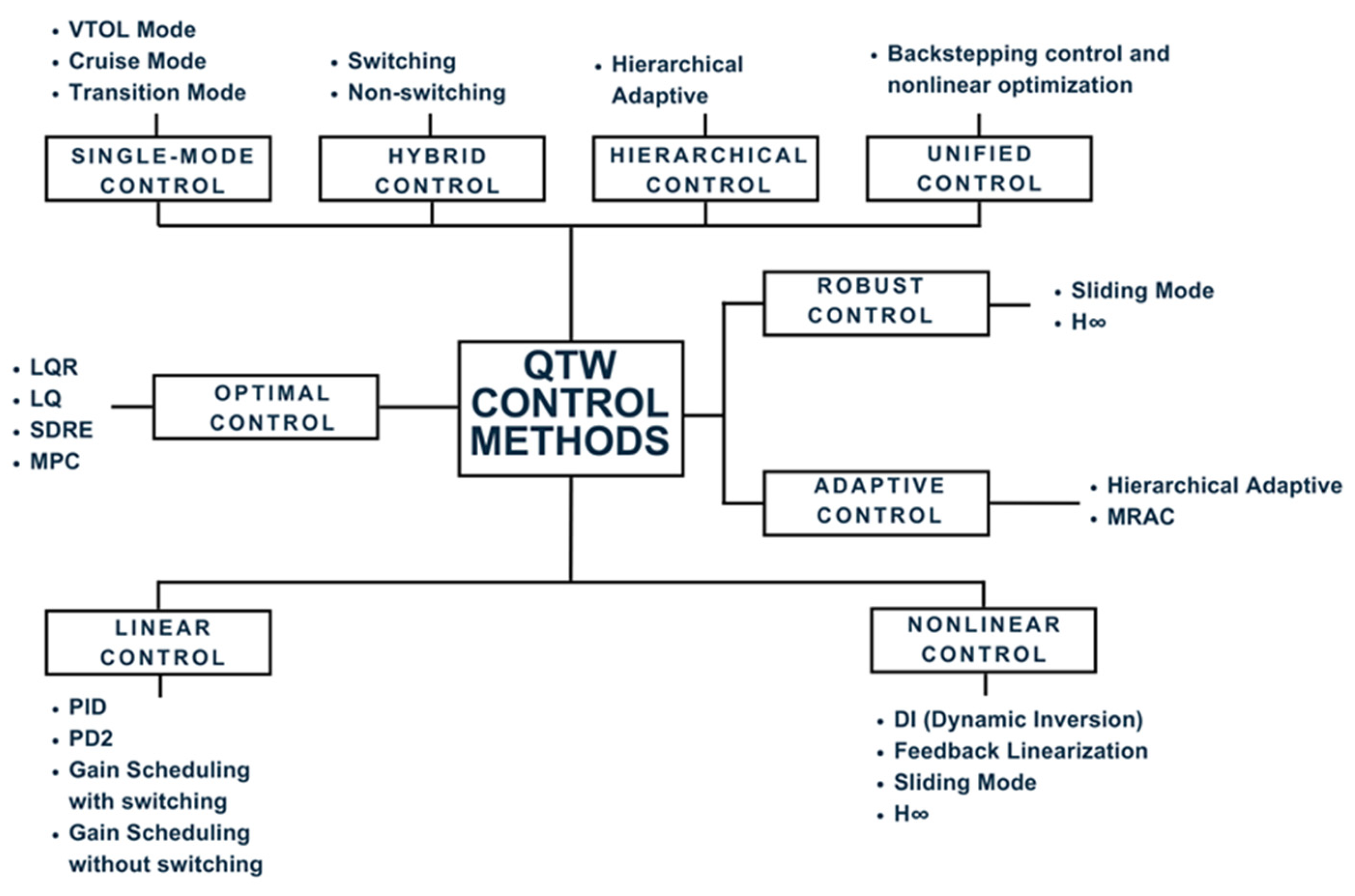
Various control strategies have been proposed in the literature to overcome the above-mentioned challenges. Figure 1 presents the classification of available methods described in the literature.

Some controllers were designed to control the behavior of a QTW UAV in restricted flight conditions, such as VTOL, hovering, or cruising [12,13]. These controllers are easier to design and implement than a general-purpose controller due to their emphasis on a particular set of dynamics [1]. For example, the aerodynamic effects are negligible in hover mode and are simplified terms in cruise phase, which enables the use of simpler control strategies, such as PID controllers [1]. The flexibility and applicability of these controllers in a comprehensive flight scenario are restricted by their inability to manage transitions between flight modes and their potentially poor performance outside of their intended operating conditions [1,14,15,16].

Hybrid controllers such as the one in [17] are proposed as a solution to manage various flight modes by either switching between distinct control algorithms designed for each operational mode or employing a non-switching framework. Switching controllers update their control approach according to the present flying mode. One possible approach is to use separate controllers for hover, transition, and cruise phases, alternating as necessary to enhance performance for each mode; however, the switching process could lead to challenges, such as a decrease in altitude across transitions caused by alterations in controller dynamics and response characteristics [4]. Unified controllers, such as the one presented in [4], are alternatives that are applied to provide a consistent control technique applicable to all flight modes. These approaches employ continuous flight configuration spaces derived from wind tunnel tests [18] or dynamic computations [19], which allow for consistent performance without the need for discrete mode definitions. Eliminating the need for switching between controllers reduces the complexity and potential instability [4].

Certain works, including [5,11], implemented a hierarchical control structure by decomposing the control problem into multiple layers, with lower layers handling fast dynamics such as attitude control (rotational dynamics), and upper layers managing slower dynamics such as position control (translational dynamics). This layered approach allows for specialized controllers at each level, enhancing stability and performance. The hierarchical adaptive control suggested in [11] incorporates adaptive controllers for both translational and rotational motion control, enabling adaptation in all six degrees of freedom. To address uncertainties and dynamic changes in the quad-tilt-wing environment or configuration, [5] proposed a position controller based on the hierarchical adaptive approach. In the suggested method, a model reference adaptive controller is used at a high level to create commands that direct the UAV along a predetermined path. These commands determine the desired attitude angles, which are then transmitted to the lower-level controller.

Several studies have employed linearization-based techniques such as dynamic inversion [20] and Feedback Linearization [21] to design simplified controllers. These approaches significantly depend on precise system models, and they are sensitive to performance deterioration and possible stability problems when the precision of the model is compromised [2]. In [2], an H∞ controller was applied to a linearized system.

Linear controllers such as PIDs [22,23] and gain scheduling [24] are also proposed for this application. Linear controllers are developed using linear approximations of the vehicle dynamics and are appropriate for a particular, well-defined operational point. Nonlinear controllers such as in sliding mode [25,26] are uniquely developed to effectively handle the complicated and nonlinear dynamics of QTW UAVs, thus ensuring robustness and acceptable performance throughout various operational points. The inherent challenge of nonlinear controls is their computational complexity [11]; however, nonlinear robust control approaches are proposed in the literature to deal with the high level of uncertainties.

The objective of optimal control techniques is to solve mathematical optimization problems to optimize a performance criterion, such as lowering energy consumption or maximizing stability.

Many linear optimal control approaches are designed for convertible aircraft, including Linear Quadratic Regulator (LQR), sliding mode control (SMC) [27], Model Predictive Control (MPC) [1], and LQR methods [28]. These control strategies have been implemented with varying degrees of success in addressing the challenges associated with hybrid UAVs.

For instance, an optimal controller was designed in [29] for a Linear Parameter-Varying (LPV) model, whereby the system matrix is variable with the tilt angle. Despite continuous fluctuations in controller gain, the real-time control of the UAV presents issues because of the necessity of solving the Riccati equation to calculate the gain. This creates challenges in maintaining stability and performance during UAVs’ real-time operations.

An MPC-based control system developed in [1] successfully handled the attitude and altitude of a QTW drone, addressing the inherent instability of tail-sitter convertible aircraft while hovering. In contrast to linear control approaches, which are typically insufficient for addressing such instability, the MPC approach has exhibited acceptable efficacy in this situation, providing robustness during the different flight regimes.

Certain techniques, such as dynamic inversion, developed in [20], seek to linearize the model throughout the control procedure, but this technique has limitations: (1) Control inputs can exceed their thresholds due to the elimination of nonlinear components to create a linear model. (2) Discrepancies frequently arise between the real and estimated nonlinear terms, resulting in system instability and decreased control efficacy.

Nonlinear optimal control methods are viable alternatives for addressing these types of issues, as they take into account the system nonlinearity and the constraints on control inputs [3]. The State-Dependent Riccati Equation (SDRE) control method was proposed in [3] for controlling the behavior of QTW-UAV systems. The SDRE approach is employed to solve the Hamilton–Jacobi equation in nonlinear optimal problems. This methodology facilitates the development of a control system that can handle both system nonlinearity and fluctuating parameters, ultimately leading to more reliable performance across varying operating conditions. Solving the SDRE control problem in real time presents significant challenges, rendering it unsuitable for many onboard autopilot processors.

Optimal control techniques such as the State-Dependent Riccati Equation (SDRE) and Linear Quadratic Regulator (LQR) are highly suitable for attaining consistent performance and stability over a broad range of flying conditions. This work presents an optimum control strategy by selecting SDRE for attitude control to address nonlinearities and choosing LQR for position and velocity control to achieve optimal performance and robustness. The resulting control structure is a balanced and effective way for managing QTW UAVs in different flight conditions. An analytical solution for the SDRE is provided, making it well suited for real-time implementation by eliminating the need to resolve the Riccati equation at each time step.

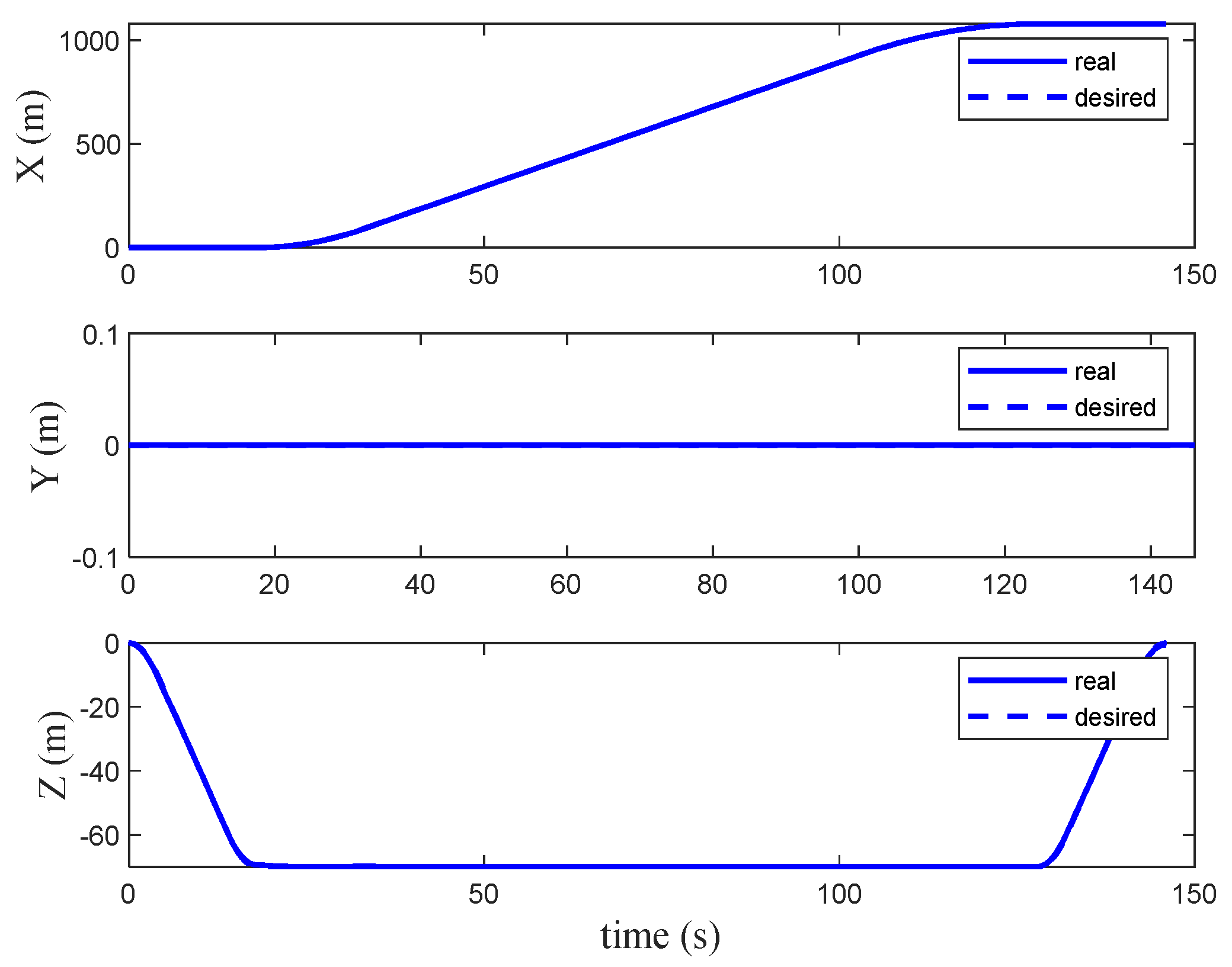
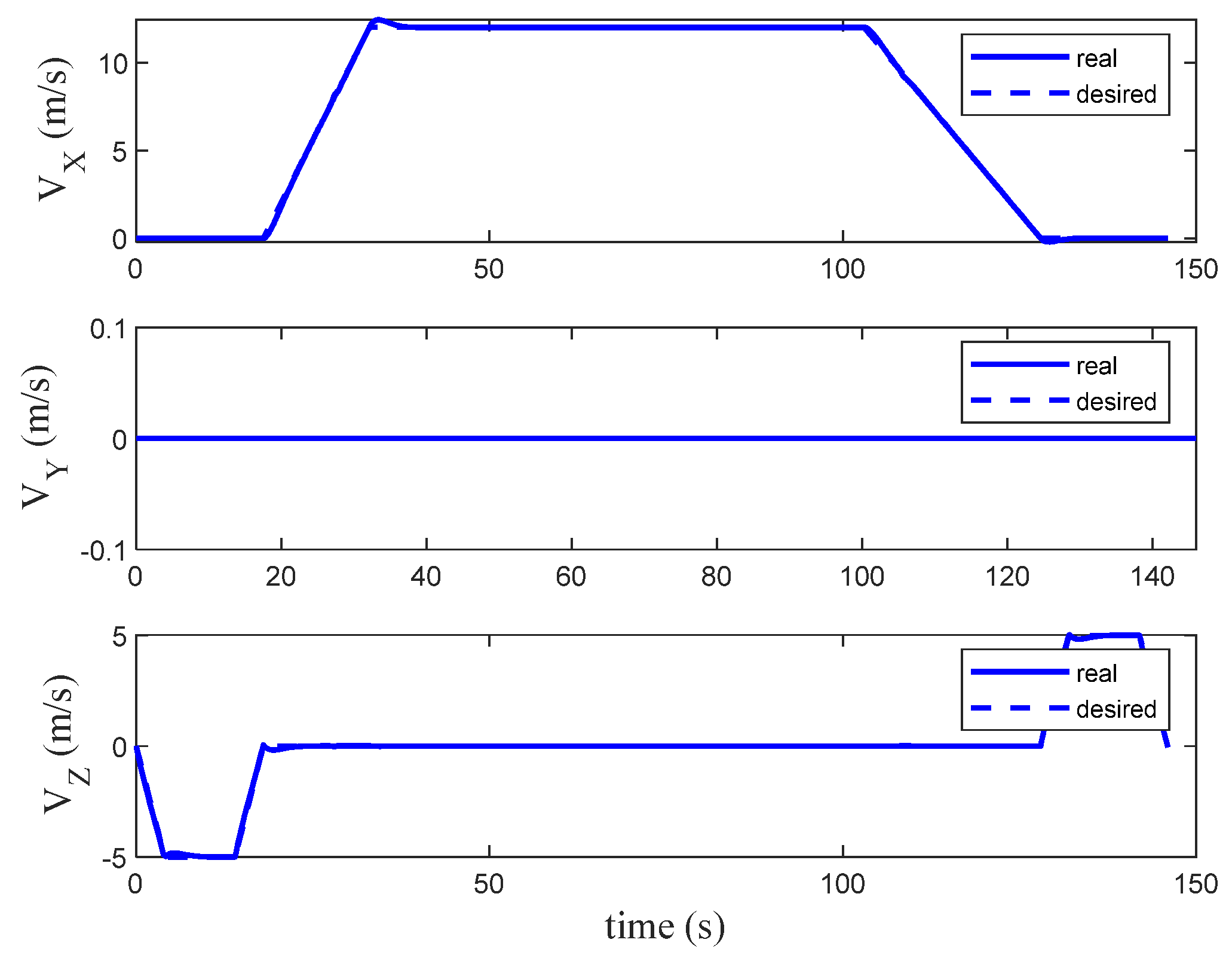
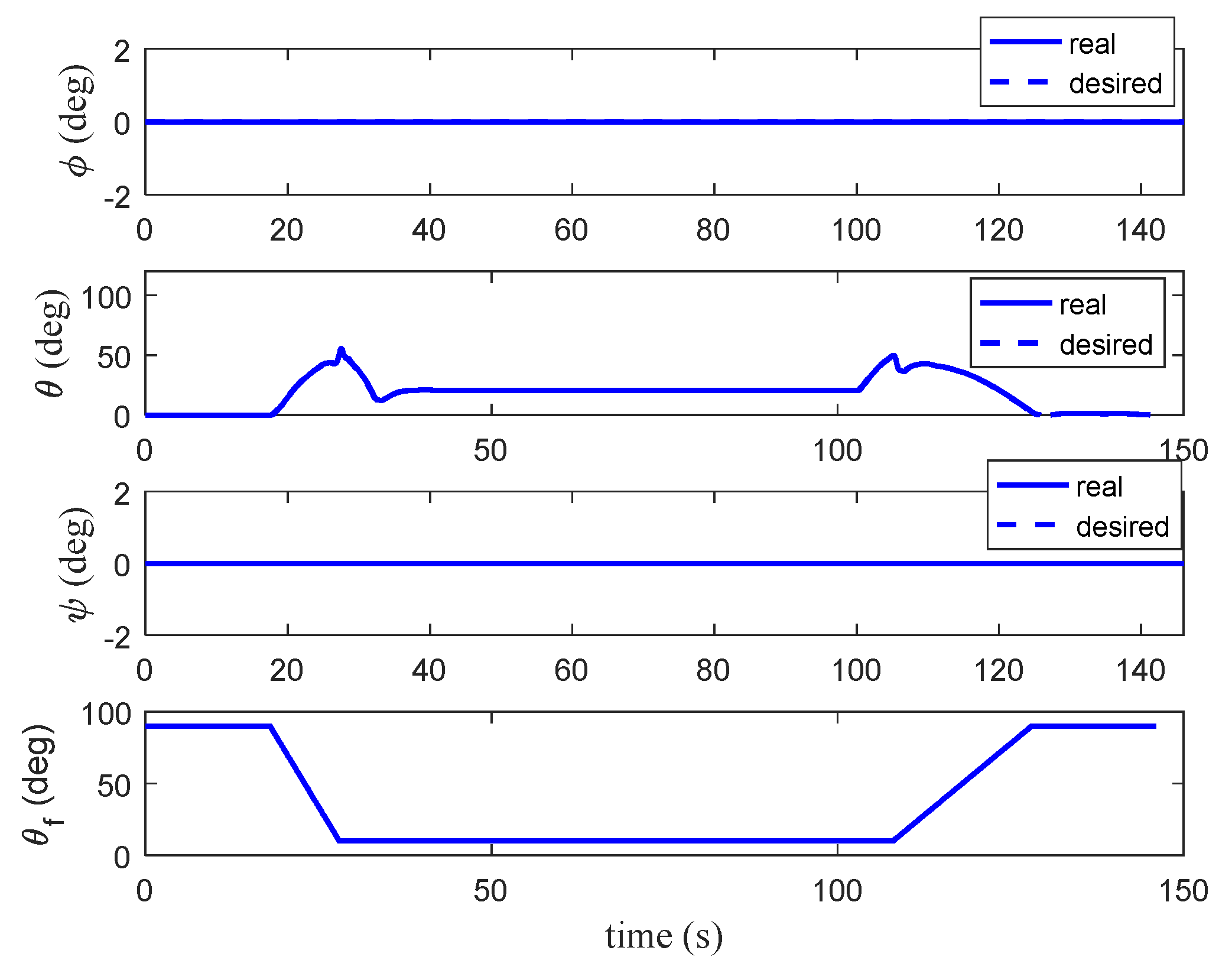
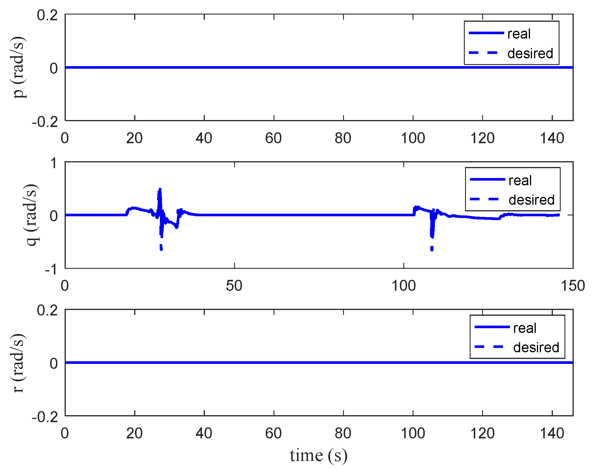
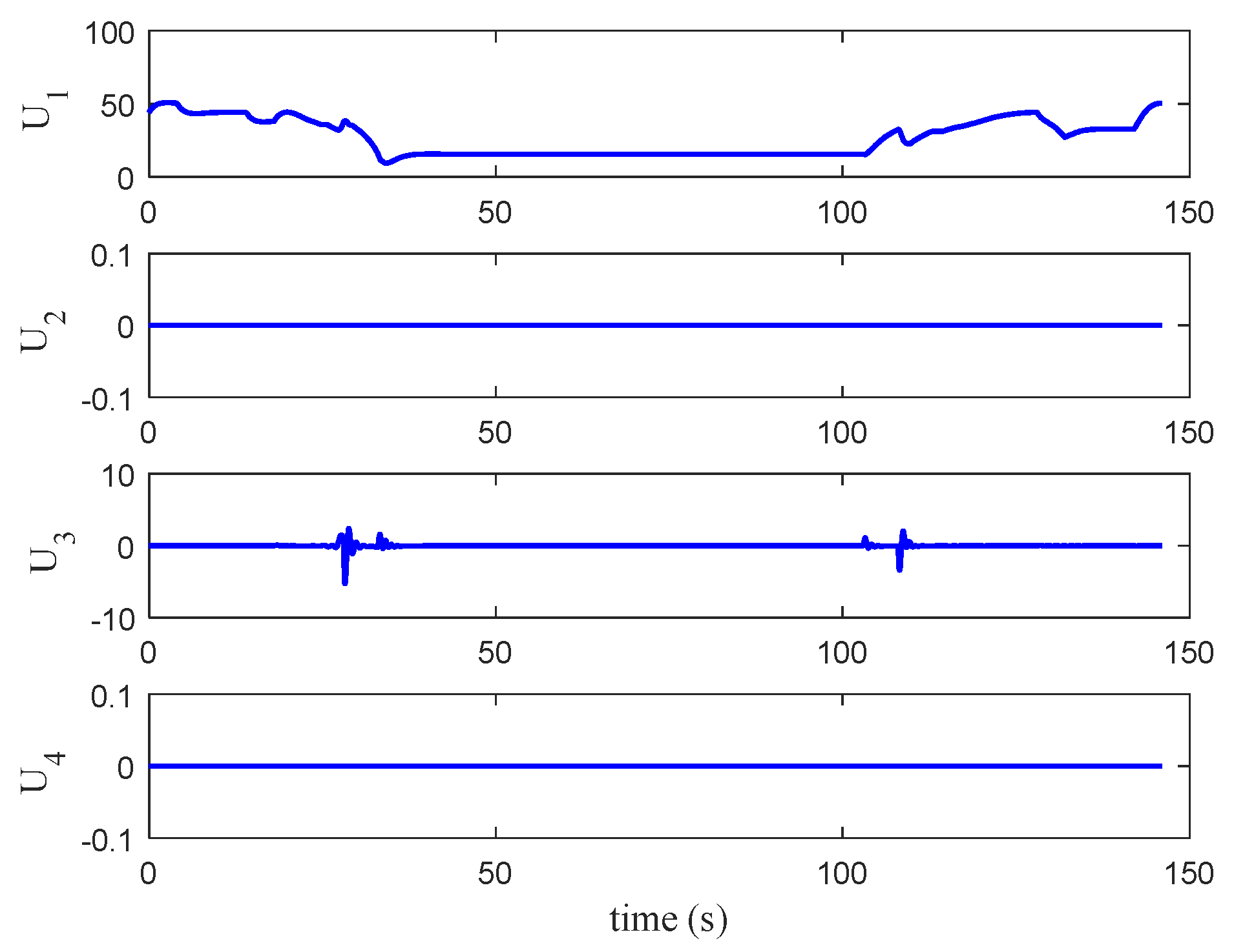
The remainder of this paper is organized as follows: Section 2 presents the dynamic modeling of the quad-tilt-wing system, detailing the equations of motion and system dynamics. Section 3 describes the optimal control design, including the formulation of the control problem and the development of the proposed solution methodology. Section 4 provides simulation results to validate the effectiveness of the proposed control approach and assess system performance. Finally, Section 5 concludes the paper by summarizing the key findings and discussing potential directions for future research.

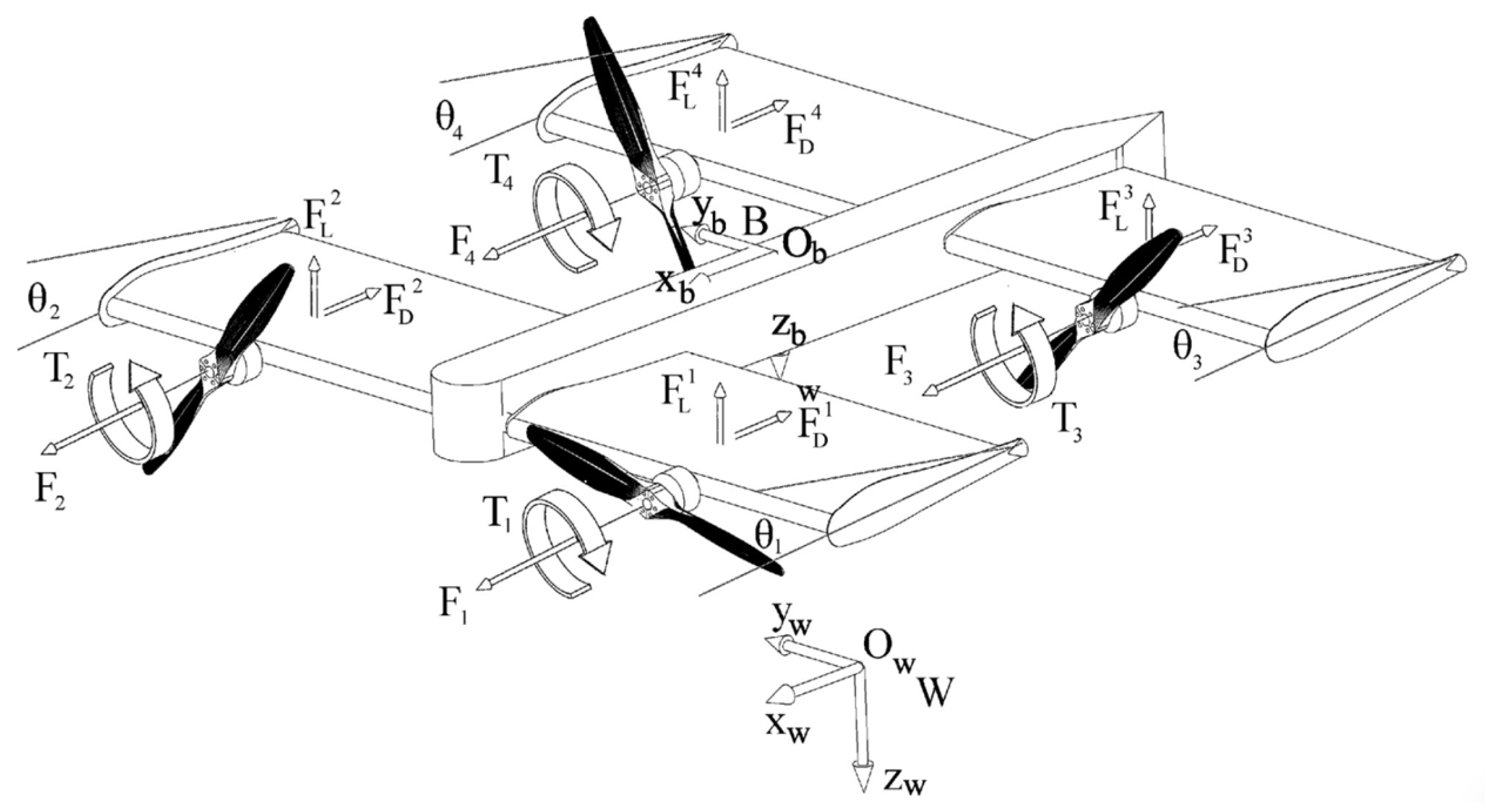
2. QTW Dynamic Modeling

A schematic of the quad-tilt-wing aircraft is illustrated in Figure 2. This configuration consists of four symmetrical wings, each equipped with a motor. Each wing has its own independent tilt mechanism, allowing it to adjust its angle independently of the others.

In this design, motors 1 and 2 are mounted on the front wings, while motors 3 and 4 are located on the rear wings. Motors 2 and 4 are positioned on the right-side wings, and motors 1 and 3 are on the left-side wings. To maintain stability, motors 1 and 4 rotate clockwise, while motors 2 and 3 rotate counterclockwise. The tilt mechanism allows each wing to adjust its installation angle, ${\theta }_i$, between 0° and 90°, thereby independently altering its lift and drag.

The body frame is defined similarly to other aerial vehicles: the $x_b$-axis points toward the nose of the aircraft, the $y_b$-axis points toward the right wing, and the $z_b$-axis points downward.

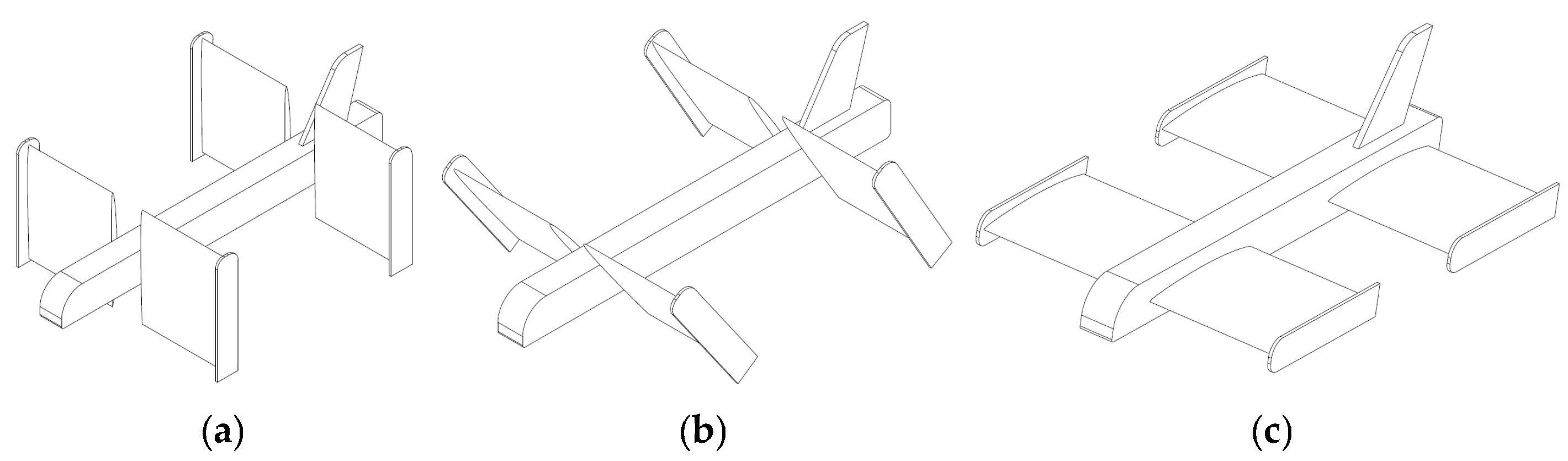
2.1. Flight Envelope

The QTW flight envelope comprises distinct phases: vertical takeoff, transition, cruise, and back transition and vertical landing.

▪

Vertical Takeoff:

During takeoff, the wings are tilted to 90°, enabling the motors to provide vertical thrust. This allows the aircraft to lift off vertically like a conventional multi-rotor drone. After reaching a safe altitude, the transition to forward flight begins.

▪

Transition to Cruise Mode:

In the transition phase, the wing angles gradually decrease from 90° to a forward-tilted position. This adjustment introduces a forward thrust component, enabling the aircraft to accelerate and transition to cruise mode. As the speed increases, the wings begin to generate lift, reducing the thrust required from the motors to support the aircraft’s weight. Once the speed exceeds a safe transition threshold (e.g., 1.2 times the stall speed), the aircraft enters fixed-wing cruise mode.

▪

Cruise Mode:

In cruise mode, the aircraft behaves like a conventional fixed-wing aircraft, with the wings providing the majority of the lift and the motors primarily supplying forward thrust.

▪

Vertical Landing (Back Transition):

To land vertically, the aircraft undergoes a reverse transition. The wing angles are gradually tilted back to 90°, reducing the cruise speed and guiding the aircraft to the landing spot. Once the forward speed is reduced to zero, the motors provide vertical thrust for a controlled, vertical descent.

Figure 3 illustrates the three operational modes of the QTW aircraft: vertical takeoff, transition, and cruise. This flexible configuration enables the QTW to combine the vertical takeoff and landing capabilities of a multi-rotor with the efficient cruise performance of a fixed-wing aircraft.

2.2. Kinematic Modeling

According to the system shown in Figure 2, the world frame $F_w$ with the origin of $O_w$ is defined, as well as the QTW body frame $F_b$ with the origin of $O_b$ located at the QTW center of gravity. The position and velocity of the QTW in the inertial frame are denoted as

$${\mathit{P}}_w={\left[X,Y,Z\right]}^T,{\mathit{V}}_w={\dot{\mathit{P}}}_w={\left[\dot{X},\dot{Y},\dot{Z}\right]}^T.$$

(1)

The Euler angles of the QTW are defined as ${\mathit{\varphi }}_b={\left[\varphi ,\theta ,\psi \right]}^T$, where $\varphi , \theta$, and $\psi$ are the QTW roll, pitch, and yaw angles, respectively.

To define the QTW velocity in the body frame ${\mathit{V}}_b$, it is necessary to derive the transformation between the world frame and the body frame ${\mathit{R}}_{wb}\left(\varphi ,\theta ,\psi \right)$ as

$${\mathit{R}}_{wb}\left(\varphi ,\theta ,\psi \right)=\left[\begin{array}{ccc}{C}_{\psi }{C}_{\theta }& S_{\varphi }{S}_{\theta }{C}_{\psi }-C_{\varphi }{S}_{\psi }& C_{\varphi }{S}_{\theta }{C}_{\psi }+S_{\varphi }{S}_{\psi }\\ S_{\psi }{C}_{\theta }& S_{\varphi }{S}_{\theta }{S}_{\psi }+C_{\varphi }{S}_{\psi }& C_{\varphi }{S}_{\theta }{S}_{\psi }+S_{\varphi }{C}_{\psi }\\ -S_{\theta }& S_{\varphi }{C}_{\theta }& C_{\varphi }{C}_{\theta }\end{array}\right],$$

(2)

where $C(.)$ and $S(.)$ denote cosine and sine, respectively. From ${\mathit{R}}_{wb}$, the QTW velocity in the body frame can be obtained from

$${\mathit{V}}_b=\left[\begin{array}{c}{\upsilon }_x\\ {\upsilon }_y\\ {\upsilon }_z\end{array}\right]={\mathit{R}}_{wb}^T\left(\varphi ,\theta ,\psi \right){\mathit{V}}_w={\mathit{R}}_{bw}\left(\varphi ,\theta ,\psi \right){\mathit{V}}_w.$$

(3)

The QTW angular velocity in body frame ${\mathit{\Omega }}_b={\left[p,q,r\right]}^T$ can be derived using

$${\mathit{\Omega }}_b=\left[\begin{array}{c}p\\ q\\ r\end{array}\right]=\mathit{T}\left(\varphi ,\theta \right)\left[\begin{array}{c}\dot{\varphi }\\ \dot{\theta }\\ \dot{\psi }\end{array}\right],$$

(4)

where $\mathit{T}\left(\varphi ,\theta \right)$ is calculated from

$$\mathit{T}\left(\varphi ,\theta \right)=\left[\begin{array}{ccc}1& 0& -s_{\theta }\\ 0& c_{\varphi }& s_{\varphi }{c}_{\theta }\\ 0& -s_{\varphi }& c_{\varphi }{c}_{\theta }\end{array}\right].$$

(5)

2.3. Dynamic Modeling

With the kinematic equations of the QTW established, the dynamic equations can be derived using the Newton–Euler equations,

$$\left[\begin{array}{cc}m{\mathit{I}}_3& 0\\ 0& {\mathit{I}}_b\end{array}\right]\left[\begin{array}{c}{\dot{\mathit{V}}}_w\\ {\dot{\mathit{\Omega }}}_b\end{array}\right]+\left[\begin{array}{c}0\\ {\mathit{\Omega }}_b\times \left({\mathit{I}}_b{\mathit{\Omega }}_b\right)\end{array}\right]=\left[\begin{array}{c}{\mathit{F}}_t\\ {\mathit{M}}_t\end{array}\right],$$

(6)

in which $m$ represents the mass of the QTW, ${\mathit{I}}_3$ is the identity matrix of size 3, ${\mathit{I}}_b$ denotes the moment of inertia matrix of the QTW, and ${\mathit{F}}_t$ and ${\mathit{M}}_t$ are the total forces and moments acting on the QTW in the inertia frame. The operator $\times$ is the cross product.

The forces acting on the QTW, including motor thrust ${\mathit{F}}_{th}$, aerodynamic forces ${\mathit{F}}_{aero}$, and gravity ${\mathit{F}}_g$, are expressed in the body frame. To incorporate these forces into the right-hand side of (6) and derive the dynamic model, they must be transformed into the inertial frame. Consequently, the total force ${\mathit{F}}_t$ can be expressed by

$${\mathit{F}}_t={\mathit{R}}_{wb}\left({\mathit{F}}_{th}+{\mathit{F}}_{aero}+{\mathit{F}}_g\right).$$

(7)

Since the motors are installed along the longitudinal axis, no force acts on the $y_b$-axis, and ${\mathit{F}}_{th}$ can be determined using the following expression:

$${\mathit{F}}_{th}=\left[\begin{array}{cccc}\begin{array}{c}\mathit{cos}({\theta }_1)\\ 0\\ -\mathit{sin}({\theta }_1)\end{array}& \begin{array}{c}\mathit{cos}({\theta }_2)\\ 0\\ -\mathit{sin}({\theta }_2)\end{array}& \begin{array}{c}\mathit{cos}({\theta }_3)\\ 0\\ -\mathit{sin}({\theta }_3)\end{array}& \begin{array}{c}\mathit{cos}({\theta }_4)\\ 0\\ -\mathit{sin}({\theta }_4)\end{array}\end{array}\right]\left[\begin{array}{c}k{\omega }_1^2\\ k{\omega }_2^2\\ k{\omega }_3^2\\ k{\omega }_4^2\end{array}\right],$$

(8)

where ${\theta }_i$ represents the wing tilt angle, $k$ is the thrust coefficient, and $\omega$ denotes the motor’s rotational speed (RPM).

Since the primary focus of this work is on the longitudinal dynamics of the aircraft, the side force is assumed to be negligible. While asymmetric thrust from the motors can introduce lateral forces, these effects are treated as unmodeled dynamics and modeling uncertainties in this study. Under this assumption, the aerodynamic forces can be calculated as follows:

$${\mathit{F}}_{aero}=\left[\begin{array}{c}(F_D^1+F_D^2+F_D^3+F_D^4)\\ 0\\ (F_L^1+F_L^2+F_L^3+F_L^4)\end{array}\right],$$

(9)

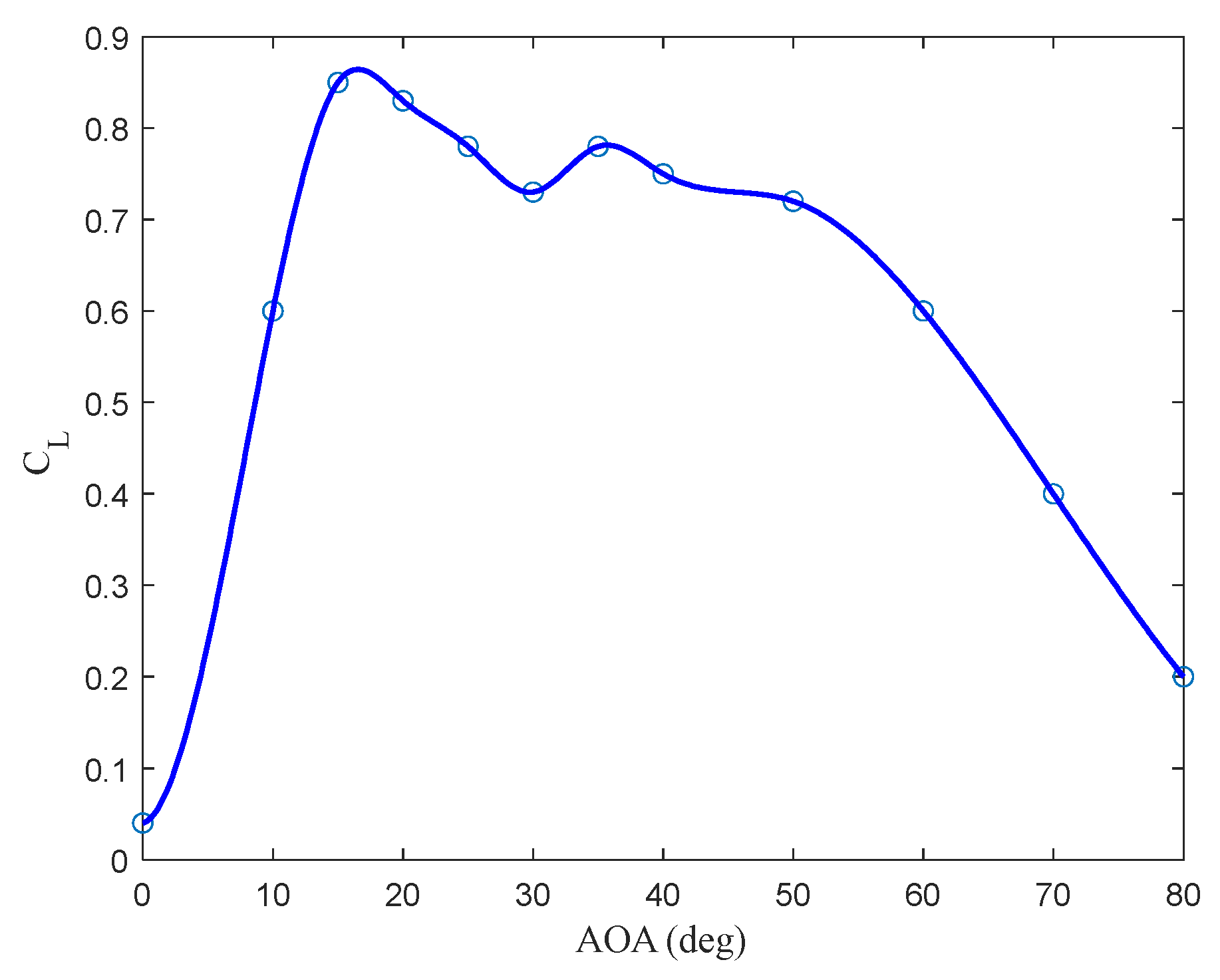
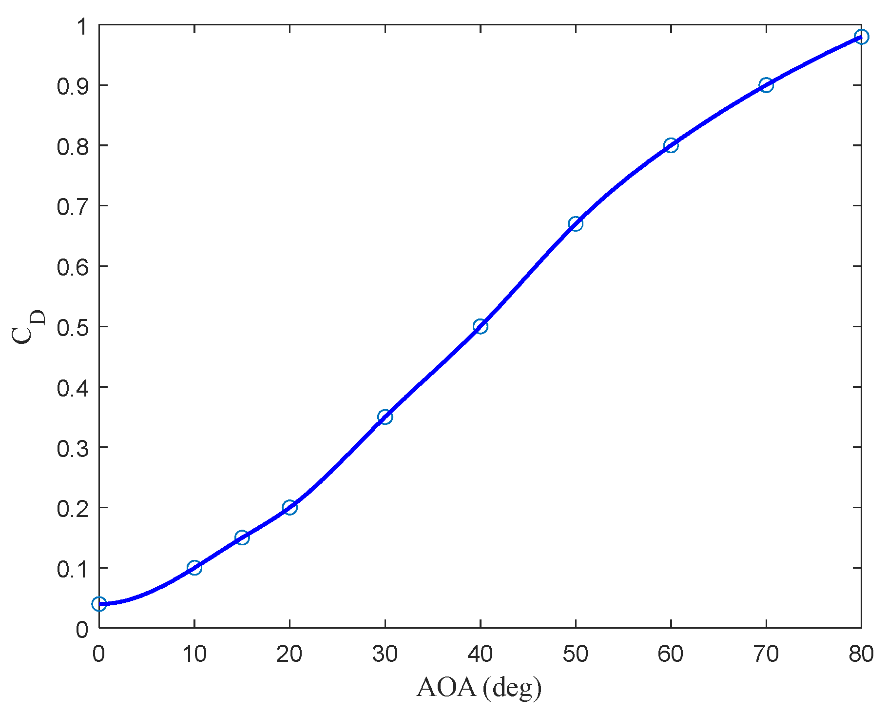
In this context, $F_D^i$ and $F_L^i$ represent the drag and lift forces generated by each wing, respectively, and can be determined from

$$\left[\begin{array}{c}{F}_D^i\\ 0\\ F_L^i\end{array}\right]=\mathit{R}\left({\theta }_i-{\alpha }_i\right)\left[\begin{array}{c}-{\displaystyle \frac{1}{2}}{C}_D\left({\alpha }_i\right)\rho A{v}^2\\ 0\\ -{\displaystyle \frac{1}{2}}{C}_L\left({\alpha }_i\right)\rho A{v}^2\end{array}\right]’$$

(10)

where ${\alpha }_i$ represents the wing’s effective angle of attack, $\rho$is the air density, $A$ denotes the wing area, and $v$ is the QTW’s velocity. $C_D$ and $C_L$ are the drag and lift coefficients, respectively.

Lastly, the gravitational force in the body frame is calculated as

$${\mathit{F}}_g=\left[\begin{array}{c}-\mathit{sin}(\theta )\\ \mathit{sin}(\varphi \left)\mathit{cos}(\theta \right)\\ \mathit{cos}(\varphi \left)\mathit{cos}(\theta \right)\end{array}\right]mg.$$

(11)

The total moment ${\mathit{M}}_t$ comprises the thrust moment ${\mathit{M}}_{th}$, the aerodynamic moment ${\mathit{M}}_{aero}$, and the gyroscopic moment of propellers ${\mathit{M}}_{gyro}$:

$${\mathit{M}}_t={\mathit{M}}_{th}+{\mathit{M}}_{aero}+{\mathit{M}}_{gyro}.$$

(12)

Moments ${\mathit{M}}_{th}$, ${\mathit{M}}_{aero}$, and ${\mathit{M}}_{gyro}$ can be calculated using the following three Equations (13)–(15), respectively:

$${\mathit{M}}_{th}=l_s\left[\begin{array}{cccc}\begin{array}{c}\mathrm{S}({\theta }_1)-{\displaystyle \frac{{\lambda }_1}{l_s}}\mathrm{C}({\theta }_1)\\ {\displaystyle \frac{l_l}{l_s}}\mathrm{S}({\theta }_1)\\ \mathrm{C}({\theta }_1)+{\displaystyle \frac{{\lambda }_1}{l_s}}\mathrm{S}({\theta }_1)\end{array}& \begin{array}{c}-\mathrm{S}({\theta }_2)-{\displaystyle \frac{{\lambda }_2}{l_s}}\mathrm{C}({\theta }_2)\\ {\displaystyle \frac{l_l}{l_s}}\mathrm{S}({\theta }_2)\\ -\mathrm{C}({\theta }_1)+{\displaystyle \frac{{\lambda }_2}{l_s}}\mathrm{S}({\theta }_2)\end{array}& \begin{array}{c}\mathrm{S}({\theta }_3)-{\displaystyle \frac{{\lambda }_3}{l_s}}\mathrm{C}({\theta }_3)\\ -{\displaystyle \frac{l_l}{l_s}}\mathrm{S}({\theta }_3)\\ \mathrm{C}({\theta }_3)+{\displaystyle \frac{{\lambda }_3}{l_s}}\mathrm{S}({\theta }_3)\end{array}& \begin{array}{c}-\mathrm{S}({\theta }_4)-{\displaystyle \frac{{\lambda }_4}{l_s}}\mathrm{C}({\theta }_4)\\ -{\displaystyle \frac{l_l}{l_s}}\mathrm{S}({\theta }_4)\\ -\mathrm{C}({\theta }_4)+{\displaystyle \frac{{\lambda }_4}{l_s}}\mathrm{S}({\theta }_4)\end{array}\end{array}\right]\left[\begin{array}{c}k{\omega }_1^2\\ k{\omega }_2^2\\ k{\omega }_3^2\\ k{\omega }_4^2\end{array}\right],$$

(13)

$${\mathit{M}}_{aero}=\left[\begin{array}{c}{l}_s(F_L^1-F_L^2+F_L^3-F_L^4)\\ l_l(F_L^1+F_L^2-F_L^3-F_L^4)\\ l_s(-F_D^1+F_D^2-F_D^3+F_D^4)\end{array}\right],$$

(14)

$${\mathit{M}}_{gyro}={\sum }_{i=1}^4{\mathit{J}}_{prop}\left[{\eta }_i{\Omega }_b\times \left[\begin{array}{c}\mathit{cos}({\theta }_i)\\ 0\\ -\mathit{sin}({\theta }_i)\end{array}\right]{\omega }_i\right],$$

(15)

where ${\mathit{l}}_l$ and ${\mathit{l}}_s$ represent the longitudinal and spanwise distances between the rotors and the center of gravity (CG), respectively; $\lambda$ denotes the torque-to-thrust ratio; and $\mathit{\eta }$ is a factor with a value of 1 for motors 1 and 4, and −1 for motors 2 and 3. Also, ${\mathit{J}}_{prop}$ denotes the prop moment of inertia.

2.4. Simplifying Dynamic Model

To simplify the motor forces (8) and moments (13), they can be rewritten in the form presented in (16), assuming that the front wings share the same tilt angle, ${\mathit{\theta }}_f$, and the rear wings share a similar tilt angle, ${\mathit{\theta }}_r$.

$$\left[\begin{array}{c}{\mathit{R}}_{wb}{\mathit{F}}_{th}\\ {\mathit{M}}_{th}\end{array}\right]=\left[\begin{array}{c}\left(\mathit{cos}(\varphi \right)\mathit{sin}(\theta \left)\mathit{cos}(\psi \right)+\mathit{sin}(\varphi \left)\mathit{sin}(\psi \right))U_V+\mathit{cos}(\psi )\mathit{cos}(\theta )U_H\\ \left(\mathit{cos}(\varphi \right)\mathit{sin}(\theta \left)\mathit{sin}(\psi \right)-\mathit{sin}(\varphi \left)\mathit{cos}(\psi \right))U_V+\mathit{sin}(\psi )\mathit{cos}(\theta )U_H\\ \mathit{cos}(\varphi \left)\mathit{cos}(\theta \right)U_V-\mathit{sin}(\theta )U_H\\ \begin{array}{c}\left(l_s\mathit{sin}({\theta }_f\right)-\lambda \mathit{cos}({\theta }_f\left)\right)U_{f_{dif}}+\left(l_s\mathit{sin}({\theta }_r\right)+\lambda \mathit{cos}({\theta }_r\left)\right)U_{r_{dif}}\\ \left[U_{f_{sum}}\mathit{sin}({\theta }_f)-U_{r_{sum}}\mathit{sin}({\theta }_r)\right]l_l\\ \left(l_s\mathit{cos}({\theta }_f\right)+\lambda \mathit{sin}({\theta }_f\left)\right)U_{f_{dif}}+\left(l_s\mathit{cos}({\theta }_r\right)-\lambda \mathit{sin}({\theta }_r\left)\right)U_{r_{dif}}\end{array}\end{array}\right]’$$

(16)

where

$$\begin{gathered} U_{f_{dif}}=k\left({\omega }_1^2-{\omega }_2^2\right), \\ {U}_{r_{dif}}=k\left({\omega }_3^2-{\omega }_4^2\right), \\ {U}_{f_{sum}}=k\left({\omega }_1^2+{\omega }_2^2\right), \\ {U}_{r_{sum}}=k\left({\omega }_3^2+{\omega }_4^2\right), \\ \hspace{1em}\hspace{1em}\hspace{1em}\hspace{1em}\hspace{1em}\hspace{1em}{U}_V=-\mathit{sin}({\theta }_f)U_{f_{sum}}-\mathit{sin}({\theta }_r)U_{r_{sum}}, \\ \hspace{1em}\hspace{1em}\hspace{1em}\hspace{1em}\hspace{1em}\hspace{1em}{U}_H=\mathit{cos}({\theta }_f)U_{f_{sum}}+\mathit{cos}({\theta }_r)U_{r_{sum}}. \end{gathered}$$

If we assume that all wings have the same tilt angle, ${\theta }_f={\theta }_r$, then the above equations can be further simplified as follows:

$$\left[\begin{array}{c}{\mathit{R}}_{wb}{\mathit{F}}_{th}\\ {\mathit{M}}_{th}\end{array}\right]=\left[\begin{array}{c}\left(\mathit{cos}(\psi \right)\mathit{cos}(\theta \left)\mathit{cos}({\theta }_f\right)-\left(\mathit{cos}(\varphi \right)\mathit{sin}(\theta \left)\mathit{cos}(\psi \right)+\mathit{sin}(\varphi \left)\mathit{sin}(\psi \right)\left)\mathit{sin}({\theta }_f\right))U_1\\ \left(\mathit{sin}(\psi \right)\mathit{cos}(\theta \left)\mathit{cos}({\theta }_f\right)-\left(\mathit{cos}(\varphi \right)\mathit{sin}(\theta \left)\mathit{sin}(\psi \right)-\mathit{sin}(\varphi \left)\mathit{cos}(\psi \right)\left)\mathit{sin}({\theta }_f\right))U_1\\ (-\mathit{sin}(\theta )\mathit{cos}({\theta }_f)-\mathit{cos}(\varphi )\mathit{cos}(\theta \left)\mathit{sin}({\theta }_f\right))U_1\\ \begin{array}{c}\mathit{sin}({\theta }_f)U_2-\mathit{cos}({\theta }_f)U_4\\ \mathit{sin}({\theta }_f)U_3\\ \mathit{cos}({\theta }_f)U_2+\mathit{sin}({\theta }_f)U_4\end{array}\end{array}\right],$$

(17)

where

$$\begin{gathered} U_1=k{({\omega }_1^2+{\omega }_2^2+{\omega }_3^2+{\omega }_4^2)}^{\prime } \\ {U}_2=k{l}_s{({\omega }_1^2-{\omega }_2^2+{\omega }_3^2-{\omega }_4^2)}^{\prime } \\ {U}_3=k{l}_l{({\omega }_1^2+{\omega }_2^2-{\omega }_3^2-{\omega }_4^2)}^{\prime } \\ {U}_4=k\lambda {({\omega }_1^2-{\omega }_2^2-{\omega }_3^2+{\omega }_4^2)}^{\prime } \end{gathered}$$

Similarly, the total aerodynamic force (9) and moment (14) generated by the wings can be expressed in the following form:

$$\left[\begin{array}{c}{\mathit{R}}_{wb}{\mathit{F}}_{aero}\\ {\mathit{M}}_{aero}\end{array}\right]=\left[\begin{array}{c}{W}_x\\ W_y\\ \begin{array}{c}{W}_z\\ 0\\ \begin{array}{c}{W}_t\\ 0\end{array}\end{array}\end{array}\right]\left[\begin{array}{c}{\mathit{R}}_{wb}\left[\begin{array}{c}2(F_D^f+F_D^r)\\ 0\\ 2(F_L^f+F_L^r)\end{array}\right]\\ \begin{array}{c}0\\ \begin{array}{c}2l_l(F_L^f-F_L^r)\\ 0\end{array}\end{array}\end{array}\right],$$

(18)

assuming that the front wings share the same tilt angle and the rear wings also share a common tilt angle, where superscript $f$ denotes the front wings, while superscript $r$ represents the rear wings. Also, $W_x$, $W_y$, and $W_z$ represent the aerodynamic forces along each body axis, and $W_t$ denotes the aerodynamic pitch moment. Since this work focuses on longitudinal motion, the roll and yaw moments are excluded from consideration.

Finally, assuming identical tilt angles for all wings and utilizing the simplified forces and moments derived above, the nonlinear dynamic form of the 6-DOF equations of motion for the QTW can be expanded as

$$\begin{gathered} \ddot{X}={\displaystyle \frac{1}{m}}{\left[(\mathit{cos}\psi \mathit{cos}\theta \mathit{cos}{\theta }_f-(\mathit{cos}\varphi \mathit{sin}\theta \mathit{cos}\psi +\mathit{sin}\varphi \mathit{sin}\psi \left)\mathit{sin}{\theta }_f\right)U_1+W_x\right]}^{\prime } \\ \ddot{Y}={\displaystyle \frac{1}{m}}{\left[(\mathit{sin}\psi \mathit{cos}\theta \mathit{cos}{\theta }_f-(\mathit{cos}\varphi \mathit{sin}\theta \mathit{sin}\psi -\mathit{sin}\varphi \mathit{cos}\psi \left)\mathit{sin}{\theta }_f\right)U_1+W_y\right]}^{\prime } \\ \ddot{Z}={\displaystyle \frac{1}{m}}{\left[(-\mathit{sin}\theta \mathit{cos}{\theta }_f-\mathit{cos}\varphi \mathit{cos}\theta \mathit{sin}{\theta }_f)U_1+mg+W_z\right]}^{\mathrm{\prime }} \\ \dot{p}={\displaystyle \frac{1}{I_{xx}}}[\mathit{sin}{\theta }_f{U}_2-\mathit{cos}{\theta }_f{U}_4]+{\displaystyle \frac{I_{yy}-I_{zz}}{I_{xx}}}qr-{\displaystyle \frac{J_{prop}}{I_{xx}}}q{\omega }_p{\mathit{sin}{\theta }_f}^{\prime } \\ \dot{q}={\displaystyle \frac{\mathit{sin}{\theta }_f{U}_3}{I_{yy}}}+{\displaystyle \frac{I_{zz}-I_{xx}}{I_{yy}}}pr+{\displaystyle \frac{J_{prop}}{I_{yy}}}(p\mathit{sin}{\theta }_f+r\mathit{cos}{\theta }_f){\omega }_p+{{\displaystyle \frac{W_t}{I_{yy}}}}^{\prime } \\ \dot{r}={\displaystyle \frac{1}{I_{zz}}}\left[\mathit{cos}{\theta }_f{U}_2+\mathit{sin}{\theta }_f{U}_4\right]+{\displaystyle \frac{I_{xx}-I_{yy}}{I_{zz}}}pq-{\displaystyle \frac{J_{prop}}{I_{zz}}}q{\omega }_p\mathit{cos}{\theta }_f. \end{gathered}$$

(19)

where ${\omega }_p={\omega }_1-{\omega }_2-{\omega }_3+{\omega }_4$.

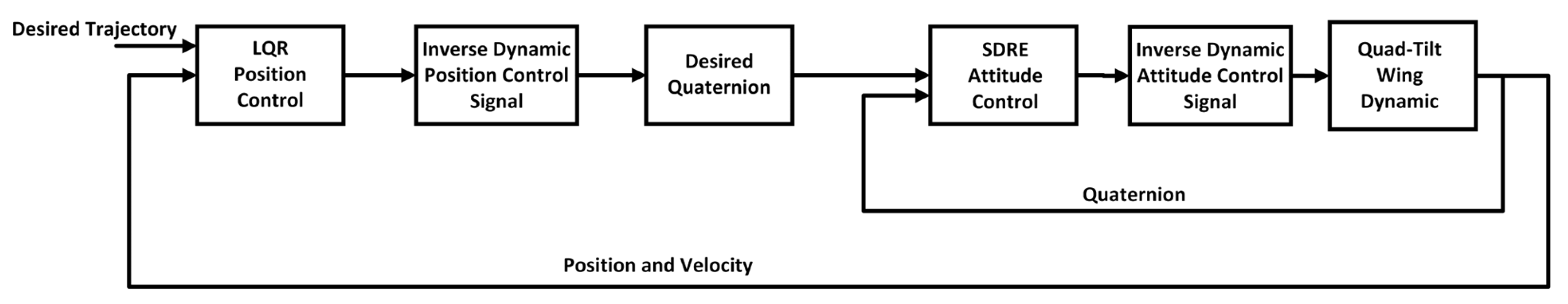
3. Optimal Control Design

This section describes the design of the nonlinear optimal control approach for the QTW vehicle. Figure 4 illustrates the control block diagram. As shown, the outer loop performs position–velocity control, utilizing a Linear Quadratic Regulator (LQR) combined with an inverse dynamics method to track the desired trajectory. The resulting position control signal is used to compute the desired quaternion parameters, which are then fed into the inner attitude control loop.

In the attitude control loop, a State-Dependent Riccati Equation (SDRE) method is employed to generate the optimal control signals, which are further processed using an inverse dynamics method to ensure the accurate tracking of the outer-loop commands.

Quaternion parameters are used in the attitude control loop instead of Euler angles to simplify the analytical solution for the SDRE and eliminate the need to solve the Riccati equation at each sample time. This approach facilitates the real-time control of the system. Furthermore, using quaternion parameters avoids the singularity issues associated with Euler angles, ensuring a robust and efficient control framework.

The SDRE method is similar to the LQR approach, with the key difference being that the linear quadratic equations in SDRE are not constant, but rather they vary and are state-dependent. This section first introduces the optimal control approach for state-space equations, followed by the design of the control loops.

3.1. Optimal Control Design for State-Space Equations

Assume an infinite-horizon regulation control problem for a system described by the state-space equations in Equation (20). It is further assumed that the system is controllable and affine in the input. The objective of the control problem is to determine the optimal regulator control signal that minimizes the cost function defined in Equation (21):

$$\dot{\mathit{x}}=\mathit{A}\left(\mathit{x}\right)\mathit{x}+\mathit{B}\left(\mathit{x}\right)\mathit{u},$$

(20)

$$J={\displaystyle \frac{1}{2}}{\int }_0^{\infty }\left({\mathit{x}}^T\mathit{Q}\left(\mathit{x}\right)\mathit{x}+{\mathit{u}}^T\mathit{R}\left(\mathit{x}\right)\mathit{u}\right)dt,$$

(21)

where $\mathit{Q}\left(\mathit{x}\right)$ and $\mathit{R}\left(\mathit{x}\right)$ are positive definite state- and control-weighting matrices, respectively. In (21), if the system is linear, then the problem corresponds to an LQR, where $\mathit{A}$ and $\mathit{B}$ are constant matrices. If the system is nonlinear, then $\mathit{A}\left(\mathit{x}\right)$ and $\mathit{B}\left(\mathit{x}\right)$ become state-dependent functions, and the problem is addressed using the SDRE control approach.

The solution to the defined optimal control problem is provided in (22), where $\mathit{P}\left(\mathit{x}\right)$ is determined as the solution to the Riccati equation presented in (23). Additionally, $\mathit{P}\left(\mathit{x}\right)$ is a symmetric and positive definite matrix.

$$\mathit{u}\left(\mathit{x}\right)=-\mathit{K}\left(\mathit{x}\right)\mathit{x}=-{\mathit{R}}^{-1}\left(\mathit{x}\right){\mathit{B}}^T\left(\mathit{x}\right)\mathit{P}\left(\mathit{x}\right)\mathit{x},$$

(22)

$${\mathit{A}}^T\left(\mathit{x}\right)\mathit{P}\left(\mathit{x}\right)+\mathit{P}\left(\mathit{x}\right)\mathit{A}\left(\mathit{x}\right)+\mathit{Q}\left(\mathit{x}\right)-\mathit{P}\left(\mathit{x}\right)\mathit{B}\left(\mathit{x}\right){\mathit{R}}^{-1}\left(\mathit{x}\right){\mathit{B}}^T\left(\mathit{x}\right)\mathit{P}\left(\mathit{x}\right)=0.$$

(23)

3.2. Outer Loop, Trajectory Control Design

This loop is designed using the LQR approach. To achieve this, the first three nonlinear equations in (19) are simplified into the following form:

$$\begin{gathered} {\ddot{\mathit{P}}}_W={\dot{\mathit{V}}}_w=\mathcal{z}, \\ {\mathcal{z}}_x=\ddot{X}={\displaystyle \frac{1}{m}}\left[(\mathit{cos}\psi \mathit{cos}\theta \mathit{cos}{\theta }_f-(\mathit{cos}\varphi \mathit{sin}\theta \mathit{cos}\psi +\mathit{sin}\varphi \mathit{sin}\psi \left)\mathit{sin}{\theta }_f\right)U_1+W_x\right], \\ {\mathcal{z}}_y=\ddot{Y}={\displaystyle \frac{1}{m}}\left[(\mathit{sin}\psi \mathit{cos}\theta \mathit{cos}{\theta }_f-(\mathit{cos}\varphi \mathit{sin}\theta \mathit{sin}\psi -\mathit{sin}\varphi \mathit{cos}\psi \left)\mathit{sin}{\theta }_f\right)U_1+W_y\right], \\ {\mathcal{z}}_z=\ddot{Z}={\displaystyle \frac{1}{m}}\left[(-\mathit{sin}\theta \mathit{cos}{\theta }_f-\mathit{cos}\varphi \mathit{cos}\theta \mathit{sin}{\theta }_f)U_1+mg+W_z\right], \end{gathered}$$

(24)

Unlike traditional linearization around an equilibrium point, this reformulation expresses the system dynamics in a structured second-order form, allowing the application of the LQR for optimal trajectory tracking. The actual control inputs are then computed using the full nonlinear system dynamics, ensuring that the approach remains valid beyond small perturbations.

By leveraging the complete nonlinear model for control input computation, this method provides a broader applicability compared to standard linearized approaches. A similar control strategy—combining reformulated equations, the LQR, and inverse dynamics—was successfully applied in another work on the dynamic control of an aerial manipulation system [31]. In that study, the approach demonstrated comparable performance to an adaptive sliding mode controller, further validating its effectiveness in handling highly nonlinear dynamic systems.

The corresponding constant state-space equations are formulated as

$$\begin{gathered} \mathit{x}=\left[\begin{array}{c}{\mathit{V}}_W\\ {\mathit{P}}_W\end{array}\right],\left[\begin{array}{c}{\dot{\mathit{V}}}_W\\ {\dot{\mathit{P}}}_W\end{array}\right]=\left[\begin{array}{cc}{\mathbf{0}}_3& {\mathbf{0}}_3\\ {\mathit{I}}_3& {\mathbf{0}}_3\end{array}\right]\left[\begin{array}{c}{\mathit{V}}_W\\ {\mathit{P}}_W\end{array}\right]+\left[\begin{array}{c}{\mathit{I}}_3\\ {\mathbf{0}}_3\end{array}\right]\mathcal{z}, \\ \mathit{A}=\left[\begin{array}{cc}{\mathbf{0}}_3& {\mathbf{0}}_3\\ {\mathit{I}}_3& {\mathbf{0}}_3\end{array}\right], \mathit{B}=\left[\begin{array}{c}{\mathit{I}}_3\\ {\mathbf{0}}_3\end{array}\right], \end{gathered}$$

(25)

where $\mathcal{z}={\left[{\mathcal{z}}_x,{\mathcal{z}}_y,{\mathcal{z}}_z\right]}^T$ represents the new position control signal, which is derived using the LQR method.

3.2.1. Outer Loop Controllability

To assess the controllability of the position state-space equations in Equation (25), the controllability matrix ${\widehat{\mathit{C}}}_{\mathit{A},\mathit{B} }$ is constructed as

$${\widehat{\mathit{C}}}_{\mathit{A},\mathit{B} }=\left[\begin{array}{cccc}\mathit{B}& \mathit{A}\mathit{B}& \cdots & {\mathit{A}}^5\mathit{B}\end{array}\right],$$

(26)

It is noteworthy that ${\mathit{A}}^{\mathit{K}}$ for $\mathit{k}\ge \mathbf{2}$ is zero. As a result, it is sufficient to evaluate the controllability of the simplified matrix, ${\widehat{\mathit{C}}}_{\mathit{A},\mathit{B}}$:

$${\widehat{\mathit{C}}}_{\mathit{A},\mathit{B}}=\left[\mathit{B}\mathit{}\mathit{}\mathit{}\hspace{1em}\mathit{A}\mathit{B}\right]=\left[\begin{array}{cc}{\mathit{I}}_3& {\mathbf{0}}_3\\ {\mathbf{0}}_3& {\mathit{I}}_3\end{array}\right].$$

(27)

Since ${\widehat{\mathit{C}}}_{\mathit{A},\mathit{B}}$ is a square matrix, it is full rank and therefore controllable if and only if its determinant is nonzero. As $\left|{\widehat{\mathit{C}}}_{\mathit{A},\mathit{B}}\right|=1$, the system is confirmed to be controllable.

3.2.2. LQR Analytical Solution

To solve the Riccati equation in Equation (23), the weighting matrices $\mathit{Q}$ and $\mathit{R}$ are defined as positive:

$$\begin{gathered} \mathit{Q}=\left[\begin{array}{cc}{\mathit{Q}}_1& {\mathbf{0}}_3\\ {\mathbf{0}}_3& {\mathit{Q}}_2\end{array}\right], \\ {\mathit{Q}}_1=diag\left(q_{1i}^2\right) {\mathit{I}}_3, \\ {\mathit{Q}}_2=diag\left(q_{2i}^2\right) {\mathit{I}}_3, \end{gathered}$$

(28)

$$\mathit{R}=diag\left(r_i^2\right){\mathit{I}}_3, i=\mathrm{1,2},3,$$

(29)

where $q_{1i}$, $q_{2i}$, and $r_i$ are positive real number.

The solution to the Riccati equation $\mathit{P}$ can be written as

$$\mathit{P}=\left[\begin{array}{cc}{\mathit{P}}_1& {\mathit{P}}_2\\ {\mathit{P}}_3& {\mathit{P}}_4\end{array}\right],$$

(30)

where ${\mathit{P}}_1$ to ${\mathit{P}}_4$ are square matrices of size 3. Among these, ${\mathit{P}}_1$ and ${\mathit{P}}_4$ are symmetric and positive definite. While ${\mathit{P}}_2$ and ${\mathit{P}}_3$ are not necessarily positive definite, they satisfy the relationship ${\mathit{P}}_3={\mathit{P}}_2^{\mathit{T}}$.

By substituting Equations (25) and (28)–(30) into Equation (23) and solving for $\mathit{P}$, the following equations can be obtained:

$${\mathit{P}}_2^T+{\mathit{P}}_2-{\mathit{P}}_1{\mathit{R}}^{-1}{\mathit{P}}_1+{\mathit{Q}}_1=\mathbf{0},$$

(31)

$${\mathit{P}}_4-{\mathit{P}}_1{\mathit{R}}^{-1}{\mathit{P}}_2=\mathbf{0},$$

(32)

$${\mathit{P}}_4-{\mathit{P}}_2^T{\mathit{R}}^{-1}{\mathit{P}}_1=\mathbf{0},$$

(33)

$$-{\mathit{P}}_2^T{\mathit{R}}^{-1}{\mathit{P}}_2+{\mathit{Q}}_2=\mathbf{0}.$$

(34)

With Equation (22), the position control signal $\mathit{Z}$ is calculated:

$$\mathcal{z}=-{\mathit{R}}^{-1}({\mathit{P}}_1{\mathit{V}}_W+{\mathit{P}}_2{\mathit{P}}_W),$$

(35)

Therefore, it is required to find only ${\mathit{P}}_1$ and ${\mathit{P}}_2$. To determine ${\mathit{P}}_2$, Equation (34) is reformulated

$${\mathit{P}}_2^T\sqrt{{\mathit{R}}^{-1}}\sqrt{{\mathit{R}}^{-1}}{\mathit{P}}_2={(\mathit{P}}_2^T\sqrt{{\mathit{R}}^{-1}}{\left)\right({\mathit{P}}_2^T\sqrt{{\mathit{R}}^{-1}})}^T=\sqrt{{\mathit{Q}}_2}\sqrt{{\mathit{Q}}_2}.$$

(36)

which leads to the solution for ${\mathit{P}}_2$ as expressed by

$${\mathit{P}}_2={\mathit{P}}_2^T=\sqrt{{\mathit{Q}}_2}\sqrt{\mathit{R}},$$

(37)

This solution is possible because $\mathit{Q}$ and $\mathit{R}$ are diagonal matrices. With ${\mathit{P}}_2$ determined, ${\mathit{P}}_1$ can be obtained by rewriting Equation (31) into the following form:

$$2\sqrt{{\mathit{Q}}_2}\sqrt{\mathit{R}}+{\mathit{Q}}_1={\mathit{P}}_1{\mathit{R}}^{-1}{\mathit{P}}_1,$$

(38)

This leads to the solution that is expressed as

$${\mathit{P}}_1=\sqrt{\mathit{R}}\sqrt{2\sqrt{{\mathit{Q}}_2}\sqrt{\mathit{R}}+{\mathit{Q}}_1},$$

(39)

3.2.3. Outer Loop Stability Assessment

From Equations (24) and (35), the closed-loop position equations can be simplified as

$$\begin{gathered} {\dot{\mathit{P}}}_w={\mathit{V}}_w, \\ {\dot{\mathit{V}}}_w=-{\mathit{R}}^{-1}({\mathit{P}}_1{\mathit{V}}_W+{\mathit{P}}_2{\mathit{P}}_W). \end{gathered}$$

(40)

To analyze the stability of the closed-loop system expressed in Equation (40), the following Lyapunov function [32], which is radially bounded ($\underset{V\to \pm \infty }{\lim }L=\infty , \underset{P\to \pm \infty }{\lim }L=\infty$) and positive definite, is considered:

$$L={\displaystyle \frac{1}{2}}{{\mathit{V}}_w}^T{\mathit{P}}_1^{-1}\mathit{R}{\mathit{V}}_w+{\displaystyle \frac{1}{2}}{{\mathit{P}}_W}^T{\mathit{P}}_1^{-1}{\mathit{P}}_2{\mathit{P}}_W,$$

The derivative of the proposed Lyapunov function is given as $\dot{L}=-{{\mathit{V}}_w}^T{\mathit{V}}_w$, which is negative definite. This confirms the global stability of the designed LQR controller.

3.2.4. Outer Loop Stability Improvement

In this section, the control signal in (35) is modified to achieve exponential stability, which offers a guaranteed convergence rate. This ensures that the inner control loop operates at a faster timescale than the outer loop, maintaining hierarchical stability and improving overall controller efficiency. Compared to asymptotic stability, exponential stability provides a faster decay of errors, enhancing response time, robustness to disturbances, and predictability in control performance.

The modified control position signal is presented as

$$\mathcal{z}=-{\mathit{R}}^{-1}\left({\mathit{P}}_1{\mathit{V}}_W+{\mathit{P}}_2{\mathit{P}}_W\right)-\mathit{K}{\mathit{V}}_w-{\mathit{R}}^{-1}{\mathit{P}}_1\mathit{K}{\mathit{P}}_W,$$

where $\mathit{K}$ is a positive definite diagonal matrix. The stability of the enhanced position control signal is established using the following Lyapunov candidate function [32]:

$$L={\displaystyle \frac{1}{2}}{\left({\mathit{V}}_w+\mathit{K}{\mathit{P}}_W\right)}^T{\mathit{P}}_1^{-1}\mathit{R}\left({\mathit{V}}_w+\mathit{K}{\mathit{P}}_W\right)+{\displaystyle \frac{1}{2}}{{\mathit{P}}_W}^T{\mathit{P}}_1^{-1}{\mathit{P}}_2{\mathit{P}}_W.$$

The minimum convergence rate of the position controller is given by the following [32]:

$$\alpha ={\displaystyle \frac{min\left\{1,{\lambda }_{min}\left(\mathit{K}{\mathit{P}}_1^{-1}{\mathit{P}}_2\right)\right\}}{max\left\{\frac{{\lambda }_{max}\left({\mathit{P}}_1^{-1}\mathit{R}\right)}{2},\frac{{\lambda }_{max}\left({\mathit{P}}_1^{-1}{\mathit{P}}_2\right)}{2}\right\}}}$$

3.2.5. Desired Signal for Inner Loop

With the position control signal calculated with the LQR, $\mathcal{z}$, Equation (24) can be reformulated as

$$\begin{gathered} m{\mathcal{z}}_x-W_X=\left(\mathit{cos}\psi \mathit{cos}\theta \mathit{cos}{\theta }_f-\left(\mathit{cos}\varphi \mathit{sin}\theta \mathit{cos}\psi +\mathit{sin}\varphi \mathit{sin}\psi \right)\mathit{sin}{\theta }_f\right)U_1, \\ m{\mathcal{z}}_y-W_Y=\left(\mathit{sin}\psi \mathit{cos}\theta \mathit{cos}{\theta }_f-\left(\mathit{cos}\varphi \mathit{sin}\theta \mathit{sin}\psi -\mathit{sin}\varphi \mathit{cos}\psi \right)\mathit{sin}{\theta }_f\right)U_1, \\ m{\mathcal{z}}_z-W_Z-mg=\left(-\mathit{sin}\theta \mathit{cos}{\theta }_f-\mathit{cos}\varphi \mathit{cos}\theta \mathit{sin}{\theta }_f\right)U_1. \end{gathered}$$

(41)

Consequently, $U_1$ can be determined using

$$U_1=\sqrt{(m{\mathcal{z}}_x-W_X{)}^2+(m{\mathcal{z}}_y-W_Y{)}^2+(m{\mathcal{z}}_z-W_Z-mg{)}^2},$$

(42)

The desired roll and pitch angles can be calculated using

$$\begin{gathered} {\varphi }_d=a\mathit{sin}({\displaystyle \frac{-{\rho }_1}{U_1\mathit{sin}{\theta }_f}}), \\ {\theta }_d={\sin }^{-1}\left({\displaystyle \frac{-(m{\mathcal{z}}_z-W_Z-mg)U_1\mathit{cos}{\theta }_f-U_1{\rho }_2\mathit{sin}{\theta }_f\mathit{cos}{\varphi }_d}{{\rho }_2^2+(m{\mathcal{z}}_z-W_Z-mg{)}^2}}\right), \end{gathered}$$

(43)

where ${\rho }_1$ and ${\rho }_2$ are defind as

$$\begin{gathered} {\rho }_1=\left(m{\mathcal{z}}_x-W_X\right)\mathit{sin}{\psi }_d-\left(m{\mathcal{z}}_y-W_Y\right)\mathit{cos}{\psi }_d, \\ {\rho }_2=(m{\mathcal{z}}_x-W_X)\mathit{cos}{\psi }_d+(m{\mathcal{z}}_y-W_Y)\mathit{sin}{\psi }_d. \end{gathered}$$

It is assumed that the desired heading angle is known and is typically aligned with the desired trajectory. With all the desired Euler angles determined, the corresponding desired quaternion parameters can be calculated using

$$\begin{gathered} \eta =C({\displaystyle \frac{{\psi }_d}{2}})C({\displaystyle \frac{{\theta }_d}{2}})C({\displaystyle \frac{{\varphi }_d}{2}})+S({\displaystyle \frac{{\psi }_d}{2}})S({\displaystyle \frac{{\theta }_d}{2}})s({\displaystyle \frac{{\varphi }_d}{2}}) \\ {\mathrm{є}}_1=C({\displaystyle \frac{{\psi }_d}{2}})C({\displaystyle \frac{{\theta }_d}{2}})S({\displaystyle \frac{{\varphi }_d}{2}})-S({\displaystyle \frac{{\psi }_d}{2}})S({\displaystyle \frac{{\theta }_d}{2}})C({\displaystyle \frac{{\varphi }_d}{2}}) \\ {\mathrm{є}}_2=C({\displaystyle \frac{{\psi }_d}{2}})S({\displaystyle \frac{{\theta }_d}{2}})C({\displaystyle \frac{{\varphi }_d}{2}})+S({\displaystyle \frac{{\psi }_d}{2}})C({\displaystyle \frac{{\theta }_d}{2}})S({\displaystyle \frac{{\varphi }_d}{2}}) \\ \hspace{1em}\hspace{1em}\hspace{1em}{\mathrm{є}}_3=S\left({\displaystyle \frac{{\psi }_d}{2}}\right)C\left({\displaystyle \frac{{\theta }_d}{2}}\right)C\left({\displaystyle \frac{{\varphi }_d}{2}}\right)-C\left({\displaystyle \frac{{\psi }_d}{2}}\right)S\left({\displaystyle \frac{{\theta }_d}{2}}\right)S\left({\displaystyle \frac{{\varphi }_d}{2}}\right). \end{gathered}$$

(44)

where $\mathit{ϵ}={\left[\begin{array}{ccc}{ϵ}_1& {ϵ}_2& {ϵ}_3\end{array}\right]}^T$ denotes the vector part of the quaternion, and $\eta$ represents the scalar part.

3.3. Inner Loop, Attitude Control Design

In this section, the optimal inner control loop is designed using the SDRE approach by reformulating the nonlinear attitude equations in state-space form. This allows for stability assessment and the derivation of an analytical solution for the closed-loop system, followed by a stability analysis.

In recalling Equation (6) and the ${\dot{\mathit{\Omega }}}_b$ equation and introducing a new attitude control signal $\mathit{v}$, the attitude dynamics equation can be reformulated as

$${\dot{\mathit{\Omega }}}_b=\mathit{v}={\mathit{I}}_b^{-1}\left[{\mathit{M}}_t-{\mathit{\Omega }}_b\times \left({\mathit{I}}_b{\mathit{\Omega }}_b\right)\right].$$

(45)

In assuming that the QTW is controlled solely by its motors without any active aerodynamic surfaces and given $\mathit{v}$ from the optimal control signal, the total moment can be determined from

$${\mathit{M}}_t={\mathit{I}}_b\mathit{v}+{\mathit{\Omega }}_b\times \left({\mathit{I}}_b{\mathit{\Omega }}_b\right),$$

(46)

leading to the calculation of the required motor-generated moment:

$${\mathit{M}}_{th}={\mathit{M}}_t-{\mathit{M}}_{aero}-{\mathit{M}}_{gyro}.$$

(47)

Using Equation (17) for the same tilt angle, ${\mathit{M}}_{th}$ can be expressed as follows:

$${\mathit{M}}_{th}=\left[\begin{array}{ccc}\begin{array}{c}\mathit{sin}({\theta }_f)\\ 0\\ \mathit{cos}({\theta }_f)\end{array}& \begin{array}{c}0\\ \mathit{sin}({\theta }_f)\\ 0\end{array}& \begin{array}{c}-\mathit{cos}({\theta }_f)\\ 0\\ \mathit{sin}({\theta }_f)\end{array}\end{array}\right]\left[\begin{array}{c}{U}_2\\ U_3\\ U_4\end{array}\right].$$

The actual attitude control signal can be calculated using the following expression:

$$\left[\begin{array}{c}{U}_2\\ U_3\\ U_4\end{array}\right]={\left[\begin{array}{ccc}\begin{array}{c}\mathit{sin}({\theta }_f)\\ 0\\ \mathit{cos}({\theta }_f)\end{array}& \begin{array}{c}0\\ \mathit{sin}({\theta }_f)\\ 0\end{array}& \begin{array}{c}-\mathit{cos}({\theta }_f)\\ 0\\ \mathit{sin}({\theta }_f)\end{array}\end{array}\right]}^{-1}{\mathit{M}}_{th}.$$

(48)

To construct the state-space equations, an additional equation—the quaternion update equation, provided in the next section—is required.

3.3.1. Quaternion Update Equations and State-Space Attitude Equations

The quaternion update equations can be obtained as follows [33]:

$$\dot{ϵ}={\displaystyle \frac{1}{2}}\left(\eta {\mathit{\Omega }}_b+{\mathit{S}}_{ϵ}{\mathit{\Omega }}_b\right),$$

(49)

$$\dot{\eta }=-{\displaystyle \frac{1}{2}}{{\mathit{\Omega }}_b}^T\mathit{ϵ},$$

(50)

where

$${\mathit{S}}_{ϵ}=\left[\begin{array}{ccc}0& -{ϵ}_3& {ϵ}_2\\ {ϵ}_3& 0& -{ϵ}_1\\ -{ϵ}_2& {ϵ}_1& 0\end{array}\right].$$

It is important to note that quaternion parameters are not independent, as they are related according to the following equation:

$${\eta }^2+{\mathit{ϵ}}^T\mathit{ϵ}=1.$$

In utilizing Equations (45) and (49) and defining the state vector as $\mathit{x}=\left[\begin{array}{c}{\mathit{\Omega }}_b\\ \mathbf{є}\end{array}\right]$, the attitude equations can be expressed in state-space form as

$$\begin{gathered} \left[\begin{array}{c}{\dot{\mathit{\Omega }}}_b\\ \dot{\mathbf{є}}\end{array}\right]=\left[\begin{array}{cc}{\mathbf{0}}_3& {\mathbf{0}}_3\\ {\mathit{A}}_{\mathbf{є}}& {\mathbf{0}}_3\end{array}\right]\left[\begin{array}{c}{\mathit{\Omega }}_b\\ \mathbf{є}\end{array}\right]+\left[\begin{array}{c}{\mathit{I}}_3\\ {\mathbf{0}}_3\end{array}\right]\mathit{v}, \\ \mathit{A}=\left[\begin{array}{cc}{\mathbf{0}}_3& {\mathbf{0}}_3\\ {\mathit{A}}_{\mathbf{є}}& {\mathbf{0}}_3\end{array}\right],\mathit{B}=\left[\begin{array}{c}{\mathit{I}}_3\\ {\mathbf{0}}_3\end{array}\right], \end{gathered}$$

(51)

where

$${\mathit{A}}_{\mathbf{є}}={\displaystyle \frac{1}{2}}\left[\begin{array}{ccc}\eta & -{\mathrm{є}}_3& {\mathrm{є}}_2\\ {\mathrm{є}}_3& \eta & -{\mathrm{є}}_1\\ -{\mathrm{є}}_2& {\mathrm{є}}_1& \eta \end{array}\right].$$

3.3.2. Inner Loop Controllability

To evaluate the controllability of the attitude loop, the same equation as (26) is utilized, and only the controllability of the first two components needs to be assessed. Consequently, the modified controllability matrix is formulated as

$${\widehat{\mathit{C}}}_{\mathit{A},\mathit{B}}=\left[\mathit{B}\mathit{}\mathit{}\mathit{}\hspace{1em}\mathit{A}\mathit{B}\right]=\left[\begin{array}{cc}{\mathit{I}}_3& {\mathbf{0}}_3\\ {\mathbf{0}}_3& {\mathit{A}}_{ϵ}\end{array}\right].$$

(52)

The determinant of (52) is derived as $\left|{\widehat{\mathit{C}}}_{\mathit{A},\mathit{B}}\right|={\displaystyle \frac{1}{8}}\eta$. It is evident that if $\eta =0$, then the system is not point-to-point controllable; however, stability analysis in the subsequent sections will show that there are no instability issues, and the attitude control loop is indeed stable.

It is notable that, in this work, the controllability of the system is analyzed by considering the inner and outer control loops separately. Instead of linearizing around an operating point, we employ an inverse dynamics-based approach to transform the nonlinear system into a form suitable for state-space representation. This enables the application of optimal control techniques such as LQR for the outer loop and SDRE for the inner loop. The controllability of each resulting state-space formulation is verified to ensure that the system dynamics allow for proper control action within each loop.

It is important to note that proving controllability for each loop individually in its transformed state-space form does not automatically imply global controllability of the full nonlinear system. In nonlinear systems, a more rigorous assessment, such as Lie bracket analysis or differential geometric methods, is typically required to ensure full controllability. While our hierarchical control structure ensures that the inner loop operates at a faster time scale than the outer loop, leading to effective control execution, a complete nonlinear controllability analysis could be considered in future work to formally establish global controllability conditions.

3.3.3. SDRE Analytical Solution

In defining similar weighting matrices and a Riccati solution as in Equations (28)–(30) and solving the Riccati equation in Equation (23) for the attitude dynamics described in Equation (51), the following equations are derived, assuming for simplicity that $r_i=r$ and $q_{2i}=q_2$:

$${\mathit{A}}_{ϵ}^T{\mathit{P}}_2+{\mathit{P}}_2{\mathit{A}}_{ϵ}-{\displaystyle \frac{1}{r^2}}{\mathit{P}}_1^2+{\mathit{Q}}_1=\mathbf{0},$$

(53)

$${\mathit{A}}_{ϵ}^T{\mathit{P}}_4-{\displaystyle \frac{1}{r^2}}{\mathit{P}}_1{\mathit{P}}_2=\mathbf{0},$$

(54)

$${\mathit{P}}_4{\mathit{A}}_{ϵ}-{\displaystyle \frac{1}{r^2}}{\mathit{P}}_2^T{\mathit{P}}_1=\mathbf{0},$$

(55)

$$-{\displaystyle \frac{1}{r^2}}{\mathit{P}}_2^T{\mathit{P}}_2+{\mathit{Q}}_2=\mathbf{0}.$$

(56)

Using Equation (22) for the attitude equations in Equation (51), the optimal attitude control signal $\mathit{\nu }$ can be determined as follows

$$\mathit{\nu }=-{\displaystyle \frac{1}{r^2}}\left({\mathit{P}}_1{\mathit{\Omega }}_b+{\mathit{P}}_2\mathit{ϵ}\right).$$

(57)

The SDRE control signal, $\mathit{\nu }$, obtained in Equation (57), is used in Equation (46) to compute the total moment required for attitude control using the inverse dynamics approach. Then, using Equation (48), the control signal for the attitude is determined.

To find the SDRE control signal, it is required to calculate ${\mathit{P}}_1$ and ${\mathit{P}}_2$. ${\mathit{P}}_2$ can be calculated using Equation (56) as

$${\mathit{P}}_2=r{q}_2{\mathit{I}}_3.$$

(58)

To find ${\mathit{P}}_1$, Equation (53) can be rewritten as

$${\mathit{P}}_1^2=r^2\left({\mathit{A}}_{ϵ}^T{\mathit{P}}_2+{\mathit{P}}_2{\mathit{A}}_{ϵ}+{\mathit{Q}}_1\right).$$

(59)

Given that ${\mathit{P}}_1$ is positive definite, it can be determined using Singular Value Decomposition (SVD) as follows:

$${\mathit{P}}_1=diag\left(r\sqrt{q_{1i}^2+r{q}_2\eta }\right) ,i=\mathrm{1,2},3.$$

(60)

3.3.4. Inner Loop Stability Assessment

To analyze the stability of the system using Lyapunov’s method, the closed-loop attitude control equation can be formulated by combining Equations (45) and (57) as

$${\dot{\mathit{\Omega }}}_b==-{\displaystyle \frac{1}{r^2}}\left({\mathit{P}}_1{\mathit{\Omega }}_b+{\mathit{P}}_2\mathit{ϵ}\right),$$

(61)

The following Lyapanov function [32], which is positive definite and radially unbounded with respect to the ${\mathit{\Omega }}_b$, where ($\underset{{\mathit{\Omega }}_b\to \pm \mathit{\infty }}{\mathit{lim}}L=\mathit{\infty }$), is considered:

$$L={\displaystyle \frac{1}{2}}{r}^2{{\mathit{\Omega }}_b}^T{\mathit{P}}_2^{-1}{\mathit{\Omega }}_b+{\mathit{ϵ}}^T\mathit{ϵ}+{\left(1-\eta \right)}^2.$$

(62)

The time derivative of this Lyapunov function is calculated by

$$\dot{L}={-{\mathit{\Omega }}_b}^T{\mathit{P}}_2^{-1}{\mathit{P}}_1{\mathit{\Omega }}_b.$$

(63)

The detailed derivation of the Lyapunov function is presented in Appendix A. Since ${\mathit{P}}_2$ is both symmetric and positive definite, it can be concluded that

$$\left\{\begin{array}{c}\dot{L}<0 \forall {\mathit{\Omega }}_b\ne 0\\ \dot{L}=0 \forall {\mathit{\Omega }}_b=0\end{array}\right.$$

This demonstrates the stability of the attitude loop around the following equilibrium point:

$$\mathit{ϵ}=\mathbf{0},\mathit{}\eta =\pm 1.$$

The controllability issue is revisited to consider the worst-case scenario, in which both $\eta$ and ${\mathit{\Omega }}_b$ are zero. In this case, the Lyapunov function becomes $L={\mathit{ϵ}}^T\mathit{ϵ}+1>0 \forall {\mathit{\Omega }}_b,\eta =0$ and $\underset{t\to \infty }{\mathit{lim}}L=\infty$. Therefore, even in this scenario, the system remains stable.

3.3.5. Inner Loop Stability Improvement

Similarly to position control, adding terms to the attitude control signal in (57) enhances the inner loop stability from asymptotic to exponential stability. This modification ensures faster convergence and improved robustness. Based on this, the following enhanced control signal is proposed:

$$\mathit{\nu }=-{\displaystyle \frac{1}{r^2}}\left({\mathit{P}}_1{\mathit{\Omega }}_b+{\mathit{P}}_2\mathit{ϵ}\right)-{\displaystyle \frac{1}{r^2}}\left({\mathit{P}}_1\mathit{\Gamma }\mathit{ϵ}\right)-\mathit{\Gamma }\dot{\mathit{ϵ}}$$

where $\mathit{\Gamma }$ is a positive definite diagonal matrix. The exponential stability of the proposed attitude control signal is established using the following Lyapunov function:

$$L={\displaystyle \frac{1}{2}}{r}^2{\left({\mathit{\Omega }}_b+\mathit{\Gamma }\mathit{ϵ}\right)}^T{\mathit{P}}_2^{-1}\left({\mathit{\Omega }}_b+\mathit{\Gamma }\mathit{ϵ}\right)+{\mathit{ϵ}}^T\mathit{ϵ}+{\left(1-\eta \right)}^2$$

The minimum convergence rate can also be found as follows [32]:

$$\beta ={\displaystyle \frac{min\left\{{\lambda }_{min}\left(\mathit{\Gamma }\right),{\lambda }_{min}\left({\mathit{P}}_2^{-1}{\mathit{P}}_1\right)\right\}}{max\left\{2,\frac{{\lambda }_{max}\left({\mathit{P}}_2^{-1}\right)r^2}{2}\right\}}}$$

Therefore, to ensure a stable control loop and a faster inner loop, $\beta >\alpha$ must hold. To satisfy this condition, the $\mathit{Q}$ and $\mathit{R}$ matrix parameters for both loops should be defined such that the inner loop operates at a higher bandwidth than the outer loop, ensuring faster response and stability.

$${\displaystyle \frac{min\left\{{\lambda }_{min}\left(\mathit{\Gamma }\right),{\lambda }_{min}\left({\mathit{P}}_2^{-1}{\mathit{P}}_1\right)\right\}}{max\left\{2,\frac{{\lambda }_{max}\left({\mathit{P}}_2^{-1}\right)r^2}{2}\right\}}}\ge {\displaystyle \frac{min\left\{1,{\lambda }_{min}\left(\mathit{K}{\mathit{P}}_1^{-1}{\mathit{P}}_2\right)\right\}}{max\left\{\frac{{\lambda }_{max}\left({\mathit{P}}_1^{-1}\mathit{R}\right)}{2},\frac{{\lambda }_{max}\left({\mathit{P}}_1^{-1}{\mathit{P}}_2\right)}{2}\right\}}}$$

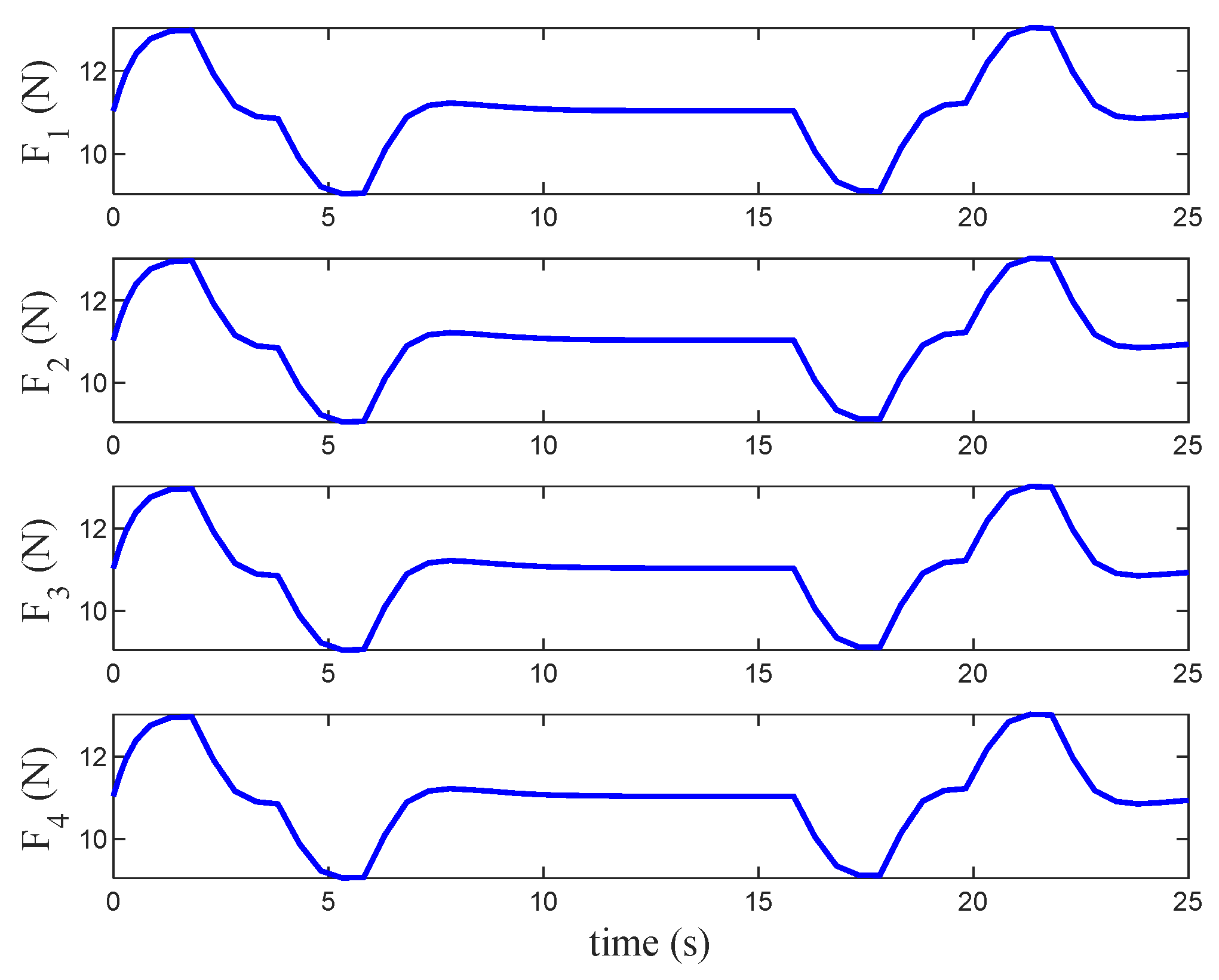
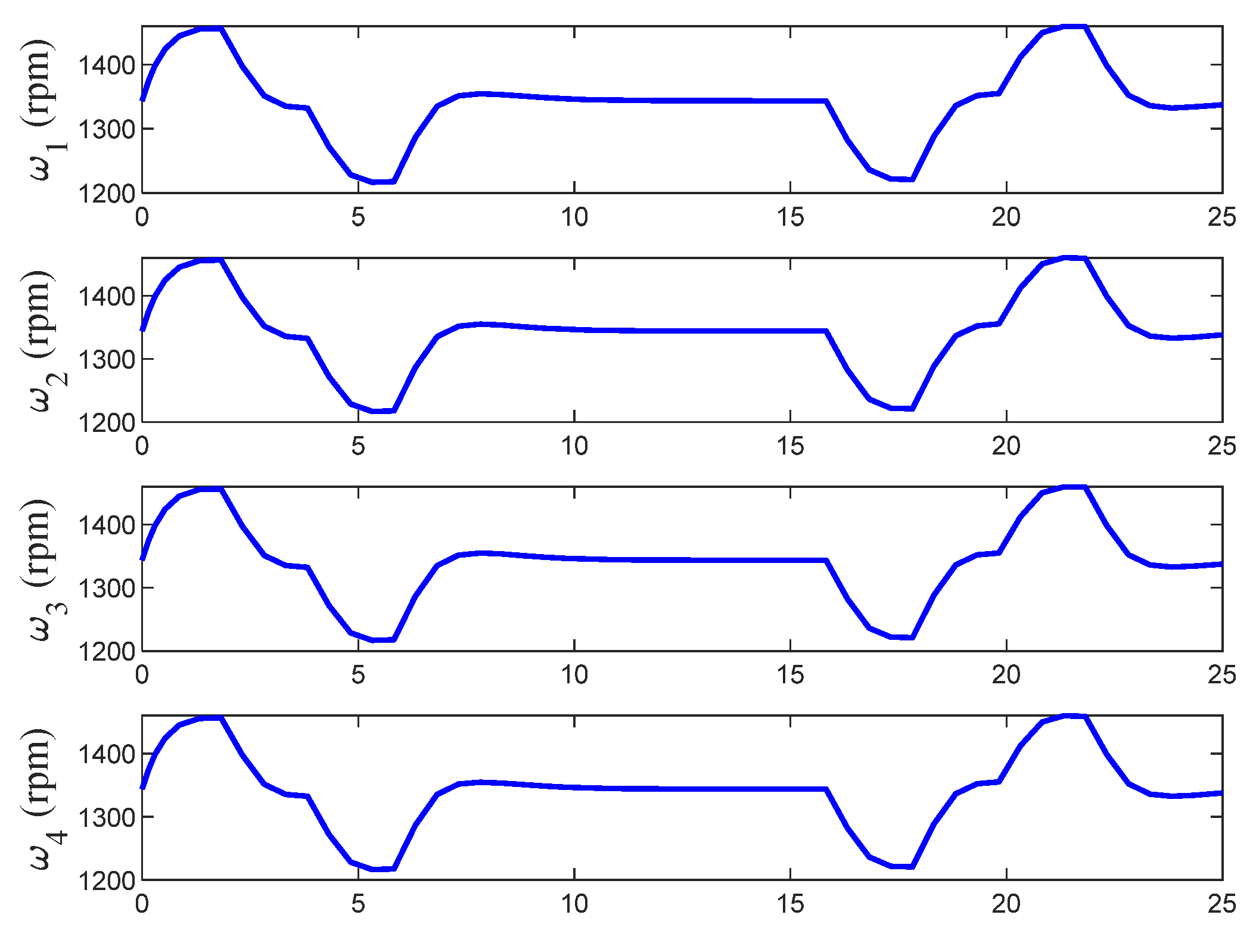
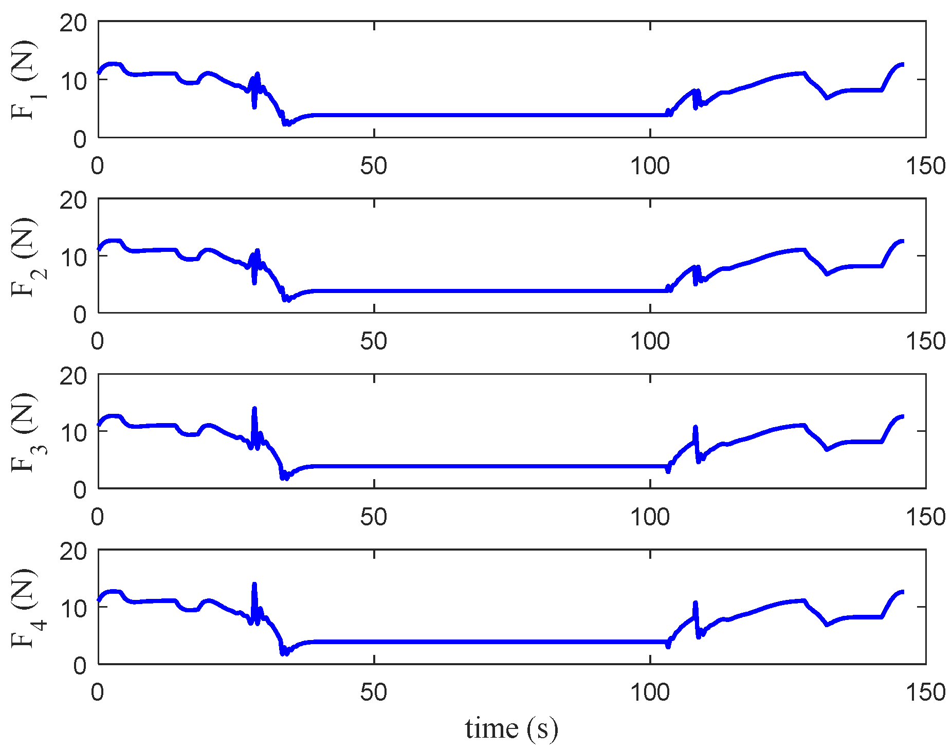
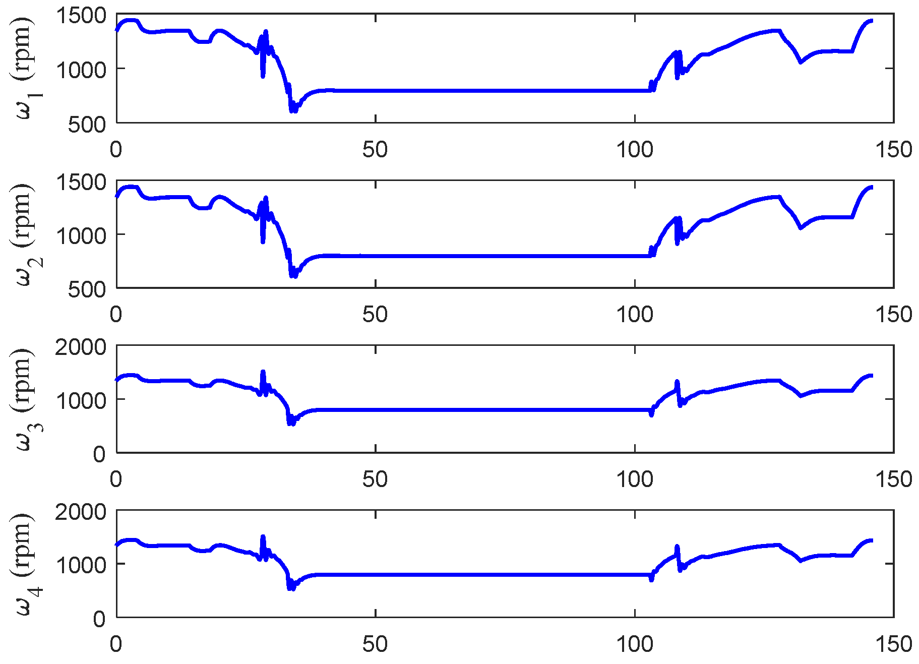
3.4. Motor RPM Calculations

Now, with the obtained control signals $U_1$ to $U_4$, the motor rotational speeds can be mapped to the control signals from the following expression:

$$\left[\begin{array}{c}{U}_1\\ U_2\\ U_3\\ U_4\end{array}\right]=\left[\begin{array}{cccc}\begin{array}{c}k\\ k{l}_s\\ k{l}_l\\ k\lambda \end{array}& \begin{array}{c}k\\ -k{l}_s\\ k{l}_l\\ -k\lambda \end{array}& \begin{array}{c}k\\ k{l}_s\\ -k{l}_l\\ -k\lambda \end{array}& \begin{array}{c}k\\ -k{l}_s\\ -k{l}_l\\ k\lambda \end{array}\end{array}\right]\left[\begin{array}{c}{\omega }_1^2\\ {\omega }_2^2\\ {\omega }_3^2\\ {\omega }_4^2\end{array}\right].$$

(64)

Conversely, in applying the inverse of this mapping, the motor speeds can be calculated directly from the control signals.

4. Simulation Results

This section presents the simulation results for controlling a quad-tilt-wing UAV using the nonlinear equations in Equation (19) and the parameters specified in

Table 1. QTW parameters.

Parameter	Value
$m$, QTW mass	4.5 kg
${\mathit{l}}_{\mathit{s}}$, spanwise distance between the rotors and the center of gravity (CG)	0.3 m
${\mathit{l}}_{\mathit{l}}$, longitudinal distance between the rotors and the center of gravity (CG)	0.3 m
$\mathit{\lambda }$, torque-to-thrust ratio	0.01

[11]. The simulations were performed in MATLAB/SIMULINK with a fixed time-step solver, set to 0.01 s. The variations in the lift coefficient, drag coefficient, and moment of inertia [34] are illustrated in Figure 5, Figure 6 and Figure 7. To evaluate the performance of the proposed controller, two scenarios were analyzed:

• Vertical Takeoff and Landing (VTOL): This scenario focuses on the QTW’s ability to execute precise vertical takeoff and landing maneuvers.
• Complete Longitudinal Motion: This scenario encompasses the entire flight sequence, including vertical takeoff, transition to cruise, cruising, transition back for landing, and vertical landing.

The control strategy was verified using Matlab/Simulink simulations, which provide a convenient platform for testing and analyzing the designed control laws before experimental implementation. However, we acknowledge that Matlab/Simulink does not inherently model all physical interactions, such as aerodynamic disturbances, ground contact dynamics, and other environmental effects that may influence real-world aircraft behavior. While the simulations accurately capture the system’s control dynamics and validate trajectory tracking performance, they do not fully replicate the complexities of a high-fidelity physics-based environment. To address this limitation, future work will include hardware implementation to further validate the proposed control algorithm under real-world conditions. This ensures that the developed control approach remains robust and applicable beyond simulation-based evaluations.

4.1. Scenario 1: Vertical Takeoff and Landing

In this scenario, the QTW performs a vertical ascent to an altitude of 12 m within 6 s, hovers steadily at this altitude for 10 s, and then descends and lands vertically over the course of 6 s. The 3D trajectory of this motion is illustrated in Figure 8, while the position and velocity profiles are shown in Figure 9 and Figure 10, respectively. Notably, a negative Z value indicates a position above the ground, as the Z-axis is defined pointing downward toward the ground.

Figure 11 demonstrates that the tilt angle was fixed at 90 degrees to provide sufficient thrust to counteract the mass of the QTW, with all Euler angles maintained at zero throughout the motion. The control signals are presented in Figure 12. Since the desired trajectory was purely vertical, only the ${\mathit{U}}_{\mathbf{1}}$ control signal was activated, while ${\mathit{U}}_{\mathbf{2}}$, ${\mathit{U}}_{\mathbf{3}}$, and ${\mathit{U}}_{\mathbf{4}}$ remained zero as there was no requirement for lateral motion or attitude adjustments.

Figure 13 depicts the ${\mathit{U}}_{\mathbf{1}}$ control signal in terms of the thrust generated by each motor, and Figure 14 illustrates the motor speeds.

4.2. Scenario 2: Complete Longitudinal Motion

This scenario involves a complete longitudinal motion sequence, including vertical takeoff, transition to cruise, cruising, transition back to landing, and vertical landing. The 3D trajectory of the QTW is shown in Figure 15. Figure 16 and Figure 17 compare the desired position and velocity with the actual results, demonstrating that the QTW closely followed the demanded trajectory. The QTW ascends over 18 s, reaching an altitude of 70 m to initiate the transition phase. The QTW then adjusts its tilt angle over 10 s to transition smoothly into cruise mode, achieving a speed of 12 m/s and maintaining it for 70 s. Following the cruise phase, the tilt angle is gradually increased over 20 s to prepare for a smooth transition back to vertical flight. Finally, the QTW descends and lands vertically within 18 s.

Figure 18 illustrates the tilt angle profile required for the mission. Initially, the tilt angle is set to 90 degrees for vertical takeoff. It then gradually decreases to 10 degrees within 10 s to facilitate a smooth transition and remains at this angle throughout the cruise phase. Finally, the tilt angle returns to 90 degrees during the transition back within 20 s and vertical landing. As shown in the figure, the pitch angle adjusts to enable the transition and cruise phases, while the roll and yaw angles remain at zero. During the transition phase, the pitch angle initially increases to approximately 50 degrees at the midpoint of the transition, before gradually decreasing. During the cruise phase, the pitch angle stabilizes at approximately 20 degrees, ensuring the necessary lift to sustain the cruise speed.

Figure 19 illustrates the angular velocity, highlighting that the pitch rate reaches a maximum of 0.5 rad/s at the midpoint of the transition. Figure 20 presents the control signals, where ${\mathit{U}}_{\mathbf{1}}$ is activated for altitude control and ${\mathit{U}}_{\mathbf{3}}$ for pitch control, while ${\mathit{U}}_{\mathbf{2}}$ and ${\mathit{U}}_{\mathbf{4}}$ remain zero, as roll and yaw adjustments are unnecessary.

Finally, the thrust and RPM of the motors are depicted in Figure 21 and Figure 22, providing further insights into the performance of the QTW during the mission.

5. Conclusions and Future Work

This paper demonstrated the effectiveness of an optimal control approach in managing the complex, nonlinear dynamics of quad-tilt-wing (QTW) systems. By employing State-Dependent Riccati Equation (SDRE) and Linear Quadratic Regulator (LQR) techniques for attitude and trajectory control, the proposed controller successfully managed the system in both vertical and longitudinal flight phases. The controller design, analytically solved for real-time implementation, ensures computational efficiency and practical feasibility.

The results highlight the efficacy and adaptability of the proposed control methodology, showing its capability to handle the unique challenges posed by the coupled dynamics of QTW systems. The successful control of vertical takeoff, cruise transitions, and longitudinal maneuvers demonstrates the potential for extending this framework to more complex flight scenarios.

Our future work will focus on enhancing the system’s autonomy and maneuverability. This includes the development of an automatic tilt angle adjustment mechanism and extending the control framework to enable precise 3D trajectory tracking. To achieve this, aerodynamic control surfaces will be integrated, and a strategy for distributing the required control moments between the motors and control surfaces will be implemented. Additionally, the developed control algorithms will be implemented on an experimental platform to assess their real-world efficacy and validate the proposed approach under practical conditions. These advancements aim to improve the vehicle’s agility, stability, and overall performance, paving the way for more versatile applications of QTW systems in real-world scenarios.