Multi-Altitude Corn Tassel Detection and Counting Based on UAV RGB Imagery and Deep Learning

Abstract

In the context of rapidly advancing agricultural technology, precise and efficient methods for crop detection and counting play a crucial role in enhancing productivity and efficiency in crop management. Monitoring corn tassels is key to assessing plant characteristics, tracking plant health, predicting yield, and addressing issues such as pests, diseases, and nutrient deficiencies promptly. This ultimately ensures robust and high-yielding corn growth. This study introduces a method for the recognition and counting of corn tassels, using RGB imagery captured by unmanned aerial vehicles (UAVs) and the YOLOv8 model. The model incorporates the Pconv local convolution module, enabling a lightweight design and rapid detection speed. The ACmix module is added to the backbone section to improve feature extraction capabilities for corn tassels. Moreover, the CTAM module is integrated into the neck section to enhance semantic information exchange between channels, allowing for precise and efficient positioning of corn tassels. To optimize the learning rate strategy, the sparrow search algorithm (SSA) is utilized. Significant improvements in recognition accuracy, detection efficiency, and robustness are observed across various UAV flight altitudes. Experimental results show that, compared to the original YOLOv8 model, the proposed model exhibits an increase in accuracy of 3.27 percentage points to 97.59% and an increase in recall of 2.85 percentage points to 94.40% at a height of 5 m. Furthermore, the model optimizes frames per second (FPS), parameters (params), and GFLOPs (giga floating point operations per second) by 7.12%, 11.5%, and 8.94%, respectively, achieving values of 40.62 FPS, 14.62 MB, and 11.21 GFLOPs. At heights of 10, 15, and 20 m, the model maintains stable accuracies of 90.36%, 88.34%, and 84.32%, respectively. This study offers technical support for the automated detection of corn tassels, advancing the intelligence and precision of agricultural production and significantly contributing to the development of modern agricultural technology.

1. Background

In modern agricultural production, the evaluation and monitoring of crop yields are essential for boosting agricultural productivity. Corn, being one of the most important food crops globally (Fischer et al., 2014) [1], has a direct impact on food security and economic development worldwide. Traditional methods of detecting tassels often involve manual visual inspection or basic mechanical devices, which are inefficient and influenced by environmental and weather conditions, leading to low detection accuracy. However, recent advancements in deep learning (Al-lQubaydhi et al., 2024) [2] and unmanned aerial vehicles have enabled researchers to develop automated toolsthat enhance the precision and efficiency of these tasks (Guan et al., 2024) [3], thereby making tassel detection more accurate and efficient.

The use of unmanned aerial vehicle imagery and deep learning for monitoring corn tassels allows the quantification of plant characteristics and assessment of plant health. This enables the development of more precise and effective management strategies. For example, farmers can predict yields based on the maturity of corn tassels, schedule harvest times appropriately, and avoid yield losses due to premature or delayed harvesting. Additionally, monitoring corn tassels facilitates the early detection and management of potential issues during growth stages, such as pests, diseases (Ntui et al., 2024) [4], and nutrient deficiencies, ensuring healthy growth and stable corn yields.

The monitoring of corn tassels also holds significant value for scientific research. By detecting and comparing corn tassels across different varieties and growth conditions (Yu et al., 2024) [5], researchers can gain insights into corn growth patterns and influencing factors. This knowledge provides strong support for genetic improvement and innovative cultivation techniques in corn production.

The automatic identification and counting of corn tassels using unmanned aerial vehicle imagery and deep learning allows agricultural professionals to estimate crop yields and assess crop health. These data support the advancement of modern agricultural technologies such as the agricultural Internet of Things and smart agriculture, fostering the intelligence and precision of agricultural production. Moreover, as a component of precision agriculture practices (Gong et al., 2024) [6], it helps farmers gain deeper understanding and control over their crops, ultimately leading to higher yields, lower costs, and minimized environmental impact.

The integration of deep learning models and unmanned aerial vehicles in agriculture holds significant potential for efficient large-scale crop monitoring. This research provides essential technical support for the development of precision agriculture and intelligent farming systems (John et al., 2024) [7], propelling agriculture towards modernization and sustainable development.

2. Introduction

2.1. Research Work by Relevant Scholars

Given the extensive research background on corn tassel identification and counting, this field has produced numerous notable scientific research results. This area of research has garnered significant attention from many researchers and has yielded a range of innovative and practical outcomes. These advancements not only drive the ongoing development of corn tassel detection technology, but also provide essential technical support for precision agriculture.

For instance, Kumar et al. [8] (2020) introduced a pixel-based segmentation method for detecting corn tassels and estimating growth stages, which markedly reduces the time required for creating CNN model training datasets and offers benefits in training time and computational complexity.

Liu et al. [9] (2020) enhanced Faster R-CNN for high-resolution corn tassel detection (5280 × 2970) by incorporating ResNet and VGGNet techniques, achieving satisfactory outcomes. However, they encountered the challenge of slow processing speeds.

Zan et al. [10] (2020) proposed an automatic detection algorithm for corn tassels using UAV imagery and deep learning techniques, combining random forest and VGG16. They successfully achieved accurate detection and branch extraction of tassels across different developmental stages, offering critical support for maize breeding and seed production. However, there were instances where leaf veins and reflective leaves were misidentified as tassels, resulting in certain errors. Additional validation and refinement are needed to enhance the practicality and stability of the algorithm.

Desai et al. [11] (2021) proposed a novel method for detecting maize crop tassels using k-means clustering and adaptive thresholding, demonstrating its performance closeness to reference methods through qualitative and quantitative analysis. Achieving precision of 0.97438, recall of 0.88132, and an F1 score of 0.92412, they also introduced a semi-automatic image annotation approach, enabling rapid generation of labeled datasets for maize crop with significant time savings in annotation.

Mirnezami et al. [12] (2021) introduced an automated process that combines deep learning and image processing techniques to extract maize tasseling and flowering patterns from time-lapse camera images under field conditions. They demonstrated the method’s effectiveness in tassel detection, classification, and segmentation, providing a robust tool for studying maize reproductive development. Nonetheless, this method encounters difficulties with multiple and sub-target detections.

Ji et al. [13] (2021) proposed a novel automated approach for maize tassel detection, incorporating a color attenuation prior model and the Itti visual attention detection algorithm, along with texture features and vegetation indices. They successfully achieved accurate detection of maize tassels in stable field images, with a recall rate, precision, and F1 score of 86.30%, 91.44%, and 88.36%, respectively, though the accuracy was moderate.

Alzadjali et al. [14] (2021) evaluated two automatic maize tassel detection methods: one based on the temporal-difference convolutional neural network (TD-CNN) and the other on Faster R-CNN. Both methods achieved satisfactory results, with F1 scores of 95.9% and 97.9%, respectively. Nonetheless, these methods face challenges such as long model training times, complex network structures, slow detection speeds, high costs, and suboptimal performance in detecting small targets.

Liu et al. [15] (2022) proposed a novel algorithm named YOLOv5-tassel, which achieved precise detection of maize tassels in RGB images captured by unmanned aerial vehicles. The algorithm innovatively introduced a bidirectional feature pyramid network, SimAM attention module, and transfer learning, resulting in an mAP value of 44.7% under limited data, surpassing traditional object detection methods, such as FCOS, RetinaNet, and YOLOv5. However, this version of the method lags behind in accuracy, speed, and computational efficiency compared to the latest deep learning models.

Pu et al. [16] (2023) proposed a model named Tassel-YOLO, which utilizes UAV imagery for automatic detection and counting of maize tassels, significantly enhancing detection accuracy and real-time performance. This model incorporates a global attention mechanism, specific convolutional structures, and loss function optimization, leading to a reduction in parameters and computational costs, while achieving a detection accuracy of 97.55%. However, this approach suffers from poor dataset quality and detects tassels at heights too close to the ground.

Zhang et al. [17] (2023) introduced a new maize tassel detection model named SwinT-YOLO. They optimized the backbone of YOLOv4 using the Swin transformer and implemented depthwise separable convolution modules to decrease the model’s parameters and FLOPs. This resulted in a maize tassel recognition accuracy of 95.11%. However, the method faced challenges such as poor image quality, high computational demands on UAVs, and limited detection robustness.

Ye et al. [18] (2023) introduced WheatLFANet, a high real-time, lightweight neural network for wheat spike detection. The model achieved an average precision (AP) of 90% and an R² value of 0.949 between predicted values and ground truth. It operates an order of magnitude faster than other state-of-the-art methods, suggesting the feasibility of achieving real-time, lightweight wheat spike detection on low-end devices with strong generalization ability. However, the model’s robustness is limited, making it challenging to apply in complex scenarios.

Jia et al. [19] (2024) proposed an effective method for maize tassel detection by incorporating a channel attention (CA) mechanism into the backbone of YOLOv5, achieving an average precision of 96%. This approach effectively detects early-stage maize tassels and manages challenges such as leaf occlusion and complex backgrounds. However, the method requires high-quality images and has limitations due to its proximity to the ground.

Rodene et al. [20] (2024) utilized a UAV aerial image dataset to develop a machine learning method based on object detection and regression, enabling automated maize tassel counting at the plot level. Through image segmentation and filtering techniques, significant improvements in counting accuracy were achieved, providing reliable tools and decision support for crop improvement.

Wu et al. [21] (2024) collected corn tassel images under various environmental conditions using UAVs and developed an ESG-YOLO detection model based on the YOLOv7 model. The ESG-YOLO model achieved an average accuracy of 93.1%, which is 2.3 percentage points higher than the original YOLOv7 model, providing an efficient approach for the automatic identification of corn tassel density. Nonetheless, this method may not be suitable for large-scale, multi-target detection tasks.

Despite these advancements, a critical issue remains unaddressed; the recognition and counting of corn tassels at different heights, not just close to the ground. The impact of deep learning models on corn tassel recognition and counting performance at varying heights warrants further investigation.

2.2. Contribution of This Article

Building upon the excellent research achievements of the aforementioned scholars, and considering the practical agricultural production environment, we propose a method utilizing YOLOv8 and unmanned aerial vehicles for maize tassel recognition and counting at different heights (5 m, 10 m, 15 m, 20 m), as depicted in Figure 1. The main contributions of this paper are as follows:

(1)

We present a high-quality dataset of corn tassels captured by unmanned aerial vehicles (UAVs), consisting of images with a resolution of 5280 × 2970 pixels and an aspect ratio of 4:3. The dataset includes images taken at heights of 5 m, 10 m, 15 m, 20 m, 30 m, and 50 m, with 500 images per height;

(2)

In order to reduce the parameter count and computational complexity in multi-target corn tassel recognition tasks, achieve lightweight network models, and improve target detection speed, we introduced Pconv convolution in the backbone section of YOLOv8. Additionally, we incorporated the ACmix module to enhance feature extraction by capturing local features through convolution, which was particularly beneficial for single-class corn tassel detection tasks;

(3)

We introduced the CTAM module in the neck section to enhance feature fusion and improve semantic information correlation between channels. This measure facilitates accurate and efficient localization of corn tassels and precise identification of their boundary features;

(4)

We proposed a learning rate optimization method based on the sparrow search algorithm (SSA) to obtain the optimal learning rate for the highest average precision, thereby enhancing the model’s robustness and detection accuracy;

(5)

With the improved YOLOv8 model, we achieved an accuracy of 97.59%, a recall rate of 94.40%, a frame rate of 40.62 FPS, model parameters of 14.62 MB, and GFLOPs of 11.21. These results demonstrate the model’s capability to undertake large-scale corn tassel recognition and counting tasks with UAVs under complex conditions [22].

3. Experimental Materials and Data

3.1. Acquisition of Corn Tassel Images

Corn tassel sample images were collected in the Hexi Corridor of Gansu Province, China (100°49′ E, 38°25′ N), which is known as the largest maize seed production base in the country. This region experiences a temperate continental climate characterized by dryness, low precipitation, frequent sandstorms, and long sunshine hours. To capture the images, we utilized the DJI Mavic 3 Class unmanned aerial vehicle (UAV), featuring a maximum flight time of 46 min and resistance to wind speeds of up to 12 m/s, making it suitable for the region’s challenging climatic conditions. Equipped with a 20-megapixel Hasselblad imaging system, the UAV captures images at a resolution of 5280 × 2970 pixels, with an aspect ratio of 4:3 and a file size of approximately 13.2 MB, enabling the collection of highly detailed photographs that meet the requirements for corn tassel image acquisition. A total of 3000 images were gathered at heights of 5 m, 10 m, 15 m, 20 m, 30 m, and 50 m, as depicted in Figure 2.

3.2. Dataset Creation

The 3000 corn tassel images, collected at different heights, underwent annotation using LabelImg (version 1.8.6) data annotation software. This process resulted in annotation information containing the coordinates of the corn tassel center points, as well as the width and height of the bounding boxes, which were saved in txt format. Subsequently, the dataset was divided into training, validation, and test sets in an 8:1:1 ratio [17].

Moreover, various data augmentation techniques were applied, including Mosaic, Affine, Perspective, Copy-Paste, HSV, and Mixup. These techniques were instrumental in enhancing the model’s generalization ability and robustness, while mitigating the risk of overfitting.

3.3. Experimental Environment and Parameter Settings

All computational resources utilized in this experiment were provided by the A800 deep learning server housed in the Intelligent Sensing and Control Laboratory at Shandong University of Petroleum and Chemical Engineering. The specific model of the server is NF5468M6. The software configuration of the server includes the CentOS Linux 7 operating system, 125.4 GiB of RAM, a 1.9 TB hard disk, and GNOME version 3.28.2. In terms of hardware configuration, the server features an Intel Xeon(R) Silver 4314 CPU with a clock speed of 2.4 GHz and 64-bit architecture, llvmpipe (LLVM 7.0, 256 bits) as the image renderer, and an NVIDIA A800 80 GB PCIe × 2 graphics card. The deep learning environment is configured with Python version 3.8.13, CUDA version 11.3, and PyTorch version 1.7.1.

4. The YOLOv8 Network Model

4.1. The Structure of YOLOv8

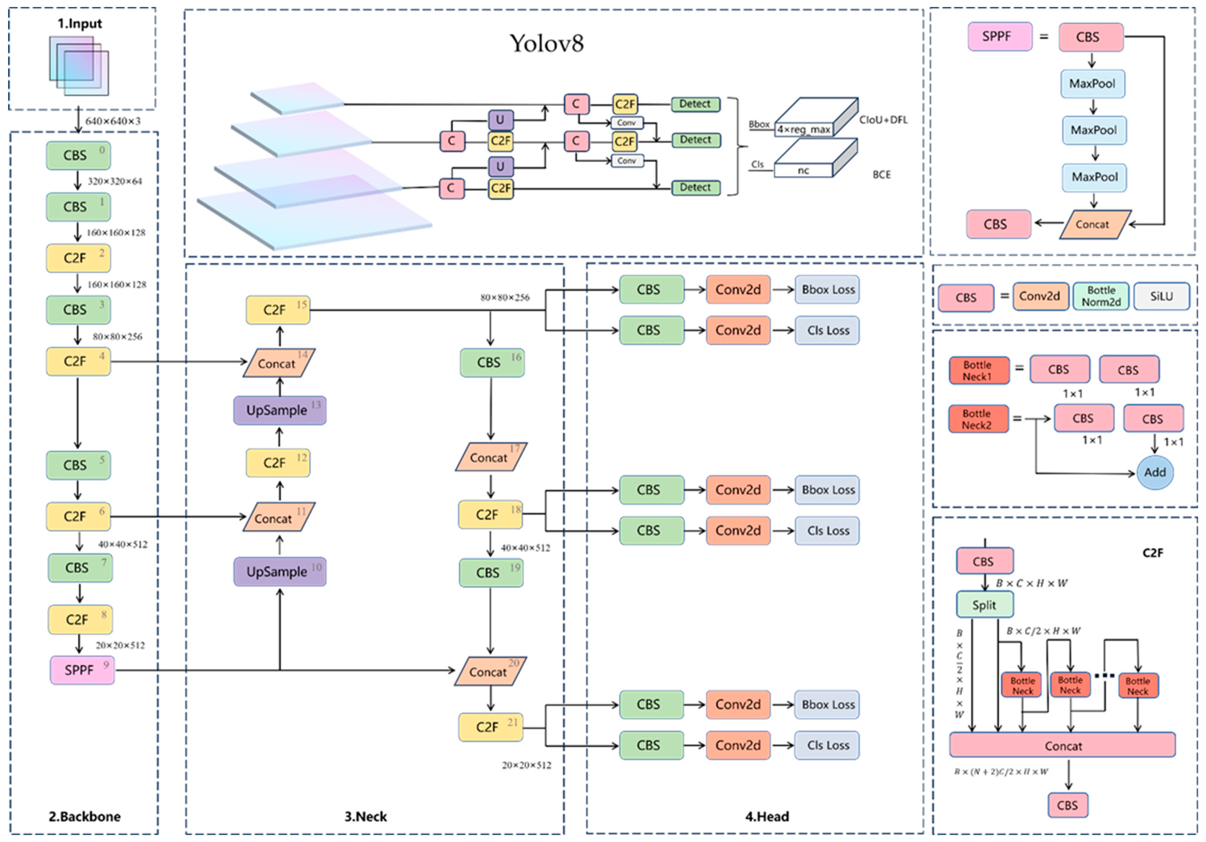
Yolov8 [23] stands as one of the prominent representatives within the YOLO series algorithms for object detection. It excels in tasks such as detection, classification, and instance segmentation. Its specific network structure is depicted in Figure 3. Released in January 2023, Yolov8 has garnered widespread attention and adoption in the industrial domain, owing to its efficiency, accuracy, and adaptability. Yolov8 offers target detection networks with resolutions including P5 (640) and P6 (1280), as well as an instance segmentation model based on YOLACT. Similarly to Yolov5, Yolov8 provides models of different sizes, such as N/S/M/L/X scales, to accommodate various tasks and scenarios. For this study, we utilize the S version, which is well-suited for object detection tasks on certain mobile devices or embedded systems.

The backbone section comprises three modules: CBS, C2F, and SPPF. The CBS module integrates convolution (Conv), batch normalization (BN), and Sigmoid Linear Unit (SiLU) activation function components [24]. For the neck section, the PAnet structure is adopted to facilitate feature fusion across multiple scales. Both the backbone and neck sections are influenced by the ELAN design concept from Yolov7. The C3 module in Yolov5 is replaced by the C2F module, enhancing gradient information richness. Channel numbers are adjusted for models of different scales, no longer applying a uniform set of parameters to all models, thereby significantly enhancing model performance. However, operations like Split in the C2F module may increase computational complexity and parameterization excessively.

Compared to Yolov5, Yolov8’s head section incorporates two significant enhancements. Firstly, it adopts the widely utilized decoupled-head structure, which separates the classification and detection heads. Secondly, it implements an anchor-free design, eliminating the need for anchors.

In the loss section, Yolov8 departs from previous practices of IOU matching or single-side proportion allocation, opting instead for the task-aligned assigner for positive and negative sample matching [25]. Additionally, it introduces the distribution focal loss (DFL).

In the training section, Yolov8 integrates the data augmentation strategy from YoloX, which involves disabling the Mosaic augmentation operation in the final ten epochs. This adjustment effectively enhances the model’s accuracy.

4.2. PConv Module

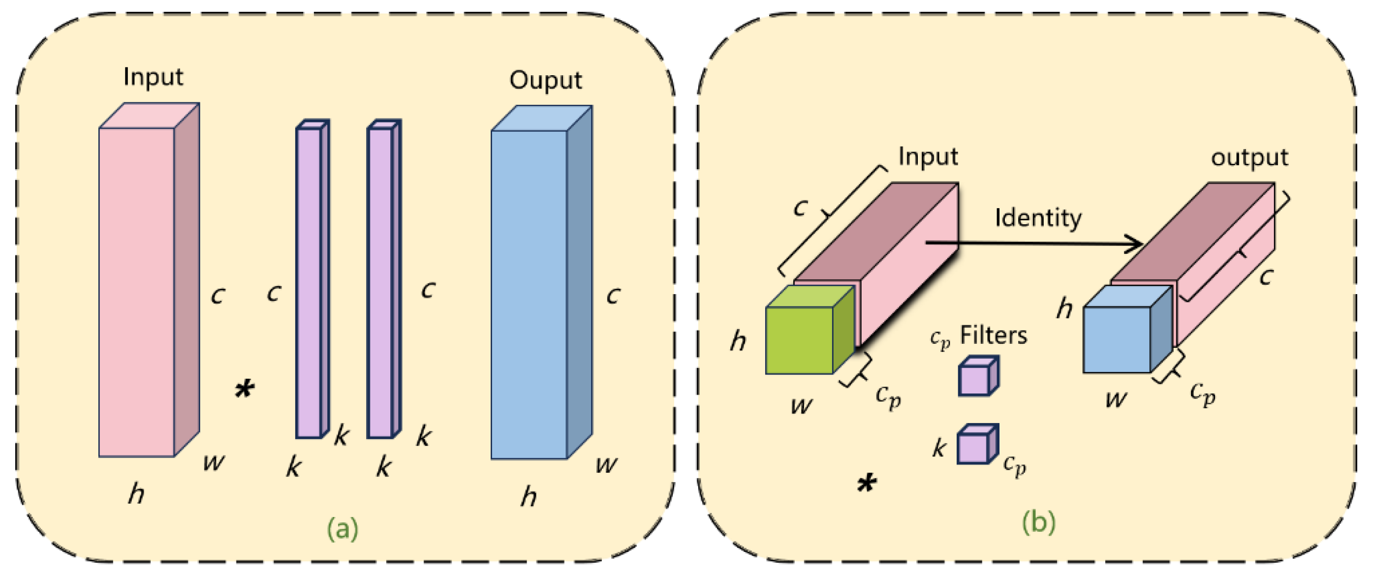
To achieve a lightweight model and enhance detection speed, numerous improvements have concentrated on reducing the number of floating-point operations (FLOPs). However, simply reducing FLOPs may not necessarily result in equivalent speed enhancements [26]. This is because the frequent memory access associated with conventional convolutions can lead to inefficient floating-point operations. To address this issue, a novel convolution method called partial convolution (PConv) is introduced in the backbone section. PConv effectively reduces redundant computations and memory accesses by applying filters to only select input channels, while leaving others untouched. The conventional convolution structure is depicted in Figure 4a, while the PConv convolution is illustrated in Figure 4b.

PConv leverages redundancy within feature maps by selectively applying conventional convolution to a portion of input channels, while leaving the remainder unchanged [27]. Given that this paper’s object detection task focuses solely on the maize tassel category, deep convolution operations for feature extraction are unnecessary. Thus, we substitute Conv2d in the multi-branch stacking module of the C2F module with PConv, as illustrated in Figure 5.

The computational cost of PConv is expressed by Equation (1), where the convolution ratio of typical features is denoted by r. The memory computational cost of PConv is represented by Equation (3).

$$h\times w\times k^2\times c_p^2$$

(1)

$$r=\frac{c_p}{c}=\frac{1}{4}$$

(2)

$$h\times w\times 2c_p+k^2\times c_p^2\approx h\times w\times 2c_p$$

(3)

In the aforementioned equations, h represents the height of the feature channel, w represents the width of the feature channel, cp represents the continuous network channels, and k represents the filter [28].

In tackling the challenge of limited computing power in drone systems for multi-target maize tassel detection tasks, there arises a concern regarding the large network model size and computational demands, leading to sluggish inference speeds. Hence, this paper introduces PConv convolution in the backbone section to alleviate the parameter count and computational load in target detection tasks. This approach aims to achieve a lightweight network model and enhance target detection speed.

4.3. Introducing the ACmix Module in the Backbone Network to Enhance Feature Extraction

When utilizing drones at heights of 10 m or 15 m, as well as at greater heights, the demand for extracting detailed features becomes more critical. Moreover, small object detection boxes are susceptible to blending with larger proportions of complex backgrounds. In this study, we employed the ACmix module to prioritize the extraction of key targets in the feature maps, specifically focusing on corn tassels. The ACmix module is a hybrid model that amalgamates the strengths of self-attention mechanisms and convolutional operations. This integration allows the leveraging of the global perceptual abilities of self-attention, while capturing local features through convolution, which proves highly advantageous for tasks involving only one class of target, such as corn tassel detection. By adopting this approach, we maintain relatively low computational costs while enhancing the model’s performance. The structure of the ACmix mechanism is depicted in Figure 6, where C, H, and W represent the number of channels, width, and height of the feature map, respectively [29]. K denotes the kernel size, and a and b are learning factors for convolution and self-attention, respectively. The ACmix mechanism comprises two stages.

In the initial stage, known as the feature projection stage, the input features undergo three 1 × 1 convolutions, thereby reshaping them into N feature segments. This process yields a comprehensive feature set comprising 3N feature maps, thus furnishing robust support for subsequent feature fusion and aggregation [30].

The second stage is the feature aggregation and fusion stage, where information is collected through different paths. For convolutional paths with a kernel size of k, a lightweight fully connected layer is first used to generate k² feature maps. These feature maps are then assembled into N groups, each containing three features, corresponding to query, key, and value. Let $f_{ij}$ and $g_{ij}$ represent the input and output tensors, and $X_u\left(i,j\right)$ denote the local pixel region centered at (i, j), with a spatial width of u. Then $A\left(W_q^{\left(l\right)}{f}_{ij},W_k^{\left(l\right)}{f}_{ab}\right)$ represents the weights corresponding to $X_u\left(i,j\right)$, where a, b ∈ $X_u\left(i,j\right)$. The convolutional path operation is detailed in Equation (4). Following this operation, the feature maps undergo shifting and aggregation processes, enabling the gathering of information from local receptive fields. The resulting output from the convolutional path encapsulates the local details and texture information of the input features.

$$A\left(W_q^{\left(l\right)}{f}_{ij},W_k^{\left(l\right)}{f}_{ab}\right)=\genfrac{}{}{0pt}{}{softmax}{X_u\left(i,j\right)}\left(\frac{{\left(W_q^{\left(l\right)}{f}_{ij}\right)}^T{\left(W_k^{\left(l\right)}{f}_{ab}\right)}^T}{\sqrt{d}}\right)$$

(4)

In this equation, $W_q^{\left(l\right)}$ and $W_k^{\left(l\right)}$ are projection matrices for query and key, respectively. d represents the feature dimension of $W_q^{\left(l\right)}{f}_{ij}$, and softmax denotes the softmax normalization function. The multi-head self-attention mechanism is decomposed into two stages, as shown in Equations (5) and (6).

$$\left\{\begin{array}{c}{q}_{ij}^{\left(l\right)}=W_q^{\left(l\right)}{f}_{ij}\\ k_{ij}^{\left(l\right)}=W_k^{\left(l\right)}{f}_{ij}\\ v_{ij}^{\left(l\right)}=W_v^{\left(l\right)}{f}_{ij}\end{array}\right.$$

(5)

$$g_{ij}=\begin{array}{c}N\\ \parallel \\ l=1\end{array}(\sum _{a,b\in X_u(i,j)}A(q_{i,j}^{\left(l\right)},k_{ab}^{\left(l\right)})v_{ab}^l)$$

(6)

In the above equations, $W_q^{\left(l\right)}$, $W_k^{\left(l\right)}$, and $W_v^{\left(l\right)}$ are projection matrices for query, key, and value at pixel (i, j), respectively. $q_{ij}^{\left(l\right)}$, $k_{ij}^{\left(l\right)}$, and $v_{ij}^{\left(l\right)}$ are feature map matrices after the projection of query, key, and value. $\parallel$ denotes the concatenation of outputs from N attention heads. Through computing the similarity between queries and keys, attention weights are derived. These weights are subsequently employed to aggregate values in a weighted manner, thereby generating the output of the self-attention pathway.

Finally, the ultimate output $F_{out}$ of ACmix is obtained by adding the outputs from both the convolutional pathway and the self-attention pathway, as shown in Equation (7). Here, the parameters $\alpha$ and $\beta$ can be adjusted based on the relative importance of global and local weights.

$$F_{out}=\alpha F_{att}+\beta F_{conv}$$

(7)

4.4. Introducing the CTAM Module into the Neck Network to Enhance Feature Fusion

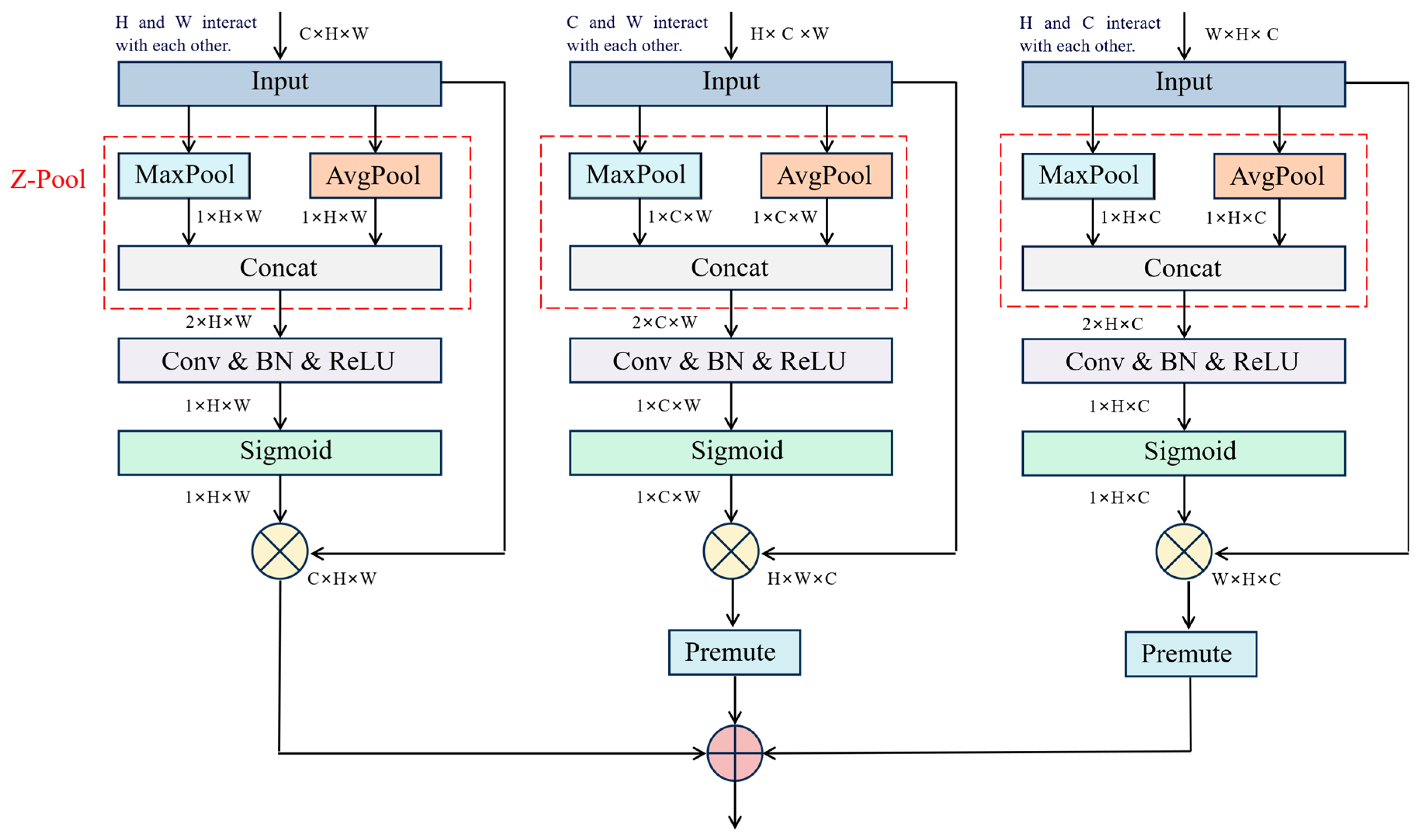
In contrast to the methods of CBMA [31] and SENet [32], which learn channel dependencies through two fully connected layers involving dimension reduction followed by dimension increase, the CTAM module proposed in this paper employs an almost parameter-free attention mechanism to model channel and spatial attention. This approach establishes a cost-effective and efficient channel attention mechanism. The attention mechanism effectively captures connections between different modal features, diminishes the interference of unimportant information, and enhances the semantic information correlation between channels. Consequently, this facilitates accurate and efficient localization of maize tassels and identification of their boundary features. The structure of CTAM is depicted in Figure 7.

The input tensor ${X\in R}^{(C\times H\times W)}$ enters the first branch to establish interaction between the H and W dimensions. After Z-pooling, a simplified tensor x of shape (2 × H × W) is obtained. Subsequently, through Conv, BN, and ReLU operations, attention weights of shape (1 × H × W) with batch normalization are obtained. Then, the tensor x₁ is passed through a sigmoid activation layer to generate attention weights. Finally, the attention weights are applied to the input tensor X, resulting in the output tensor $\widehat{x_1}$.

The input tensor ${X\in R}^{(C\times H\times W)}$ enters the second branch to establish interaction between the C and W dimensions. Through a transpose operation, a rotated tensor $\widehat{x_2}$ of shape (H × C × W) is obtained. Subsequently, after Z-pooling, a tensor $\widehat{x_2^{\ast }}$ of shape (2 × C × W) is obtained. Then, through Conv, BN, and ReLU operations, a middle output tensor of shape (1 × C × W) with batch normalization is obtained. Afterwards, the tensor is passed through a sigmoid activation layer to generate attention weights. Finally, a transpose operation is performed to obtain a tensor with the same shape as the input.

Then, the tensor ${X\in R}^{(C\times H\times W)}$ is passed through the third branch to establish interaction between the H and C dimensions. Through a transpose operation, a rotated tensor $\widehat{x_3}$ with a shape of (W × H × C) is obtained. Subsequently, after passing through Z-pool, a tensor $\widehat{x_3^{\ast }}$ with a shape of (2 × H × C) is obtained. Then, through Conv, BN, and ReLU, a batch-normalized tensor with a shape of (1 × H × C) is generated as intermediate output. Next, the tensor is passed through a sigmoid activation layer to generate attention weights. Finally, a transpose operation is applied to obtain a tensor with the same shape as the input [33].

Finally, the outputs of the three branches are aggregated to generate a fine tensor (C × H × W). The formula for computing the output tensor is as follows:

$$y=\frac{1}{3}\left(x_1\sigma \left({\phi }_1\left(\widehat{x_1}\right)\right)+\overline{\widehat{x_2}\sigma \left({\phi }_2\left(\widehat{x_2^{\ast }}\right)\right)}+\overline{\widehat{x_3}\sigma \left({\phi }_3\left(\widehat{x_3^{\ast }}\right)\right)}\right)$$

(8)

4.5. Learning Rate Optimization Based on Sparrow Search Algorithm

In the YOLO series of models, learning rate optimization plays a crucial role, directly influencing both the training speed and the final recognition accuracy of the model. Setting the learning rate too high can lead to divergence during training, preventing the model from converging to the optimal solution. Conversely, setting the learning rate too low may result in slow training speeds and could potentially cause the model to become trapped in local optima. Inspired by intelligent heuristic algorithms and evolutionary algorithms, we propose a learning rate optimization method based on the sparrow search algorithm (SSA). This method aims to determine the optimal learning rate corresponding to the highest average precision, thereby enhancing the robustness and detection accuracy of the model.

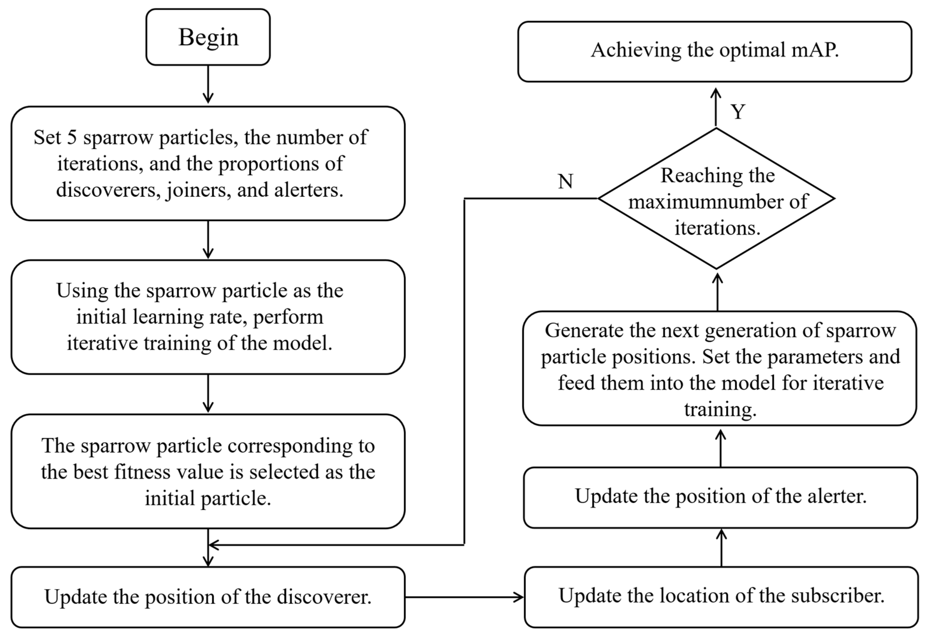
The sparrow search algorithm (SSA) emulates the foraging, clustering, jumping, and evasion behaviors observed in sparrows as they navigate solution spaces, continuously updating their positions [34]. Acting as leaders, sparrows guide the search for food, while followers trail behind to forage and compete with each other to enhance predation rates. Vigilant sparrows abandon foraging upon detecting danger. Each sparrow represents a solution, tasked solely with locating the food source. The flowchart outlining the SSA is presented in Figure 8.

(1) Set the parameters for the sparrow search algorithm (SSA), including the number of sparrow particles, the number of iterations, and the ratio of explorers, joiners, and vigilants. Let us assume there are N sparrow individuals in a D-dimensional search space, with the initial population represented as $x_i$ = [$x_{i1},x_{i2},\dots \dots ,x_{iD}$], where i = 1, 2, …, N and d = 1, 2, …, D. Here, $x_{id}$ represents the position of the ith sparrow in the D-dimensional search space. The fitness function is denoted as $f_i=f(x_1,x_2,\dots \dots ,x_{\mathrm{D}})$. The ratio of discoverers to joiners is determined by Equations (10) and (11).

$$r=b\left(\mathrm{t}\mathrm{a}\mathrm{n}\left(-\frac{\pi t}{{4iter}_{\mathrm{m}\mathrm{a}\mathrm{x}}}+\frac{\pi }{4}\right)-k.\mathrm{r}\mathrm{a}\mathrm{n}\mathrm{d}(\mathrm{0,1})\right)$$

(9)

$$\mathrm{p}\mathrm{N}\mathrm{u}\mathrm{m}=rN$$

(10)

$$\mathrm{s}\mathrm{N}\mathrm{u}\mathrm{m}=(1-r)N$$

(11)

In the above equations, $\mathrm{p}\mathrm{N}\mathrm{u}\mathrm{m}$ represents the number of discoverers, $\mathrm{s}\mathrm{N}\mathrm{u}\mathrm{m}$ represents the number of joiners. $b$ is the scaling factor used to control the number of discoverers and joiners. $k$ is the perturbation factor used to perturb the non-linearly decreasing value $r$. ${iter}_{\mathrm{m}\mathrm{a}\mathrm{x}}$ represents the maximum number of iterations.

(2) Utilizing the initial learning rate obtained from the sparrow example, the validation set’s mean average precision (mAP) is employed as the fitness function for model iteration training. The objective of this process is to identify the sparrow position associated with the optimal fitness value;

(3) Updating the position of discoverers involves the following calculation formula:

$$x_{id}^{t+1}\left\{\begin{array}{c}{x}_{id}^t·\exp \left(\frac{-i}{\alpha ·t_{\mathrm{m}\mathrm{a}\mathrm{x}}}\right),(R_2<S_T)\\ x_{id}^t+P·L,(R_2\ge S_T)\end{array}\right.$$

(12)

In Formula (12), $x_{id}$ represents the position of the i-th sparrow at the t-th iteration. $\alpha$ and $P$ are uniformly distributed random numbers, where $\alpha$ and $P$ in (0, 1]. $t_{\mathrm{m}\mathrm{a}\mathrm{x}}$ is the maximum number of iterations. $R_2$ represents the alert value, where $R_2$ in [0, 1]. $S_T$ belongs to the safety value, where $S_T$ in [0.5, 1]. L is a matrix with elements equal to 1;

(4) When updating the position of joiners, the calculation formula is as follows:

$$x_{id}^{t+1}\left\{\begin{array}{c}P·\exp \left(\frac{x_{wd}^t-x_{id}^t}{i^2}\right),\left(i>\frac{N}{2}\right)\\ x_{id}^{t+1}+\left|x_{id}^t-x_{bd}^{t+1}\right|A^{+}·L,(i\le \frac{N}{2})\end{array}\right.$$

(13)

In Equation (13), $x_{wd}^t$ represents the worst position of the sparrows in the t-th iteration. $x_{id}^{t+1}$ represents the best position of the sparrows in the (t + 1)-th iteration. A represents a 1 × d matrix where elements are arbitrarily assigned as 1 or −1;

(5) The position update formula for the “watcher” is set as:

$$x_{id}^{t+1}\left\{\begin{array}{c}{x}_{bd}^t+\beta (x_{id}^t-x_{bd}^t),(f_i\ne f_g)\\ x_{id}^t+K\left(\frac{x_{id}^t-x_{wd}^t}{\left|f_i-f_w\right|+\tau }\right),(f_i=f_g)\end{array}\right.$$

(14)

In Equation (14), $x_{bd}^t$ represents the best position of the sparrow in the t-th iteration. B is the step size parameter. $f_i$ denotes the fitness value of the i-th sparrow. $f_g$ represents the current global best fitness value. $f_w$ represents the current global worst fitness value [35]. K is a random value for sparrow movement direction, where k∈[−1, 1]. $\tau$ is an infinitesimal constant;

(6) Generate the parameters for the next generation of sparrow particles and se-quentially feed them into the model for iterative training;

(7) Determine whether the maximum number of iterations has been reached. If so, end the program and output the results. Otherwise, repeat steps (3) to (6).

Using the learning rate optimization based on the sparrow search algorithm can accelerate the convergence speed of the model, improve its performance, mitigate overfitting during training, and enhance the model’s robustness. This effectively alleviates issues such as the increase in surface temperature of the drone due to intense sunlight, which could lead to overheating of electronic components and reduced battery life.

4.6. The Improved YOLOv8 Architecture Diagram

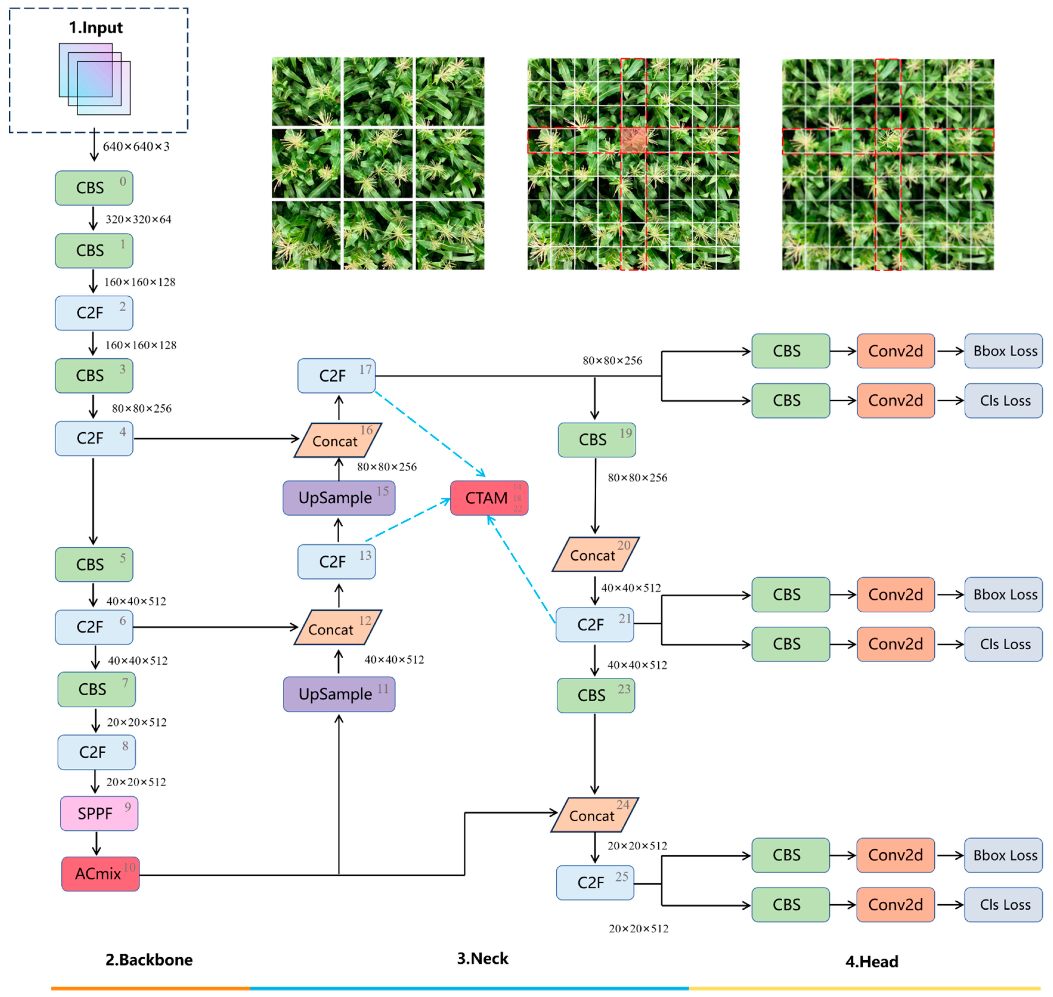
This paper primarily focuses on four key improvements to Yolov8. Firstly, the introduction of the Pconv local convolution module facilitates lightweight design and enables rapid detection speed. Secondly, the incorporation of the ACmix module in the backbone section combines the global perceptual ability of self-attention with convolution’s capability to capture local features, thereby enhancing feature extraction. Thirdly, the implementation of the CTAM module in the neck section enhances semantic information exchange between channels, ensuring accurate and efficient positioning of maize tassels and augmenting feature fusion capability. Lastly, by employing the sparrow search algorithm (SSA) to optimize the mean average precision (mAP), the model’s robustness and detection accuracy are enhanced. This optimization strategy effectively addresses the potential issues encountered by drones in intense lighting conditions, such as increased surface temperature and shortened battery life. The specific Yolov8 structure, following these improvements, is illustrated in Figure 9.

5. Experimental Results and Analysis

5.1. Learning Rate Optimization Based on Sparrow Search Algorithm

When detecting maize tassels, false positives and false negatives are common issues. Hence, to assess the precision of a model’s detection performance, accuracy metrics such as precision (P, %), recall (R, %), parameter count, frames per second (FPS), and floating point operations per second (GFLOPs) are commonly employed. Precision (P) denotes the ratio of correctly predicted samples among all samples predicted as positive, as illustrated in Formula (15).

$$P=\frac{T_P}{T_P+F_P}\times 100\%$$

(15)

Recall (R) represents the proportion of correctly predicted samples among all actual positive samples, as shown in Formula (16).

$$R=\frac{T_P}{T_P+F_N}\times 100\%$$

(16)

In the above formulas, $T_P$ represents the number of samples predicted as positive with positive labels, $F_P$ represents the number of samples predicted as positive with negative labels, and $F_N$ represents the number of samples predicted as negative with positive labels. Mean average precision (mAP) is a commonly used performance evaluation metric in object detection tasks, especially in multi-class object detection [36]. A higher mAP value indicates better detection performance, as shown in Formula (17).

$$mAP=\frac{\sum AveragePrecision\left(c\right)}{Num\left(cls\right)}$$

(17)

In this formula, AveragePrecision(c) represents the average precision of a certain class and Num(cls) is the number of all classes in the dataset. In this paper, the object detection task only involves one class, which is maize tassels. Therefore, mAP is equal to AP, which is precision.

FPS (frames per second) measures the number of frames processed per second and serves as a critical indicator for assessing the speed of computer graphics processing. Within the domains of computer vision and image processing, FPS denotes the rate at which a computer or algorithm processes a sequence of images, quantifying the number of frames processed within one second.

Params are utilized to evaluate the size and complexity of a model, derived by summing the number of weight parameters in each layer.

GFLOPs (giga floating point operations per second) represent the quantity of floating-point operations executed by the model per second during inference. This metric is employed to assess the computational complexity and performance of the model.

5.2. The Improved Model Compared to the Original Model

Figure 10 illustrates the comparison between the proposed model and the original Yolov8 concerning precision throughout the training process [37]. The analysis reveals that the proposed model surpasses the original Yolov8 in all aspects, notably in precision, demonstrating a marked enhancement.

During the initial 0 to 100 epochs, the precision of the improved model exhibits a rapid ascent from a relatively low level, indicating its adeptness at swiftly assimilating information in the early learning phase. Conversely, Yolov8 demonstrates a slower initial precision increase, followed by a gradual acceleration, albeit with a constrained growth rate.

Between 100 and 200 epochs, the precision growth of the improved model begins to decelerate, eventually stabilizing with minor fluctuations, suggesting that the model may have attained a relatively optimal state. Meanwhile, Yolov8 continues to experience a gradual precision increase, albeit at a limited overall growth rate.

From 200 to 500 epochs, the precision of the improved model exhibits slight fluctuations but maintains a relatively high level (97.59), indicating its sustained generalization capability, albeit potentially facing overfitting risks. In contrast, the precision of Yolov8 stabilizes around 94.32 and fluctuates within a narrow range.

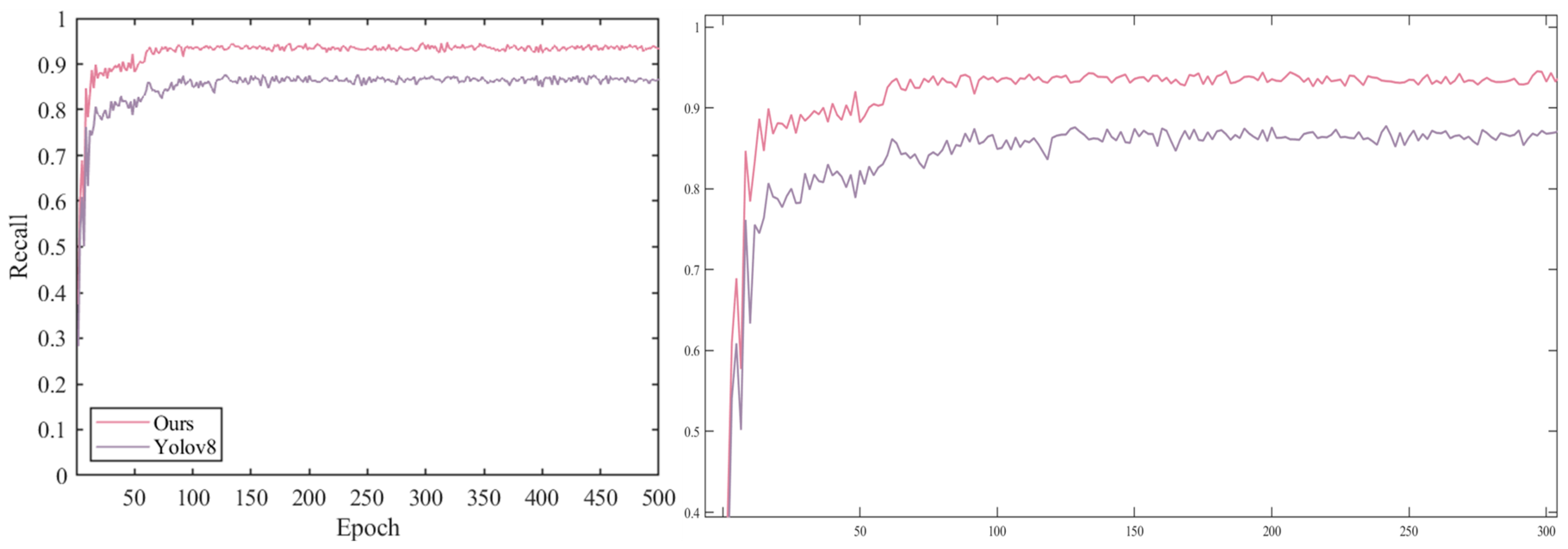
Figure 11 illustrates the comparison of recall performance between the model proposed in this paper and the original YOLOv8 during training. The analysis reveals that the proposed model outperforms the original YOLOv8 across all aspects, particularly in terms of recall, showcasing a substantial enhancement.

From 0 to 100 epochs, the recall of the improved model experiences a rapid increase, highlighting its ability to swiftly learn from the training data. In contrast, the recall of YOLOv8 shows a slower growth rate, indicating either a slower initial parameter optimization speed or suboptimal initial learning rate settings. In contrast, the improved model fully utilizes the SSA for learning rate optimization, yielding a significant advantage.

Between 100 and 200 epochs, the precision growth rate of the improved model decelerates and stabilizes, reaching a consistent level near 94.40%. Meanwhile, the precision of YOLOv8 gradually increases, but at a slower rate.

From 200 to 500 epochs, the precision of the improved model displays slight fluctuations but remains stable overall, possibly due to natural fluctuations in the model’s generalization performance resulting from the interplay between model complexity and training data. Conversely, the precision of YOLOv8 stabilizes around 91.55%, with a smooth precision curve, indicating stable adaptation of model parameters to the data during this stage.

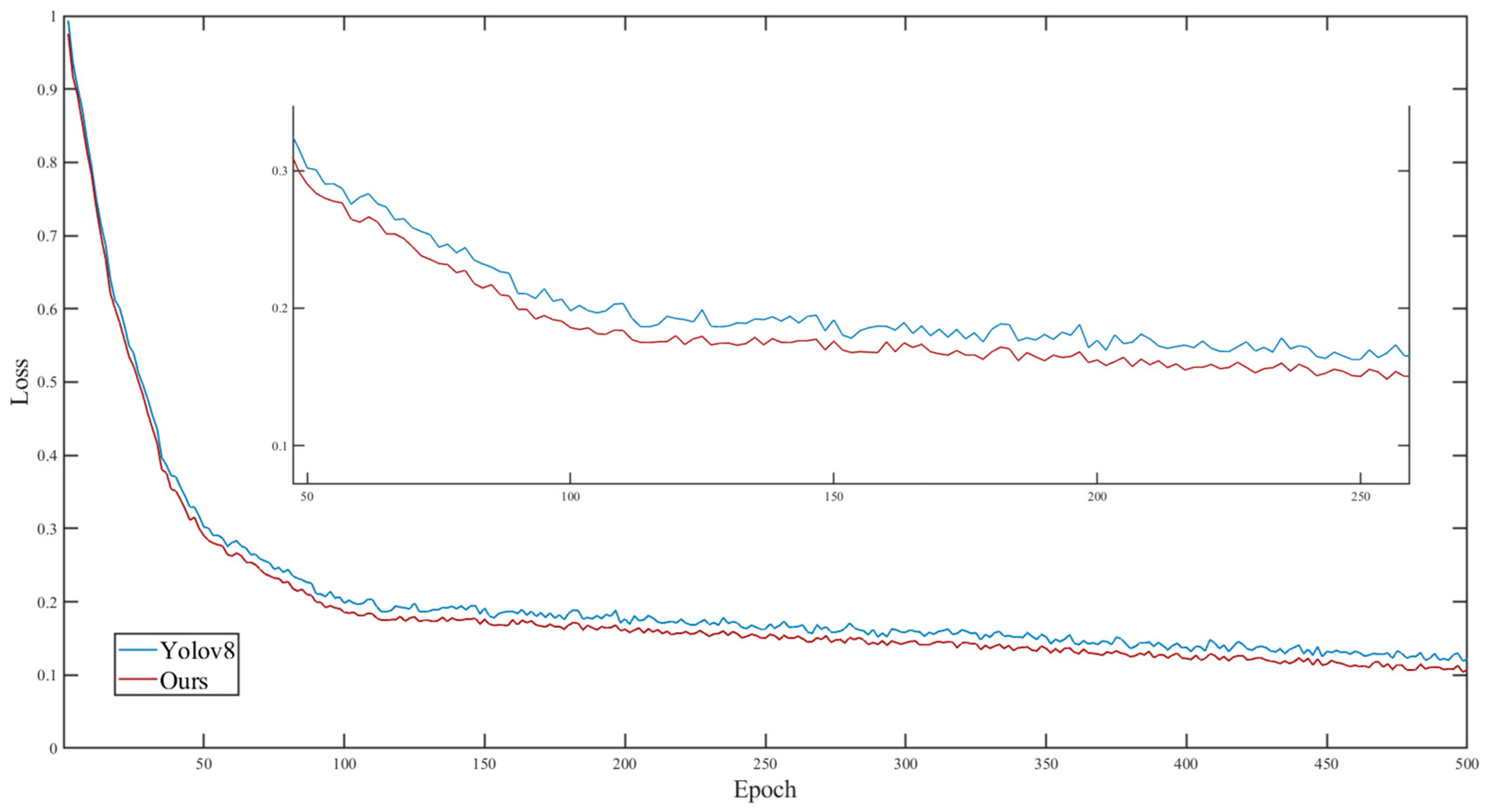
The graph in Figure 12 illustrates the comparison of the loss function (Loss) between the proposed model in this paper and the original YOLOv8 during the training process. Between 0 and 100 epochs, both models exhibit a sharp decrease in loss values, indicating their ability to rapidly learn from the training data. However, from epoch 100 to 200, the downward trend of the loss curve becomes smoother, suggesting a transition from rapid learning to finer optimization stages.

During this stage, the proposed model demonstrates slightly lower loss values than YOLOv8, indicating better learning efficiency or optimization strategy. This advantage may be attributed to the method used in the proposed model, which optimizes the learning rate using the SSA, thereby enhancing the effectiveness of the optimization process.

Between epochs 200 and 500, the loss curves of both models further stabilize, with minimal changes in loss values, indicating convergence of the models. The proposed model continues to maintain slightly lower loss than YOLOv8, underscoring its performance advantage throughout the training process.

The network model proposed in this paper has demonstrated significant performance improvements in maize tassel detection compared to the original YOLOv8 model. The precision (P) has increased by 3.27 percentage points to 97.59%, indicating higher accuracy in maize tassel recognition and effectively reducing false positives and false negatives. The recall rate (R) has increased by 2.85 percentage points to 94.40%, enabling more comprehensive detection of maize tassels in the images. The frames per second (FPS) increased from the original 37.92 to 40.62, allowing for faster completion of detection tasks, which is particularly important for real-time detection or large-scale data processing scenarios.

In terms of resource consumption, the new model also demonstrates advantages. The model parameter size (params) decreased from the original 16.52 MB to 14.62 MB, reducing the storage requirements of the model and facilitating deployment on resource-constrained devices. Additionally, the floating-point operations (GFLOPs) decreased from 12.31 to 11.21, reducing the computational complexity of the model and improving operational efficiency. These optimizations render the new model more practical and widely applicable in real-world applications, providing strong technical support for automated maize tassel detection.

5.3. Module Ablation Experiments

To better validate the impact of the improved modules [19] and their combinations on enhancing the original model’s performance, this paper designed ablation experiments for drones flying at a height of 5 m above the ground. The experimental results in

Table 1. Ablation experiment table for different modules. Notes: Ablation experiment table for four different modules: Pconv, ACmix, CTAM, and SSA.

Method	Pconv Module	ACmix Module	CTAM Module	SSA	P/%	R/%	FPS /S	Params /MB	GFLOPs
Yolov8	–	–	–	–	94.32	91.55	37.92	16.52	12.31
(A)	√	–	–	–	92.34	89.27	40.52	13.25	10.67
(B)	–	√	–	–	95.48	92.28	36.34	16.83	12.52
(C)	–	–	√	–	95.81	92.43	36.63	17.53	12.92
(D)	–	–	–	√	95.56	92.37	36.51	16.07	11.87
(E)	√	√	–	–	95.03	92.08	38.82	14.57	11.89
(F)	√	–	√	–	95.12	92.17	38.63	14.61	11.72
(G)	√	–	–	√	95.26	92.31	38.24	14.71	11.69
(H)	–	√	√	–	96.88	93.39	37.82	15.72	13.39
(I)	–	√	–	√	96.72	93.23	37.89	15.42	12.64
(J)	–	–	√	√	96.81	93.36	37.92	15.39	12.78
(K)	√	√	√	–	96.11	93.08	39.83	14.74	11.34
(L)	√	–	√	√	97.23	94.32	39.79	14.81	11.42
(M)	–	√	√	√	97.71	94.51	39.82	14.90	11.29
(N)	√	√	√	√	97.59	94.40	40.62	14.62	11.21

demonstrate that with the addition and combination of various improved modules, the model exhibits varying degrees of improvement in precision (P) and recall (R), along with different levels of reduction in FPS, parameter count, and GFLOPs.

Results of the ablation experiment for the Pconv module (Models A, E, F, G, K, L, N): By introducing the partial convolution module, the model’s parameter size and computational complexity were reduced. Params decreased by 3.27, 1.95, 1.91, 1.81, 1.78, 1.71, and 1.90 MB, respectively, averaging a decrease of 2.05 MB. GFLOPs decreased by 1.64, 0.42, 0.59, 0.62, 0.97, 0.89, and 1.10, respectively, averaging a decrease of 0.89. The average increase in FPS was 1.57. P increased by an average of 1.06%, while R increased by an average of 0.968%.

Results of the ablation rxperiment for the ACmix module (Models B, E, H, I, K, M, N): By introducing the ACmix module, the extraction of key features in the feature map was achieved, allowing for better capturing of subtle features of corn tassels, thus reducing false positives and false negatives. P increased by 1.16, 0.71, 2.56, 2.4, 1.78, 3.39, and 3.27%, respectively, averaging an increase of 2.18%. R increased by 0.73, 0.53, 1.84, 1.68, 1.53, 2.96, and 2.85%, respectively, averaging an increase of 1.73%. The average increase in FPS was 0.814. Params decreased on average by 1.26 MB. GFLOPs decreased on average by 0.27.

Results of the ablation rxperiment for the CTAM module (Models C, F, H, J, K, L, M, N): The introduction of the CTAM module employed an almost parameter-free attention mechanism to model channel and spatial attention [38], effectively integrating feature information from different scales and levels. This enabled the model to comprehensively understand the image content and enhance the recognition ability of corn tassels. P increased on average by 2.31%. R increased on average by 1.92%. The average increase in FPS was 1.1. Params decreased on average by 1.24 MB. GFLOPs decreased on average by 0.411.

Results of the ablation experiment for the SSA (Models D, G, I, J, L, M, N): The adoption of the SSA, based on the sparrow search algorithm for learning rate optimization, enhances the model’s robustness and precision. Given the variations in the morphology, size, and color of corn tassels due to factors such as variety and growth environment, the model needs strong generalization capabilities in order to handle various complex scenarios. The introduction of the SSA enables the model to better adapt to these changes, improving its robustness and accuracy. P increased on average by 2.37%. R increased on average by 1.95%. The average increase in FPS was 0.76. Params decreased on average by 1.38 MB. GFLOPs decreased on average by 0.46.

In addressing the specific task of detecting and counting corn tassels, our research proposes an optimized variant of the YOLOv8 model through systematic integration and testing of different modules. Our experimental results clearly demonstrate that each individual module—Pconv, ACmix, CTAM, and SSA—plays a crucial role in improving model performance. Moreover, they ensure or enhance detection accuracy, while reducing model complexity and increasing inference speed. These experiments not only prove the importance of integrating multiple technologies to improve corn tassel detection performance, but also provide important guidance and reference for the development of future agricultural vision detection systems. We hope that these findings will be recognized by peers and further explored and applied in subsequent research.

5.4. Model Horizontal Comparison

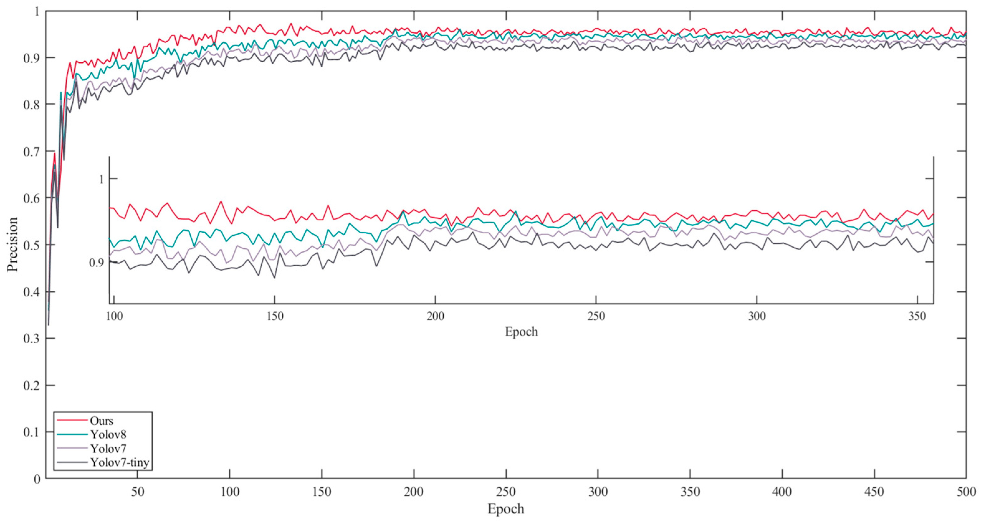
The line graph in Figure 13 illustrates the performance of four different models, namely the proposed model, Yolov8, Yolov7, and Yolov7-tiny, in terms of precision over 500 epochs. Precision is a crucial metric for assessing model performance. From the trend of the curves, it is observed that all models exhibit a rapid increase in precision during the initial stage (first 50 epochs), reflecting the models’ ability to quickly learn in the early stages of training. Subsequently, the improvement in precision starts to plateau, gradually stabilizing. This indicates that the models are converging and learning the key features of the dataset, namely the characteristics of maize tassels.

Among the four models compared horizontally, the proposed model consistently maintains the highest position, ultimately stabilizing around 97.59%, indicating that its precision across epochs is generally higher than in the other models. Yolov8 and Yolov7 exhibit similar performance, with curves closely aligned for most of the time, stabilizing at 95.83% and 95.57%, respectively. They demonstrate similar learning trends and performance levels. The precision of Yolov7-tiny remains consistently lower throughout the training process, stabilizing at 93.27%. This could be attributed to the simplified model structure of the “tiny” version, which is aimed at reducing computational complexity but results in decreased performance.

5.5. Comparison of Precision at Different Heights

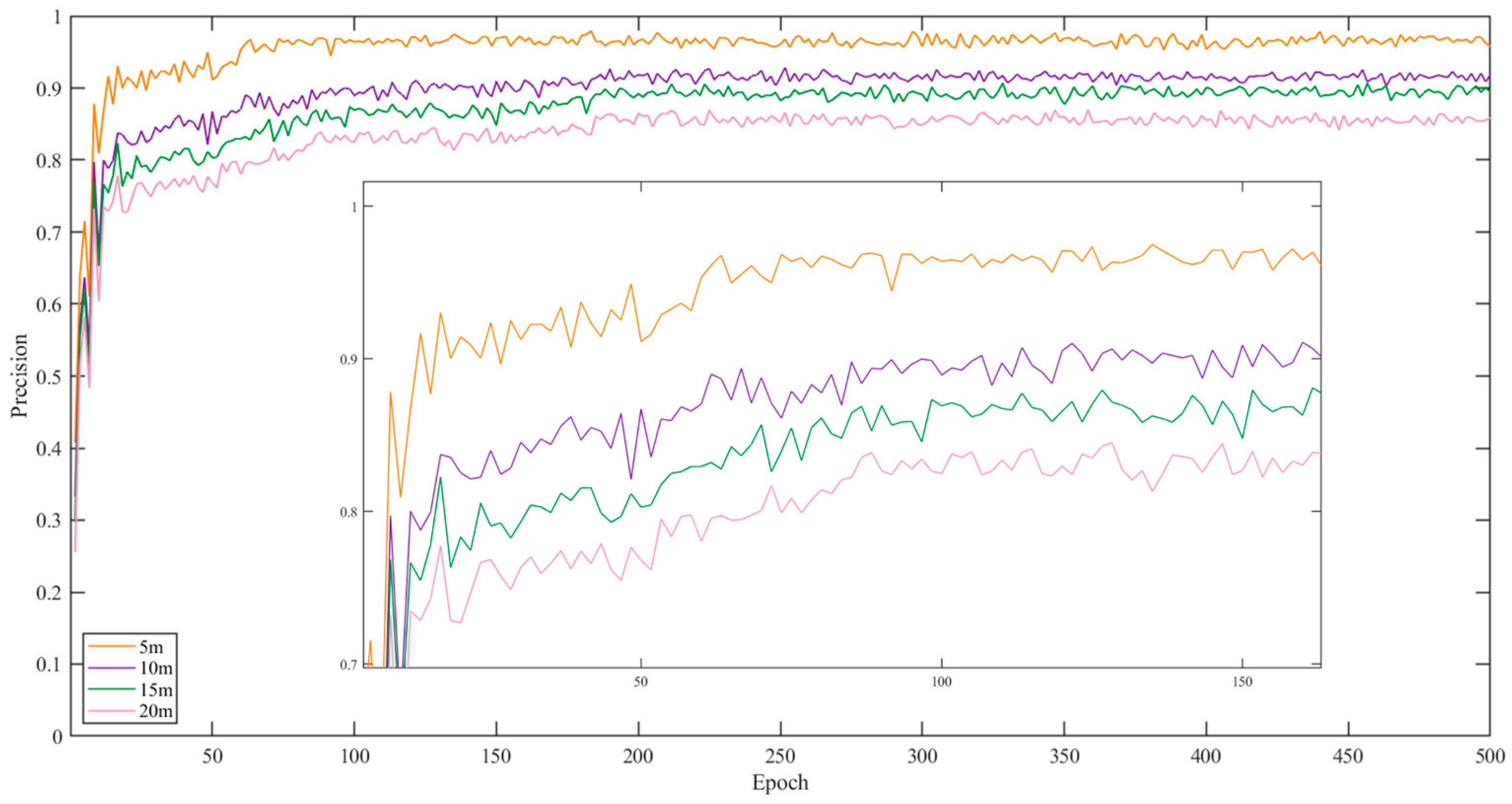
The graph in Figure 14 illustrates the line plot of model precision across 500 epochs under different altitude conditions. The orange line represents the model precision at a height of 5 m, the purple line represents the precision at a 10 m height, the green line represents the precision at a 15 m height, and the pink line represents the precision at a 20 m height.

During the initial epochs, the precision of models under all altitude conditions shows a rapid increase, indicating a quick improvement in predictive capability during the early stages of training. As training progresses, the growth in precision gradually slows down and stabilizes, indicating that the models are approaching convergence, and the learning gains diminish over time.

Among all conditions, the model’s precision is highest at height of 5 m, stabilizing at around 97.59%. This is attributed to the closer proximity and broader coverage, which favor accurate target prediction. In comparison, the precision of models at 10 m and 15 m heights is similar, stabilizing at around 90.36% and 88.34%, respectively, slightly lower than the precision under the 5 m condition, but higher than that under the 20 m condition.

The model’s precision is lowest at a height of 20 m, stabilizing at around 84.32%. This is due to the greater distance, resulting in decreased model performance.

5.6. Specific Detection Performance

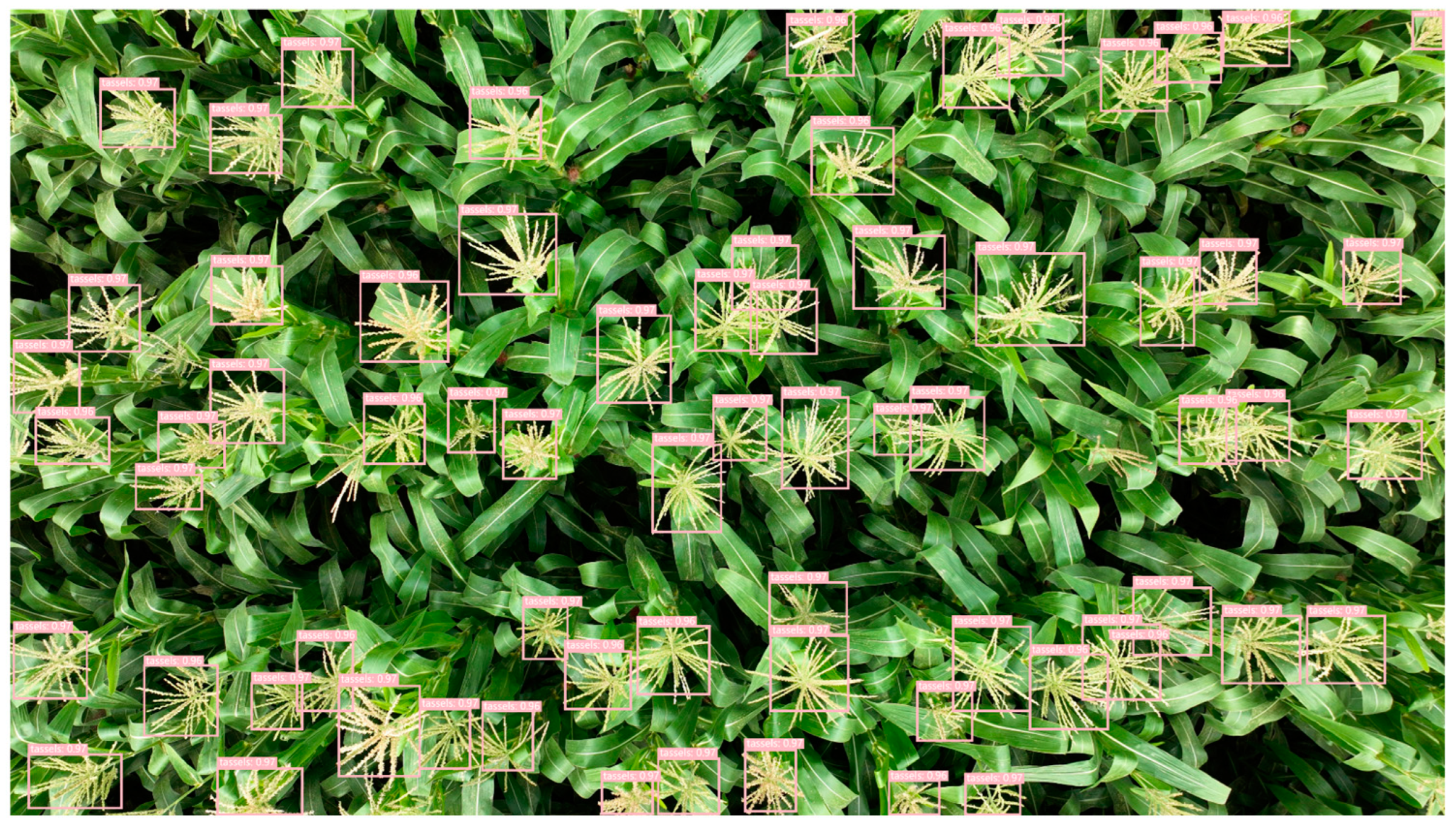
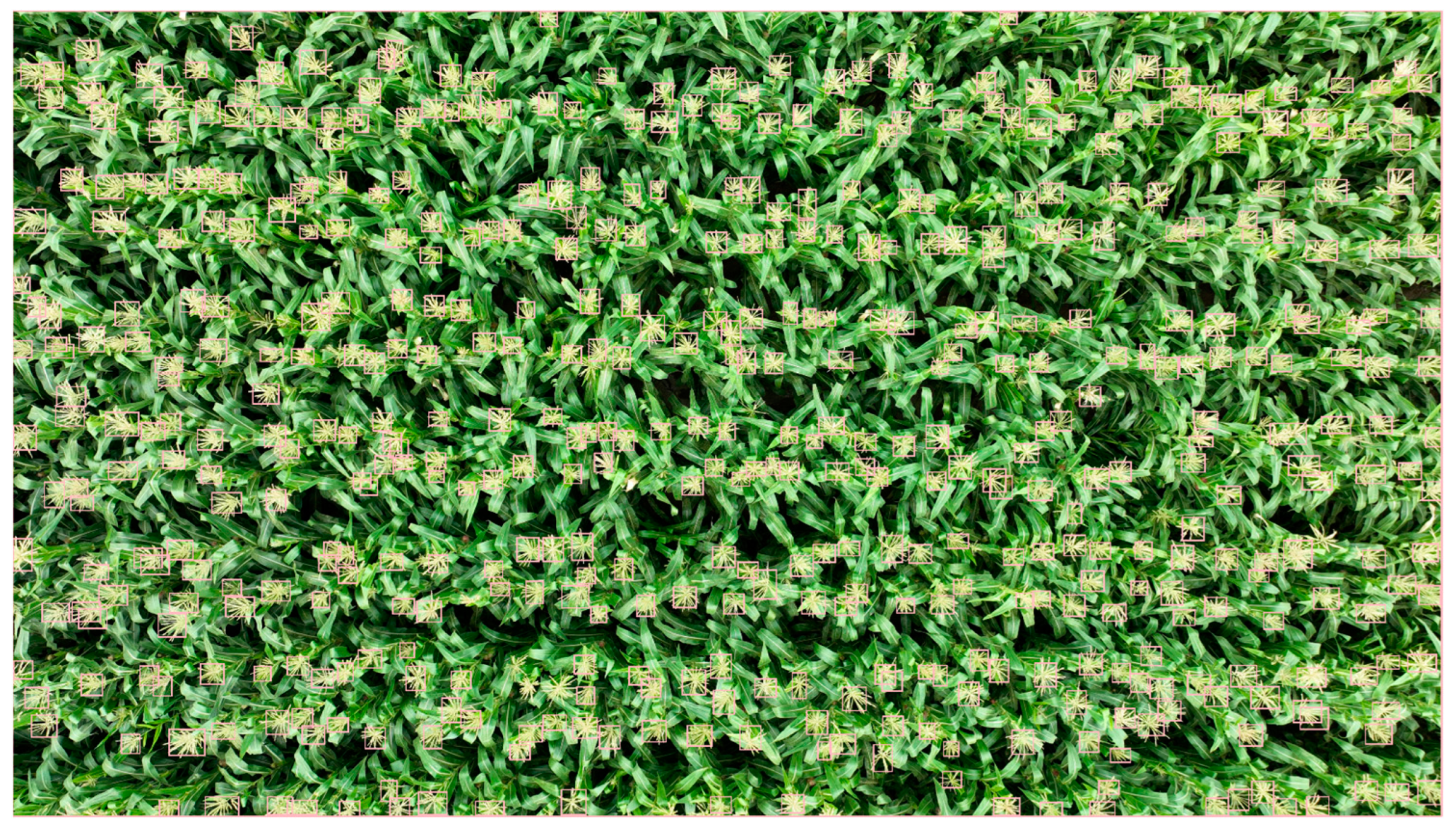
Figure 15 displays the detection results of maize tassels at a height of 5 m. It can be observed that most of the maize tassels are detected, and each bounding box is associated with a detection category and confidence score. Among the numerous bounding boxes of maize tassels, each has a high confidence score, indicating that the proposed algorithm can accurately identify the features of maize tassels.

Figure 16 displays the counting results of maize tassels at a height of 5 m. It can be observed that each maize tassel is accurately bounded, and a unique identifier is annotated on each bounding box, ensuring no duplication. This indicates an accurate count of maize tassels in the image.

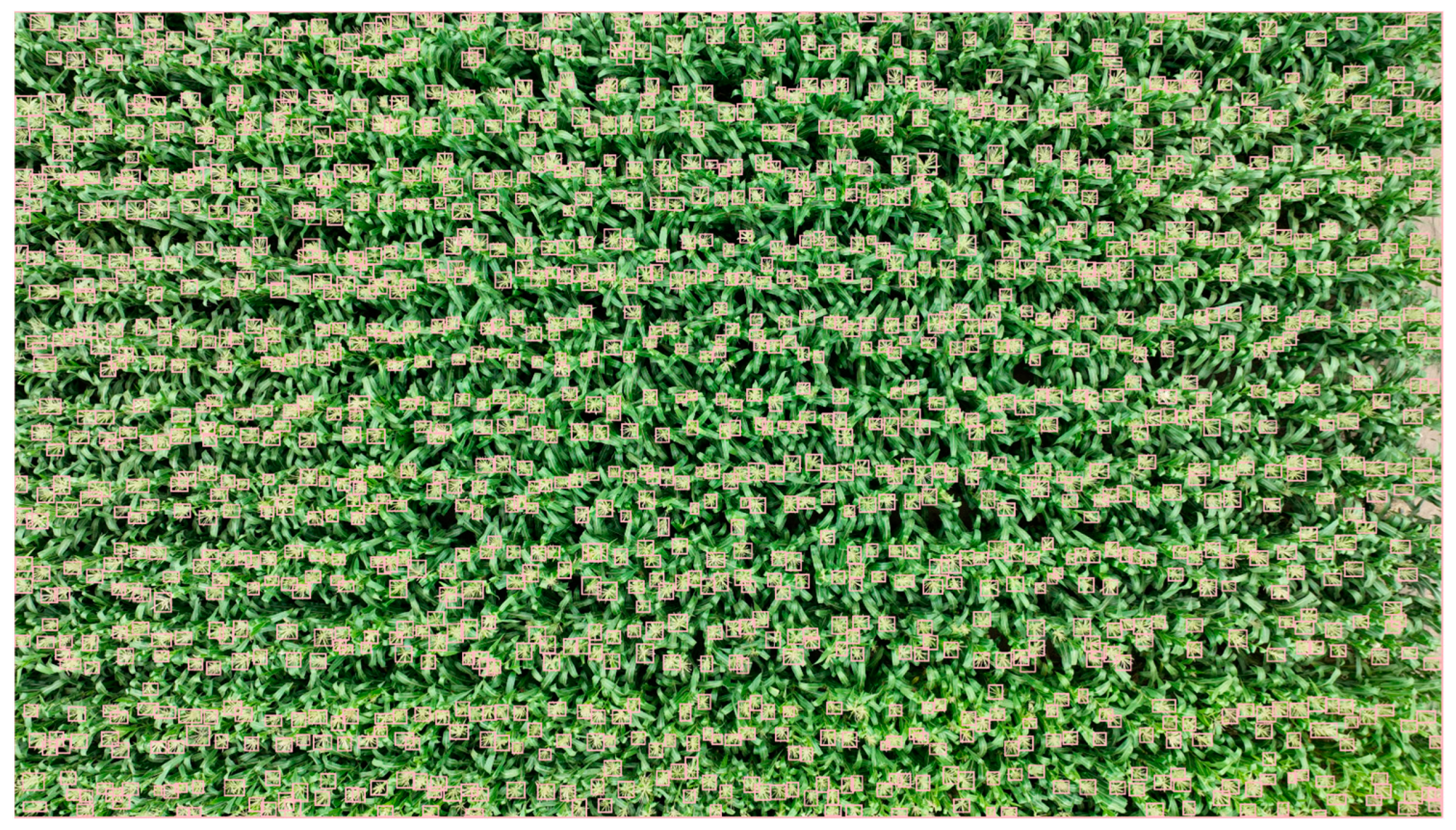
In Figure 17, the detection results of corn tassels at a height of 10 m are displayed. It is evident that most of the corn tassels are successfully detected, presenting clear and distinct detection outcomes.

On the other hand, Figure 18 illustrates the detection results of corn tassels at a height of 15 m. Despite the relatively small size of the corn tassels, the model adopted in this study, with a minimum detection feature map size of 20 × 20 × 512, is still capable of handling this task. However, the addition of another 10 × 10 detection head would pose challenges in terms of achieving a balance between precision, computational complexity, and multi-target detection.

6. Conclusions

Traditional research in corn tassel identification and counting has made significant strides, often leveraging drone imagery and deep learning algorithms such as CNN, Faster R-CNN, VGG, ResNet, and YOLO. However, one crucial aspect that is often overlooked is the impact of varying heights on identification and counting accuracy, as well as the performance metrics (P, R, FPS, params, and GFLOPS) of the models.

In recent years, the YOLO model has emerged as a prominent tool in computer vision. This study proposes utilizing YOLOv8 with drone imagery captured at different heights (5 m, 10 m, 15 m, 20 m) for corn tassel identification and counting. The investigation encompasses an evaluation of the model’s accuracy, computational complexity, and robustness under different altitude conditions.

In the original YOLOv8 model, we introduced the Pconv module to achieve lightweight design and faster detection speed. Within the backbone section, we incorporated the ACmix module, which combines the global perceptual ability of self-attention with convolution’s capability to capture local features. This integration enhances the model’s feature extraction capacity, particularly in the identification of corn tassels. Additionally, the CTAM module, integrated into the neck section, improves semantic information exchange between channels, ensuring precise and efficient corn tassel localization, while enhancing feature fusion capabilities. Finally, by leveraging the sparrow search algorithm (SSA) to optimize mean average precision (mAP), we enhanced the model’s robustness and detection accuracy [40].

The proposed network model demonstrates significant performance improvements in corn tassel detection, compared to the original YOLOv8 model, at a height of 5 m above the ground. Precision (P) increased by 3.27 percentage points to 97.59%, and the recall rate (R) increased by 2.85 percentage points to 94.40%. Moreover, the frames per second (FPS) increased from the original 37.92 to 40.62. The model’s parameter size (params) decreased from the original 16.52 MB to 14.62 MB, and the floating-point operations per second (GFLOPs) decreased from 12.31 to 11.21. Additionally, at heights of 10 m and 15 m above the ground, precision stabilized at around 90.36% and 88.34%, respectively, with the lowest precision observed at 20 m height, stabilizing at around 84.32%.

These optimizations render the new model more practical and widely applicable in real-world scenarios, offering robust technical support for automated corn tassel detection. Leveraging deep learning techniques and drone imagery for corn tassel recognition and counting presents convenient tools for agricultural practitioners to estimate crop yields and evaluate crop health status. This facilitates the advancement of modern agricultural technologies like agricultural IoT and smart agriculture, thereby propelling agricultural confirmedproduction towards intelligence and precision.