Go with the Flow: Estimating Wind Using Uncrewed Aircraft

Abstract

This paper presents a fundamentally different approach to wind estimation using Uncrewed Aircraft (UA) than the vast majority of existing methods. This method uses no on-board flow sensor and does not attempt to estimate thrust or drag forces. Using only GPS and orientation sensors, the strategy estimates wind vectors in an Earth-fixed frame during turning maneuvers. The method presented here is called the Wind-Arc method. The philosophy behind this method has been seen in practice, but this paper presents an alternative derivation with resulting performance evaluations in simulations and flight tests. The simulations verify the method provides perfect performance under ideal conditions using simulated GPS, heading angle, and satisfied assumptions. When applied to experimental flight test data, the method works and follows both the airspeed and wind speed trends, but improvements can still be made. Wind triangles are displayed at each instant in time along the flight path that illustrate the graphical nature of the approach and solution. Future work will include wind gust estimation and a Quality of Estimate (QoE) metric to determine what conditions provide good wind speed estimates while preserving the method’s generality and simplicity.

1. Introduction

Small uncrewed aircraft systems (sUAS) are providing access to the lower atmosphere in ways that have never before been possible. The prevalence and ease with which the lower atmosphere is accessible is revolutionizing aviation, weather observation, and atmospheric science. Colloquially referred to as drones, these small Uncrewed Aircraft (UA) are attractive across a broad range of applications, including the next generation of aviation [1], weather forecasting [2], atmospheric science [3,4], agriculture [5], medical transport [6], emergency response [7,8], law enforcement [9,10], surveillance [11], mapping and remote sensing for mining [12], archaeology [13,14,15], forestry [16,17], package delivery [4,18,19,20], and sustainable smart cities [21].

The usefulness of UA is clear, but associated regulations and procedures are not fully developed. The FAA’s and NASA’s work on both Uncrewed Traffic Management (UTM) and Advanced Air Mobility (AAM) is evidence of the future potential and challenges involved. To develop new regulations and procedures, the FAA must ensure safe flight enroute, and near vertiports, buildings, bridges, and other critical infrastructure. This is true for the current National Airspace (NAS) but also true for new air volumes near critical infrastructure that are added to the NAS. Wind plays (and will play) a critical role in flight around critical infrastructure, but wind is often (a) not measured and (b) more dynamic in these areas than in typical, open airspace. Seasonal and diurnal (time-of-day) variations around complex urban landscapes are difficult to predict. Additionally, small UA and future crewed aircraft will have less mass than most conventional aircraft.

Consequently, UA and AAM aircraft are more susceptible to wind and the environment in their intended flight locations. Thus, a lack of wind estimates in areas near infrastructure represents a critical safety risk to both UTM and AAM. This is not only a safety risk; it is a technology gap for both UTM and AAM. There are no low-cost, scalable methods for estimating wind in urban areas around buildings, bridges, trees, towers, and power lines.

What the FAA, NASA, and the aviation community needs is a broadly applicable, cost-effective, and scalable method for wind estimation using Uncrewed Aircraft. Uncrewed Aircraft can initially be flown in new, unexplored air volumes near critical infrastructure with greater safety for people and property than crewed aircraft. They will be the first air mobility presence in unchartered airspace to profile air volumes in preparation for greater use in the National Airspace. The method presented in this paper makes profiling buildings and high-wind areas more practical and scalable by commercial weather providers or individuals. The Wind-Arc method presented here can fill the technology gap in wind estimation near critical infrastructure for UTM and AAM.

1.1. Paper Organization

A broad survey of all commonly used wind estimation methods is presented below. Then, the two most prevalent approaches found in the literature are summarized. This provides context for this paper’s contribution: a third approach. Also, a lesser-known reference is presented that the authors believe is the first occurrence of this third method but is not presented in the literature base. An alternative formulation is presented with simulations, flight tests, and a comparison with a flow sensor-based method. The novel contributions of this paper are situating the lesser-known references within the literature base, formulating an alternative, more straightforward derivation, presenting the method’s simulation-based verification under ideal conditions, and direct comparison to a flow sensor-based approach using two separate instrumented vehicles. Also, illustrations of wind triangles at specific points along the flight path reveal both the GPS velocities in sequence and the resulting airspeed and wind speed solutions. These wind triangle sequences reveal the variable nature of wind and provide clues to the method’s accuracy along the flight path.

1.2. Broad Survey of Wind Estimation Methods

A fairly complete summary of wind velocity measurements is described below that span different communities of practice. The aviation community is interested in only as much accuracy as needed to safely fly aircraft. Measuring the direction and approximate magnitude is sufficient. An aviator’s approach can be as simple as dropping blades of grass at an airfield to see which way they fall or how fast they fall. Where a wind-sock is available, aviators are trained to estimate the prevailing wind speed and direction using a wind-sock [22,23]. Also, anemometers are referenced from ground-based weather stations, which can, sometimes, be an appreciable distance away. These readings are helpful but sometimes are not close enough to the flight area to be useful. This is one of the primary motivators for hyper-local wind estimation. Pitot tubes are the most common method for estimating airspeed while in flight. A method used by early aviators to estimate wind and direction is called ‘the circle’, the ‘wind drift circle’ [24,25], or the ‘turns around’ method. The weather community uses anemometers for stationary measurements at weather stations or meteorological towers. Newer weather stations typically use sonic anemometers, whereas earlier stations used cup-type. Meteorological towers and wind LiDAR are both designed to provide vertical wind profiles. The tower requires more infrastructure than a ground-based wind LiDAR but often provides superior measurements. Wind farm profiling, rocket launches, and profiling winds near buildings and bridges are use-cases that need this type of wind monitoring [26,27,28,29,30]. In NASA flight tests, a smoke tower was used to visualize turbulent vortices generated by a passing aircraft [31,32,33,34]. These studies helped inform FAA take-off spacing times. Mobile wind measurements for weather prediction also include dropping radiosondes or launching weather balloons [35]. The atmospheric science community uses all of these methods but typically relies on 2D or 3D sonic anemometers. Engineers and scientists can use multi-hole pressure probes (MHPPs) [36], hot-wire anemometry [37], Particle Image Velocimetry (PIV) [38], or Particle Tracking Velocimetry, depending on the application. Engineers and aerodynamicists in the aviation and racecar communities use CFD simulations, smoke-streams in wind tunnels, or tufts of yarn attached to a wing or an airfoil. The most accurate method used by the National Institute for Standards and Technology (NIST) is called a Laser Doppler Anemometer (LDA) [39]. In 2010, NIST replaced Pitot tubes with Laser Doppler Anemometers because Pitot tubes require air properties while LDA measurements are entirely mechanical, and thus, traceable to the U.S. National standards of length and time [40]. LDA can measure flows as slow as blood movement in blood vessels and as high as rocket exhaust velocities nearing 1000 m/s.

2. Literature Review

There are two broad, well-established approaches in the literature for wind estimation using drones. This section discusses these two methods, and then, presents a unique third method.

2.1. Approach 1: Direct Flow Measurement Using On-Board Flow Sensors

By mounting an air flow measurement device on an Uncrewed Aircraft, the vehicle’s airspeed can be estimated directly. This is a direct flow measurement in the body-fixed vehicle frame. Direct flow measurement can be performed using any sensor that is compact and light enough to fit the aircraft’s payload capacity. There are several on-board flow sensor options, but, in practice, only two types are commonly seen on UA: pressure sensors and sonic anemometers.

2.1.1. Pressure-Based Pitot Tubes or MHPPs

Pressure-based flow sensors measure static and total air flow pressure and directly relate it to speed. Single-hole Pitot tubes produce a one-dimensional wind measurement along the axis of the tube, as demonstrated by Arain [41]. MHPPs use the same concept but, with additional holes, are able to produce 2D or 3D wind vector measurements. The vehicles from De Boer [42], shown in Figure 1, and Van den Kroonenberg [43] are examples of MHPPs. Pressure flow sensors, however, can only measure the sensor’s facing direction. This concept is well suited for fixed-wing aircraft, but multi-rotors have more complex six-degree-of-freedom motion. The ability for omnidirectional motion, plus associated rotor wash [41], makes it difficult to incorporate a directional-based sensor like a Pitot tube or MHPP on a multi-rotor UA.

2.1.2. Ultrasonic Anemometers

Ultrasonic Flow sensors are commonly seen in two types: Time-of-Flight (Tof) and Acoustic Resonance [44,45]. Time-of-flight sensors relate wind speed to the measured time for an ultrasonic pulse to travel from an emitter to a receiver. The air flow influences pulse speed, and both 2D and 3D correlations are effectively achieved using sonic anemometers. The second sensor type, used in this work, is an Acoustic Resonance (Acu-Res^®) FT205 with a patented method [21] to measure wind speed and direction independent of air temperature and pressure. Ultrasonic anemometers are typically seen on multi-rotor UA, like Shimura’s setup [46] in Figure 1, and other published field campaigns [47,48]. Mounting these sensors on fixed-wing UA sometimes adds complications by changing the vehicle’s center of gravity and flight characteristics, along with the necessary consideration given to sensor placement.

Figure 1. Instrumented UA with on-board flow sensors: (a) Multi-rotor with sonic anemometer on mast [46]; (b) eVTOL fixed-wing aircraft with a nose-mounted Multi-Hole Pressure Probe (MHPP) and Pitot Probe [42].

Figure 1. Instrumented UA with on-board flow sensors: (a) Multi-rotor with sonic anemometer on mast [46]; (b) eVTOL fixed-wing aircraft with a nose-mounted Multi-Hole Pressure Probe (MHPP) and Pitot Probe [42].

Pressure-based or ultrasonic sensors ideally arrive pre-calibrated from the factory. Neither has any moving parts, which is ideal. But there is a cost penalty associated with high-quality anemometers. Prices range from USD 1500 to over USD 20,000 and any calibration adds to the operational complexity and cost.

2.1.3. Mounting and Flight Considerations

The greatest challenge with the flow sensor method is ensuring that the sensor is sufficiently far enough away from the rotor-induced flow field to measure representative ambient air. Also, sensor mounting needs to include power and a signal for data logging. The on-board sensors measure airspeed. To measure wind, vehicle velocity must be subtracted. The wind triangle relationships presented later in this paper typically use an Earth-fixed frame, such as North-East-Down (NED). Since measurements are in the body-fixed frame, the transformation from the body-fixed frame to the NED frame requires vehicle orientation, which is another three or four floating point numbers. So, subtracting vehicle speed from the airspeed measurement seems conceptually straightforward but is difficult in practice. In addition to this challenge, the incorporation of any specialized mechanical or electrical sensor requires additional pre-flight attention, and the sensor payload will either reduce power from the vehicle’s mobility battery directly or require additional payload for an instrumentation battery. It may be possible to incorporate data collection into a flight controller, but this has specifically been avoided with our research platforms to avoid any possibility of interfering with UA command and control (C2).

Our research group has successfully measured airspeed with multiple MHPP devices and multiple sonic anemometers. This includes subtracting vehicle velocity for atmospheric field investigations [49], wind estimation in urban canyons [3,4], and wind prediction from the middle of a prescribed fire [50].

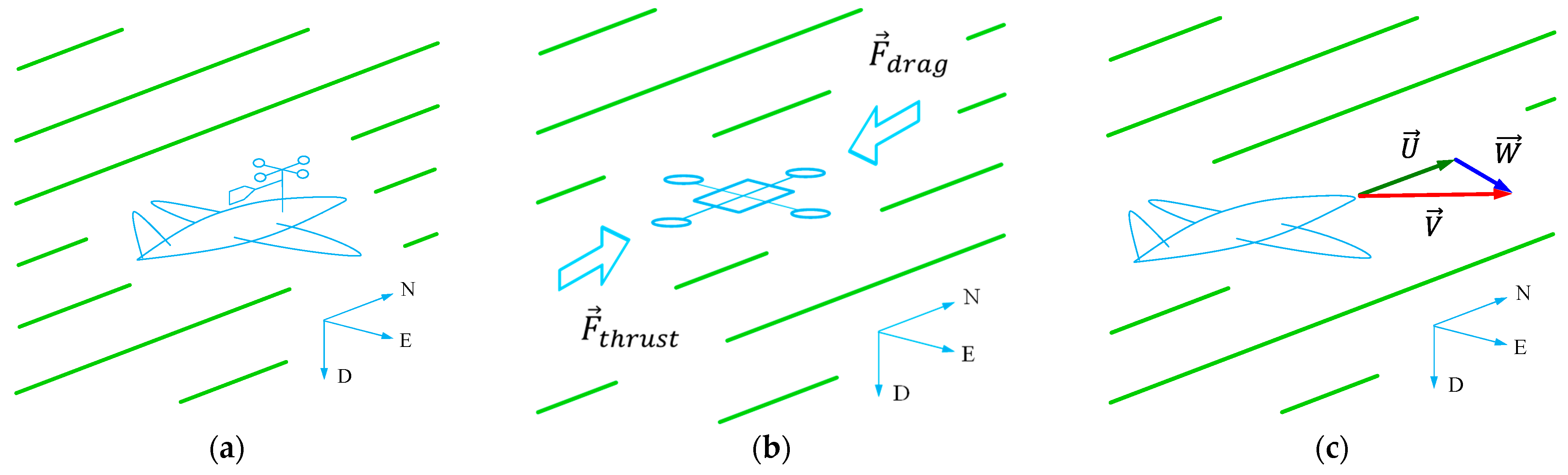
2.2. Approach 2: Thrust and Drag Force Estimation While Rejecting Wind

The second wind estimation approach in the literature relies on estimating vehicle thrust and drag forces during some type of prescribed flight path. If the vehicle is stationary (hovering), such as with multi-rotors, this method is also referred to as the “tilt angle” or “tilt” method. The assumption is that the on-board flight controller will reject wind disturbances effectively. The compensation required to reject these disturbances can be related to the magnitude and direction of wind acting on the UA. DJI multi-rotor flight controllers can provide wind speed estimates during flight, over the flight telemetry channel. This is helpful, but the wind estimation accuracy and method are both unknown because DJI provides a proprietary, closed-source ecosystem.

2.2.1. Classical Dynamic Modeling Approach

Some methods estimate thrust and drag forces by leveraging the sophisticated on-board flight controllers with high-speed feedback loops and hard real-time operating systems. With known thrust and drag force estimates, and the drone’s windward frontal area, the wind direction and velocity can be estimated. These wind estimation methods are sophisticated, effective, and non-trivial. A survey of these methods is listed here [48,51,52,53,54]. These methods include clever approaches to characterizing motor and rotor thrust and monitoring the flight controller response signals, and can even estimate mass distribution on-board, in real time. Abichandani [53] and Palomaki [48] both conducted a comparative analysis between the flow sensor method and force estimation method.

2.2.2. Machine Learning Method

Certain quantities in the classical dynamics modeling approach are hard to measure and obtain. Examples include controller-specific gains used to reject wind disturbances, rotor speeds for a thrust measurement, and the wind-facing frontal area and drag coefficients. Machine Learning (ML) approaches have seen an increase in popularity, specifically for estimating these difficult quantities. Both Allison [55] and Wang [56] use different forms of ML to make wind predictions. Though their results look promising, a major drawback of this form of estimation lies with the generated ML model. These models are very specific to the trained vehicle and are not effectively usable across a variety of different platforms. These strategies are also not used for real-time predictions.

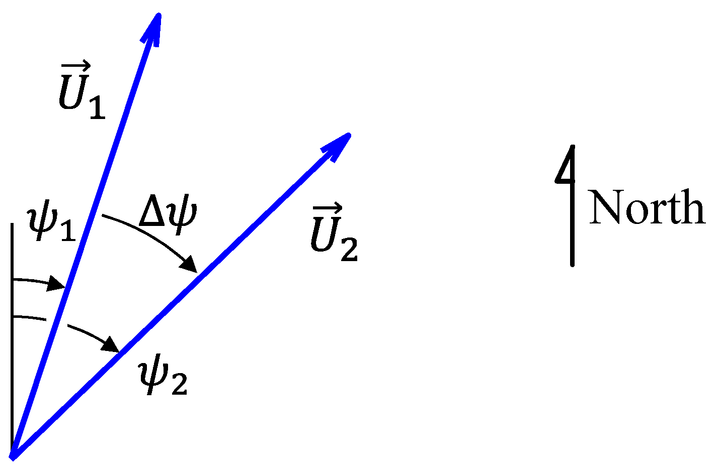
3. The Wind-Arc Method: Go with the Flow

Approach 1 described above needs on-board flow sensors. Approach 2 estimates thrust and drag force while the flight controller rejects wind as a disturbance. The third method highlighted here uses no flow sensor and has an entirely different basis than Approach 2. Instead of rejecting wind as a disturbance, this method seeks maximal influence from the wind, hence the phrase “Go with the Flow”. Conceptually, it is quite similar to the aviator’s wind drift circle method, except that it does not require an entire circle to be flown. This is called the Wind-Arc method because it is an abbreviated or fractional version of the aviator’s wind drift circle.

To the best of our knowledge, this approach was originally developed by a researcher named Dr. William Premerlani and presented on a drone enthusiast forum called DIYDrones.com in a post titled “Wind estimation without an airspeed sensor” [57]. The post described a new approach to 3D sensorless wind estimation with some benefits and limitations. The post included a white paper reference describing the algorithm in more detail [58]. There is another related white paper that somewhat addresses wind estimation but is more focused on a new flight control approach [59]. Dr. Premerlani is a published researcher in other areas, but neither the DIYDrones.com forum post nor the white paper [58] are indexed in the formal literature base.

One 2012 paper by Mayer et al. presents a similar concept of a ‘no-flow-sensor’ Wind Estimation Algorithm using multiple samples while turning [60]. A minimization routine seeks to minimize a cost function that fits a circle through measured GPS points. The approach is similar to Premerlani’s work with wind triangles during turning. But differences exist from use of an optimization routine with $N$ points rather than two successive points. The 2012 paper uses simulation to investigate time-based or spatially based sampling methods. The authors also perform real flights with a fixed-wing drone using the Paparazzi flight controller with favorable results. This is the same flight control software that Premerlani used to evaluate the method presented in the previous references. The 2012 paper’s work has value in combination with the current approach presented.

Both Premerlani’s work and the Mayer paper do not use a flow sensor, so they are not Approach 1. They also do not estimate thrust or drag while rejecting wind as a disturbance, so they are not Approach 2. This approach, specifically by Premerlani, represents an entirely different class of wind estimation that solves for the wind vector at two times, $t_1$ and $t_2$, using successive wind triangle relationships during turning. Illustrations of the three approaches are shown in Figure 2. Because it functions while turning but does not require a complete circle, it is a fractional circle, or arc. This is the origin of the Wind-Arc name. The method assumes that vehicle airspeed and wind speed remain constant between the two sensor snapshots at $t_1$ and $t_2$. It works by detecting small vehicle heading changes, ${\psi }_1$ and ${\psi }_2$, and combines these with GPS velocity vectors, ${\overrightarrow{v}}_1$ and ${\overrightarrow{v}}_2$, at each heading. Using these, plus the constant wind assumptions, the 2D or 3D wind vector, $\overrightarrow{W}$, can be solved algebraically. The three broad approaches summarized in this section are illustrated below.

3.1. Wind-Arc Derivation

The authors find no obvious flaws in the formulation presented in [58] but the derivation is dense. Also, there is a claim of 3D generality, which, for the most part, is acceptable. But 3D solutions from only pitching motion are not fully substantiated. The formulation presented here has the same generality and is an alternative, more straightforward development. The Wind-Arc method uses the wind triangle at two separate instances to algebraically solve for the wind vector using constant wind and constant airspeed assumptions. The wind triangle is a well-known vector relationship between vehicle ground speed, airspeed, and wind vectors:

$$\overrightarrow{V}=\overrightarrow{U}+\overrightarrow{W}$$

(1)

where $\overrightarrow{V}$ is the vehicle’s ground speed vector, $\overrightarrow{U}$ is the vehicle’ airspeed vector, and $\overrightarrow{W}$ is the wind speed vector. In this paper, all vectors are expressed in Earth-fixed North-East-Down (NED) coordinates. Also, the wind triangle and this formulation are valid for 3D vectors, but only 2D vectors are presented for clarity. For an aircraft maneuvering from heading 1 to heading 2, the wind triangle is illustrated below. The airspeed vectors ${\overrightarrow{U}}_1$ and ${\overrightarrow{U}}_2$ are identical in magnitude between Figure 3a, but are rotated by a small angle, $\Delta \psi$, from ${\psi }_1$ to ${\psi }_2$. The wind vectors ${\overrightarrow{W}}_1$ and ${\overrightarrow{W}}_2$ are identical in 1 and 2.

The heading change is defined in Equation (2), which represents an orientation change relative to 1.

$$\Delta \psi ={\psi }_2-{\psi }_1$$

(2)

Figure 3 illustrates the concept of successive wind triangles separated by $\Delta \psi$.

The wind triangles at 1 and 2 in Figure 3 capture this heading change. For states 1 and 2, the wind triangle relationships are both true at each instant, and thus, represent two independent equations:

$${\overrightarrow{V}}_1={\overrightarrow{U}}_1+{\overrightarrow{W}}_1$$

(3)

$${\overrightarrow{V}}_2={\overrightarrow{U}}_2+{\overrightarrow{W}}_2$$

(4)

The ground speed vectors $\overrightarrow{V_1}$ and $\overrightarrow{V_2}$ are directly measurable by GPS. The airspeed vectors $\overrightarrow{U_1}$ and $\overrightarrow{U_2}$ and wind vectors $\overrightarrow{W_1}$ and $\overrightarrow{W_2}$ are all unknown. By comparing successive measurements between heading angles ${\psi }_1$ and ${\psi }_2$, and assuming the airspeed magnitude and wind vectors remain constant during this brief period, the wind triangles in Equations (3) and (4) represent two independent equations, which allows for a solution of both $\overrightarrow{U}$ and $\overrightarrow{W}$ at instants 1 and 2. The assumptions for constant airspeed and wind speed are:

$$\left|{\overrightarrow{U}}_1\right|=\left|{\overrightarrow{U}}_2\right|$$

(5)

$${\overrightarrow{W}}_1={\overrightarrow{W}}_2$$

(6)

Rearranging (3) and (4) to express ${\overrightarrow{W}}_1$ and ${\overrightarrow{W}}_2$ explicitly in the NED frame gives the following:

$${\overrightarrow{W}}_1={\overrightarrow{V}}_1-{\overrightarrow{U}}_1$$

(7)

$${\overrightarrow{W}}_2={\overrightarrow{V}}_2-{\overrightarrow{U}}_2$$

(8)

Assuming the wind is constant during the short period between points 1 and 2, this allows the wind vectors to be solved algebraically. Relating (7) and (8) with (6) results in the following:

$${\overrightarrow{V}}_1-{\overrightarrow{U}}_1={\overrightarrow{V}}_2-{\overrightarrow{U}}_2$$

(9)

Remembering that these are still vector relationships in the Earth-fixed NED frame and that $\overrightarrow{V_1}$ and $\overrightarrow{V_2}$ are measurable using GPS, what is needed now is a way to relate the two airspeed vectors between points 1 and 2.

3.2. Alias and Alibi Transformations

There are two unknown airspeed vectors in Equation (9): ${\overrightarrow{U}}_1$ and ${\overrightarrow{U}}_2$. Equation (5) states that the magnitudes of these airspeed vectors are approximately the same, but their directions can be different because the vehicle turns from heading 1 to heading 2. This is illustrated in Figure 4.

This may seem a straightforward application of a 2 × 2 transformation matrix, and it is. But there is a subtle, yet important, difference that is critical to arriving at a correct solution. In robotics and dynamics, a common need is to express the same vector in a new or different coordinate frame. This is called a passive or alias transformation. This is illustrated with the unit vector $i$ and $j$ components of frames 1 and 2:

$$\left[\begin{array}{c}{\widehat{i}}_2\\ {\widehat{j}}_2\end{array}\right]=T_{\Delta }·\left[\begin{array}{c}{\widehat{i}}_1\\ {\widehat{j}}_1\end{array}\right]\mathrm{where}{T}_{\Delta }=\left[\begin{array}{cc}c\Delta \psi & s\Delta \psi \\ -s\Delta \psi & c\Delta \psi \end{array}\right]$$

(10)

But what is needed to solve Equation (9) is an active or alibi transformation, because ${\overrightarrow{U}}_2$ represents a different vector in the same NED coordinate frame. Using identical terminology as in (10) illustrates the difference:

$$\left[\begin{array}{c}{\widehat{i}}_2\\ {\widehat{j}}_2\end{array}\right]=T_{\Delta }^T·\left[\begin{array}{c}{\widehat{i}}_1\\ {\widehat{j}}_1\end{array}\right]\mathrm{where}{T}_{\Delta }\mathrm{is}\mathrm{defined}\mathrm{above}$$

(11)

The only difference between Equations (9) and (10) is the transpose operator. Now, ${\overrightarrow{U}}_2$ can be expressed as a function of ${\overrightarrow{U}}_1$ and the small heading change, $\Delta \psi$, with the alibi transformation:

$${\overrightarrow{U}}_2=T_{\Delta }^T·{\overrightarrow{U}}_1$$

(12)

Inserting (12) into (9) and rearranging yields the airspeed vector, ${\overrightarrow{U}}_1$, as a function of GPS velocities at points 1 and 2 and the orientation change, $\Delta \psi$:

$${\overrightarrow{U}}_1=N^{-1}·\left[{\overrightarrow{V}}_2-{\overrightarrow{V}}_1\right]$$

(13)

where $N=T_{\Delta }^T-I$ and $I$ is the 2 × 2 identity matrix. Equation (13) estimates the airspeed using only ground velocity vectors from two GPS readings and the associated heading angles, which are easily obtainable from an orientation sensor. The only two assumptions incorporated are constant airspeed magnitude and constant wind vectors between points 1 and 2. A related condition is that the change in heading angle must be large enough to ensure matrix $N$ has a well-conditioned inverse. The inverse of $N$ will exist for all $\left|\Delta \psi \right|>{\Delta \psi }_{thresh}$. Choosing ${\Delta \psi }_{thresh}$ between 1 and 10 degrees provides a well-conditioned inverse for $N$, even with real sensors and associated errors. The heading angle change can be larger than 10 degrees, but this risks more sensor snapshots between points 1 and 2 that violate the constant wind and airspeed assumptions compared to a smaller angle change threshold. So, the lower bound is preferred as long as $N^{-1}$ is well conditioned. Capturing wind estimates as quickly as reasonable also provides a higher frequency of estimates that can help deduce true wind speed despite non-constant winds (i.e., invalid assumptions) during some 1–2 snapshots.

Now, with the airspeed ${\overrightarrow{U}}_1$ known, and ${\overrightarrow{U}}_2$ from (12), the wind vectors can be solved algebraically. Inserting (13) into (7) yields:

$${\overrightarrow{W}}_1={\overrightarrow{V}}_1-N^{-1}·\left[{\overrightarrow{V}}_2-{\overrightarrow{V}}_1\right]$$

(14)

and inserting (12) and (13) into (8) yields:

$${\overrightarrow{W}}_2={\overrightarrow{V}}_2-T_{\Delta }^T·N^{-1}·\left[{\overrightarrow{V}}_2-{\overrightarrow{V}}_1\right]$$

(15)

Common GPS receivers provide speed and Course Over Ground (COG) directions, both of which are scalars. The ${\overrightarrow{V}}_1$ and ${\overrightarrow{V}}_2$ vectors can be assembled from GPS speed and COG using:

$$\overrightarrow{V}=\left[\begin{array}{c}GPSspeed·\mathrm{c}\mathrm{o}\mathrm{s}\left(COG\right)·\widehat{I}\\ GPSspeed·\mathrm{s}\mathrm{i}\mathrm{n}\left(COG\right)·\widehat{J}\end{array}\right]$$

(16)

Care must be taken when converting GPS speed and COG into SI units. GPS speed is often reported in knots and Course Over Ground reported in degrees on [0, 360]. The $\widehat{I}$ and $\widehat{J}$ vectors represent NED directions in the northing and easting directions, respectively, as shown in Figure 5. North corresponds to the $+X$ axis and east corresponds to the $+Y$ axis.

4. Results in Simulation

The value of simulation for a wind estimation algorithm cannot be overstated. Wind, by its very nature, is unpredictable and is rarely constant for more than brief moments. Simulation can provide idealized wind vectors or fields that are constant or change predictably to verify algorithm effectiveness in different scenarios. A simple kinematic vehicle model called the Dubins Airplane was used to model fixed-wing aircraft motion and turning [61,62]. The kinematic model has no forces or moments and describes 3D motion given a forward velocity, $V$; vertical climb rate input, $u_z$; and roll angle, $\varphi$, for turning. The model is similar to Dubins’ Car but modified to model a fixed-wing aircraft. The kinematic equations of motion in the Earth-fixed, $XYZ$, frame are given in [62].

$${\overrightarrow{v}}_g^{XYZ}={\left[\begin{array}{c}V·\cos \left(\psi \right)·\cos \left(\gamma \right)\\ V·\sin \left(\psi \right)·\cos \left(\gamma \right)\\ u_z\end{array}\right]}^{XYZ}$$

(17)

Steering is achieved by specifying a roll angle, $\varphi$, that generates the vehicle yaw rate:

$$\dot{\psi }=\left(g/V\right)·\mathrm{t}\mathrm{a}\mathrm{n}\left(\varphi \right)$$

(18)

where $g$ is gravity. The glide path angle is defined as $\gamma =\mathrm{a}\mathrm{r}\mathrm{c}\mathrm{t}\mathrm{a}\mathrm{n}(u_z/V)$.

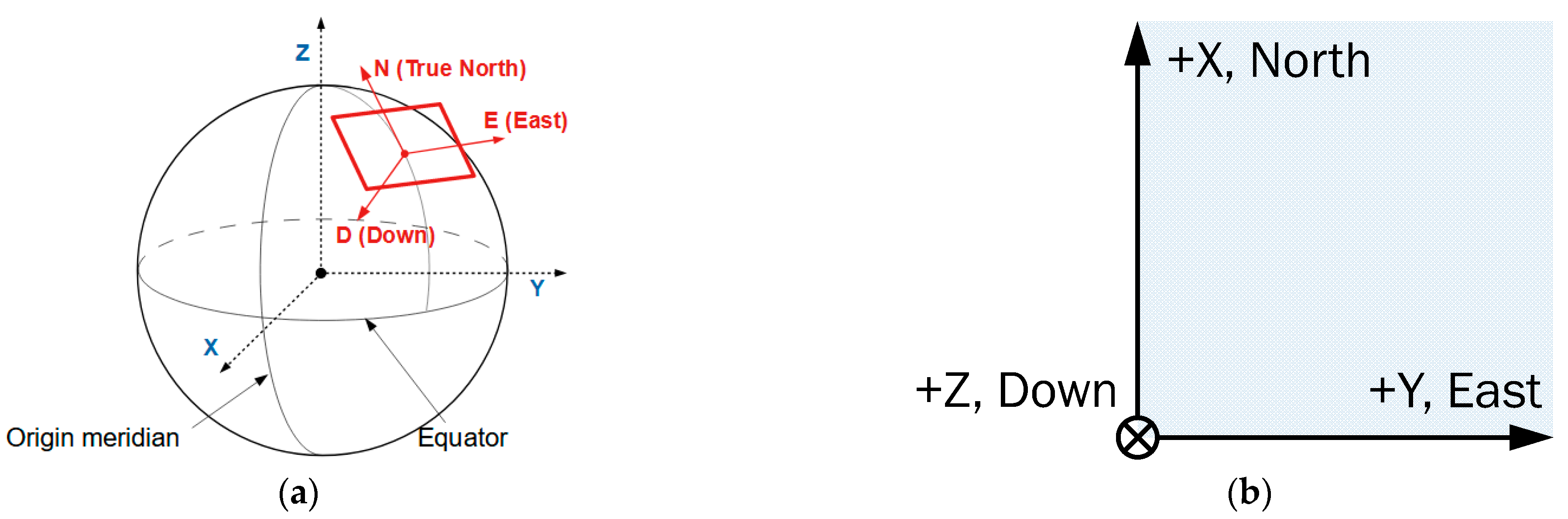
4.1. Coordinate Frames for Vehicle Dynamics and the Wind Triangle

Care must be taken to keep track of different coordinate frames and terminologies among the dynamics, weather, aviation, and atmospheric science communities. Three coordinate frames are involved in simulation and the associated experimental data: Cartesian XYZ, NED, and Universal Transverse Mercator (UTM).

To model vehicle motion in the presence of wind, the vehicle motion equations above need an additional term to create the previously established wind triangle, $\overrightarrow{V}=\overrightarrow{U}+\overrightarrow{W}$. Recall that $\overrightarrow{V}$ is the ground speed measurable by GPS, $\overrightarrow{U}$ is the airspeed, and $\overrightarrow{W}$ is the wind speed. The vehicle’s Cartesian coordinate frame, $XYZ$, is Earth-fixed, right-handed, and suitable for the wind triangle relationship. But the aviation, weather, and atmospheric science communities describe wind and the wind triangle in either the North-East-Down (NED) or the East-North-Up (ENU) frames. The NED frame is used, which is Earth-fixed, Cartesian, and locally tangent to Earth’s surface. It is identical to the XYZ frame with the following mapping:

$$\begin{array}{l}+X\mathrm{corresponds}\mathrm{to}\mathrm{north}\\ +Y\mathrm{corresponds}\mathrm{to}\mathrm{east}\\ +Z\mathrm{is}\mathrm{down},\mathrm{or}\mathrm{into}\mathrm{the}\mathrm{ground}\end{array}$$

(19)

Figure 5 below illustrates the NED frame locally tangent to Earth’s surface and also the explicit mapping from a Cartesian $XYZ$ frame to the same $NED$ frame.

When converting geodetic latitude and longitude coordinates from a GPS unit, a suitable choice is conversion to Universal Transverse Mercator (UTM) coordinates. Assuming a WGS-84 Earth ellipsoid, these UTM coordinates are locally tangent, Cartesian, and a right-handed frame identical to the NED and the XYZ frames presented above. A fourth coordinate frame called Web Mercator is a widely accepted standard for displaying objects on maps using standard online software libraries. Web Mercator is used in this paper only for map-based display purposes and is not involved in equation development.

Figure 5. Coordinate frames: (a) Earth-fixed, locally tangent NED Frame. Image credit to [63]. (b) XYZ frame and NED frame coordinates.

Figure 5. Coordinate frames: (a) Earth-fixed, locally tangent NED Frame. Image credit to [63]. (b) XYZ frame and NED frame coordinates.

4.2. Computing Vehicle Position Using the Wind Triangle

First, the standard method for computing vehicle position is presented, and then, the adjusted method that includes influence from wind is presented.

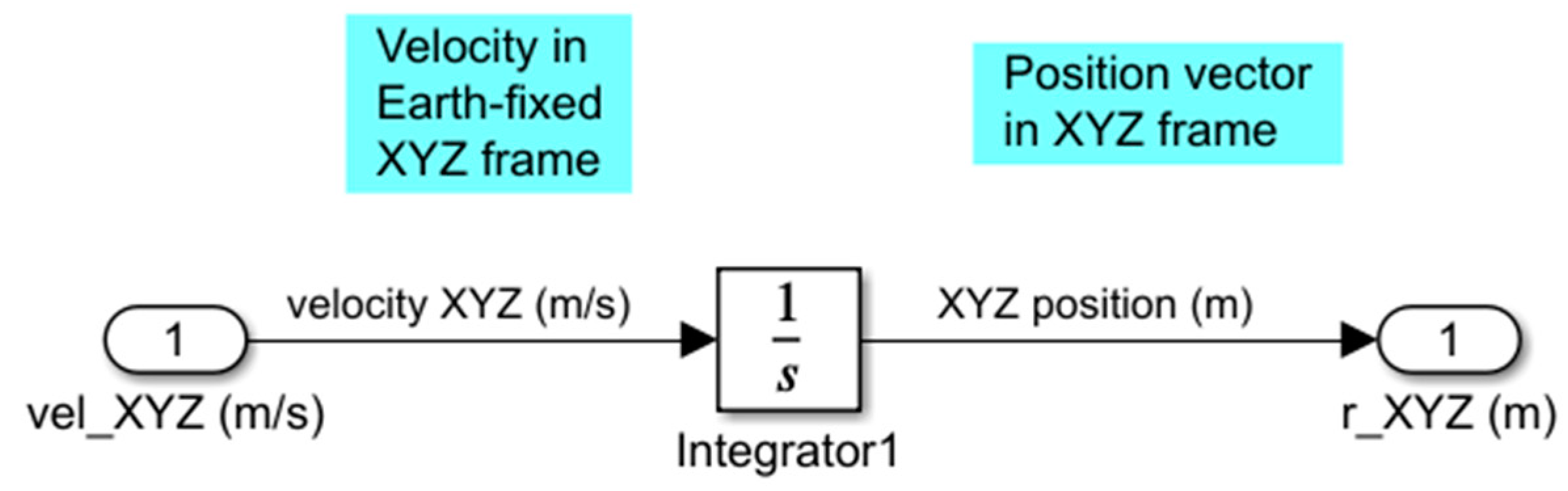
4.2.1. Standard Method for Computing Vehicle Position without Wind

Computing position in simulation is typically the last step after modeling vehicle velocity. Newton–Euler dynamic models typically sum forces and moments in the body-fixed frame to achieve accelerations, and then, velocities in the body-fixed frame. Similarly, for kinematic models, vehicle motion is often specified in the body-fixed frame. So, for both dynamic and kinematic models, the last steps for computing position are:

• Transform the body-fixed velocity, ${\overrightarrow{v}}_g^{xyz}$, to velocity in the inertial or Earth-fixed frame, ${\overrightarrow{v}}_g^{XYZ}$.
• Integrate the Earth-fixed velocity, ${\overrightarrow{v}}_g^{XYZ}$, to achieve position in the Earth-fixed or NED frame:

  $${\overrightarrow{r}}_g^{XYZ}=\int {\overrightarrow{v}}_g^{XYZ}·dt$$

  (20)

It is worth noting here that integrating body-fixed velocity will not generate meaningful results because of the rotating $xyz$ frame. The last step for computing position is illustrated in the Simulink code diagram below (Figure 6). The result is a position vector, ${\overrightarrow{r}}_g^{XYZ}$, in the inertial $\mathrm{X}\mathrm{Y}\mathrm{Z}$ frame.

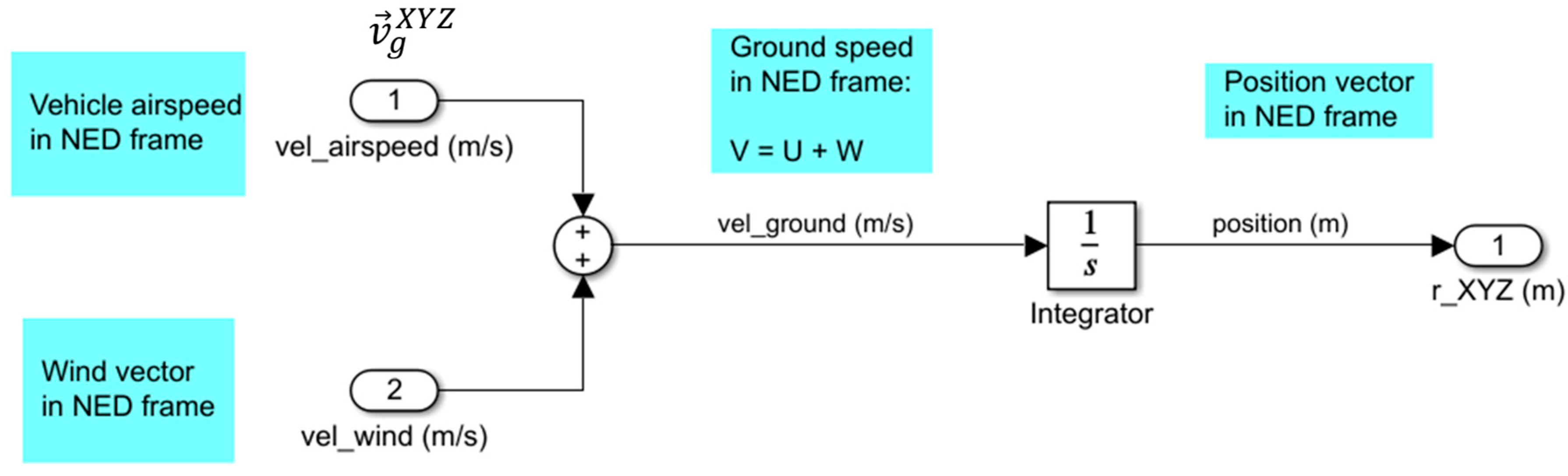
4.2.2. Modeling Vehicle Position with Influence from Wind

To construct a wind triangle, the vehicle velocity in Earth-fixed coordinates, ${\overrightarrow{v}}_g^{XYZ}$, must be relabeled as the vehicle’s airspeed, $\overrightarrow{U}$, which is in Earth-fixed coordinates (e.g., NED frame). Then, the wind triangle is a simple vector addition of airspeed, $\overrightarrow{U},$ and wind speed, $\overrightarrow{W}$, to create the new ground speed vector, $\overrightarrow{V}$. The modified steps for computing vehicle position with the influence of wind are summarized below:

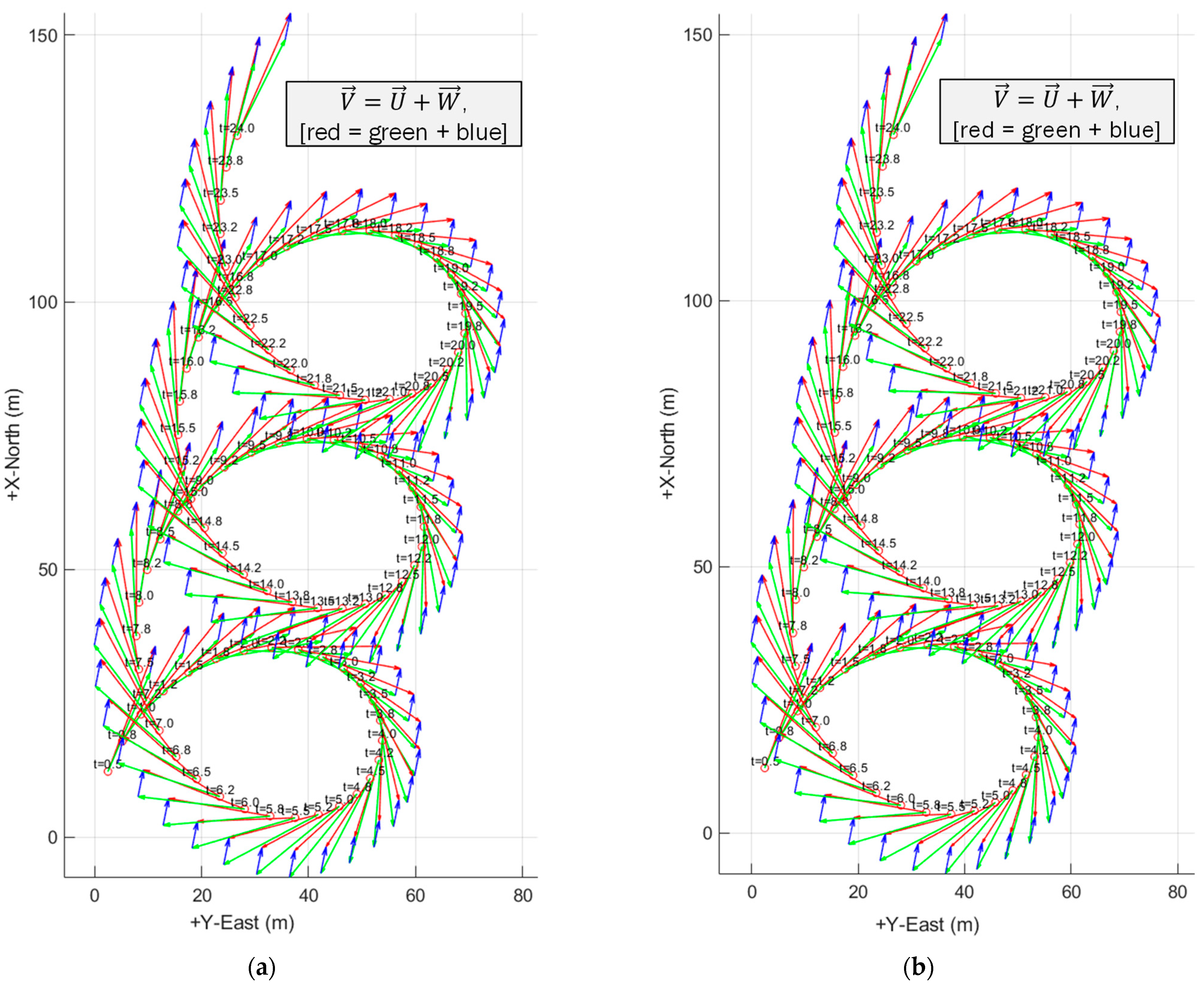
• Assign airspeed to vehicle velocity in the NED frame, or XYZ coordinates: $\overrightarrow{U}={\overrightarrow{v}}_g^{XYZ}$
• Add the wind vector, $\overrightarrow{W}$, to vehicle airspeed, creating the wind triangle relationship: $\overrightarrow{V}=\overrightarrow{U}+\overrightarrow{W}$
• Integrate the new ground speed, $\overrightarrow{V}$, to achieve position in the Earth-fixed NED frame:

  $${\overrightarrow{r}}_g^{XYZ}=\int \overrightarrow{V}·dt$$

To verify this using a simple thought experiment, consider a wind speed vector of zeros. If $\overrightarrow{W}$ = 0, then $\overrightarrow{V}$ = $\overrightarrow{U}$, which simply says that airspeed is groundspeed when there is no wind. This condition is identical to the standard method described in Section 4.2.1. Figure 7 illustrates a Simulink code to compute vehicle position that incorporates the influence of wind. This simulates the wind triangle with a steered vehicle influenced by the wind.

The resulting idealized $\overrightarrow{U}$, $\overrightarrow{V}$, and $\overrightarrow{W}$ vectors are available for careful study and visualization during or after simulation. These relationships are valid for 2D or 3D vectors, and the wind can be modeled simply as a constant or a more complex model like a field that varies with space and time, $\overrightarrow{W}=\overrightarrow{W}(t,X,Y,Z)$.

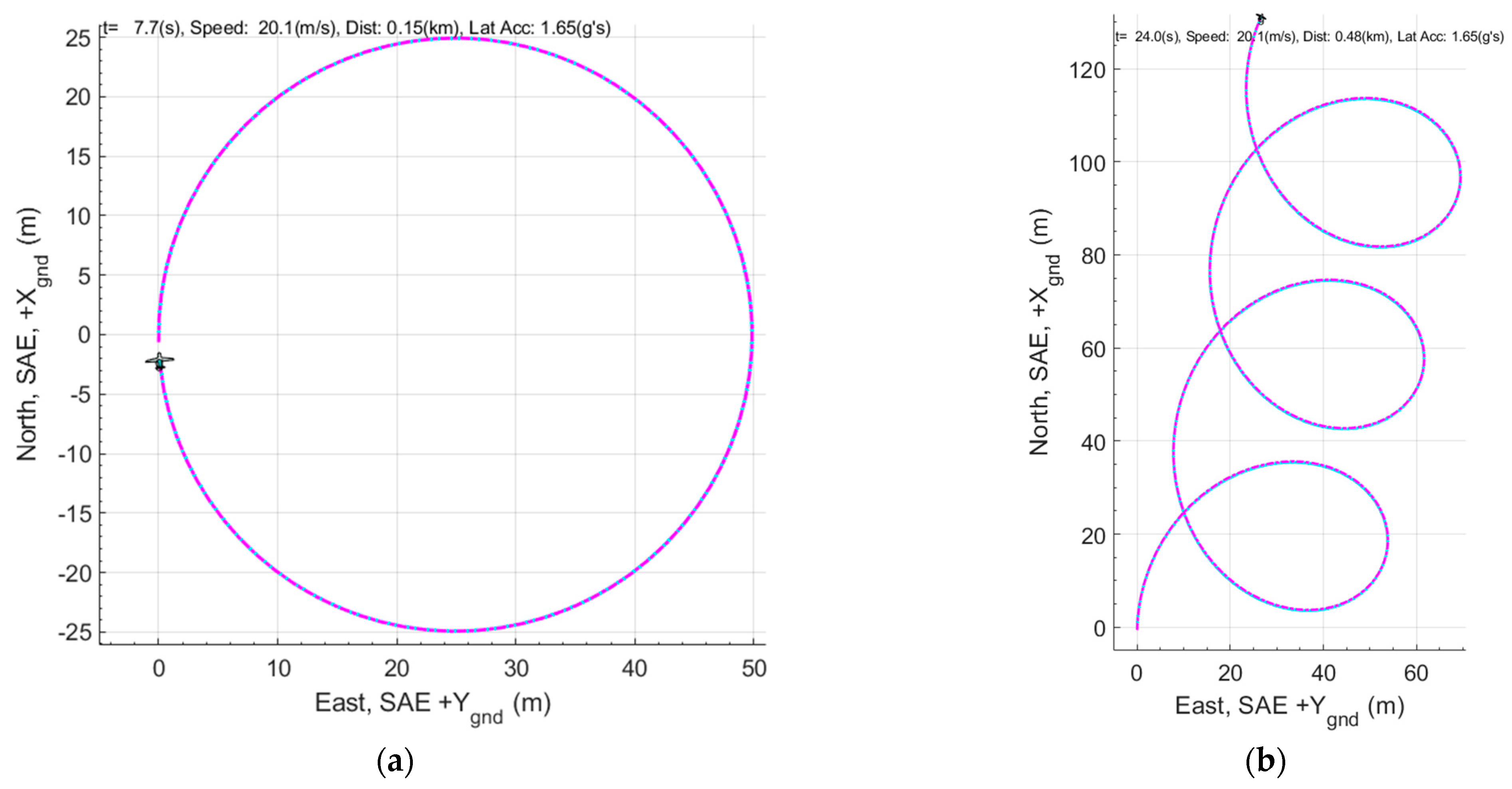
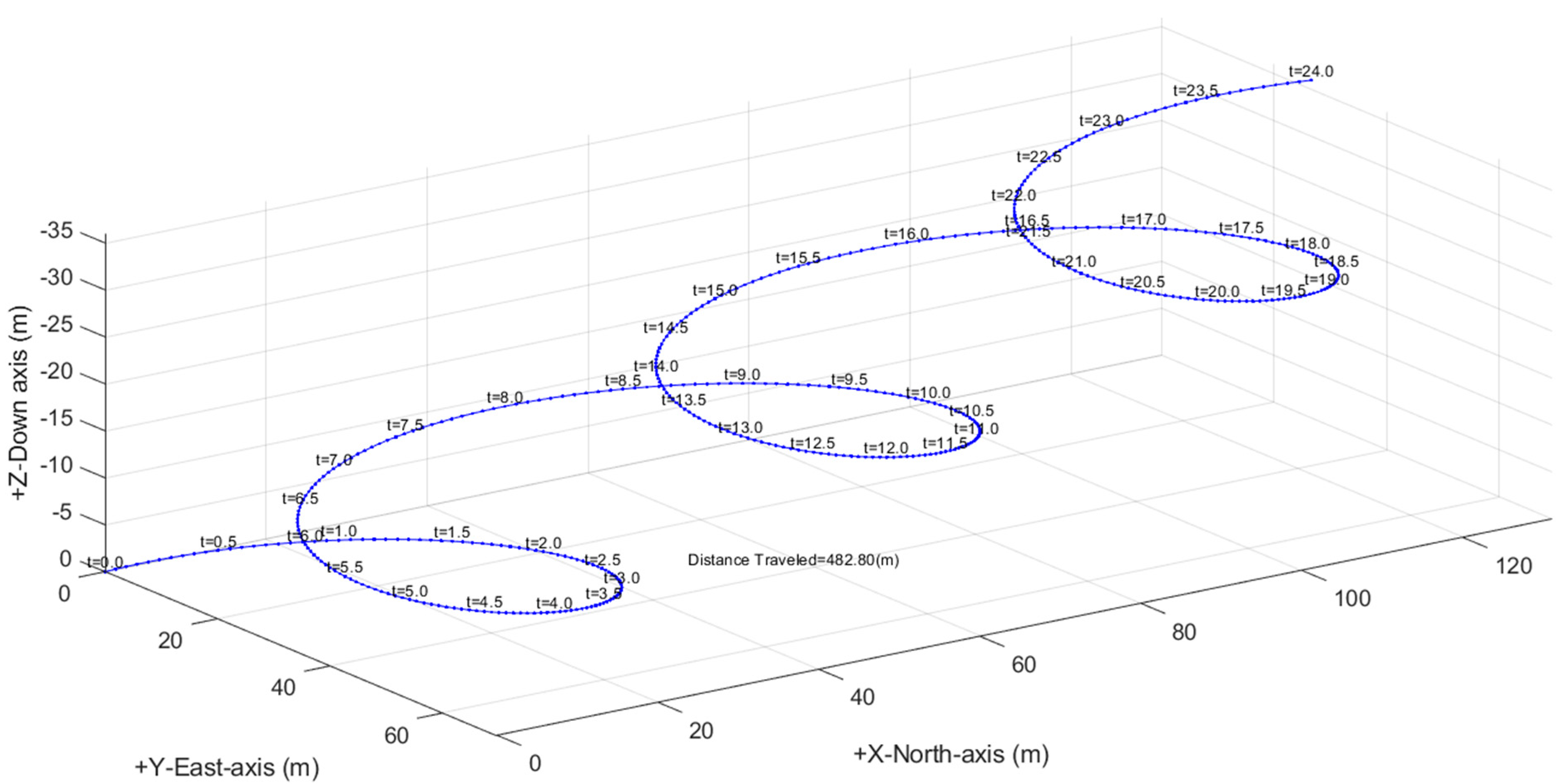
4.2.3. Simulation for Turning Motion with and without Wind

To illustrate this wind estimation method presented in Section 3, the Dubins Aircraft kinematic model, plus the wind model described in Section 4.2.2, and vehicle parameters for a medium-sized fixed-wing aircraft were simulated with a constant turning radius of 25 m.

The simulation provides an excellent environment in which to test the wind estimation algorithms under different wind conditions and verify both their viability and limitations. Figure 8a illustrates the nominal flight path while turning with no wind. A constant radius is expected and shown. Figure 8b illustrates the same steering inputs with wind with $\overrightarrow{W}=\left[51\right]$ (m/s). The expected spiral pattern emerges with an average drift slope of 5:1 in the $NED$ coordinates.

Both of these traces are corkscrew-style traces because a fairly aggressive climb rate of $u_z$ = 300 ft/min (1.5 m/s) is included. Figure 9 shows a 3D perspective of the same simulation as in Figure 8b.

The vehicle and simulation parameters are listed in

Table 1. Fixed-wing simulation parameters.

Parameters	Value
Glide path angle, $\gamma$	4.3°
Wingspan	94 in (2.4 m)
Length	50 in (1.3 m)
Cruise velocity	45 mph (21 m/s)
Elevation rate, $u_z$	300 ft/min (1.5 m/s)

.

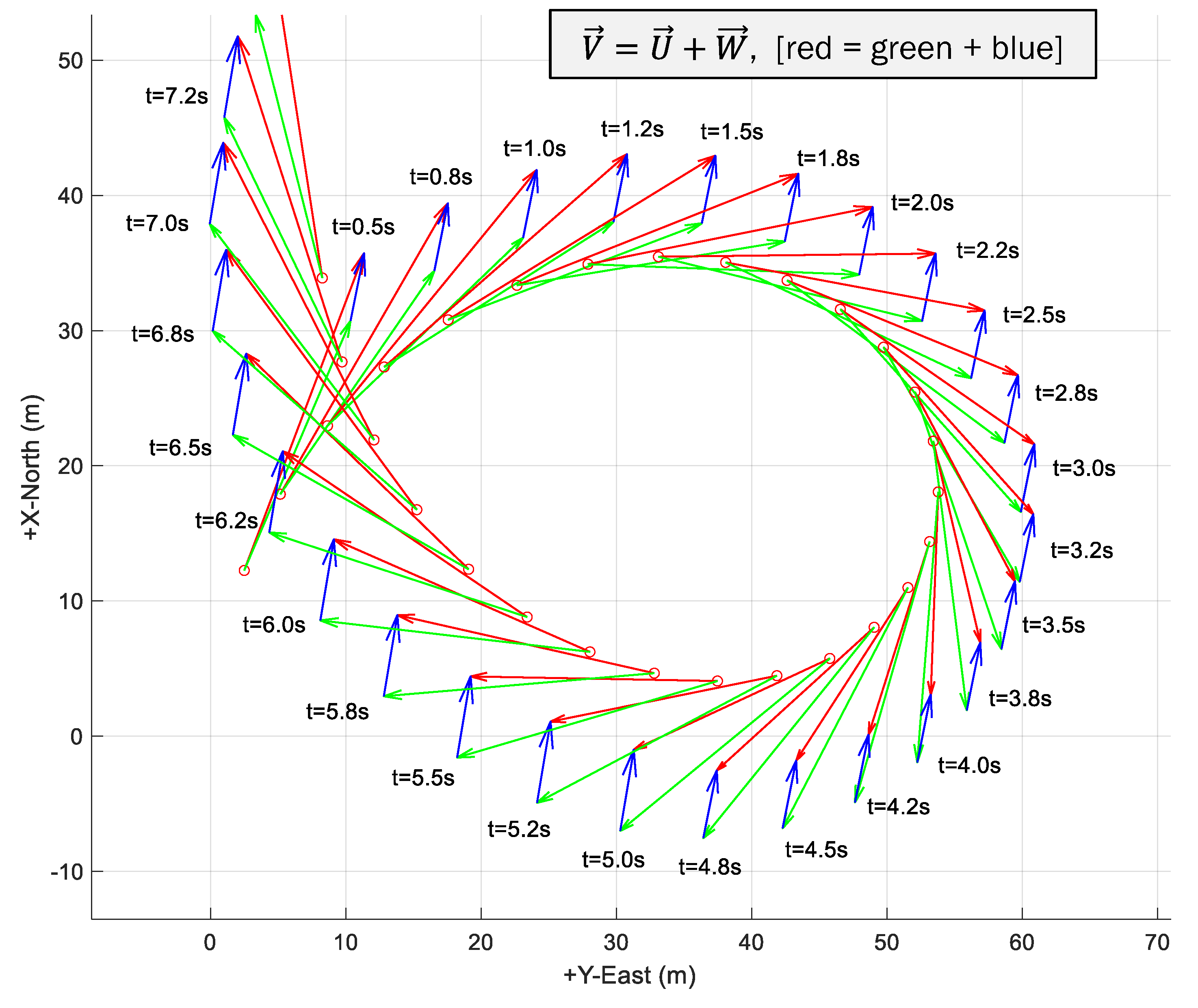
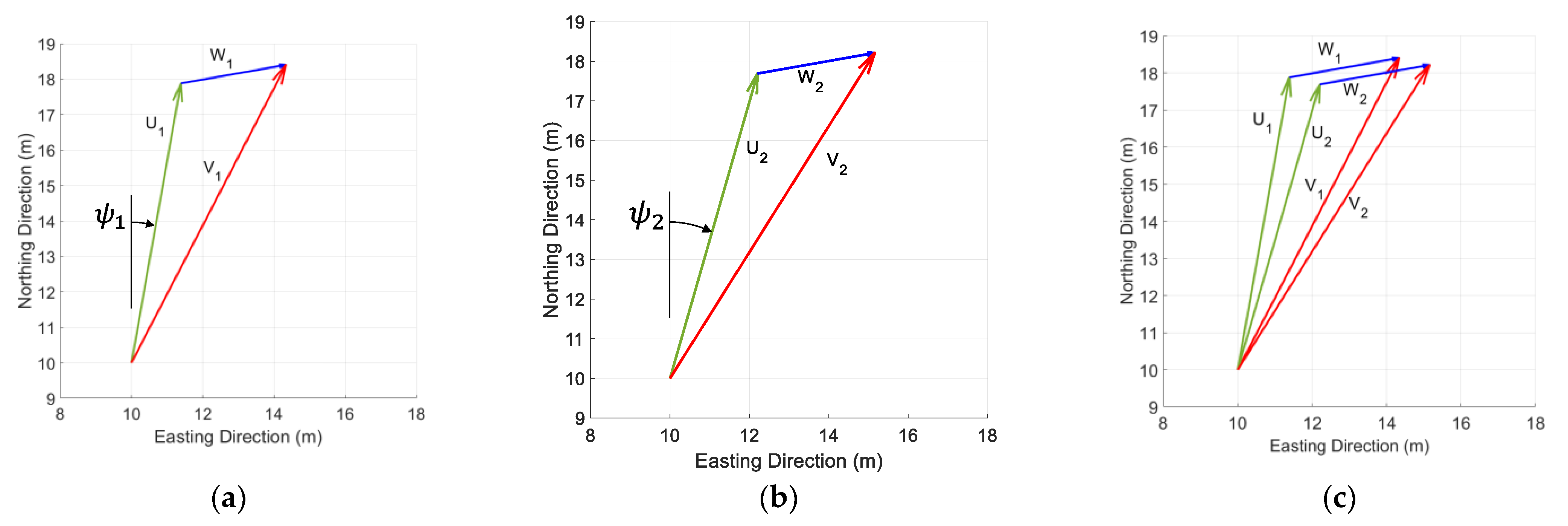
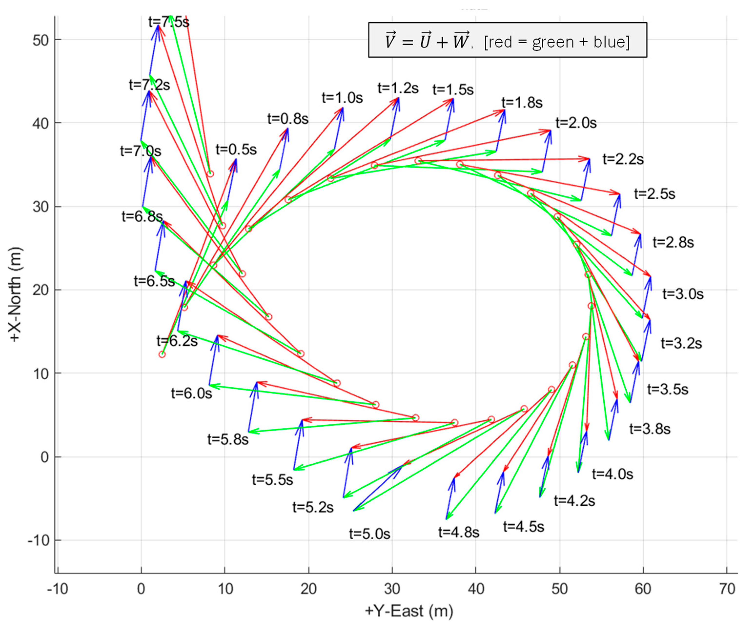
4.2.4. Simulating Wind Triangles

All three idealized wind triangle components are available explicitly in the simulation because ground speed, $\overrightarrow{V}$, is created by adding the vehicle velocity vector, $\overrightarrow{U}$, to the wind velocity vector, $\overrightarrow{W}$. Figure 10a shows the simulated, ideally formed wind triangles at multiple points along the same route from Figure 8b. The Wind-Arc method is also computed using Equations (12)–(16) and shown in Figure 10b. The estimated method’s results are indistinguishable from the idealized $\overrightarrow{U}$, $\overrightarrow{V}$, and $\overrightarrow{W}$ vectors directly from simulation. This shows that the method works as expected under ideal simulated conditions when a constant airspeed and wind assumptions (5) and (6) are met.

The Wind-Arc method is driven by state-based changes in vehicle heading, $\psi$. This is implemented using a capture-and-hold function. When the current heading change from the previously captured heading exceeds a threshold, $\left|\Delta \psi \right|>{\Delta \psi }_{thresh}$, then the second sensor snapshot is captured, triggering the airspeed and wind vector estimates. The only two (simulated) sensors needed to estimate wind triangles in Figure 10 are vehicle heading, $\psi$, and ground speed, $\overrightarrow{V}$, measurable with a compass and GPS.

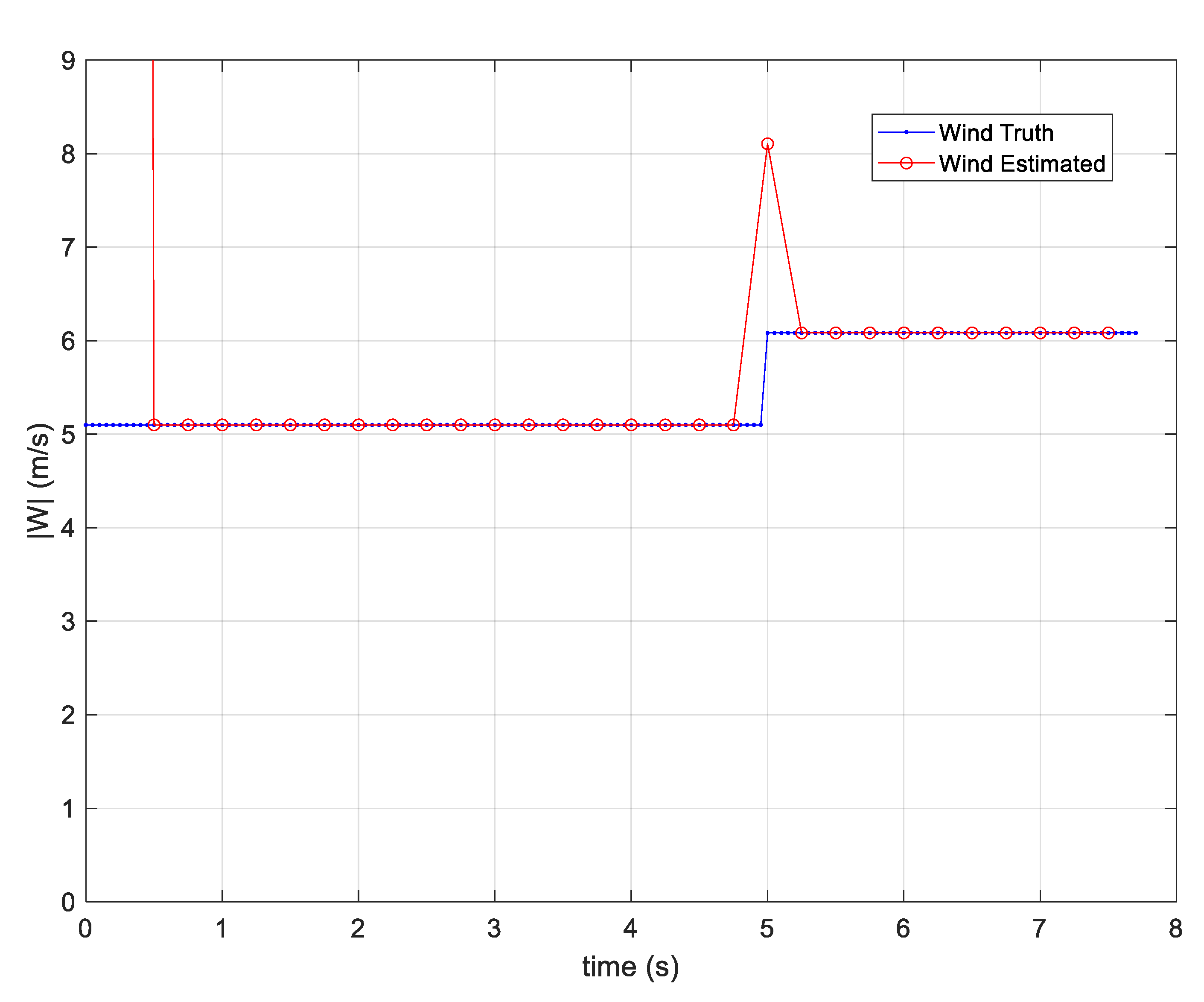
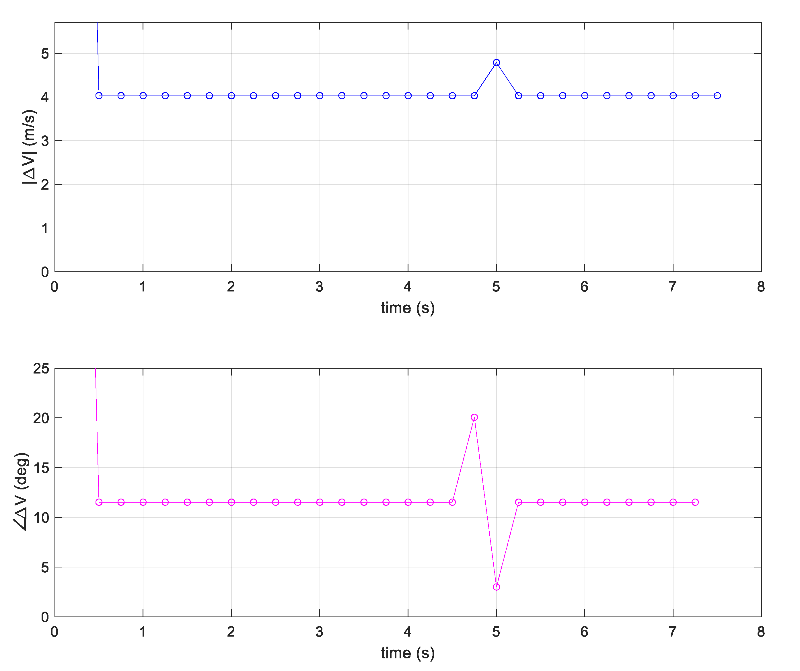
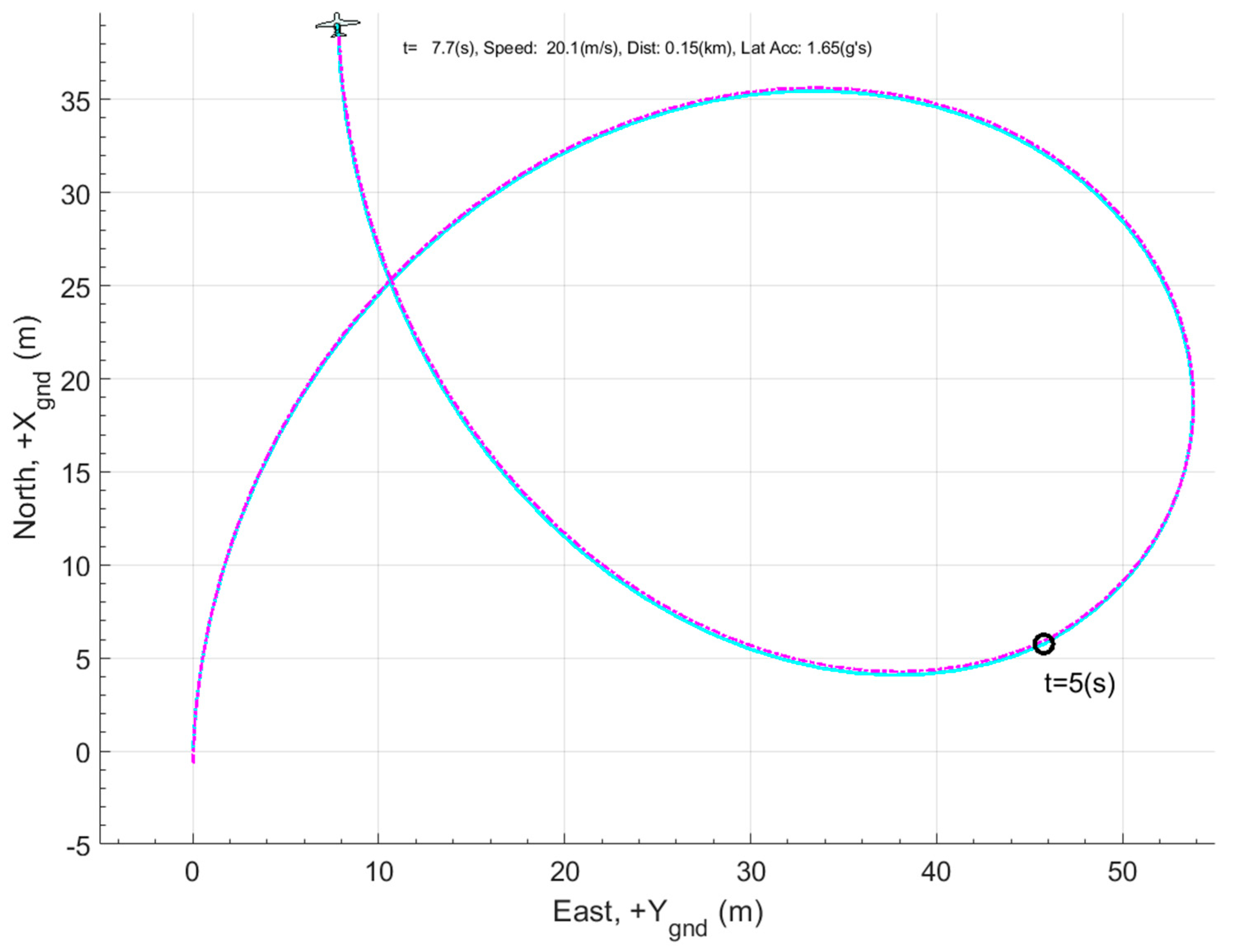
4.3. Simulation Experiment 1: Wind Vector Step Input at t = 5 s

Figure 10 in the previous section shows the sensorless method works under idealized steady wind conditions. During real flights, unknown wind variation will occur. The simulation can provide valuable clues to the method’s capabilities and limitations under changing wind conditions. The next sequence of figures illustrates the same simulated trajectory as above, and a similar wind vector of $\overrightarrow{W}=\left[51\right]$ (m/s). However, a step input of 1 m/s is prescribed at t = 5 s, causing the wind vector to become $\overrightarrow{W}=\left[61\right]$ (m/s). Figure 11 illustrates the trajectory for 7.7 simulated seconds at a nominal cruising speed of 45 mph (22.1 m/s).

Figure 12 compares both the simulated (idealized) and estimated wind vector magnitudes. The two are identical when the constant wind assumption is met, but it is clear that the step input at t = 5 s causes a substantial magnitude error. Also, notice that the estimated wind vector has a one-step convergence period at t = 0 before the well-defined 1–2 point-pairs. Figure 12 shows Wind-Arc estimates occurring uniformly every 0.25 simulated seconds, which represents 4 Hz. Note that this is a state-based trigger resulting from yaw angle changes and not explicitly a function of time.

Figure 13 illustrates the idealized wind triangles directly available in the simulation for the same flight. Notice the idealized wind vector at t = 5.0 s. It is properly formed and oriented and almost imperceptibly changes from $\overrightarrow{W}=\left[51\right]$(m/s) to $\overrightarrow{W}=\left[61\right]$ (m/s) at t = 5 s.

Next, Figure 14 illustrates the method’s estimated wind triangles for the same maneuver and step input at t = 5 s. Notice the malformed wind triangle at the 1 m/s step change from $\overrightarrow{W}=\left[51\right]$ (m/s) to $\overrightarrow{W}=\left[61\right]$ (m/s).

The poor estimate at t = 5 s results from unmet constant wind and airspeed assumptions between successive measurement snapshots. The ground speed vector (red) is different, but almost imperceptibly so, when the step input occurs at t = 5 s. The (green) airspeed vector, $\overrightarrow{U}$, is visibly larger in magnitude and has a larger orientation change than either airspeed vector before or after the step input.

Wind Triangle Error Analysis

Recall that the airspeed vector is estimated using Equation (13): ${\overrightarrow{U}}_1=N^{-1}·\left[{\overrightarrow{V}}_2-{\overrightarrow{V}}_1\right]$. To understand which term causes the malformed triangle at the step-change in wind, consider the two terms: $N^{-1}$ and $\overrightarrow{\Delta V}$. The matrix $N$, and its inverse will be well behaved because the heading angle change, $\Delta \psi$, is a predictable value based on the vehicle’s captured yaw angles, ${\psi }_1$ and ${\psi }_2$. Matrix $N$ and its inverse will have a good condition number and be nearly identical before, during, and after the step input. The unexpected change occurs in the groundspeed term, $\overrightarrow{\Delta V}={\overrightarrow{V}}_2-{\overrightarrow{V}}_1$. This vector, $\overrightarrow{\Delta V}$, represents the tip of one (red) ground speed vector, ${\overrightarrow{V}}_1$, to the tip of the next subsequent vector ${\overrightarrow{V}}_2$. Figure 15 shows both the magnitude, $\left|\overrightarrow{\Delta V}\right|$, and sequential heading angle changes, $\mathrm{\angle }\overrightarrow{\Delta V}$. The figure shows a noticeable magnitude change and also a noticeable orientation change at the t = 5 s wind step input. The angle change is initially larger, and then, smaller, before and after the wind step change. This signature, combined with the magnitude change, is an indicator of the method’s potential low-quality estimate when constant wind assumptions are not met.

This section has demonstrated that the Wind-Arc method provides perfect performance during idealized, simulated conditions. The method captures successive heading angle and velocity vectors as the only sensed values necessary to estimate wind direction and magnitude. It also shows results from a 1 m/s step input in the wind vector and presents results when the constant wind assumptions are not met.

5. Results from Real Flight Tests

This section demonstrates the new method’s validity using experimental data from two separate vehicles. Real flight data were collected from instrumented aircraft to compare the Wind-Arc method to the flow sensor approach. First, flight test results from a fixed-wing aircraft, and then, flight test results from a multi-rotor vehicle are shown. Both aircraft are instrumented in order to compare the Wind-Arc method to the Direct Flow Measurement method.

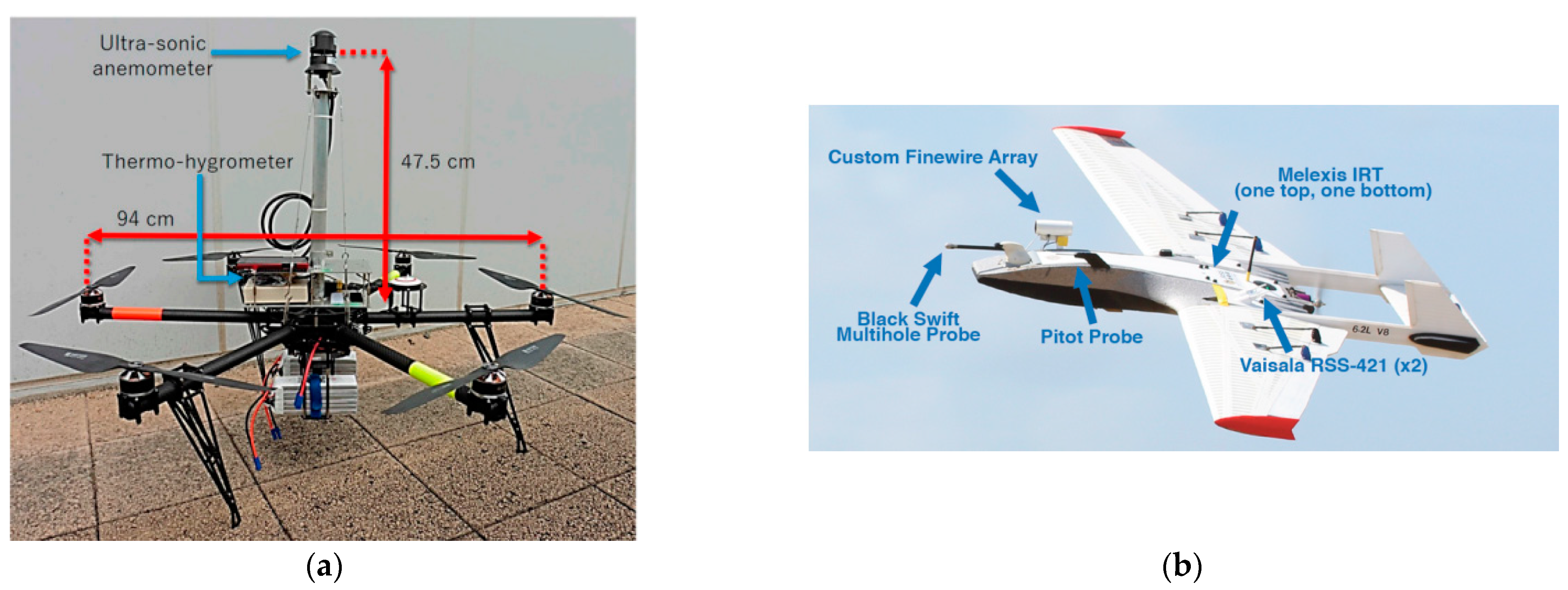
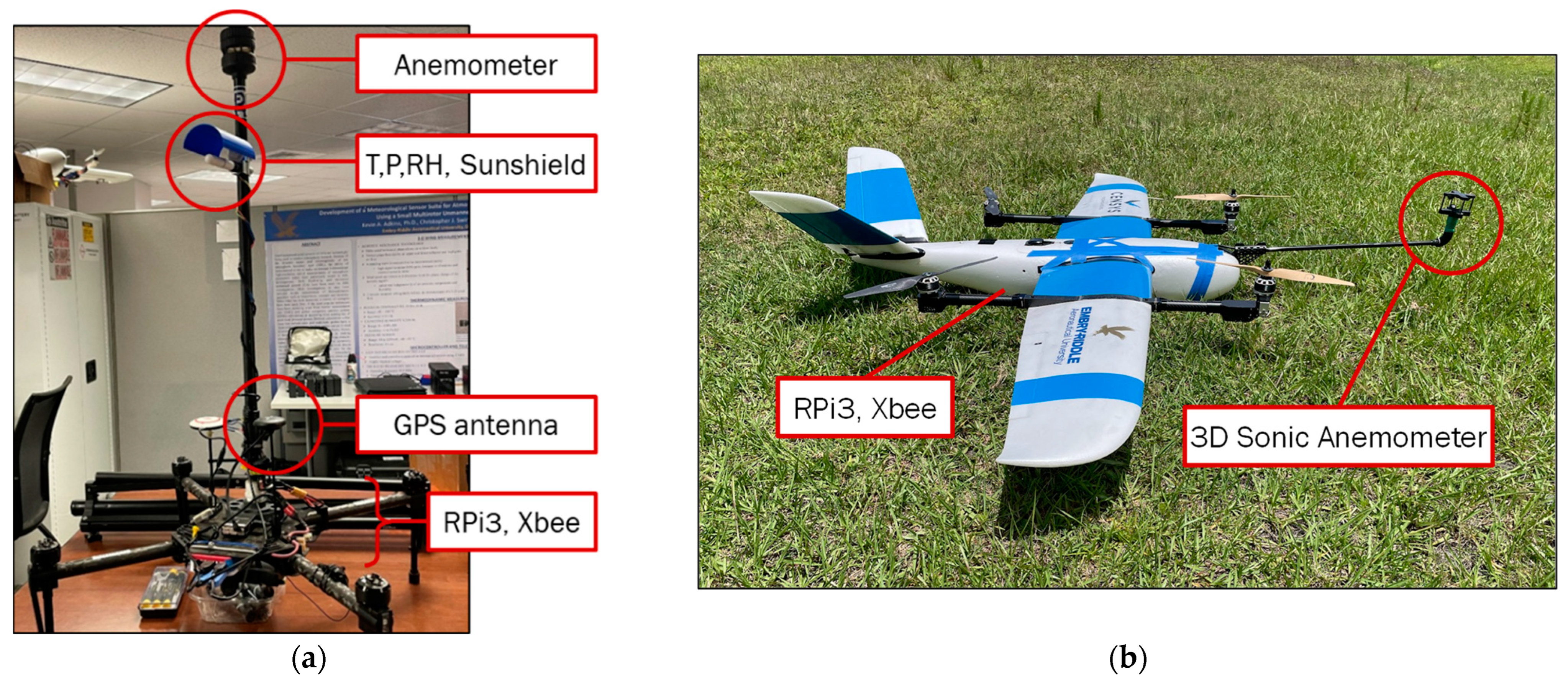
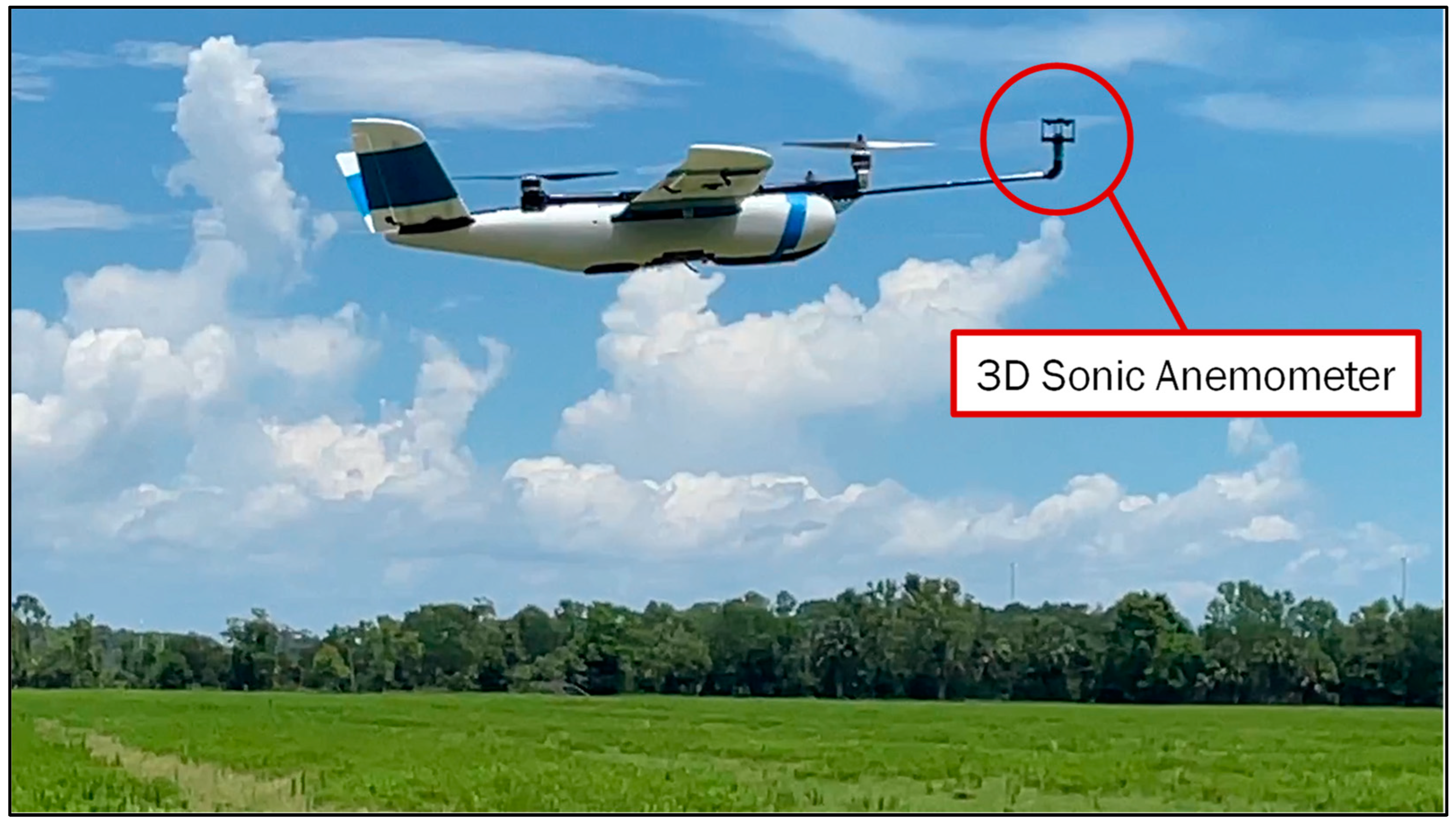
5.1. Experimental Vehicles and Instrumentation

The multi-rotor UA shown in Figure 16a is a DJI Matrice 100 instrumented with an FT-205 AcuRes Anemometer that logs a 2D airspeed measurement at 10 Hz. The fixed-wing UA shown in Figure 16b is a VTOL Censys Sentaero with a TriSonica Mini ToF Anemometer that logs a 3D airspeed measurement at 10 Hz. Both data acquisition systems are powered and controlled by a Raspberry Pi 3 with an additional Pixhawk v4 Mini specifically installed to provide the vehicle velocities and orientations. This flight controller is an additional payload that is not used to control the aircraft and is used solely for data collection purposes. In both vehicles, the anemometer estimates airspeed in the body-fixed frame and vehicle speed using GPS velocity and Course Over Ground (COG). Post-processing is performed to transform the body-fixed airspeed vector into the $NED$ frame, $\overrightarrow{U}$. Then, airspeed is subtracted from ground speed in Equation (1) to estimate wind using $\overrightarrow{W}=\overrightarrow{V}-\overrightarrow{U}$.

5.2. Flight Test #1 with Fixed-Wing Aircraft and Trisonica 3D Sonic Anemometer

This section presents the experimental results from a fixed-wing aircraft flying waypoint-based missions at an airfield near Daytona Beach, Florida. The aircraft flown was a Sentaero Vertical Take-off and Landing (VTOL) aircraft manufactured by Censys Technologies Inc. in Daytona Beach FL, USA [64] with a cruise speed of 45 mph (Figure 17).

Figure 18 is a Google Earth view of the total VTOL flight pattern that spanned the entire airfield. Take-off and landing are shown on the far left, and the two separate loiter circles include multiple rotations with a constant radius at two different elevations.

The vehicle missions were designed using Mission Planner v1.3 software, and then, executed using the on-board Pixhawk4 flight controller to fly the aircraft to each waypoint in automatic navigation mode. The standard take-off and landing maneuvers, plus the loiter circles, were all typical for VTOL flight. But the straight sections had waypoints specifically chosen with alternating lateral offsets to induce both left and right turning for the Wind-Arc method. Figure 19 displays specific segments of the broader flight path differentiated with color. These segments were created by selecting points of interest, and then, using a simple algorithm to segment the path into smaller portions for discussion and investigation. The lateral offsets in segments 4, 6, and 7 were designed as zig-zags specifically to exceed the yaw angle change that triggers the Wind-Arc method.

Figure 20 reveals the zig-zag patterns in segments 4, 6, and 7 did, indeed, provide enough yaw angle change to achieve good wind triangles, and thus, good wind estimates. The loiter circles provide regular updates while circling. The prevailing winds were west–north-west at 10–15 mph just prior to a summer rainstorm passing through, so some variation in wind speed and direction is expected.

Figure 21 shows a closer view of the wind triangles in segments 4, 5, and 6 and reveals how important the yaw angle changes are during the zig-zag waypoint patterns. The method’s current formulation requires successive rotations in Equation (2) to exceed a threshold, ${\Delta \psi }_{thresh}$. The results are shown using ${\Delta \psi }_{thresh}$ = 10 deg. When this state-based threshold is exceeded, there are wind estimates, and vice versa. Notice that the method works well when traveling downwind, cross-wind, and upwind. Careful inspection of the red arrows (GPS velocities) reveals larger ground speeds when traveling downwind compared to upwind. Airspeed is approximately constant because the vehicle speed command was approximately constant during automatic waypoint flight. This means the green arrows (airspeed) are approximately the same length throughout but the red arrows (GPS ground speed) change with the direction of travel.

Figure 22 shows a closer view of two loiter circles. Again, careful inspection of the GPS velocities (red arrows) illustrates a larger ground speed vector when flying downwind. Only two loiter circles are shown for visual clarity.

Figure 23 shows a comparison between the sonic anemometer’s measured airspeed during all segments, including the VTOL vertical transitions to and from forward flight. The anemometer’s measured airspeed (blue) is mostly steady during forward flight. The Wind-Arc method shows very good agreement with the measured anemometer data, with the average (maroon) showing a small positive bias relative to the anemometer. Wind-Arc updates occur, on average, every 0.5 (s), which represents 2 Hz. Anemometer updates occur at 10 Hz.

Figure 24 shows the wind speed estimates from the sonic anemometer after subtracting vehicle velocity and compares this to the Wind-Arc method.

Wind is a difficult quantity to measure, so error is a difficult quantity to estimate. The anemometer method provides the most accurate estimate, but philosophically and practically, there are still errors present. Therefore, what is presented here is the differences between the two estimates. Figure 25 shows the difference between airspeed and wind speed for both the anemometer-based method and the Wind-Arc method.

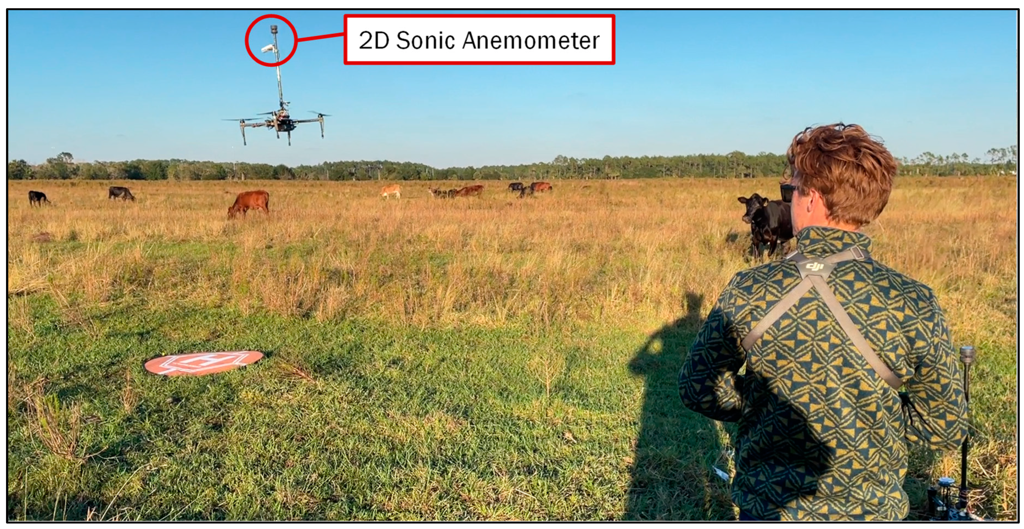
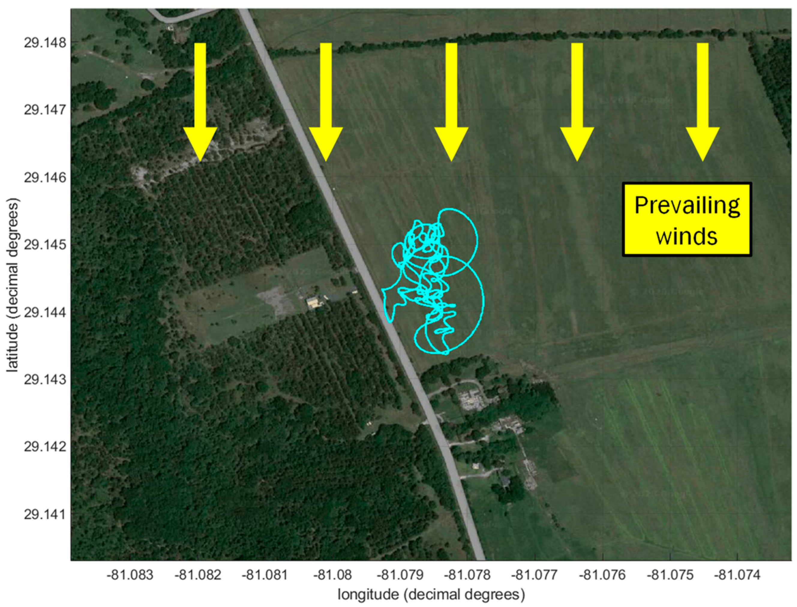
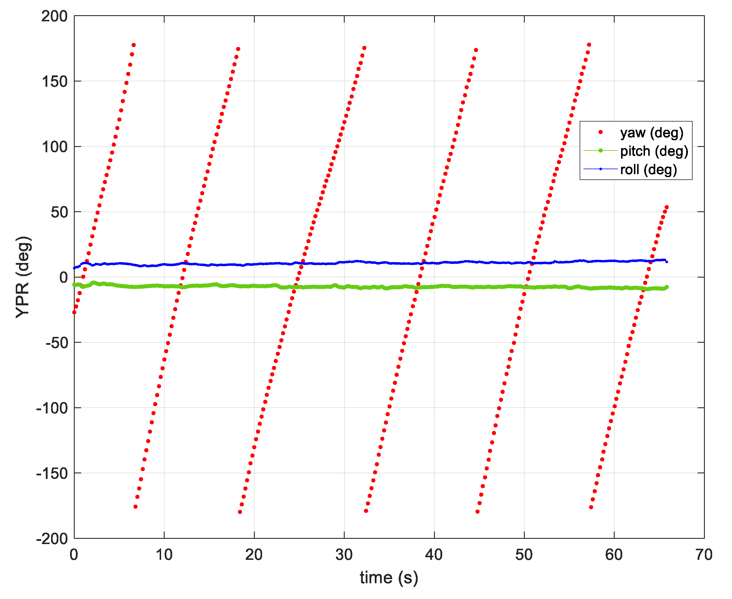
5.3. Flight Test #2 with Multi-Rotor Aircraft and FT205 2D Sonic Anemometer

This section presents wind estimation using a multi-rotor vehicle flown in such a way as to collect successive positions and orientations suitable for the Wind-Arc method. The Wind-Arc method estimates wind using successive wind triangles after a small rotation, which is typical of fixed-wing flight. But this is also quite easily achievable using a multi-rotor aircraft. The Wind-Arc method may be particularly appealing with multi-rotor operations because of their omnidirectional motion. This capability, plus the difficulty of avoiding rotor wash, make it difficult to incorporate a directional sensor, like a Pitot tube or MHPP, on a multi-rotor UA.

The pilot flew the multi-rotor in a manner where yaw motion was coordinated with forward motion, similar to a fixed-wing aircraft. Achieving flight with maximum translational influence from the wind was the goal. The impressive piloting skills are shown below, but once the sequence began, complexity and cognitive load were relatively low. The maneuvers were performed using a ‘manual’ flight controller mode, which engaged the flight controller’s orientation stability mode but made no attempt to reject lateral, translational motion from wind. Launching from an open field, the pilot performed several extended manual-mode maneuvers while intentionally allowing the vehicle to drift downwind.

Figure 26 shows the multi-rotor vehicle flying in manual flight mode with a Part 107-qualified pilot. The 2D sonic anemometer is visible on a custom mast designed to avoid sensing rotor-induced air flow. The white solar radiation shield is also visible to ensure the scalar temperature and humidity sensors measure ambient T and RH.

Figure 27 illustrates the open field and approximately 12 min of GPS traces viewed from above. The prevailing winds caused the vehicle to translate downwind while turning with a constant radius.

Post-processing flight data involved segmenting the entire flight into sub-segments based on location and yaw-rate. One segment within the complete flight record is particularly well suited to illustrating the Wind-Arc estimation method. Figure 28 isolates this sequence of a nearly constant yaw rate resulting in a downwind spiral.

The pilot’s manual inputs would have achieved a mostly constant radius turn for just over a minute if wind speeds were zero. But fairly constant winds from the north caused the southward spiral pattern shown in Figure 28. Yaw, pitch, and roll for the approximately 65 s of data recorded are shown in Figure 29 and illustrate the multi-rotor orientation during five spirals. Figure 29 illustrates excellent piloting skills in manual flight mode that mimic fixed-wing motion with coordinated forward motion and associated yawing motion.

Applying the Wind-Arc algorithm to this flight resulted in the blue wind estimate illustrated in Figure 30.

Figure 30 clearly shows red velocity vectors tangent to the path. These are directly measured using GPS velocity and Course Over Ground. The Wind-Arc method estimates the vehicle airspeed, with the green arrows and blue wind vectors at each estimation location determined by ${\Delta \psi }_{thresh}$. The wind vectors vary, but generally point toward the south with a magnitude that could reasonably represent the prevailing winds experienced that day during testing. The vehicle’s on-board sonic anemometer measured airspeed, which is compared to the estimated airspeed in Figure 31 below. Wind-Arc estimates occur, on average, every 0.2 (s) which represents 5 Hz updates. Again, this is state-based and not time-based, so the Wind-Arc frequency is a function of yaw rate. The anemometer updates also occur at 5 Hz on the quad-rotor, which is slightly different than the sensor in flight test #1.

Wind speed is computed by subtracting (measured) airspeed from vehicle speed, $\overrightarrow{W}=\overrightarrow{V}-\overrightarrow{U}$. The resulting wind speed is compared to the Wind-Arc estimate in Figure 32 below.

Figure 32 shows Wind-Arc results (in blue), which follow the wind speed trend from anemometer-derived results. Again, similar to the previous flight test, wind is a difficult quantity to measure, and both the anemometer-based approach and the Wind-Arc method have errors resulting from the true wind speed. Philosophically, the true wind speed with no error is not available, so what is shown is two wind speed estimates, both of which contain some amount of error. Figure 33 shows the difference between the anemometer-based airspeed and wind speed and the Wind-Arc method.

Both wind estimates rely on GPS velocity and Course Over Ground (COG), but the Wind-Arc method provides a substantially simpler approach to data collection and post-processing. Multi-rotor Flight Test #2 appears to have better quality airspeed and wind estimates compared to the fixed-wing experiment in Flight Test #1. Understanding fundamental reasons for the higher- or lower-quality Wind-Arc estimates will be the aim of future work.

6. Discussion

From the simulation and experimental results, the following points are clear:

• The Wind-Arc method provides perfect performance both analytically and in simulation under constant wind and ideal sensor conditions. The simulation-based experiments validate the approach, underlying theory, assumptions, and performance. Under real flight tests, the method works well with some moments of unexpected magnitude and direction change.
• Anomalies in the Wind-Arc estimates are attributable to the following: (a) unmet airspeed or wind speed assumptions, (b) GPS errors, (c) heading or orientation errors, and (d) data logging delays.
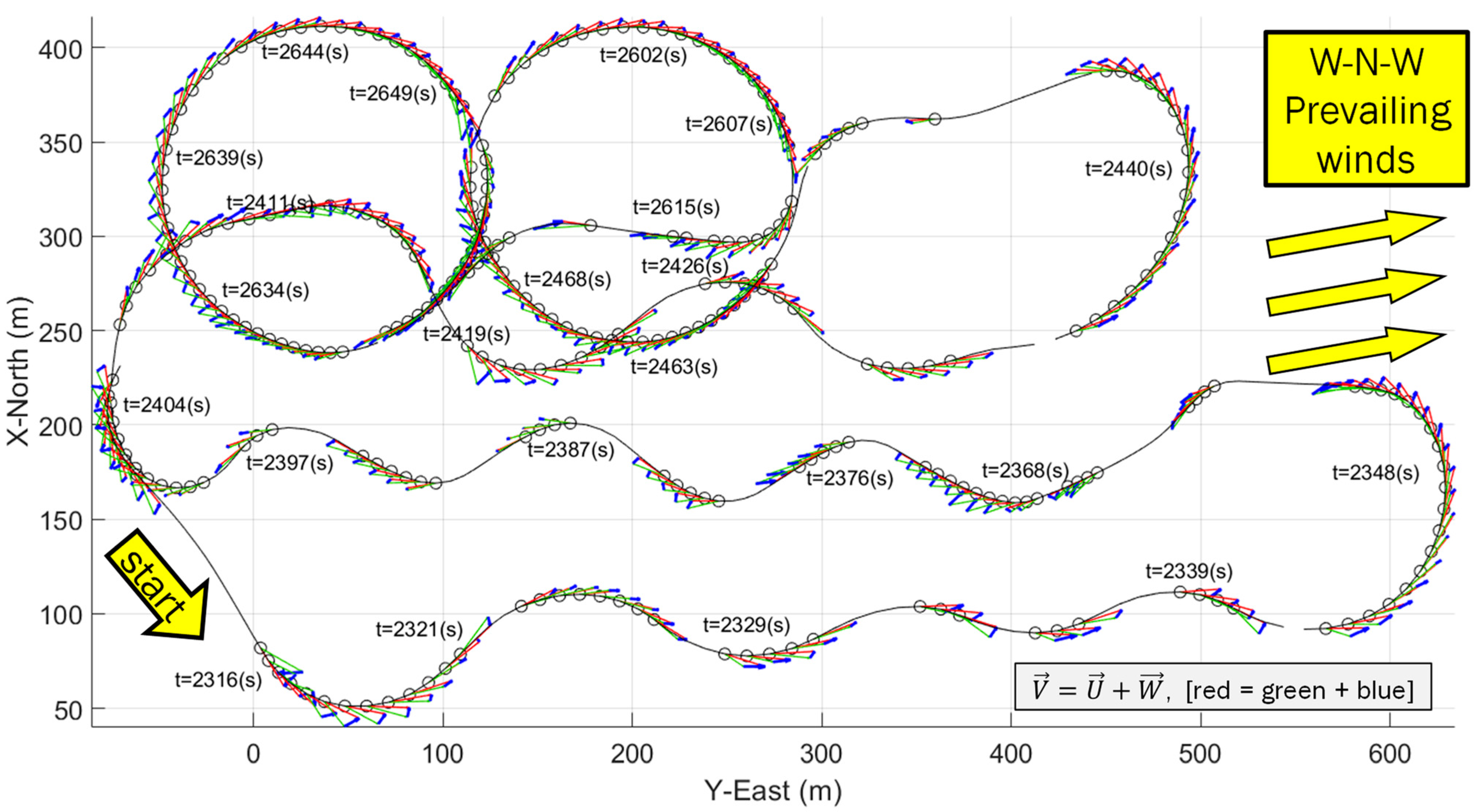
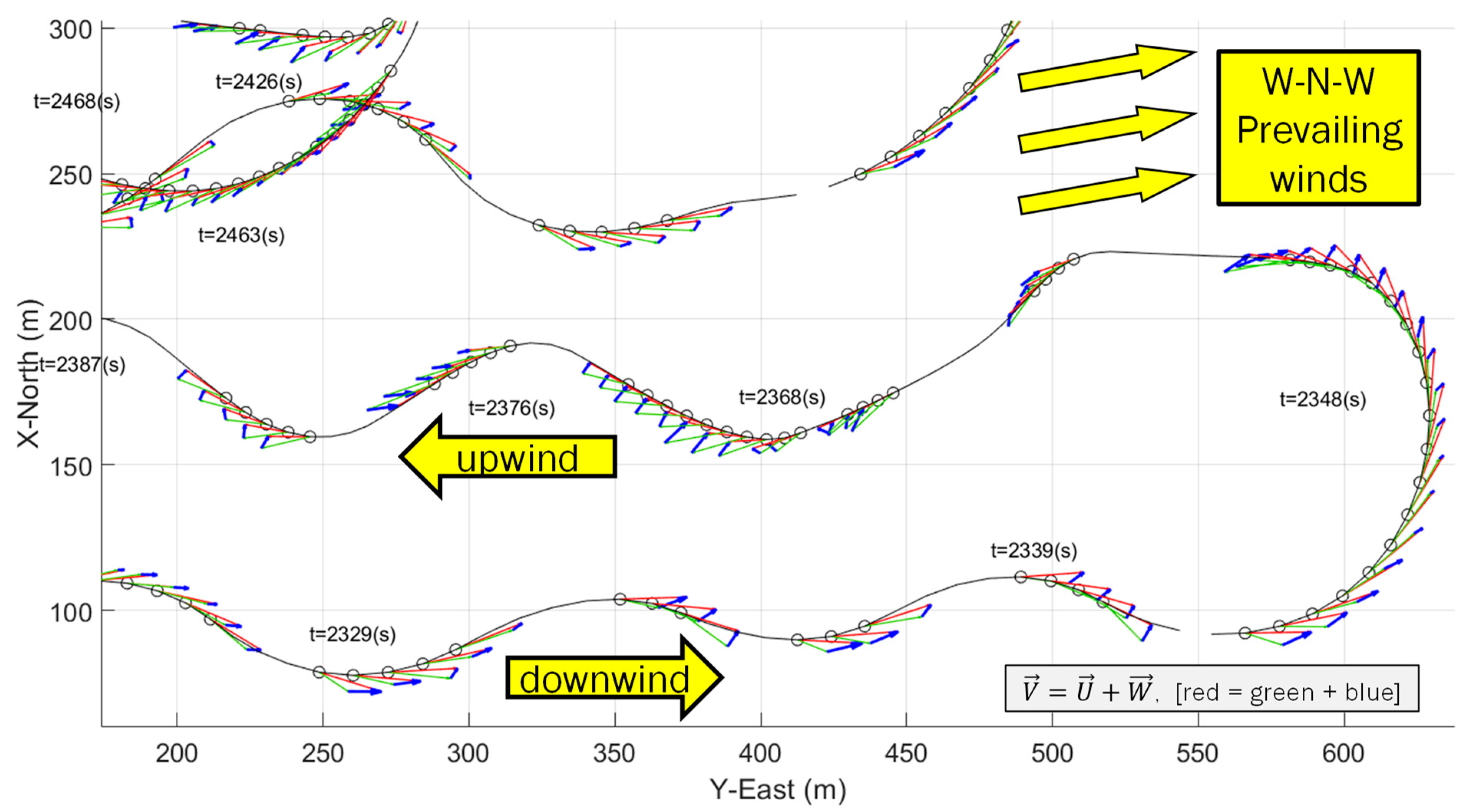
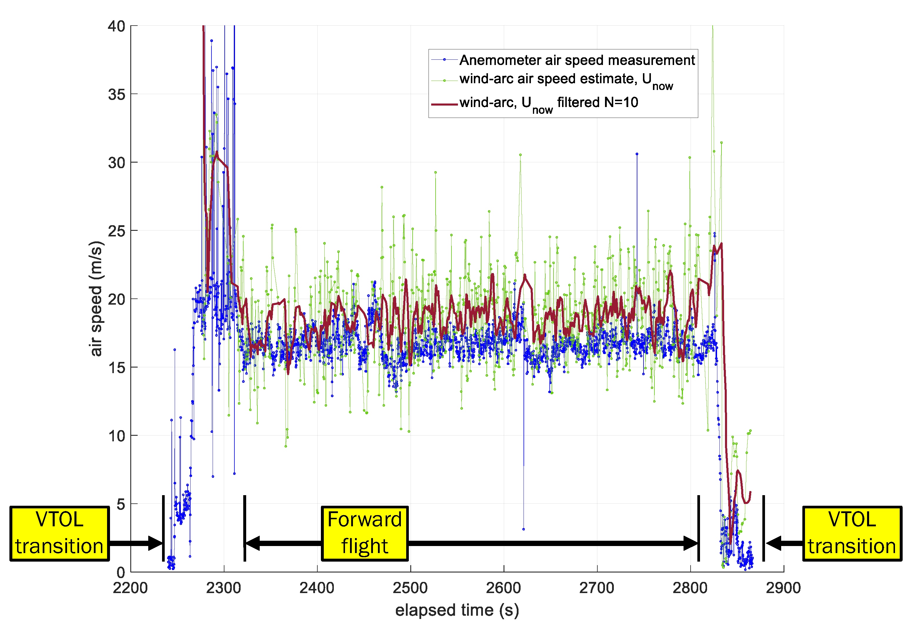
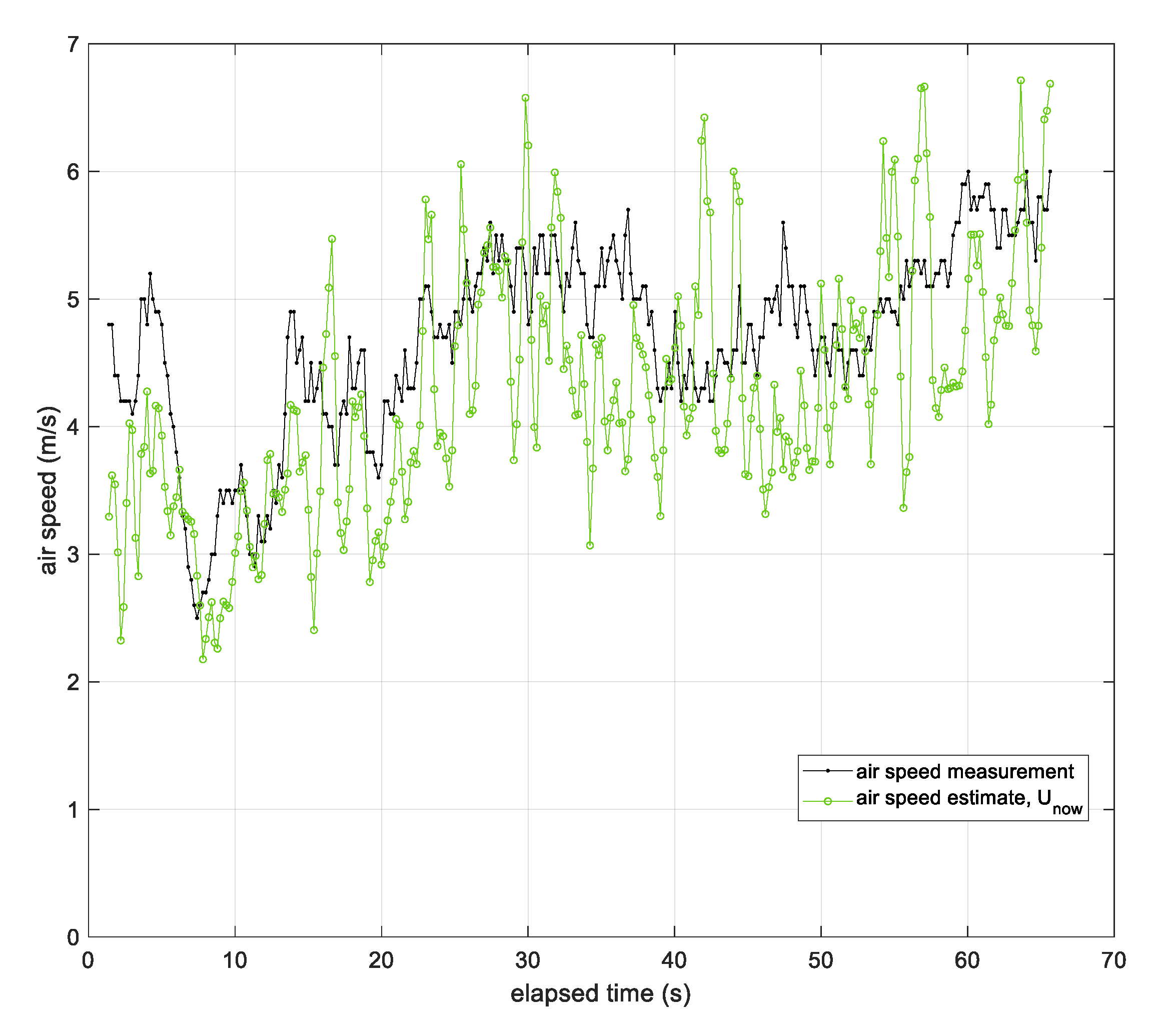
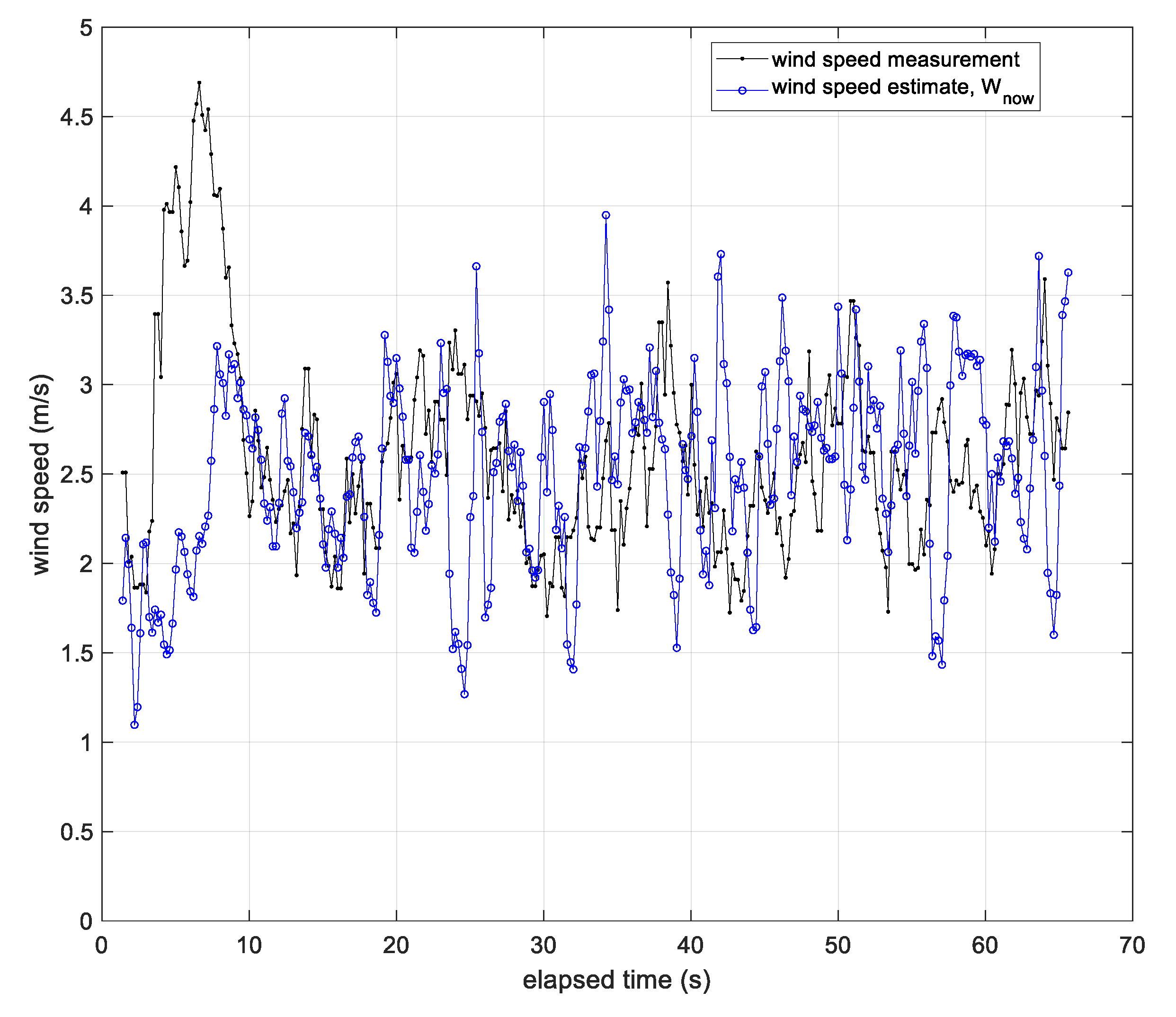
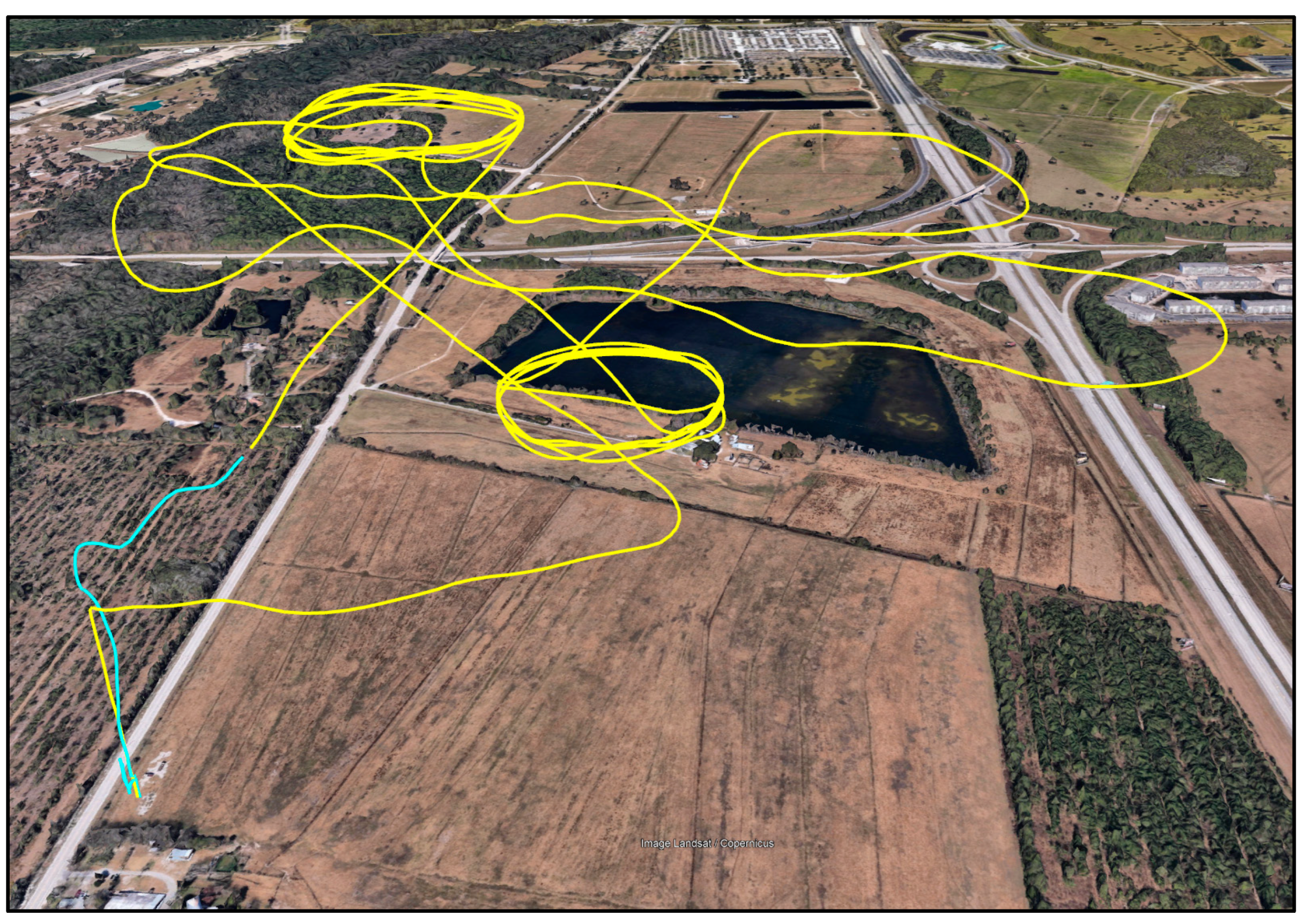
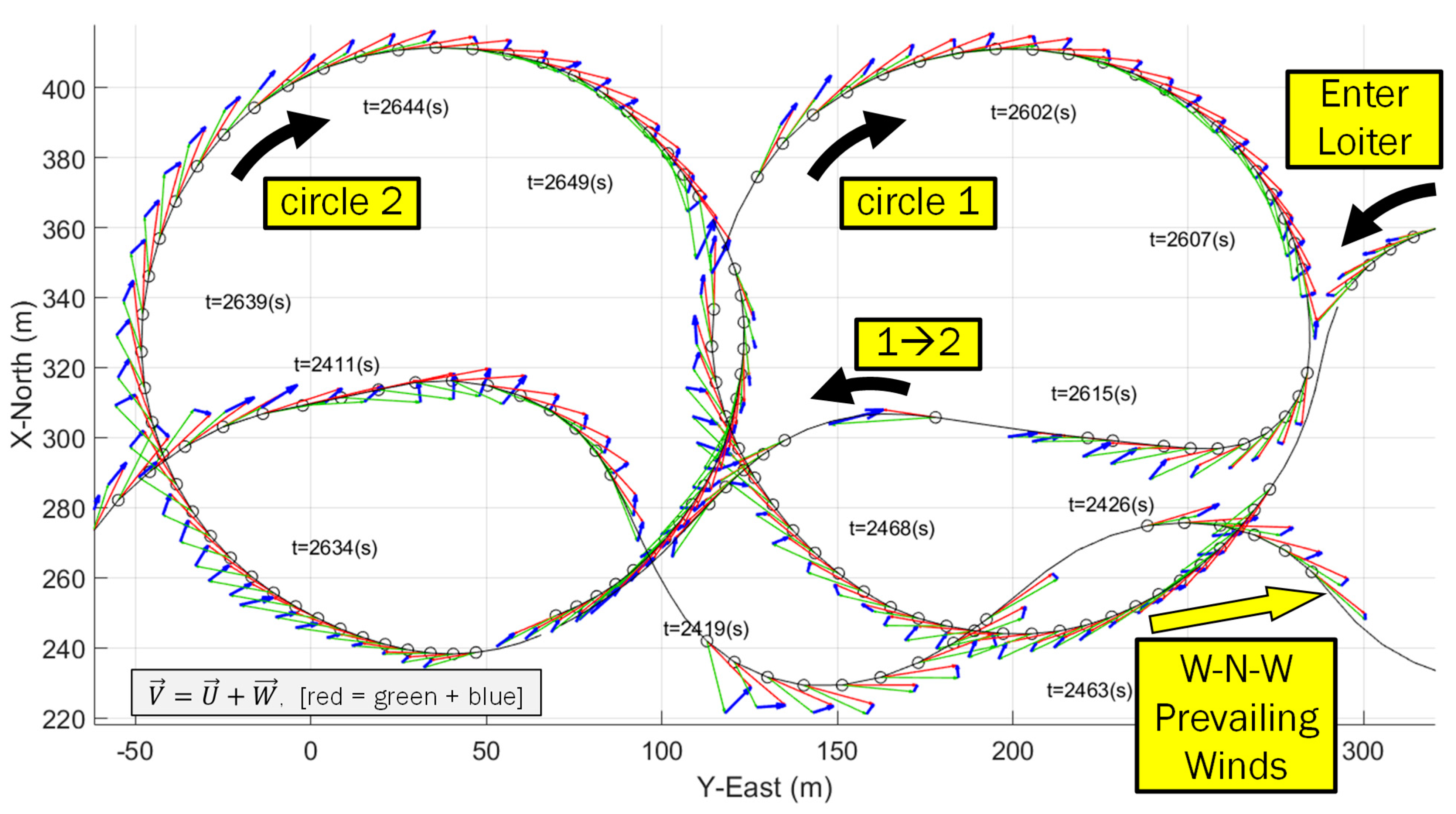
• The anemometer measuring airspeed in both experiments has some variation but is bounded around an average airspeed. This means that airspeed variation was not the dominant source of wind variation. For example, in Figure 23, the anemometer’s airspeed is approximately constant, with the exception of two locations (t = [2450 s, 2625 s]) where the vehicle changed altitude to enter and exit the first loiter circle. This indicates, for this particular example, the vehicle’s forward throttle maintained a nominal airspeed within the surrounding air mass. It also suggests the surrounding air mass moved as a coherent volume such that the entire air mass, with the vehicle, changed ground speed as the wind speed changed regardless of the vehicle’s traveling direction (upwind or downwind).
• One possible source of unexpected anomalous wind estimates is the term $[{\overrightarrow{V}}_2-{\overrightarrow{V}}_1]$ in Equations (14) and (15). GPS velocity is one of the most accurate sources of outdoor horizontal velocity measurements globally [65], so this term is not the most likely source of unexpected errors. But GPS error is still worth exploring using Horizontal and Vertical Dilution of Precision metrics, or HDOP and VDOP, respectively. These HDOP and VDOP values are embedded in GPS messages and can be recorded and studied in future work to determine the error associated with the $[{\overrightarrow{V}}_2-{\overrightarrow{V}}_1]$ term.
• Wind-Arc sample rates are based on state changes in the yaw angle and are not determined strictly by time. The simulation experiments and both flight tests 1 and 2 showed Wind-Arc estimates at 5 Hz, 2 Hz, and 5 Hz, respectively. This means the Wind-Arc method, from these experiments, is best suited for estimating the lowest average wind speed and is not currently a good candidate for turbulent wind measurement.
• Wind shear is defined by a velocity gradient across scales in the tens or hundreds of meters. The Wind-Arc method requires constant wind between two successive snapshots. There is no mathematical requirement for snapshot duration, but practically speaking, a shorter duration will capture the current localized wind conditions compared to a longer duration because the vehicle is moving through the air mass. Snapshot durations of the interval [0.2, 0.5] seconds were presented in two flight tests. At an average airspeed of 20 m/s, these snapshot durations correspond to 4 m to 10 m meters of vehicle travel. So, the Wind-Arc method is possibly suitable for wind shear detection across large enough spatial scales. This has not been tested.

Unmet assumptions for constant wind speed likely play the largest role in estimation anomalies. The two assumptions are constant airspeed magnitude, $\left|{\overrightarrow{U}}_1\right|=\left|{\overrightarrow{U}}_2\right|$, and constant wind speed, ${\overrightarrow{W}}_1={\overrightarrow{W}}_2$, between two sensor snapshots during turning. From bulleted list points 1, 2, and 3 above, it seems the dominant unmet assumption may be changing wind speeds during successive snapshots. This will inform future work to improve Wind-Arc estimates. Future work will also include simulation-based scenarios with known, specified wind profiles to inform Wind-Arc algorithm refinement. Despite the moderate initial accuracy, the Wind-Arc method has the potential to be a scalable, cost-effective, and reasonably accurate method for profiling wind in volumes that future vehicles will need to fly.

Table 2. Wind estimation method comparison.

	Flow Sensor Methods	Thrust and Drag Force Methods	Wind-Arc Method
Hardware simplicity and generality	Low	Low to Moderate	High
Software simplicity and generality	Low	Low	High
Scalability, cost effectiveness	Low	Low	High
Accuracy for average wind speeds	Moderate to High	Moderate to High	Moderate

shows a comparison between the Wind-Arc method and methods based on flow sensors and thrust and drag force estimation. The hardware and software complexity of the flow sensor and force estimation methods is high. The resulting accuracy is also higher than the Wind-Arc method. What the Wind-Arc provides is a general, platform-independent method for estimating wind with reasonable accuracy and some outliers. The Wind-Arc method needs only GPS speed, GPS Course Over Ground, and vehicle heading. This is significantly less complex than either the anemometer or force estimation methods. The Wind-Arc generates airspeed and wind speed vectors in the NED frame with no need to convert from body-fixed to inertial coordinates. This eliminates the need to log vehicle orientation like Euler angles or Quaternions to transform coordinate frames. Because the Wind-Arc is platform-independent, it is scalable and more feasible for widespread use with standard drones. The Wind-Arc method can be used to profile new air volumes near buildings, trees, bridges, and other critical infrastructure. The Wind-Arc method means that specialized, highly instrumented vehicles used with anemometer or force estimation methods are not needed to estimate wind with moderate accuracy.

7. Conclusions

This paper presents a simpler approach to wind estimation than is presented in the literature base. A critical review of the literature reveals two predominant methods: (a) direct flow measurement and (b) drag force estimation. Direct flow measurement is time- and resource-intensive but performs quite well after vehicle velocity subtraction. The drag force estimation method also performs well but is non-trivial and vehicle-specific. The drag force method relies on, among other things, modern flight controllers rejecting wind as a disturbance during specified motion. This paper presents a third, fundamentally different approach that leverages influence from the wind during turning maneuvers. Instead of rejecting wind as a disturbance, this third method seeks maximal influence from the wind so GPS velocities and compass headings can be used to solve successive wind triangle equations.

The method is similar to the aviator’s wind drift circle but does not require complete circles. The method is called the Wind-Arc method because of its similarity to the wind drift circle. The Wind-Arc is triggered by small orientation changes, or arcs, that create enough equations to algebraically estimate wind vectors between brief sensor snapshots. The only sensors needed are GPS and a compass to detect sufficient orientation changes. Pitch angle changes may also be used, but this paper focuses on yaw angle changes during turning. The concept was first presented in an RC airplane discussion forum and white paper [57,58] and was further developed here. A simpler equation development was presented, and simulation results reveal the method’s viability under ideal wind conditions. A simple method for incorporating the well-known wind triangle into aircraft simulations was also presented. This method is applicable to a broad class of simulated motion under the influence of wind because these velocity and position relationships are common to both kinematic and dynamic vehicle models. Also, simulation provided a method for ensuring the wind triangles were generated and displayed graphically, which provides valuable insight into the wind triangle solutions. Distributing the wind triangle solutions graphically along the vehicle trajectory illustrates when the Wind-Arc method was triggered and under what flight conditions the airspeed and wind speeds were estimated.

The simplicity of the Wind-Arc method makes it suitable for wind estimation using either drones or crewed aircraft. In particular, the vision of Advanced Air Mobility (AAM), encompassing diverse operations ranging from air taxis to drone delivery, relies on safe operation in the national airspace. This includes flight near buildings and bridges where current wind estimates are limited or nonexistent. This method allows almost any drone to profile winds near critical infrastructure because almost all drones have GPS and a compass. A simple, reliable method for estimating winds near buildings or other obstructions is critical to the future of AAM operations, and the Wind-Arc method shows high potential to meet this need.

In addition to simulation, two experimental flights were presented that showed favorable results with real aircraft flying in real wind conditions. The first instrumented aircraft was a fixed-wing VTOL drone flown with a 3D sonic anemometer mounted on a forward-facing mast to sample undisturbed air. A comparison of both the measured and estimated airspeeds was presented, with the majority of points differing by less than 10 m/s. The wind difference was comparable. This vehicle was flown with typical automatic waypoint control, with some waypoints intentionally placed to induce a turning motion to trigger the Wind-Arc method. Figures comparing both the measured and estimated airspeeds and winds were presented. The Wind-Arc generates airspeed and wind estimates that follow the anemometer-based trends. Some wind triangle solutions were made without meeting the constant airspeed and constant wind speed assumptions. A way to detect when, and the degree to which, these assumptions are met is needed to further improve the Wind-Arc estimates. This flight proves that the Wind-Arc method can use GPS and compass data from a flight controller and estimate the wind trend effectively. Visual inspection of the wind triangles provides valuable insight into each wind triangle estimate to provide clues on (a) the current wind conditions and (b) the quality of the Wind-Arc estimate.

The second flight experiment used an instrumented multi-rotor with a 2D anemometer mounted on a mast, again, to ensure the sensor sampled undisturbed air during flight. The pilot was asked to fly with forward motion coordinated with yaw motion, similar to a fixed-wing aircraft. The result was quite effective, with the Wind-Arc method estimating both airspeed and wind speed. The experimental errors in both airspeed and wind speed were small and clearly followed the anemometer-based trend. Flight Test #2 with the multi-rotor provided smaller airspeed and wind speed differences from anemometer-based estimates compared to Flight Test #1. Future work will include better understanding the reasons and differences between these two flight tests.

In summary, the Wind-Arc method captures the generality, effectiveness, scalability, and simplicity needed for profiling winds with drones near buildings and critical infrastructure. This capability represents an important missing component for the future of UAM and Advanced Air Mobility.

8. Future Work

Pursuing a greater understanding of how a vehicle with simple, common sensors, like GPS and a compass, can be used as a sensor for high-quality wind estimates is a compelling challenge. Future work will include the determination of a Quality of Estimate (QoE) metric to quantify the airspeed and wind speed estimates. Body-fixed accelerations that exceed an unrealistic threshold, or abrupt changes in GPS ground speeds or airspeeds, are likely candidates for a QoE metric. Also, body roll during turning may have an unexpected influence on the Wind-Arc method. Investigating what causes the estimate quality to improve or degrade is a priority for improving the Wind-Arc method’s utility and Quality of Estimates. Machine learning methods may also be used to monitor and detect patterns like those in Figure 14 and Figure 15 that violate the constant wind assumptions.

Another topic ready for investigation is the degree to which vehicle mass influences the wind estimate. The Stokes number is a dimensionless number used in fluid flow to characterize the degree to which a particle, or rigid body, follows fluid flow lines. A small Stokes number indicates that particles follow the fluid flow lines well, whereas a large stokes number indicates that particles, or rigid body, do not follow the flow lines. Relating the Stokes number to the Wind-Arc method’s accuracy is an area that needs exploration as drone-based wind estimation becomes more prevalent. This is especially important for small UA that are heavily influenced by their environment. This also represents an intersection between two substantial areas in the literature base that do not often overlap: rigid body dynamics and continuum fluid dynamics.

Finally, demonstrating 3D wind estimation using the Wind-Arc method is important, as is extending the method to more free-form flight with multi-rotor vehicles. A weather station specifically designed to validate on-board flow sensors and wind estimation methods for both fixed-wing and multi-rotor aircraft is currently under development. This will provide researchers with access to high-frequency wind speeds at the Daytona Beach campus.

References

1. Snelling, B.; Baccheschi, N. Airspace Automation Flight Tabletop Exercise. 2023. Available online: https://ntrs.nasa.gov/citations/20230000620 (accessed on 12 July 2023).
2. Sziroczak, D.; Rohacs, D.; Rohacs, J. Review of using small UAV based meteorological measurements for road weather management. Prog. Aerosp. Sci. 2022, 134, 100859. [Google Scholar] [CrossRef]
3. Adkins, K.; Compere, M.; Krishnan, A.M.; Macchiarella, N.; Becker, W.; Ayyalasomayajula, S.; Lavenstein, S.; Vlachou, K.; Miller, D. Validation of the GUMP Hyperlocal Forecasting Tool Using Meteorologically Instrumented Uncrewed Aircraft; ISSARRA: Bergen, Norway, 2023. [Google Scholar]
4. Adkins, K.A.; Becker, W.; Ayyalasomayajula, S.; Lavenstein, S.; Vlachou, K.; Miller, D.; Compere, M.; Muthu Krishnan, A.; Macchiarella, N. Hyperlocal Weather Predictions with the Enhanced General Urban Area Microclimate Predictions Tool. Drones 2023, 7, 428. [Google Scholar] [CrossRef]
5. Mogili, U.R.; Deepak, B. Review on application of drone systems in precision agriculture. Procedia Comput. Sci. 2018, 133, 502–509. [Google Scholar] [CrossRef]
6. Laksham, K.B. Unmanned aerial vehicle (drones) in public health: A SWOT analysis. J. Fam. Med. Prim. Care 2019, 8, 342. [Google Scholar] [CrossRef] [PubMed]
7. Agrawal, A.; Abraham, S.J.; Burger, B.; Christine, C.; Fraser, L.; Hoeksema, J.M.; Hwang, S.; Travnik, E.; Kumar, S.; Scheirer, W.; et al. The next generation of human-drone partnerships: Co-designing an emergency response system. In Proceedings of the 2020 CHI Conference on Human Factors in Computing Systems, Honolulu, HI, USA, 25–30 April 2020; pp. 1–13. Available online: https://dl.acm.org/doi/pdf/10.1145/3313831.3376825 (accessed on 12 July 2023).
8. Daud, S.M.S.M.; Yusof, M.Y.P.M.; Heo, C.C.; Khoo, L.S.; Singh, M.K.C.; Mahmood, M.S.; Nawawi, H. Applications of drone in disaster management: A scoping review. Sci. Justice 2022, 62, 30–42. [Google Scholar] [CrossRef]
9. Cracknell, A.P. UAVs: Regulations and law enforcement. Int. J. Remote Sens. 2017, 38, 3054–3067. [Google Scholar] [CrossRef]
10. AL-Dosari, K.; Hunaiti, Z.; Balachandran, W. Systematic Review on Civilian Drones in Safety and Security Applications. Drones 2023, 7, 210. [Google Scholar] [CrossRef]
11. Lee, C. The role of culture in military innovation studies: Lessons learned from the US Air Force’s adoption of the Predator Drone, 1993–1997. J. Strateg. Stud. 2023, 46, 115–149. [Google Scholar] [CrossRef]
12. Shahmoradi, J.; Talebi, E.; Roghanchi, P.; Hassanalian, M. A comprehensive review of applications of drone technology in the mining industry. Drones 2020, 4, 34. [Google Scholar] [CrossRef]
13. Hill, A.C. Economical drone mapping for archaeology: Comparisons of efficiency and accuracy. J. Archaeol. Sci. Rep. 2019, 24, 80–91. [Google Scholar] [CrossRef]
14. Adamopoulos, E.; Rinaudo, F. UAS-based archaeological remote sensing: Review, meta-analysis and state-of-the-art. Drones 2020, 4, 46. [Google Scholar] [CrossRef]
15. Macchiarella, N.D.; Robbins, J.; Cashdollar, D. Rapid Virtual Object Development Using Photogrammetric Imagery Obtained with Small Unmanned Aircraft Systems-Applications for Disaster Assessment and Cultural Heritage Preservation. In Proceedings of the AIAA SciTech 2019 Forum, San Diego, CA, USA, 7–11 January 2019; American Institute of Aeronautics and Astronautics, Inc.: Reston, VA, USA, 2019; p. 1974. Available online: https://arc.aiaa.org/doi/pdf/10.2514/6.2019-1974 (accessed on 14 July 2023).
16. Tang, L.; Shao, G. Drone remote sensing for forestry research and practices. J. For. Res. 2015, 26, 791–797. [Google Scholar] [CrossRef]
17. Banu, T.P.; Borlea, G.F.; Banu, C. The use of drones in forestry. J. Environ. Sci. Eng. B 2016, 5, 557–562. [Google Scholar]
18. Benarbia, T.; Kyamakya, K. A literature review of drone-based package delivery logistics systems and their implementation feasibility. Sustainability 2021, 14, 360. [Google Scholar] [CrossRef]
19. Otto, A.; Agatz, N.; Campbell, J.; Golden, B.; Pesch, E. Optimization approaches for civil applications of unmanned aerial vehicles (UAVs) or aerial drones: A survey. Networks 2018, 72, 411–458. [Google Scholar] [CrossRef]
20. Ayamga, M.; Akaba, S.; Nyaaba, A.A. Multifaceted applicability of drones: A review. Technol. Forecast. Soc. Change 2021, 167, 120677. [Google Scholar] [CrossRef]
21. Khan, M.A.; Alvi, B.A.; Safi, A.; Khan, I.U. Drones for good in smart cities: A review. In Proceedings of the International Conference on Electrical, Electronics, Computers, Communication, Mechanical and Computing (EECCMC), Vaniyambadi, India, 28–29 January 2018; pp. 1–6. Available online: https://www.researchgate.net/profile/Muhammad-Khan-716/publication/316846331_Drones_for_Good_in_Smart_CitiesA_Review/links/5a27c404aca2727dd883c881/Drones-for-Good-in-Smart-CitiesA-Review.pdf (accessed on 31 August 2023).
22. How to Read a Wind Cone/Windsock? Aviation Renewables, LED Airfield Lighting and Power Solutions. 2022. Available online: https://aviationrenewables.com/how-to-read-a-wind-cone-windsock/ (accessed on 5 July 2023).
23. Summers Walker, J. What am I? Blowing in the Wind, Here’s the Answer, My Friend. 1 September 2017. Available online: https://www.aopa.org/news-and-media/all-news/2017/september/flight-training-magazine/what-am-i-windsock (accessed on 5 July 2023).
24. Ground Reference Maneuvers. CFI Notebook.Net-“Higher Education,” N.D. Available online: https://www.cfinotebook.net/notebook/maneuvers-and-procedures/ground/ground-reference-maneuvers (accessed on 5 July 2023).
25. Administration, F.A. Airplane Flying Handbook (FAA-H-8083-3A); Skyhorse Publishing Inc.: New York, NY, USA, 2011. [Google Scholar]
26. Altino, K.; Barbré, R. Applications of Meteorological Tower Data at Kennedy Space Center. In Proceedings of the 1st AIAA Atmospheric and Space Environments Conference, San Antonio, TX, USA, 22–25 June 2009; p. 3533. [Google Scholar]
27. Baker, W.E.; Atlas, R.; Cardinali, C.; Clement, A.; Emmitt, G.D.; Gentry, B.M.; Hardesty, R.M.; Källén, E.; Kavaya, M.J.; Langland, R.; et al. Lidar-measured wind profiles: The missing link in the global observing system. Bull. Am. Meteorol. Soc. 2014, 95, 543–564. [Google Scholar] [CrossRef]
28. Käsler, Y.; Rahm, S.; Simmet, R.; Kühn, M. Wake measurements of a multi-MW wind turbine with coherent long-range pulsed Doppler wind lidar. J. Atmos. Ocean. Technol. 2010, 27, 1529–1532. [Google Scholar] [CrossRef]
29. Werner, C. Doppler Wind Lidar. In Lidar: Range-Resolved Optical Remote Sensing of the Atmosphere; Springer: Berlin/Heidelberg, Germany, 2005; pp. 325–354. [Google Scholar]
30. Reitebuch, O. Wind Lidar for Atmospheric Research. In Atmospheric Physics: Background–Methods–Trends; Springer: Berlin/Heidelberg, Germany, 2012; pp. 487–507. [Google Scholar]
31. Richwine, D.M.; Curry, R.E.; Tracy, G.V. A Smoke Generator System for Aerodynamic Flight Research. 1989, NASA Technical Memorandum 1.15:4137. Available online: https://ntrs.nasa.gov/citations/19900004056 (accessed on 31 August 2023).
32. Federal Aviation Administration Washington DC Flight Standards Service. Vortex Wake Turbulence. Flight Tests Conducted During 1970. 1971, FAA-FS-71. Available online: https://apps.dtic.mil/sti/citations/AD0724589, (accessed on 31 August 2023).
33. Garodz, L.J.; Miller, N.J.; Lawrence, D. The Measurement of the DC-7 Trailing Vortex System Using the Tower Fly-by Technique. 1973. Available online: https://trid.trb.org/view/14311 (accessed on 31 August 2023).
34. C-5A Wing Vortices Tests at NASA Langley Research Center. 1971. Available online: https://www.youtube.com/watch?v=RadGavdgKAk (accessed on 5 July 2023).
35. Varentsov, M.; Stepanenko, V.; Repina, I.; Artamonov, A.; Bogomolov, V.; Kuksova, N.; Marchuk, E.; Pashkin, A.; Varentsov, A. Balloons and quadcopters: Intercomparison of two low-cost wind profiling methods. Atmosphere 2021, 12, 380. [Google Scholar] [CrossRef]
36. Johansen, E.S.; Rediniotis, O.K.; Jones, G. The compressible calibration of miniature multi-hole probes. J. Fluids Eng. 2001, 123, 128–138. [Google Scholar] [CrossRef]
37. Stainback, P.; Nagabushana, K. Review of hot-wire anemometry techniques and the range of their applicability for various flows. Electron. J. Fluids Eng. Trans. ASME 1993, 1, 4. [Google Scholar]
38. Westerweel, J.; Elsinga, G.E.; Adrian, R.J. Particle image velocimetry for complex and turbulent flows. Annu. Rev. Fluid Mech. 2013, 45, 409–436. [Google Scholar] [CrossRef]
39. Shinder, I.I.; Moldover, M.R.; Hall, J.; Duncan, M.; Keck, J. Airspeed calibration services: Laser Doppler anemometer calibration and its uncertainty. In Proceedings of the 8th International Symposium for Fluid Flow Measurement, Colorado Springs, CO, USA, 20–22 June 2012. [Google Scholar]
40. Bean, V.E.; Hall, J.M. New primary standards for air speed measurement at NIST. In Proceeding of the 1999 NCSL Workshop and Symposium, Charlottle, NC, USA, 11–15 July 1999; Available online: https://www.nist.gov/system/files/documents/calibrations/ncsl_055.pdf (accessed on 31 August 2023).
41. Arain, B.; Kendoul, F. Real-time wind speed estimation and compensation for improved flight. IEEE Trans. Aerosp. Electron. Syst. 2014, 50, 1599–1606. [Google Scholar] [CrossRef]
42. de Boer, G.; Borenstein, S.; Calmer, R.; Cox, C.; Rhodes, M.; Choate, C.; Hamilton, J.; Osborn, J.; Lawrence, D.; Argrow, B.; et al. Measurements from the university of colorado raaven uncrewed aircraft system during atomic. Earth Syst. Sci. Data 2022, 14, 19–31. [Google Scholar] [CrossRef]
43. Van den Kroonenberg, A.; Martin, T.; Buschmann, M.; Bange, J.; Vörsmann, P. Measuring the wind vector using the autonomous mini aerial vehicle M2AV. J. Atmos. Ocean. Technol. 2008, 25, 1969–1982. [Google Scholar] [CrossRef]
44. Starnes, M.W. The Study of an Acoustic Resonance Anemometer. PhD Thesis, Imperial College, London, UK, 2010. [Google Scholar]
45. Kapartis, S. Anemometer Employing Standing Wave Normal to Fluid Flow and Travelling Wave Normal to Standing Wave. Google Patents Patent Number: US5877416A, 2 March 1999. [Google Scholar]
46. Shimura, T.; Inoue, M.; Tsujimoto, H.; Sasaki, K.; Iguchi, M. Estimation of wind vector profile using a hexarotor unmanned aerial vehicle and its application to meteorological observation up to 1000 m above surface. J. Atmos. Ocean. Technol. 2018, 35, 1621–1631. [Google Scholar] [CrossRef]
47. Adkins, K.; Wambolt, P.; Sescu, A.; Swinford, C.; Macchiarella, N.D. Observational Practices for Urban Microclimates Using Meteorologically Instrumented Unmanned Aircraft Systems. Atmosphere 2020, 11, 2020. [Google Scholar] [CrossRef]
48. Palomaki, R.T.; Rose, N.T.; van den Bossche, M.; Sherman, T.J.; De Wekker, S.F. Wind estimation in the lower atmosphere using multirotor aircraft. J. Atmos. Ocean. Technol. 2017, 34, 1183–1191. [Google Scholar] [CrossRef]
49. Schroeder, R.; Adkins, K.; James, C.; Kaplan, M.; Koch, S.; Ivanova, D.; Sinclair, M.; Compere, M.; Macchiarella, N.; Merkt, J.; et al. Detection of Convective Initiation and Suppression in Northern Arizonas Complex Terrain with Unmanned and Manned Aerial Systems. In Proceedings of the AGU Fall Meeting 2021, New Orleans, LA, 13–17 December 2021; p. A15G-1731. [Google Scholar]
50. Vitalle, R.F.; Sunvold, D.; Dickinson, R.; Compere, M.; Krishnan, A.M.; Adkins, K. Final Report for Portable Traffic Management Tool for Wildfire Operations. Improving Aviation, LLC, 22-1-A3.04-2854, February 2023. Available online: https://sbir.nasa.gov/SBIR/abstracts/22/sbir/phase1/SBIR-22-1-A3.04-2854.html (accessed on 5 July 2023).
51. Neumann, P.P.; Bartholmai, M. Real-time wind estimation on a micro unmanned aerial vehicle using its inertial measurement unit. Sens. Actuators Phys. 2015, 235, 300–310. [Google Scholar] [CrossRef]
52. Meier, K.; Hann, R.; Skaloud, J.; Garreau, A. Wind Estimation with Multirotor UAVs. Atmosphere 2022, 13, 551. [Google Scholar] [CrossRef]
53. Abichandani, P.; Lobo, D.; Ford, G.; Bucci, D.; Kam, M. Wind measurement and simulation techniques in multi-rotor small unmanned aerial vehicles. IEEE Access 2020, 8, 54910–54927. [Google Scholar] [CrossRef]
54. González-Rocha, J.; Woolsey, C.A.; Sultan, C.; De Wekker, S.F. Sensing wind from quadrotor motion. J. Guid. Control Dyn. 2019, 42, 836–852. [Google Scholar] [CrossRef]
55. Allison, S.; Bai, H.; Jayaraman, B. Wind estimation using quadcopter motion: A machine learning approach. Aerosp. Sci. Technol. 2020, 98, 105699. [Google Scholar] [CrossRef]
56. Wang, L.; Misra, G.; Bai, X. AK Nearest neighborhood-based wind estimation for rotary-wing VTOL UAVs. Drones 2019, 3, 31. [Google Scholar] [CrossRef]
57. Premerlani, W. Wind Estimation without an Airspeed Sensor. 29 January 2010. Available online: https://diydrones.com/forum/topics/wind-estimation-without-an (accessed on 31 August 2023).
58. Premerlani, W. IMU Wind Estimation (Theory). 12 December 2009. Available online: https://storage.ning.com/topology/rest/1.0/file/get/3690830434?profile=original (accessed on 27 June 2023).
59. Premerlani, W.; Bizard, P. Direction Cosine Matrix Imu: Theory. 17 May 2009. Available online: https://wiki.paparazziuav.org/w/images/e/e5/DCMDraft2.pdf (accessed on 27 June 2023).
60. Mayer, S.; Hattenberger, G.; Brisset, P.; Jonassen, M.O.; Reuder, J. A ‘no-flow-sensor’ wind estimation algorithm for unmanned aerial systems. Int. J. Micro Air Veh. 2012, 4, 15–29. [Google Scholar] [CrossRef]
61. Chitsaz, H.; LaValle, S.M. Time-optimal paths for a Dubins airplane. In Proceedings of the 2007 46th IEEE Conference on Decision and Control, New Orleans, LA, USA, 12–14 December 2007; IEEE: Piscataway, NJ, USA, 2007; pp. 2379–2384. [Google Scholar]
62. Liang, J.; Wang, S.; Wang, B. Online Motion Planning for Fixed-Wing Aircraft in Precise Automatic Landing on Mobile Platforms. Drones 2023, 7, 324. [Google Scholar] [CrossRef]
63. SBG Systems. Reference Coordinate Frames. Available online: https://support.sbg-systems.com/sc/kb/latest/underlying-maths-conventions/reference-coordinate-frames (accessed on 5 July 2023).
64. Censys Technologies. Censys Technologies, Sentaero 5. N.D. Available online: https://censystech.com/sentaero-5/ (accessed on 5 July 2023).
65. Bevly, D.M.; Ryu, J.; Gerdes, J.C. Integrating INS sensors with GPS measurements for continuous estimation of vehicle sideslip, roll, and tire cornering stiffness. IEEE Trans. Intell. Transp. Syst. 2006, 7, 483–493. [Google Scholar] [CrossRef]
Figure 2. Illustrations of wind estimation strategies: (a) Approach 1 uses flow sensors on-board and subtracts vehicle motion. This is Direct Flow Measurement. (b) Approach 2 estimates thrust and drag forces while rejecting wind as a disturbance during specified motion. (c) Approach 3 uses successive, slightly different wind triangles to estimate wind while rotating. The goal is maximal influence from wind during flight.
Drones 07 00564 g002
Figure 3. Wind triangles formed over two instances: (a) wind triangle at heading ψ 1 , (b) wind triangle at heading ψ 2 , (c) both wind triangles superimposed.
Drones 07 00564 g003
Figure 4. Airspeed vectors at headings 1 and 2 in NED frame.
Drones 07 00564 g004
Figure 6. Typical method for computing position in a vehicle dynamics simulation.
Drones 07 00564 g006
Figure 7. Modified method for computing position using the wind triangle in NED coordinates.
Drones 07 00564 g007
Figure 8. Basic kinematic vehicle simulation of Dubins’ Airplane with: (a) no wind, t f i n a l = 8 s (b) and W = [ 5   1 ] (m/s) for 24 s.
Drones 07 00564 g008
Figure 9. Upward spiral results from wind vector; W = [ 5   1 ] (m/s), and u z = 1.5 (m/s).
Drones 07 00564 g009
Figure 10. Circles are locations where the Wind-Arc method was computed. (a) Simulated wind triangles with full velocity information from the simulation; W = [ 5   1 ] (m/s). (b) Simulated wind triangles computed using the Wind-Arc estimation algorithm; W = [ 5   1 ] (m/s).
Drones 07 00564 g010
Figure 11. Simulated flight trajectory with 1 m/s step change in wind X-component at t = 5 s.
Drones 07 00564 g011
Figure 12. Idealized and estimated wind magnitude comparison. The step input at t = 5 s causes a significant error.
Drones 07 00564 g012
Figure 13. Simulated step input in wind vector at t = 5 s. Wind triangles are ideally formed before and after the step input.
Drones 07 00564 g013
Figure 14. Estimated wind triangles using the Wind-Arc method. The step input at t = 5 s causes a malformed wind triangle.
Drones 07 00564 g014
Figure 15. Estimated wind triangles using the Wind-Arc method. The step input at t = 5 s causes a malformed wind triangle.
Drones 07 00564 g015
Figure 16. Two instrumented UA used for real-world experimental data collection: (a) multi-rotor UA with 2D sonic anemometer; (b) fixed-wing UA with 3D sonic anemometer.
Drones 07 00564 g016
Figure 17. Fixed-wing VTOL aircraft taking off vertically with boom-mounted 3D sonic anemometer.
Drones 07 00564 g017
Figure 18. Google Earth view of fixed-wing aircraft trajectory near Daytona Beach, Florida. The yellow trajectory is VTOL takeoff and forward flight. Cyan is the VTOL landing trajectory.
Drones 07 00564 g018
Figure 19. Segmenting the entire flight trajectory helps clarify vehicle motion in different flight maneuvers. Segments 4, 6, 7, and 9 would typically be straight. These were intentionally zig-zagged to trigger the Wind-Arc algorithm’s Δ ψ t h r e s h .
Drones 07 00564 g019
Figure 20. Experimental wind triangles computed on segments shown in Figure 18.
Drones 07 00564 g020
Figure 21. Close-up view #1 of wind triangles during zig-zag pattern to trigger wind estimates.
Drones 07 00564 g021
Figure 22. Close-up view #2 of wind triangles during two loiter circles, isolated for clarity.
Drones 07 00564 g022
Figure 23. Measured airspeed, U , (not wind, W ) from sonic anemometer represented by blue dots. Wind-Arc-estimated airspeed is shown in green, with maroon showing the moving average (n = 10).
Drones 07 00564 g023
Figure 24. Wind speed, W , derived from sonic anemometer and vehicle velocity subtraction shown in blue. Wind-Arc-estimated wind speed is shown in green, with maroon as the moving average (n = 10).
Drones 07 00564 g024
Figure 25. Airspeed and wind speed differences between Wind-Arc method and flow sensor-based method.
Drones 07 00564 g025
Figure 26. Instrumented multi-rotor vehicle in flight under manual control.
Drones 07 00564 g026
Figure 27. Twelve minutes of multi-rotor flight paths in an open field. Prevailing winds were from the north.
Drones 07 00564 g027
Figure 28. Vehicle spirals during 65 s of constant-yaw-rate turning.
Drones 07 00564 g028
Figure 29. Vehicle yaw, pitch, and roll during a 65 s multi-rotor flight using manual pilot inputs.
Drones 07 00564 g029
Figure 30. Wind triangles from the Wind-Arc method between spirals 2 and 3. V = U + W (red = green + blue).
Drones 07 00564 g030
Figure 31. Measured airspeed, U , from sonic anemometer and estimated airspeed using Wind-Arc method.
Drones 07 00564 g031
Figure 32. Wind speed, W , derived from sonic anemometer and estimated airspeed using Wind-Arc method.
Drones 07 00564 g032
Figure 33. Airspeed and wind speed differences between Wind-Arc method and flow sensor-based method.
Drones 07 00564 g033