Flow Structure around a Multicopter Drone: A Computational Fluid Dynamics Analysis for Sensor Placement Considerations

Abstract

This study presents a computational fluid dynamics (CFD) based approach to determine the optimal positioning for an atmospheric turbulence sensor on a rotary-wing uncrewed aerial vehicle (UAV) with X8 configuration. The vertical ($z_{BF}$) and horizontal ($x_{BF}$) distances of the sensor to the UAV center to reduce the effect of the propeller-induced flow are investigated by CFD simulations based on the $k-ϵ$ turbulence model and the actuator disc theory. To ensure a realistic geometric design of the simulations, the tilt angles of a test UAV in flight were measured by flying the drone along a fixed pattern at different constant ground speeds. Based on those measurement results, a corresponding geometry domain was generated for the CFD simulations. Specific emphasis was given to the mesh construction followed by a sensitivity study on the mesh resolution to find a compromise between acceptable simulation accuracy and available computational resources. The final CFD simulations (twelve in total) were performed for four inflow conditions (2.5 m s⁻¹, 5 m s⁻¹, 7.5 m s⁻¹ and 10 m s⁻¹) and three payload configurations (15 kg, 20 kg and 25 kg) of the UAV. The results depend on the inflows and show that the most efficient way to reduce the influence of the propeller-induced flow is mounting the sensor upwind, pointing along the incoming flow direction at $x_{BF}$ varying between 0.46 and 1.66 D, and under the mean plane of the rotors at $z_{BF}$ between 0.01 and 0.7 D. Finally, results are then applied to the possible real-case scenario of a Foxtech D130 carrying a CSAT3B ultrasonic anemometer, that aims to sample wind with mean flows higher than 5 m s⁻¹. The authors propose $x_{BF}=1.7 \mathrm{m}$ and $z_{BF}=20 \mathrm{c}\mathrm{m}$ below the mean rotor plane as a feasible compromise between propeller-induced flow reduction and safety. These results will be used to improve the design of a novel drone-based atmospheric turbulence measurement system, which aims to combine accurate wind and turbulence measurements by a research-grade ultrasonic anemometer with the high mobility and flexibility of UAVs as sensor carriers.

1. Introduction

Atmospheric turbulence is a critical factor for understanding the structure and dynamics of the atmospheric boundary layer (ABL) [1,2]. Its accurate measurement is thus crucial for a wide range of scientific applications in basic and applied ABL research. Over more than five decades, mast and tower-based measurements with ultrasonic anemometers [3,4,5,6] have become a standard method for experimental ABL research [7].

Ultrasonic anemometers measure the three-dimensional wind vector with typical sampling frequencies between 10 and 50 Hz. The continuous and substantial improvements in ultrasonic anemometer technology allow now for corresponding measurements with high accuracy. The latest generation of research-grade ultrasonic anemometers, exemplified here by the CSAT3B by Campbell Scientific Inc., has a rated accuracy of better than $0.04$ m s⁻¹ and $0.08$ m s⁻¹ for the vertical and horizontal wind components, respectively. By that, those instruments have become state-of-the-art for high-resolution in situ observation of turbulent velocity and temperature fluctuations. Recent studies, both in basic boundary layer meteorology [8,9] and in wind energy meteorology [10,11], however, clearly identify the need to increase the measurement flexibility and emphasize that an improved understanding of various important ABL processes can only be achieved by moving beyond classical tower-based turbulence measurements.

Since the beginning of the century, uncrewed aerial vehicles (UAVs) have become increasingly popular for meteorological sampling, with their mobility and cost efficiency as main drivers for this development. Rotary-wing UAVs are capable of hovering, which makes them suitable for precise operations in close proximity to the ground or near buildings and other structures, e.g., wind turbines [12]. Fine-scale turbulence measurements by ultrasonic anemometers will, for many applications, require stationarity of the measurement location over intervals of 10 to 30 min. Thus, rotary-wing UAVs are targeted over fixed-wing UAVs for the purpose of this paper.

In general, there are two main methods for wind measurements using rotary-wing UAVs. The first makes use of the on-board inertial navigation system (INS), which records all fluctuations in the orientation and acceleration of the UAV during flight and allows for a wind estimate through post-processing of the UAVs attitude data [13,14,15,16,17]. The typical measurement output in the order of 1–2 Hz, makes this approach more suitable for mean wind measurements rather than for fine-scale turbulence investigations. The second method relies on an external wind sensor mounted on the UAV [18,19,20,21,22,23]. In this case, the sampling frequency depends on the sensors’ specifications. Mounting a wind sensor on a multi-rotor drone requires careful consideration of the effect of propeller-induced flow (PIF) on the measurements. Although this is a universal problem in common for all turbulence sampling approaches with external sensors, it has to be investigated individually for each selected UAV–sensor combination.

The PIF is created by the spinning propellers, and its shape and evolution are connected to both the UAV’s architecture and external factors. Parameters such as the number of rotors, rotor layout, and spacing [24], number of blades of each propeller [25], and propeller set-up disposition [26] have been shown to influence the PIF, as well as environmental factors e.g., the proximity to walls, the altitude above the ground [27,28], and the ambient wind conditions [29].

According to the literature mentioned above, the PIF has some general features that we can summarize as follows:

• The rotor’s thrust carries momentum mainly in the vertical direction, so both the air above and below the UAV undergo downward acceleration;
• Re-circulation can occur in proximity to the propellers;
• The spatial extent of the PIF is largest below the UAV and, in the absence of a background flow, it has a truncated cone shape, becoming wider as the PIF travels downwards;
• If a background flow is present, the PIF bends following the background flow direction, and the distortion is more pronounced below the UAV;
• In general, the PIF decreases with increasing distance away from the UAV body.

Placing the wind sensor far away from the rotors is a simple and effective strategy to reduce the overall PIF influence on the wind measurements [18,19]. However, any mass placed outside the center of gravity will introduce an angular momentum and inertia that complicates the in-flight stabilization of a rotary-wing UAV. The adverse effect on flight dynamics will thus increase, the further the ultrasonic anemometer (weight of the CSAT3B with electronics and data acquisition ca. 1.8 kg) has to be placed away from the fuselage of the UAV. As the PIF is neither radially nor fully symmetric, it is challenging to evaluate suitable distances and positions for an undisturbed sensor mounting.

When it comes to investigating the PIF, computational fluid dynamics (CFD) studies stand as an alternative solution to field experiments that would require infrastructures otherwise, e.g., wind tunnels [30,31]. CFD studies are well assessed in the field of UAVs [32], and their applications spawn from assessing propeller efficiency, performances, and work loads [33,34] to PIF features evaluation. For the latter, studies investigate the PIF features mainly regarding how UAV flight stability is affected by the inducted stream rather than sensor placement investigations. This means that studies focus on parameters such as proximity to the ground [27,28] or PIF features close to the main fuselage [25,29]. On the contrary, this study aims to identify the areas where the PIF is minimal, and for this reason, it focuses on far-field features close to the free flow.

This manuscript is organized as follows: Section 2 presents the UAV model, the coordinate system in which the flow is studied, and the test flights performed to determine important design parameters for the CFD model set-up. Section 3 describes the numerical set-up for our CFD simulations. In Section 4, we present the main results of the CFD simulations with the focus of finding minimized flow distortion, characterized in terms of wind speed deviation from the undisturbed upstream wind speed. Section 5 provides a conclusion and outlook on the future design of our intended UAV-based turbulence measurement system.

2. UAV System

This section provides a description of our chosen UAV system, a short introduction to relevant aspects of flight theory, and the presentation of flight tests for the determination of the speed-dependent tilt of the UAV, an important parameter for the CFD simulations presented in Section 3.

2.1. System Description

The Foxtech D130 X8 (Figure 1a), hereinafter referred to as the test UAV, is a multi-copter with coaxial contra-rotating propellers: eight propellers are arranged in four pairs that share the same axis of rotation (Figure 1b), each of which is mounted at the end of an arm connected to the main fuselage. The propellers in each pair spin in a contra-rotating set-up driven by eight brushless electric motors (T-motor U10II KV100).

The UAV’s frame weighs approximately 9 $\mathrm{kg}$, and it is powered by two 6S Lipo batteries with 23,000 mA h each, reaching a take-off weight of 15 $\mathrm{kg}$. On top of this, the Foxtech D130 has a nominal maximum payload of 20 $\mathrm{kg}$, and maximum flight time in hovering mode of up to 45 $\min$ with no payload, depending on wind conditions. More information on the UAV’s specifications can be found in

Table 1. Foxtech D130 X8 Specifications.

Component	Characteristic
Overall UAV Size (Diameter × height)	188 cm × 78 cm
Propellers Size (Diameter × Pitch)	71 cm × 20 cm (28 × 8 inch)
Battery	2 × 23,000 mA h $22.8$ $\mathrm{V}$ 25C 6S1P Lipo
Weight (without battery and payload)	9 $\mathrm{kg}$
Propeller (weight)	8 × 90 $\mathrm{g}$
Battery (weight)	2 × $2.4$ $\mathrm{kg}$
Autopilot	Pixhawk Cube Orange running ArduCopter
GNNS	Here3 dual antenna
Flight Time	40 $\min$ to 45 $\min$

.

The decision to opt for a larger-sized drone was driven by the need to safely transport a not-negligible payload (>1 $\mathrm{kg}$) for an extended period of time while being able to operate effectively in challenging conditions, e.g., offshore environments. Moreover, the X8 configuration offers at the same time redundancy and more stable flight in strong wind conditions when compared to the X4.

The system is equipped with a Cube Orange autopilot (AP) unit, that features three accelerometers, three gyroscopes, one compass, and two barometers. Two Here3 GNSS (Global Navigation Satellite System) antennas are connected to the AP, providing real-time kinematics (RTK) navigation capabilities when used with a Here+ GNSS base station. The AP runs the open-source ArduCopter firmware and samples positional data at 8 Hz. The decision to use a UAV of this size is justified by the requirement of carrying payloads for extended durations, enabling the collection of data over a significant time window. This is essential to conduct statistical analysis effectively.

2.2. Flight Theory

In this section, we adopt two coordinate systems commonly used in aeronautics, defined as follows (Figure 2):

• The inertial reference frame is a right-handed cartesian coordinate system that origins in the geometrical center of the UAV’s fuselage, with the unit vectors ${\mathbf{e}}_N$, ${\mathbf{e}}_E$, ${\mathbf{e}}_D$ pointing North, East and downwards (defined by the gravity vector), respectively (Figure 2a). It is hereinafter referred to as the NED frame.
• The body reference frame is identical and superimposed over the NED frame to the initial condition, with the unit vectors ${\mathbf{b}}_1$, ${\mathbf{b}}_2$, and ${\mathbf{b}}_3$ pointing toward the UAV’s front, right side, and bottom, respectively (Figure 2b). The body reference frame moves and rotates following the UAV movements, and is hereinafter referred to as the BF.

It is always possible to describe any given vector quantity in the BF compared to the NED frame, and vice-versa, by using the Euler angles [35]. The UAV’s BF rotations around ${\mathbf{b}}_1$, ${\mathbf{b}}_2$, and ${\mathbf{b}}_3$ are described by the angles $\theta$ (roll), $\varphi$ (pitch), and $\psi$ (yaw), respectively, and this operation is carried out both ways through rotation matrices (Appendix A.1):

$${\mathbf{R}}_{BF\to NED}={\mathbf{R}}_{\psi }\left(\psi \right){\mathbf{R}}_{\theta }\left(\theta \right){\mathbf{R}}_{\varphi }\left(\varphi \right),{\mathbf{R}}_{NED\to BF}={\mathbf{R}}_{\varphi }\left(\varphi \right){\mathbf{R}}_{\theta }\left(\theta \right){\mathbf{R}}_{\psi }\left(\psi \right).$$

(1)

The flight motion of an aircraft in a non-zero wind scenario is described by the wind triangle relation. This relation links the true air speed ${\mathbf{v}}_{tas}$, the wind speed ${\mathbf{v}}_w$, and the ground speed ${\mathbf{v}}_g$ in the form

$${\mathbf{v}}_g={\mathbf{v}}_{tas}+{\mathbf{v}}_w,$$

(2)

as it is shown in Figure 2c.

If an aircraft is treated as a rigid body that moves along the horizontal plane with a steady-state motion, the so-called drag force $F_D$ is the only aerodynamic force that opposes the aircraft’s motion. This force has a well-known classic formulation, i.e., the Rayleigh equation [36], that takes into account the UAV’s drag coefficient $C_d$, the air density $\rho$, the object’s exposed area perpendicular to the motion direction A, and the true airspeed $v_{tas}$:

$$F_D=\frac{1}{2}{C}_d\rho A{v}_{tas}^2.$$

(3)

If the assumptions made for Equation (3) are retained, it is found that $F_D$ is equal to the horizontal component of the thrust and depends on how the UAV tilts as a result of $v_{tas}$ [12,13,14,15].

$$F_D=m·g·tan(\Gamma ),$$

(4)

where the tilt function $\Gamma =f(geometry,mass,windspeed,etc.)$ is defined as the angle that occurs between the BF vector ${\mathbf{b}}_3$ and the NED frame vector ${\mathbf{e}}_D$ resulting from the UAV’s pitch and roll (Figure 2b). It is possible to estimate $\Gamma$ by expressing ${\mathbf{b}}_3$ in the NED frame coordinates:

$${\mathbf{b}}_3^{NED}={\mathbf{R}}_{Body\to NED}·{\mathbf{b}}_3=\left[\begin{array}{c}cos\varphi sin\theta \\ -sin\varphi \\ cos\varphi cos\theta \end{array}\right],$$

(5)

from which it follows

$$\Gamma ={tan}^{-1}\left[\frac{\sqrt{{cos}^2\varphi {sin}^2\theta +{sin}^2\varphi }}{{cos}^2\varphi {cos}^2\theta }\right].$$

(6)

It is pointed out that $\Gamma$ is independent of the yaw angle $\Psi$.

By combining Equations (3) and (4) it follows

$$v_{tas}^2=\frac{2mg}{C_d\rho A}tan\Gamma .$$

(7)

It has to be noted that $C_d$ and A are not constant in a real-case scenario, and so have different values at different tilt configurations.

Since $v_{tas}$ is not usually measured directly, it is helpful to express this quantity in terms of $v_g$ and $v_w$ by combining Equations (2) and (7)

$$|{\mathbf{v}}_{tas}|=\sqrt{v_w^2+v_g^2-2|{\mathbf{v}}_w|·|{\mathbf{v}}_g|cos\beta },$$

(8)

where $\beta$ is the angle between ${\mathbf{v}}_w$ and ${\mathbf{v}}_g$.

The formulations presented in this section are valid for a rigid body. In a real-case scenario, the total drag is also influenced by the rotating propellers, an effect that is not trivial to estimate [37]. Consequently, we performed flight tests to determine the speed-dependent tilt individually for our system.

2.3. Determination of $\Gamma$

The purpose of this field study is to estimate the range of $\Gamma$ at four different values of $v_{tas}$ (2.5 m s⁻¹, 5 m s⁻¹, 7.5 m s⁻¹ and 10 m s⁻¹) to allow for a realistic representation of the system’s geometry in the CFD simulations. In general, such an estimation can be carried out by following two different approaches. The first method requires wind tunnel tests [13], and the second approach is based on a joint sampling of ambient wind data, e.g., from met-masts, and the UAV’s attitude from the onboard IMU, followed by a post-processing data analysis [14,16]. These detailed studies depend on extensive infrastructures and data analysis methods, and their main aim is to describe as accurately as possible how UAVs react to wind fluctuations, with the aim to develop motion correction algorithms, or to use the UAV directly as wind speed sampling instruments.

None of these is the goal of this study; we, therefore, applied a more practical method that purely relies on on-board measurements of the UAV [15,38]. It is easier for the AP to control $v_g$ than $v_{tas}$, however, we have now to consider and minimize the influence of the ambient wind on the UAV tilt measurements. When a rigid body UAV flies along a square-shaped path at constant $v_g$, the wind component along the opposing parallel flight segments will have an opposite contribution on $v_{tas}$ and $\Gamma$. This is based on the assumption that the wind field is stationary and homogeneous. Averaging $\Gamma$ over the opposing flight segments will largely eliminate the ambient wind effect.

Four flights were conducted on the 30 June 2022 at the model airfield of Os Aero Klubb in Ulven, about 20 km south of the city of Bergen, Norway (Figure 3).

Using the open-source software Mission Planner, we programmed the UAV to fly along a square-shaped path of 75 $\mathrm{m}$ side length, using a constant target ground speed. The target values for $v_g$ were set to 2.5 m s⁻¹, 5 m s⁻¹, 7.5 m s⁻¹ and 10 m s⁻¹.

Since the mathematical model presented in this section of the paper is based on a steady-state motion, the data collected by the autopilot with a sampling rate of 8 Hz have been filtered around the corresponding $v_g$ with a band of $\pm 0.05$ m s⁻¹ for each flight.

Table 2. Average tilt values ($\overline{\Gamma }$) ± standard deviation ($\sigma$) for the four tested ground speeds.

Ground Speed (m ${\mathrm{s}}^{-1}$)	$\overline{\Gamma }$ (°)	$\mathit{\sigma }$ (°)
2.5	3	1.5
5	4.6	1.7
7.5	6	2.1
10	7.3	2.9

shows the resulting average values of the tilt angle $\overline{\Gamma }$ measured for each flight, and its standard deviation. The four combinations of $\overline{\Gamma }$ and $v_{tas}$ listed in the table form the basis for building the geometry for the UAV attitude as a function of wind speed for the CFD simulations.

3. CFD Simulations

3.1. Actuator Disc Model

The actuator disc (AD) model uses the momentum theory to estimate the performances of propeller blades [39,40,41]. According to the AD model, the rotor is treated as a permeable disc, whose surface corresponds to the swiping area of the rotor, and it allows the flow to pass through freely; it acts as an instantaneous pressure jump in the flow, whereas the velocity and other flow properties remain continuous; forces over the surface of the actuator disc (AD) are treated as evenly distributed. This model eases the complex work of mapping each rotor blade, since the real geometry is neglected, yet it has proved to be able to capture the overall flow feature due to spinning rotors [42], and, e.g., wind turbines [43,44]. It is important to point out that the AD theory does not consider rotational features in the flow field. However, contra-rotating propellers have the advantage of reducing the rotational effects on the airflow [45,46]. Thus, propeller rotation is neglected in the current study.

3.2. $k-ϵ$ Turbulence Model

The fundamental basis of almost all CFD problems is solving the Navier–Stokes equations through discrete methods. In the case of incompressible, viscous, and 3D flow, these equations are written in the form of:

$$\nabla ·\mathbf{U}=0,$$

(9)

$$\rho \frac{\partial \mathbf{U}}{\partial t}+\rho \nabla ·(\mathbf{U}\otimes \mathbf{U})=-\nabla p+\nabla ·\tau +\mathbf{S},$$

(10)

where $\nabla ·$ is the divergence, $\mathbf{U}$ is the flow velocity, $\rho$ the fluid density, ⊗ the outer product, p the pressure, S the source term, and $\tau$ is the stress tensor defined as

$$\tau =\mu \left[\nabla \mathbf{U}+\nabla {\mathbf{U}}^T\right],$$

(11)

with $\mu$ as the fluid viscosity. Since we are interested in the mean flow characteristic, steady Reynolds-averaged Navier–Stokes equations (RANS) are used.

The $k-ϵ$ turbulence closure model is the most common among the RANS models for CFD simulation purposes [47,48]; it operates on a fully turbulent flow assumption, where the effects of molecular viscosity are neglected, and it performs best for free-shear layer flows. The $k-ϵ$ was chosen over the $k-\omega$, and the $k-\omega$ SST because we are not interested in computing flow features close to walls. As the paper investigates the spatial distribution of the PIF for optimal sensor placement, only the steady state is resolved since the spatial wind fluctuations are of greater importance than the temporal ones.

3.3. Computational Domain and Boundary Conditions

The geometry of the computational domain is shown in Figure 4.

The eight propellers are treated as discs of equal swiping surface area, each with a diameter of $0.71$ $\mathrm{m}$ and no thickness. They are tilted inwards at an angle of 6°, as in the original test UAV. The global coordinate (0,0,0) is located in the middle of the ADs (Figure 4a). The domain coordinate system is right-handed, with the x-axis pointing toward the incoming wind and the z-axis upwards. Because the rotors are far from the fuselage, only the rotors are retained in the whole calculation model, which has little influence on the PIF [49]. The ADs are enclosed in an outer domain, a cube with a side of 20 times the rotor diameter (Figure 4b), horizontally centered but slightly elevated from the vertical center (Figure 4c). This geometrical disposition ensures that the interaction between the PIF and the bottom plane is reduced. The choice of the domain’s size was determined after simulating various configurations, progressively reducing the total volume of the calculation domain. The resulting domain is efficient since we eliminated any unnecessary space while ensuring the simulation could be run effectively.

The choice of geometric boundaries for the outer domain is similar to many previous studies [26,28,34], and it features an inlet velocity face that is mirrored by a pressure outlet face on the opposite side. The remaining faces of the cube are treated as slip walls. Four different inlet velocities were tested as well as three weight configurations of the test UAV, as shown in

Table 3. Input parameters and inflow conditions for the CFD simulations.

Inlet Velocities (m ${\mathrm{s}}^{-1}$)	Weight Configurations (kg)	Pressure Jump on Each AD (Pa)
2.5, 5.0, 7.5, 10	15	46
2.5, 5.0, 7.5, 10	20	62
2.5, 5.0, 7.5, 10	25	77

. The pressure jumps that each AD exert on the flow is estimated to be one-eighth of the thrust force needed to maintain the drone in a hovering state, divided by the AD’s surface.

For each inlet velocity, the UAV tilt $\Gamma$ has been changed accordingly, following the values shown in Table 2. Although $\Gamma$ has been experimentally calculated only for the 15 kg set-up, the same values were used also for all the other weight configuration case studies under the assumption that any additional weight also increases the drag.

3.4. Mesh

The computational grid was generated automatically by using Ansys Fluent Meshing with the Watertight Geometry Workflow. The cell sizes of the mesh were generated to be small on the disc and gradually increase toward the cube enclosure surface. To better control the mesh quality and size, a body of influence (BOI), a volume not associated with any physical object in the domain, was created as an enclosure around the ADs. The BOI has a rectangular solid shape, four times the width and height of the rotor diameter, and six times as long; the ADs lay at the center of the BOI. The Cartesian coordinate system is right-handed, with the origin in the geometrical center of the fuselage, the x-axis facing the inlet, and the z-axis facing upwards.

The grid is a mosaic poly-hexcore mesh, which is appropriate for complex geometries [50]; high-quality octree-based hexahedra model all the ADs, and isotropic poly-prisms are used for the rest of the volume, as shown in Figure 5.

The maximum cell size in the domain was kept at $0.3$ $\mathrm{m}$, while the one on the ADs and the one within the BOI were kept at 0.01 m and 0.05 $\mathrm{m}$, respectively. These parameters were chosen after a mesh sensitivity study described as follows.

Four grids in total referred to as M1, M2, M3, and M4 were generated based on a case study (15 $\mathrm{kg}$ and $2.5$ m s⁻¹ inflow condition). While the maximum grid size within the main domain was kept fixed at $0.3$ $\mathrm{m}$ in all the mesh sensitivity study cases, the size of the cells mapping the ADs and the ones in the BOI was changed from more coarse to a finer scale. Detailed parameters of the cell size in each area and the total number of cells are presented in

Table 4. Mesh sensitivity study: grids metric and specifications.

Mesh Name	BOI Max Cell Size (m)	Disc Max Cell Size (m)	Cells (Millions)
M1	0.2	0.1	0.255
M2	0.1	0.05	0.332
M3	0.05	0.01	1.66
M4	0.03	0.008	3.10

. The pressure jumps correspond to one-eighth of the thrust force that opposes the force of gravity, divided by the area of the actuator disc (AD).

For each simulation, wind speed magnitude and pressure were extrapolated along the x-axis, which originates from the center of the ADs geometry and faces the inlet. The results are presented in Figure 6.

The near field results (−1 D < x < 1 D) show a clear sensitivity to the mesh resolution, with respect to both the location and in the case of pressure also the amplitude of the modeled disturbances. Even if there is no substantial change of output values in the far region (>1.5 D), it can be noted how the the mesh becomes finer the more it converges to the same solution. The curves in the M3 and M4 set-up overlap following the same pattern. The M3 mesh grid was therefore selected as a compromise between high accuracy and computational cost and used from here for all the other case studies.

4. Results and Discussion

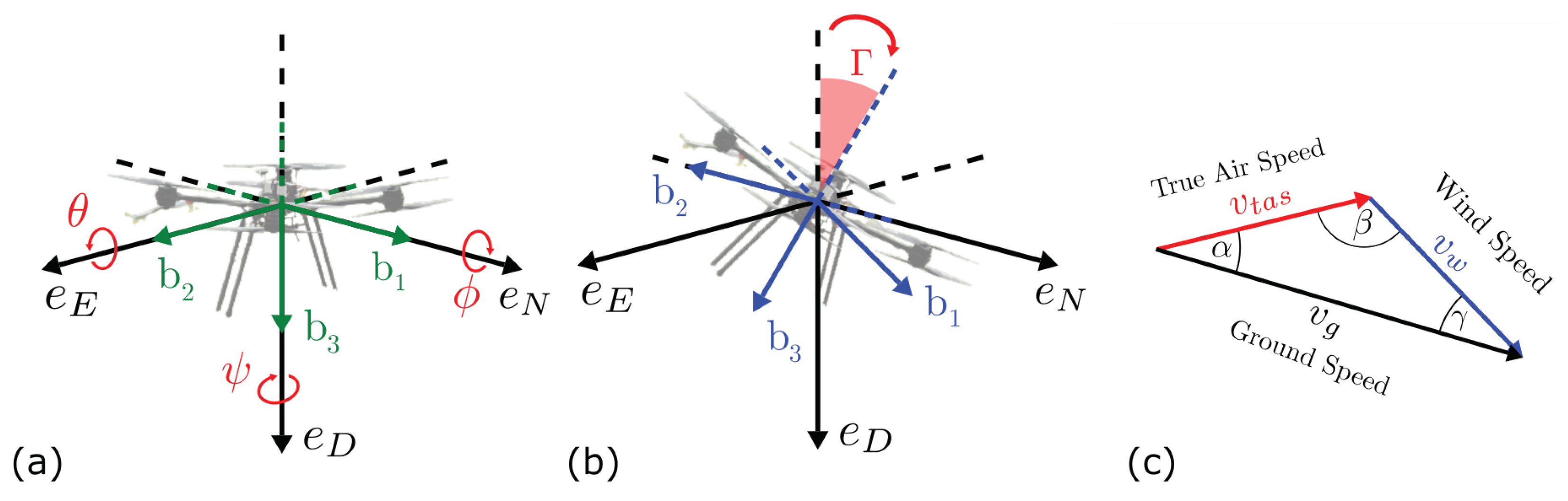
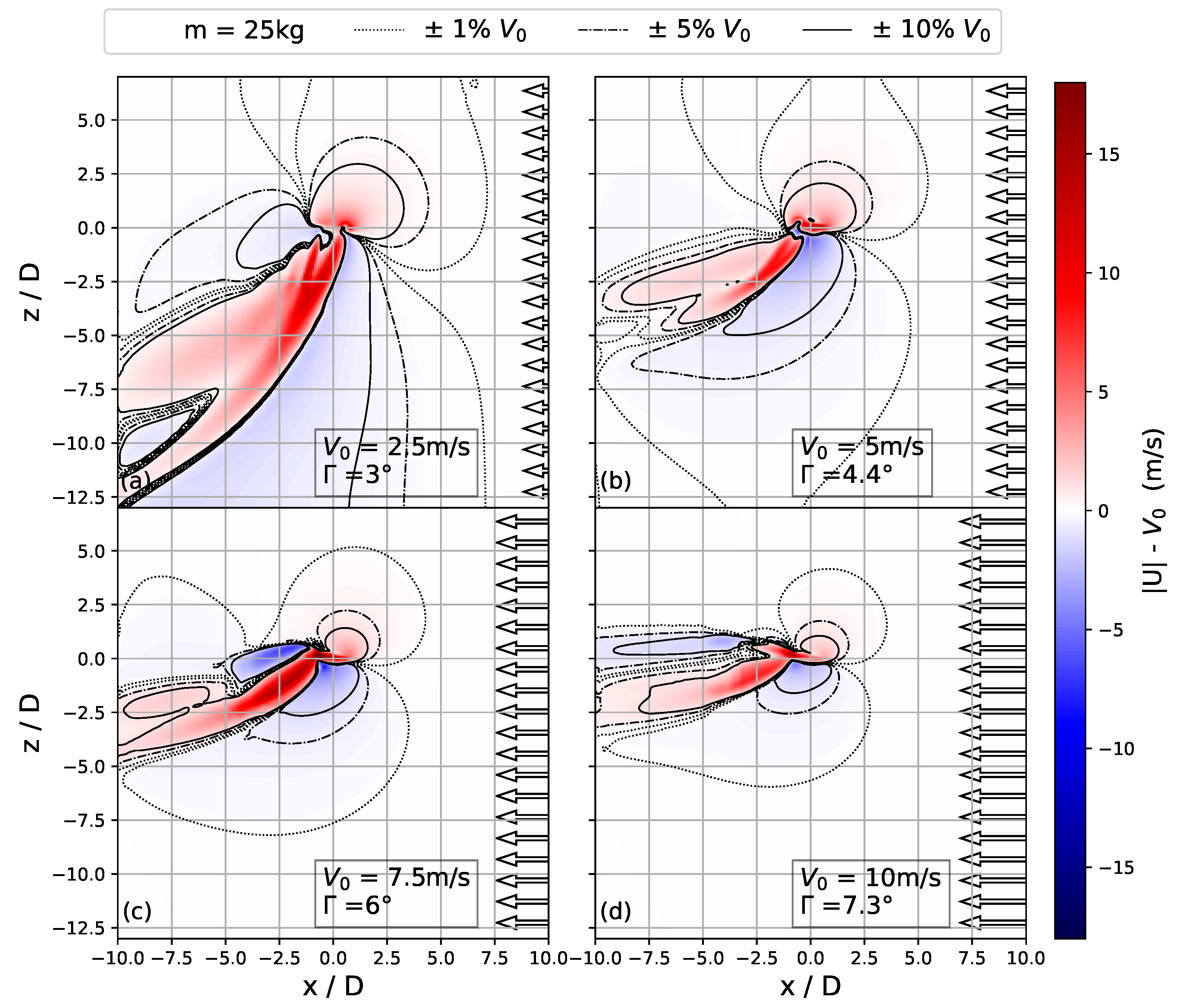
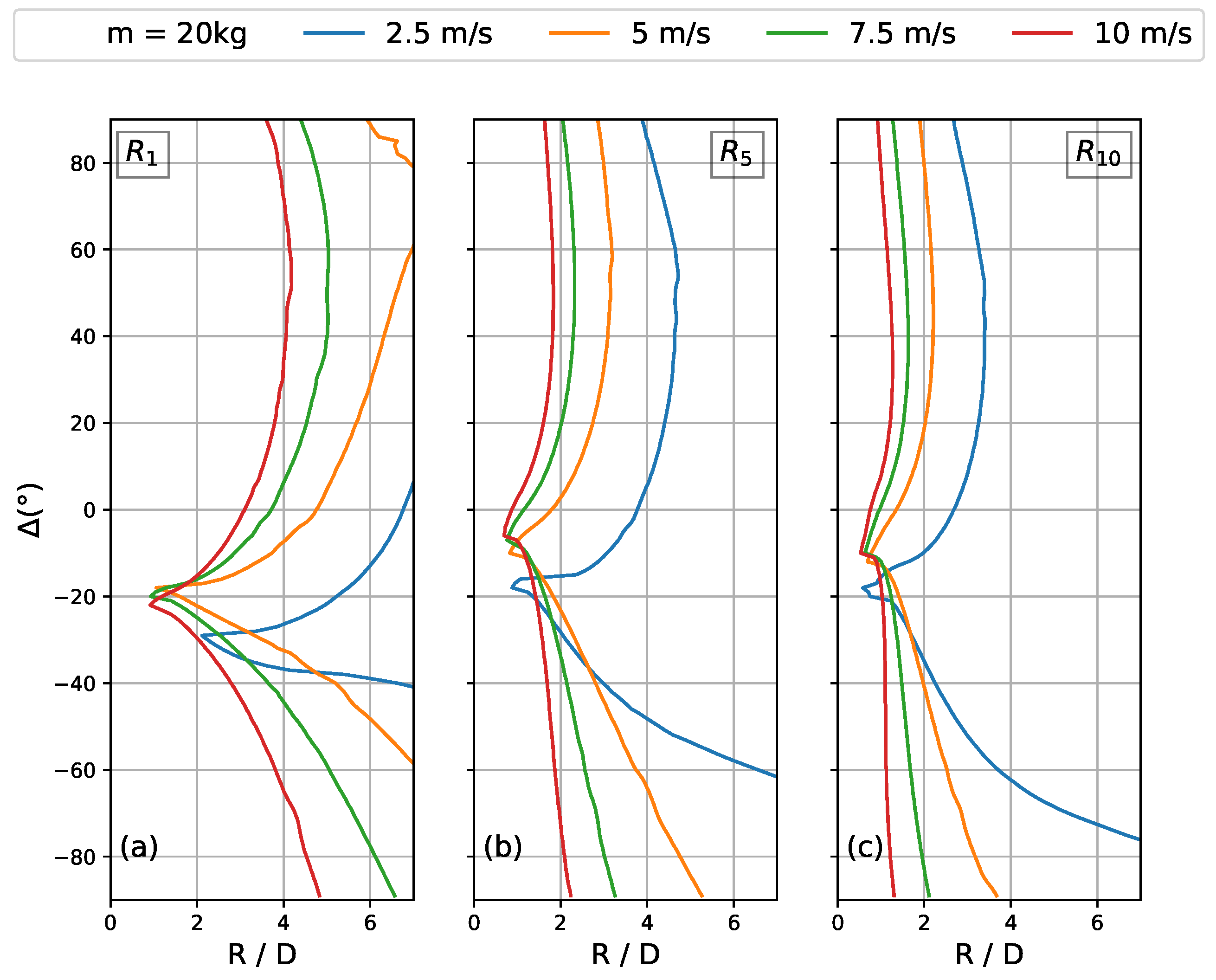
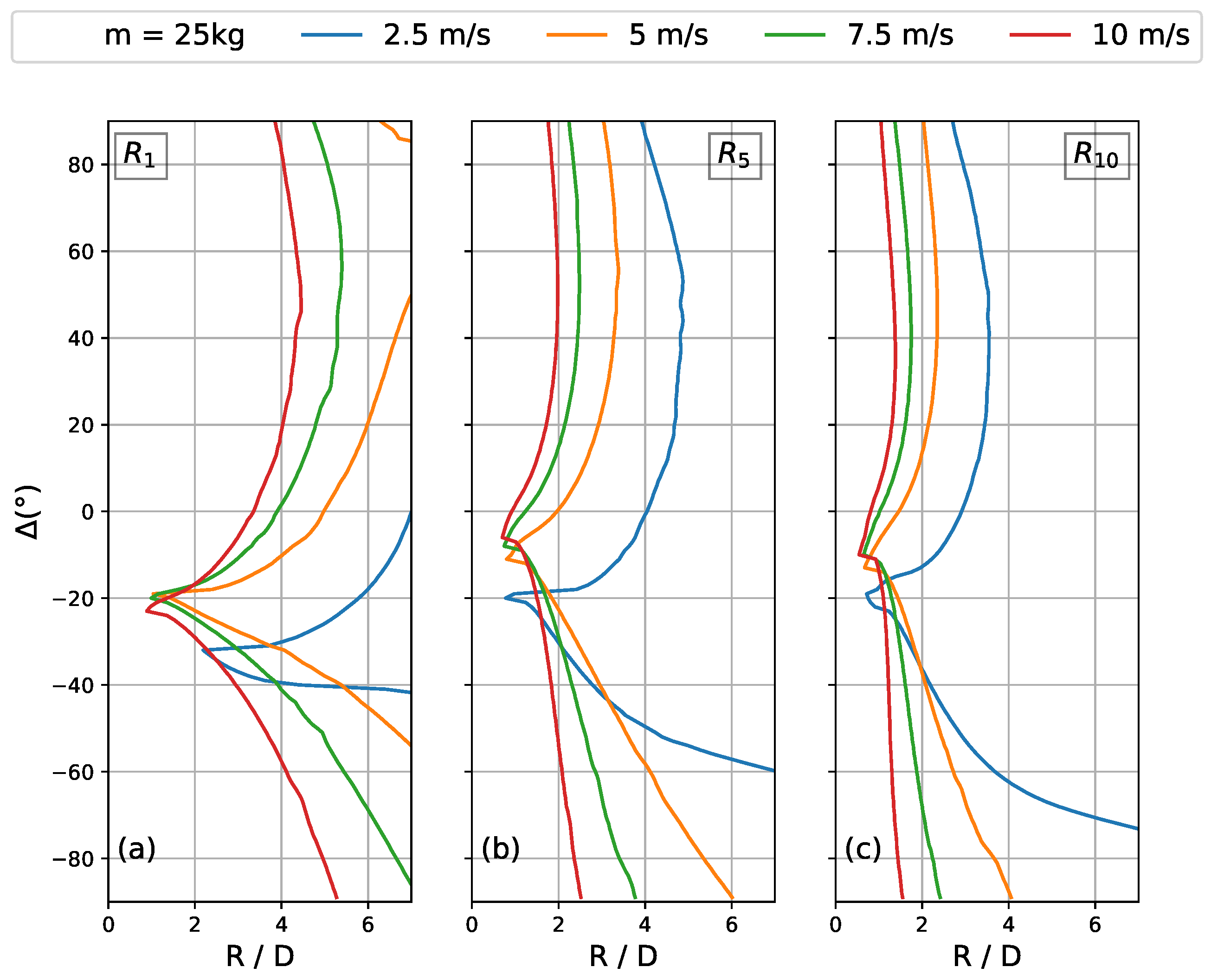
In this section, we define u, v, and w as the flow velocity components along the x, y, and z axis, respectively. The flow speed U is defined as $\sqrt{u^2+v^2+w^2}$. Since the results from the different weight configurations are qualitatively very similar and only vary in the vector magnitudes, only the results related to the 15 $\mathrm{kg}$ case are shown in this section. Results of the 20 kg and 25 $\mathrm{kg}$ cases are presented for completeness in Appendix A.2.

4.1. Propeller-Inducted Flow Features

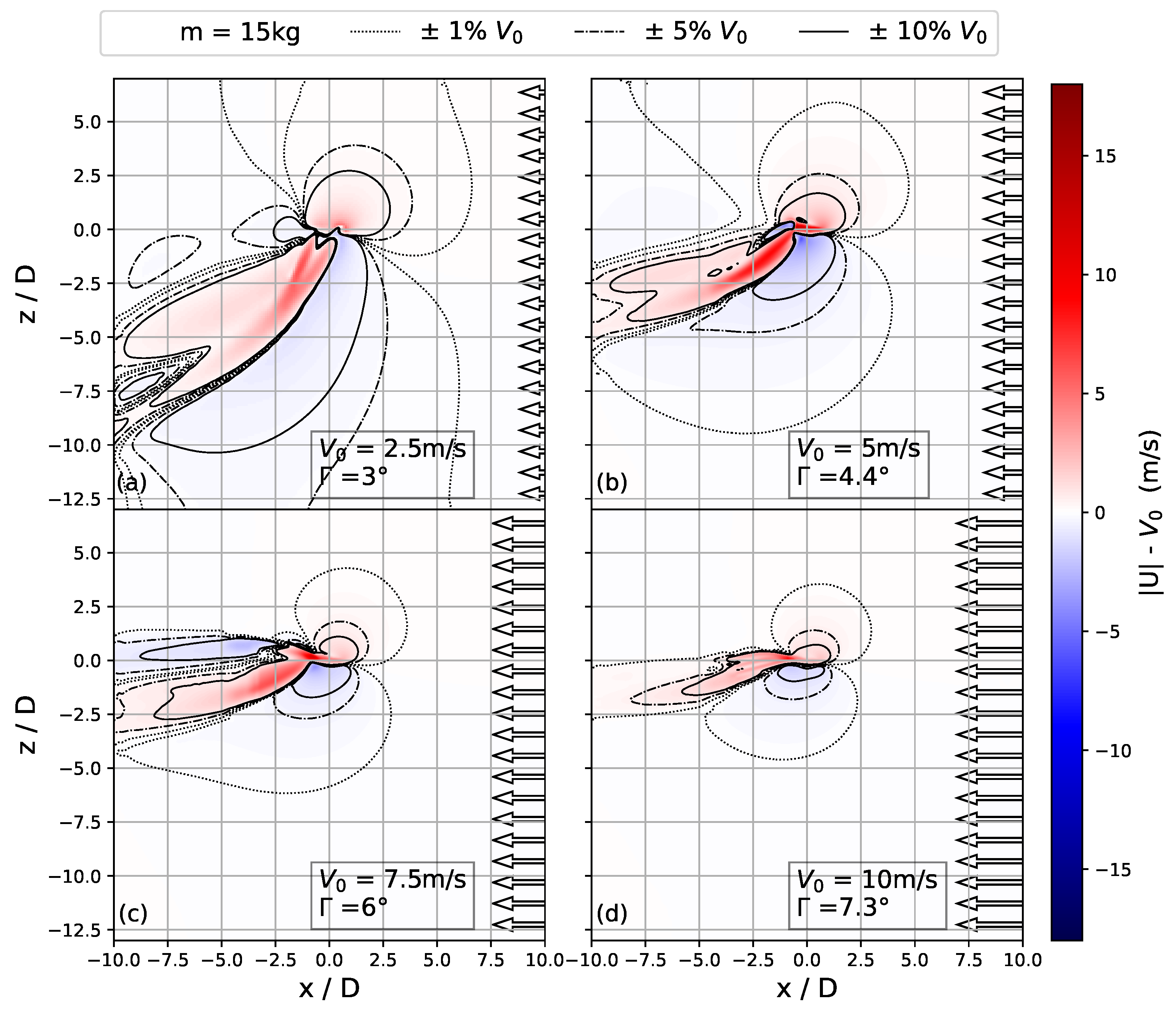
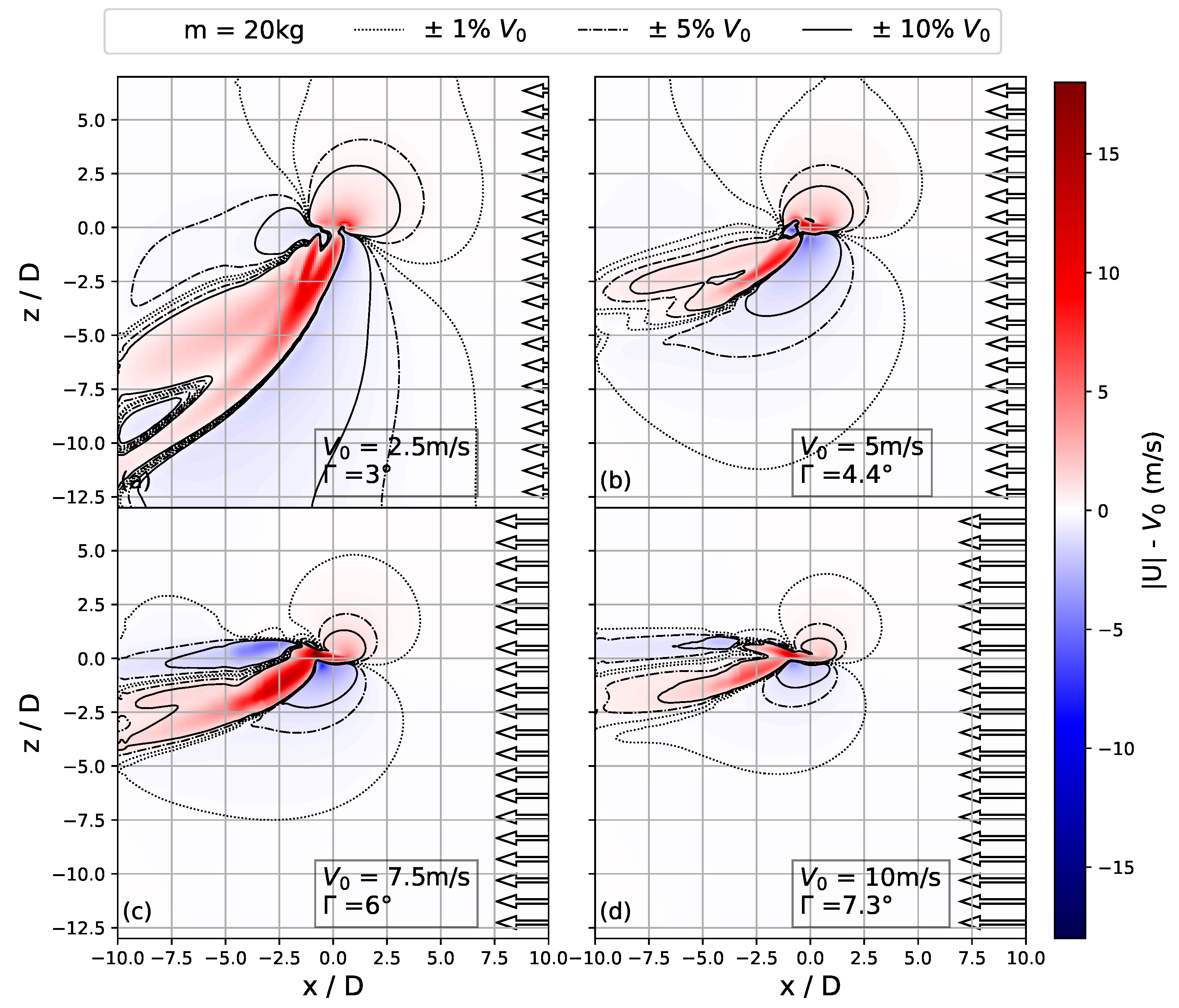
PIF features are described in terms of the deviation of the flow velocity components and flow speed from the background flow. For the sake of brevity, we refer to such deviations as delta flows. The spatial variation of delta flows is shown over vertical (xz-plane) and horizontal (xy-plane) cross-sections. Figure 7 shows |U| delta flow over vertical cross-sections (xz-plane, y = 0), and it features a panel for each of the inlet boundary inflow conditions (2.5 m s⁻¹, 5 m s⁻¹, 7.5 m s⁻¹ and 10 m s⁻¹).

The center of the UAV’s fuselage sits at (0,0,0), and the background flow is oriented from right to left. In the following, the color map scheme for the flow deviations (delta flows) is chosen in a way that the white color indicates a zero delta flow, while red and blue are associated with speed-up (positive delta flow) and slow-down (negative delta flow) with respect to the incoming wind field. All the panels share the same color grading. In addition, Figure 7 features dotted, dashed, and continuous contour lines that enclose areas with the absolute value of relative delta flow (delta flow over background flow) of 1%, 5% and 10%, respectively. Figure 7 shows that the PIF manifests both by flow acceleration and deceleration; these features are asymmetrically located both in the vertical and horizontal direction. The areas enclosed by the contour lines decrease as the background flow increases.

In general, the absolute delta flow values increase with the background flow. Maxima in delta flow are confined to an area between one rotor diameter above and three rotor diameters below the drone. The absolute maximum is reached in the $7.5$ m s⁻¹ case with a value of $11.7$ m s⁻¹ (16 m s⁻¹ and 17.9 m s⁻¹ in the 20 kg and 25 kg cases, respectively). Looking at the relative delta flow values, i.e., normalized by the background flow, the trend is reversed. The maximum relative delta value is found at $V_0$ = $2.5$ m s⁻¹ where |U| is 347% higher than the background flow in the 15 $\mathrm{kg}$ case and 425% higher for the 25 $\mathrm{kg}$ one. The minimum relative delta value is found in the 10 m s⁻¹ case, for |U| = 180% $V_0$ at 15 $\mathrm{kg}$ and |U| = 250% $V_0$.

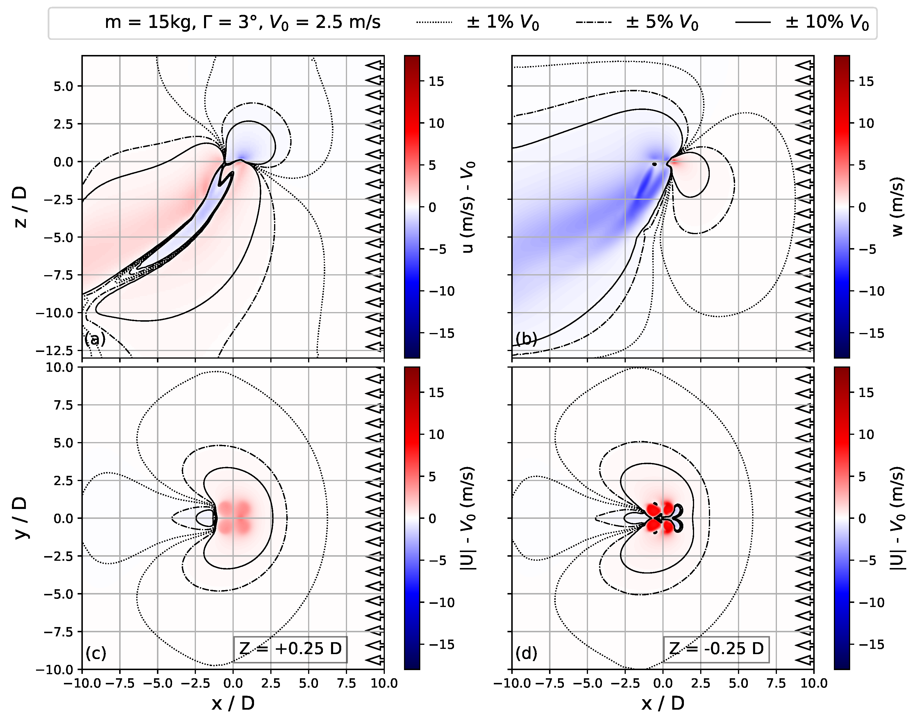
Figure 8 shows a more detailed picture of the three-dimensional flow structure around the UAV and focuses on the $V_0$ = $2.5$ m s⁻¹ case study. Figure 8a,b show vertical cross-sections (xz-plane at y/D = 0) of u and w delta flows, respectively. It is pointed out that the vertical component of the background flow is zero. Figure 8c,d feature |U| delta flow over horizontal cross-sections (xy-plane) at z = 0.25 D and z = −0.25 D in order. Figure 8’s design relies on the color scheme and contour lines previously presented in Figure 7.

Figure 7 and Figure 8c,d show that acceleration and deceleration features are found mostly below the rotor plane, whereas the flow above the rotor plane undergoes downward acceleration. Local flow decelerations are found in both downwind and upwind regions from the ADs, and they are from now on referred to as the wake and the induction zones, respectively. The wake is that part of the volume situated downwind, for negative x/D values, that sits behind the accelerated stream. In the wake, the flow experiences horizontal deceleration while being pushed downwards. The induction zone results from the interaction between the accelerated flow directed downwards and the background flow. It is located in the lower portion of the volume at z/D < 0 and x/D > 0. The induction zone below the mean rotor plane becomes wider with increasing distance, as it is shown in Figure 8c,d, and the flow running in this area is decelerated mainly in the horizontal component, as shown by Figure 8a,b.

4.2. Sensor Placement Study

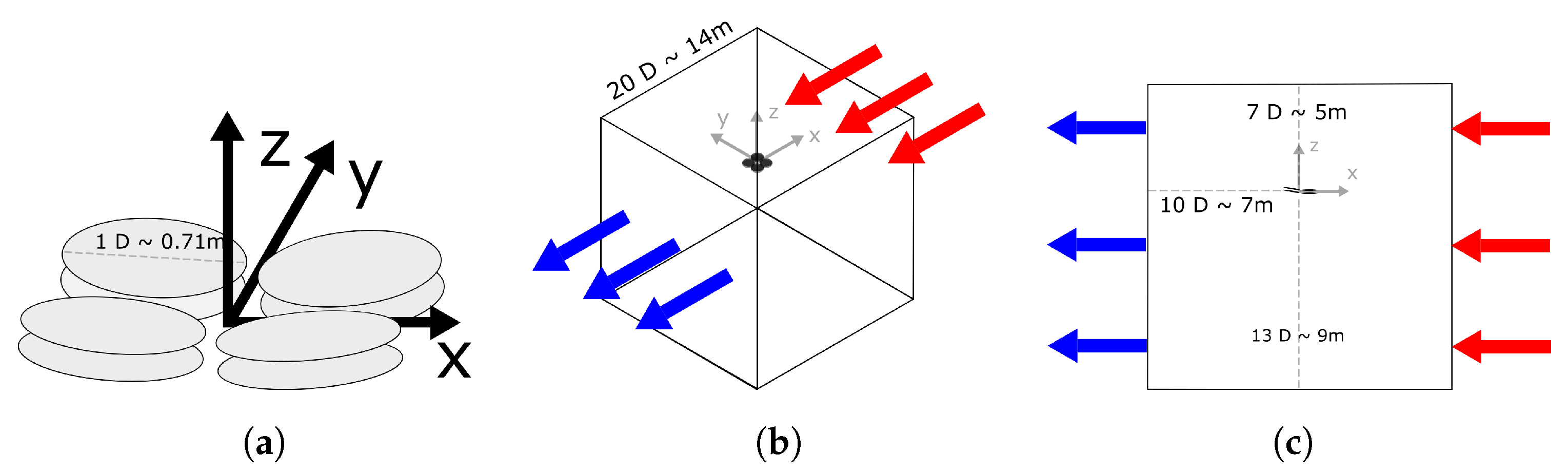
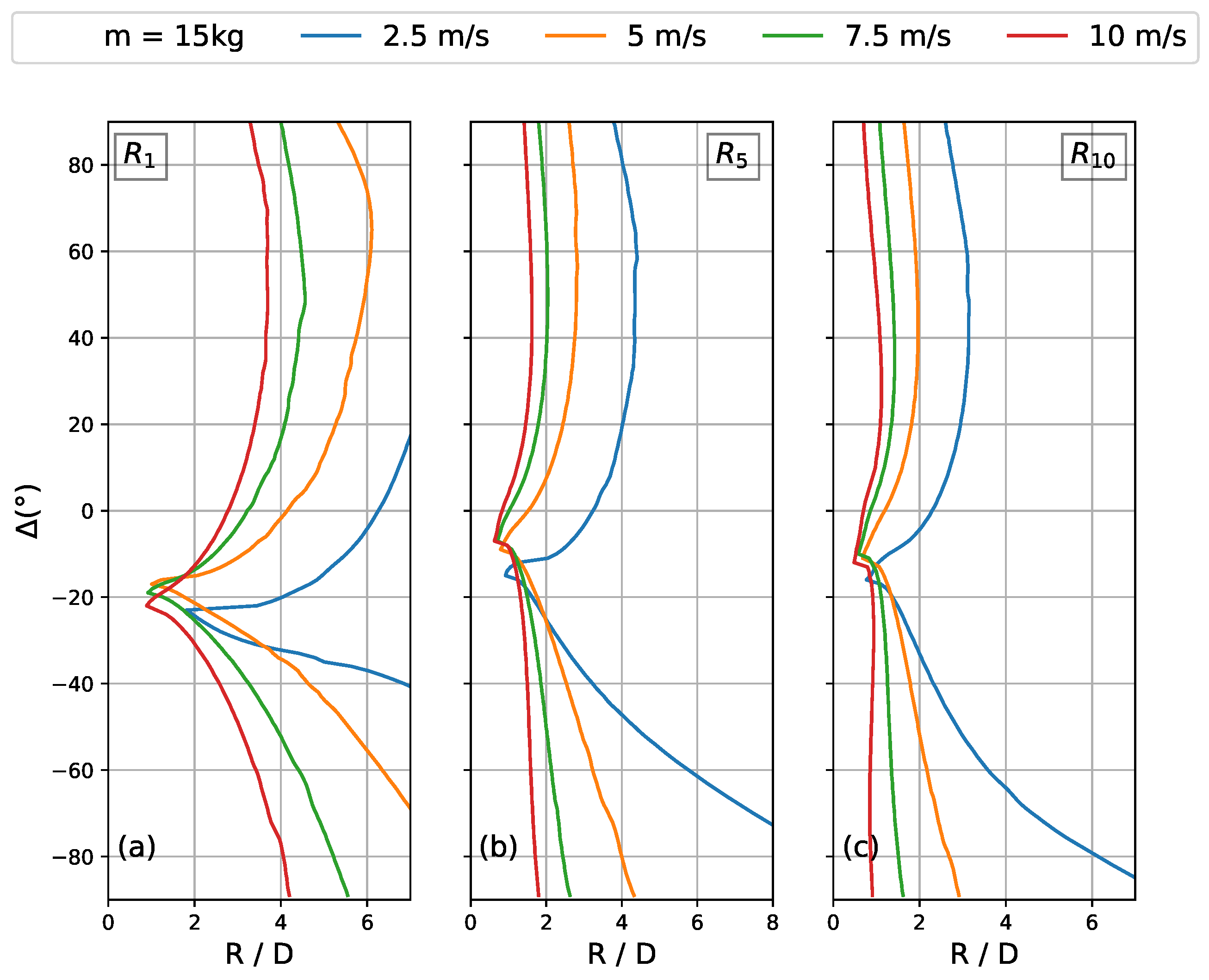
As mentioned in Section 1, this paper aims to evaluate where the PIF is minimal to identify suitable positions for turbulence measurements. Since the corresponding sensors are usually boom-mounted, we now investigate how long the sensor arm should be and in which direction it should point to minimize PIF effects on the turbulence measurements. Consequently, we now proceed with our analysis in a polar coordinate system that has its origin in the center of the drone. The downwind portion of the domain volume (x/D < 0) encloses the largest flow distortion and thus the highest flow variations. For this reason, it is discarded from further analysis. Figure 8c,d indicate that the flow is symmetric about the xz-plane that passes through the center of the coordinate system (y/D = 0). Mounting a sensor in this plane has the advantage of reducing the potential flow-inducted torques around the yaw axis. This increases the stability in flight, as well as increasing the operational time. Therefore, the PIF spatial variability in radial coordinates of the upstream portion of the xz-plane (x/D > 0, y/D = 0) is targeted for analysis. For this, we transform the contour lines previously presented in Figure 7 to a polar coordinates system that originates in the center of the fuselage and shares axes with the BF reference frame introduced in Section 2. Each point of the contour lines is described by R, the distance vector that origins in (0,0,0), and $\Delta$, the angle between R and ${\mathbf{b}}_1$. The $\Delta$ angle is defined as negative going towards ${\mathbf{b}}_3$ and varies from −90° to 90°, while the values of R are limited by the domain size. We define $R_1$, $R_5$, and $R_{10}$ as the 1%, 5%, and 10% delta flow contours lines in polar coordinates, accordingly. Results are presented in Figure 9. This figure is divided into three panels, each of which shows the distance threshold values for all the tested inlet speeds for the 15 kg case. Plots for the cases with 20 kg and 25 kg can be found in Appendix A.3.

Figure 9 shows that the $R/D$ values become smaller as the wind speed at the inlet increases. In other words, the higher the ambient wind speed, the shorter the required sensor arm length to reduce the PIF influence on the measurements. Changes in the mass of the drone are less relevant for the PIF than the changes of $V_0$; the biggest change due to mass variation for $R_1$ is found in the $7.5$ m s⁻¹ case: the average increase of $R/D$ values from the 15 $\mathrm{kg}$ to the 20 kg and 25 $\mathrm{kg}$ cases is 13% and 21%. On the contrary, changes in the variation of the wind speed $V_0$ between $2.5$ m s⁻¹ and 10 m s⁻¹ result in changes in $R/D$ values up to 80%. The results are compatible with previous experimental studies by e.g., Wilson et al. [51]. Despite using a UAV with propellers of $76.2$ mm mm diameter, i.e., roughly a factor of 10 smaller than ours, they come to a similar conclusion and showed that the PIF at 5.3 D (roughly 400 mm) above the UAV at the center of the fuselage, has negligible impact on the wind speed measurements. Wilson et al. compared high-frequency velocity data recorded by an ultrasonic anemometer (92,000, R.M. Young) on a mast to the one measured by a sonic anemometer (Trisonica Mini) mounted on a UAV at different vertical distances; they show a deviation of the mean wind speed between these two measurements of 0.7%, 5.5%, and −1.8% at 5.3 D, 6.6 D, and 8 D accordingly. Our results show that in the worst-case scenario (Figure A4), on top of the UAV ($\Delta$ = 90°) at a distance between 3.9 D and 7 D, the flow undergoes an absolute distortion in between 1% and 5%. Prudden et al. [19] measured the PIF of a UAV with a propeller size of 330 mm. They did so in a wind tunnel set-up varying the inlet flow from 4 m s⁻¹ up to 8 m s⁻¹, focusing on the upwind flow distortion in terms of flow angle deflection and flow speed. They show that the flow angle undergoes a deflection of fewer than 2 degrees at 3.35 D along ${\mathbf{b}}_1$. So, it is still possible to measure PIF at that distance. Nevertheless, they concluded that this distortion is so small that it can be neglected. In addition, they point out that mounting a sensor more than 3.5 D towards ${\mathbf{b}}_1$ to avoid all induced flow effects is not a feasible solution with respect to flight stability. Consequently, it is necessary to find a feasible compromise. Prudden et al. [19] suggest 1.25 D towards ${\mathbf{b}}_1$ as a reasonable mounting distance since the flow in that position is characterized by an acceleration of less than 2% and an angle distortion of fewer than 2°. According to our results, a distance of 3.95 D and 3.4 D along ${\mathbf{b}}_1$ would suffice to measure a distortion of 1% at $7.5$ m s⁻¹ and 10 m s⁻¹, accordingly, and a distance of 1.3 D and 0.98 D for a 5% one. The results presented in Figure 9 show that, in general, the smallest values of $R/D$ are found in a range of $\Delta$ angles that varies from −10° to −23°. This suggests that moving the sensor upwind, along a horizontal plane lower than the one that passes through the center of the related fuselage, is the more efficient way to reduce the relative PIF influence on the measurements. For each curve presented in Figure 9, among all the ($R/D$, $\Delta$) points in that curve, we define the closest one to the fuselage as ($R_{best}/D$, ${\Delta }_{best}$).

Table 5. Comprehensive values list of the m = 15 kg configuration case for the threshold distance curves $R_1$, $R_5$, $R_{10}$. $R_{best}$ and $\Delta$ are the polar coordinates of the minimum distance in a specific threshold-velocity inlet configuration, whereas $z_{BF}$ and $x_{BF}$ are the projection of $R_{best}$ over the UAV reference frame.

	${\mathit{V}}_0$ (m ${\mathbf{s}}^{-1}$)	${\mathbf{\Delta }}_{\mathit{best}}$ (°)	${\mathit{R}}_{\mathit{best}}/\mathit{D}$	${\mathit{R}}_{\mathit{best}}$ (m)	${\mathit{z}}_{\mathit{BF}\mathit{best}}$ (m)	${\mathit{x}}_{\mathit{BF}\mathit{best}}$ (m)
$R_{10}$:	2.5	−16	0.77	0.55	0.15	0.52
	5.0	−11	0.67	0.48	0.09	0.47
	7.5	−10	0.57	0.40	0.07	0.40
	10	−12	0.48	0.34	0.07	0.33
$R_5$:	2.5	−15	0.91	0.65	0.17	0.62
	5.0	−9.0	0.80	0.56	0.08	0.55
	7.5	−7.0	0.71	0.50	0.06	0.50
	10	−7.0	0.63	0.44	0.05	0.44
$R_1$:	2.5	−23	1.81	1.29	0.50	1.18
	5.0	−17	1.00	0.71	0.20	0.68
	7.5	−19	0.92	0.65	0.21	0.61
	10	−22	0.88	0.62	0.23	0.57

lists, for each threshold distance curve, and for each tested inlet velocity, the minimal distance points coordinates ($R_{best}/D$, ${\Delta }_{best}$), the radial distance in meter $R_{best}$, and its projections onto the ${\mathbf{b}}_1$ and ${\mathbf{b}}_3$ BF reference frame vectors, called $x_{BFbest}$ and $z_{BFbest}$, respectively.

Table 5 shows that the ($R_{best}/D$, ${\Delta }_{best}$) points sit in a 0.48–1.81 D distance range from the fuselage, at an angle that varies in between −7° and −23°. This corresponds to a 0.46–1.66 D range along $x_{BF}$, and a 0.01–0.7 D range along $z_{BF}$. Therefore, the suitable position for a turbulence-sampling sensor, e.g., ultrasonic anemometer, is not universal and depends both on the acceptable PIF threshold for a given application and the ambient flow conditions.

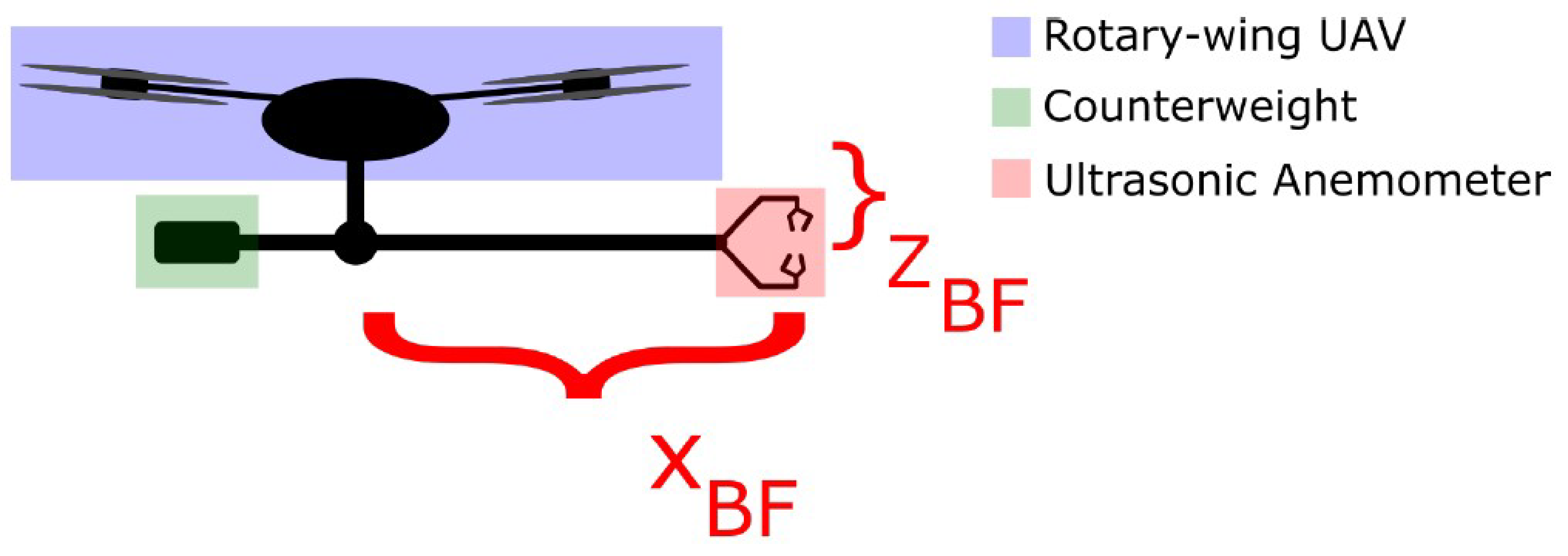
Based on the results shown in this paper, we now introduce a design of a boom-mounted ultrasonic anemometer that aims to sample turbulence in offshore wind farms. The design is named SAMURAI, which stands for “sonic anemometer on a multi-rotor drone for atmospheric turbulence investigations”. Figure 10 presents a sketch of the SAMURAI system.

In this design, an ultrasonic anemometer is installed on the tip of a horizontal boom pointed upwind, at a horizontal sensor mounting distance of $x_{BF}=1.7$ m, and a vertical one of $z_{BF}=0.2$ m from the center of the fuselage in the BF reference frame. The asymmetry in the weight distribution is compensated by a counterweight mounted on the other end of the boom. The choice for $x_{BF}$ and $z_{BF}$ is justified as follows:

• Since relevant velocities in the wind energy field are higher than 5 m s⁻¹, the results related to the $2.5$ m s⁻¹ case study were not given priority over the choice of $x_{BF}$ and $z_{BF}$;
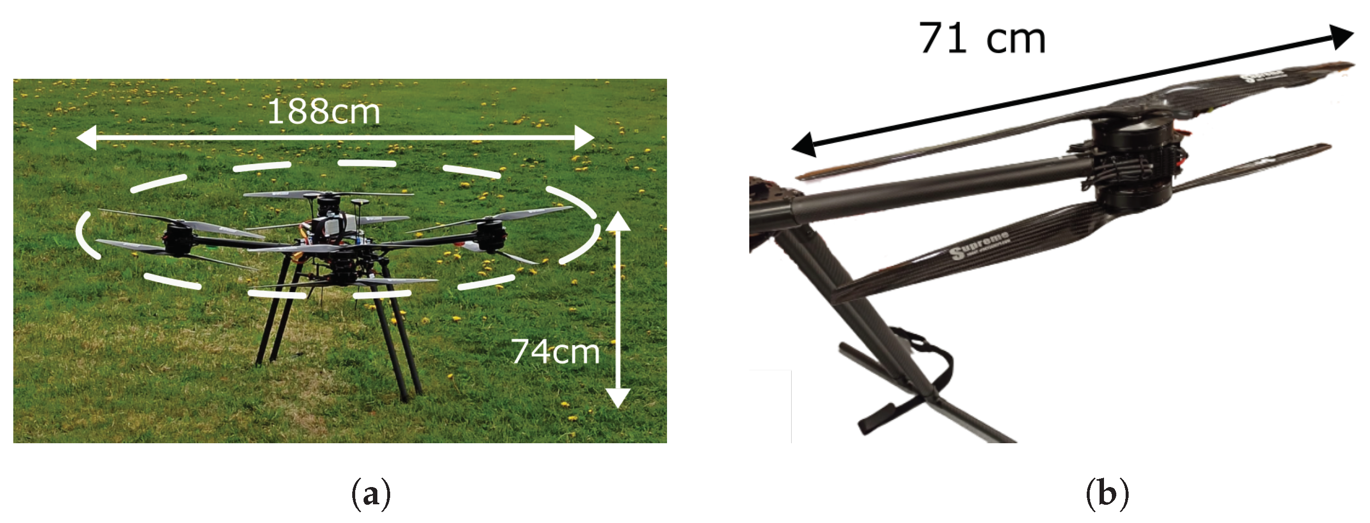
• The total height of the tested UAV (74 cm) puts a limit on the vertical mounting distance of the boom. To increase safety during the landing phase we decided not to lower the boom more than 20 cm from the center of the fuselage. By doing this, we assure a safety distance of 44 cm between the boom and the ground;
• The size of the tested UAV (overall diameter from rotor-tip to rotor-tip 188 cm) puts a limit on the horizontal displacement of the sensor as well. In case of a faulty landing, having the sensor mounted at a horizontal distance higher than the UAV radius, $x_{BF}>94 \mathrm{cm}$, can reduce the damage to the system. The results shown in Table 5 suggest that, for the set-up presented in this paper, a horizontal sensor-mounting distance $x_{BF}=1.7$ m would be enough to measure wind with a |U| delta flow in between 5% and 10% for $V_0$ = $2.5$ m s⁻¹, and less than 1% for all the other case studies. In absolute terms, this means a deviation in between $0.12$ m and $0.25$ m for $V_0$ = $2.5$ m s⁻¹, and less than 0.05 m s⁻¹, 0.075 m s⁻¹ and 0.1 m s⁻¹ for the 5 m s⁻¹, 7.5 m s⁻¹ and 10 m s⁻¹ case, accordingly.

Finally, an in-depth list of flow features averaged around a 10 cm radius circle around the mounting position ($x_{BF}$ = $1.7$ m, $z_{BF}$ = $0.2$ m), is presented in

Table 6. Averages of overall flow speed ($\overline{U}$), horizontal ($\overline{u+v}$) and vertical flow speed ($\overline{w}$), and flow angle (Angle) ± standard deviation ($\sigma$), around a 10 cm radius circle with center at the mounting position ($x_{BF}$ = $1.7$ m s⁻¹, $z_{BF}$ = $0.2$ m s⁻¹) for different inlet velocities $V_0$.

Payload (kg)	${\mathit{V}}_0$ m ${\mathrm{s}}^{-1}$	$\overline{\mathit{U}}$ m ${\mathrm{s}}^{-1}$	$\overline{\mathit{u}+\mathit{v}}$ m ${\mathrm{s}}^{-1}$	$\overline{\mathit{w}}$ m ${\mathrm{s}}^{-1}$	Angle (°)
15	2.5	2.6 ± 0.1	2.6 ± 0.1	0.4 ± 0.1	9.1 ± 4.2
	5.0	5.0 ± 0.1	5.0 ± 0.1	0.3 ± 0.1	3.5 ± 1.7
	7.5	7.5 ± 0.1	7.5 ± 0.1	0.2 ± 0.1	1.8 ± 0.9
	10	10 ± 0.1	10 ± 0.1	0.2 ± 0.1	1.1 ± 0.5
20	2.5	2.6 ± 0.2	2.6 ± 0.2	0.5 ± 0.2	10.4 ± 4.9
	5.0	5.0 ± 0.1	5.0 ± 0.1	0.4 ± 0.1	4.5 ± 2.1
	7.5	7.5 ± 0.1	7.5 ± 0.1	0.3 ± 0.1	2.4 ± 1.1
	10	10.0 ± 0.1	10 ± 0.1	0.3 ± 0.1	1.4 ± 0.7
25	2.5	2.7 ± 0.2	2.7 ± 0.2	0.5 ± 0.2	11.1 ± 5.2
	5.0	5.0 ± 0.2	5.0 ± 0.2	0.4 ± 0.2	5.1 ± 2.4
	7.5	7.5 ± 0.1	7.5 ± 0.1	0.4 ± 0.1	2.7 ± 1.3
	10	10.0 ± 0.1	10.0 ± 0.1	0.3 ± 0.1	1.7 ± 0.8

.

The listed values show that at the designed coordinates, the flow is tilted upwards with an angle that decreases as the background flow increases. The flow angle values are lower than 11.1° ± 5.24°, and so they are within the acceptable measuring range of most ultrasonic anemometers, e.g., CSAT3B by Campbell Scientific. Moreover, the aforementioned anemometer has a nominal maximum gain error ±3% when reading a wind vector within ±10° angle from the horizontal plane, that is a bigger error range than the bias due to the PIF influence. For this reason, the ($x_{BF}$ = $1.7$ m, $z_{BF}$ = $0.2$ m) is considered to be a suitable mounting spot for turbulent sampling instruments.

5. Conclusions

This paper investigates the flow field around a large multi-copter and the interaction of the mean flow with the propeller-induced flow (PIF). The goal is to determine suitable positions for the integration of turbulence-resolving measurement systems. We used computational fluid dynamic(CFD) simulations to investigate the spatial distribution of PIF generated by a multi-copter with coaxial contra-rotating propellers and a propeller size of $0.71$ m. To provide a realistic tilt angle of the UAV in the CFD simulations, several flight tests were conducted to get an estimation of the UAV’s attitude angle as a function of the wind speed under stationary flight conditions. Then, steady-state CFD simulations were carried out using the commercial software Ansys Fluent 2022 R1, running RANS equations with $k-\epsilon$ turbulence closure model and actuator disc theory. Four different inlet velocities (2.5 m s⁻¹, 5 m s⁻¹, 7.5 m s⁻¹ and 10 m s⁻¹), and three weight configurations (15 kg, 20 kg and 25 $\mathrm{kg}$) were tested.

The results indicate that the PIF influences the surrounding flow with both asymmetrical acceleration and deceleration features in both vertical and horizontal directions. The portion of the domain that is the least affected by the PIF is the region situated upstream of the UAV. The results show that from the center of the fuselage, at a vertical distance between 3.9 D and 7 D, the flow undergoes a distortion of 1% and 5%. In addition, a horizontal distance of more than 3.95 D in the upwind direction from the center of the fuselage would suffice to measure a distortion of less than 1% with an inlet velocity of more than $7.5$ m s⁻¹. These results are comparable to what is found in the literature. The results also show that the best suitable position for turbulence-sampling sensors is not unique and it lies in a range of 0.46–1.66 D upwind from the main fuselage and 0.01–0.7 D below the mean rotor plane. These ranges depend on the choice of inlet and relative flow distortion level 1%, 5%, and 10%.

Based on the obtained results, the paper proposes a well-balanced compromise between flow distortion and flight stability. In the presented set-up, a sensor mounted at $x_{BF}$ = $1.7$ m (horizontal distance), and $z_{BF}$ = 20 cm (vertical distance under the UAV) undergoes a PIF in between 5% and 10% in a $2.5$ m s⁻¹ wind flow and becomes less than 1% for all the other cases studied (5 m s⁻¹, 7.5 m s⁻¹ and 10 m s⁻¹). This means an absolute deviation between $0.12$ m and $0.25$ m for $V_0$ = $2.5$ m s⁻¹, and less than 0.05 m s⁻¹, 0.075 m s⁻¹ and 0.1 m s⁻¹ for the 5 m s⁻¹, 7.5 m s⁻¹ and 10 m s⁻¹ case, accordingly. These deviations are within the acceptable measuring range of most ultrasonic anemometers, e.g., CSAT3B by Campbell Scientific.

The presented methodology in this paper offers the advantage of low computational cost and simplified geometry, reducing the required workload. It serves as an investigative tool for understanding the general features of the PIF. However, it is crucial to validate the results presented herein through comparison with full-scale experiments. Ongoing experimental tests are being conducted, and their findings will be the subject of future follow-up publications.