Tracking a Maneuvering Object by Indirect Observations with Random Delays

Abstract

A mathematical model for the target tracking problem is proposed. The model makes it possible to describe conditions when the time for an observer to receive the results of indirect observations of a moving object depends not only on the state of the observation environment but also on the state of the object itself. The source of such a model is the observation process, by stationary means, of an autonomous underwater vehicle, in which the time for obtaining up-to-date data depends on the unknown distance between the object and the observer. As part of the study of the problem, the equations of the optimal Bayesian filter are obtained. But this filter is not possible to implement. For practical purposes, it is proposed to use the conditionally minimax nonlinear filter, which has shown promising results in other complex tracking models. The conditions for the filter’s evaluation and its accuracy characteristics are given. A large-scale numerical experiment illustrating the filter’s operation and the observation system’s features with random delays are described.

1. Introduction

The problem of tracking a maneuvering object using a model with random factors is a typical application of stochastic filtering theory and methods [1]. In addition to navigation, these methods are widely used in other areas, sometimes entirely unexpectedly, such as medicine, industry, economics, and telecommunications [2,3,4,5,6,7]. The model and problem statement discussed in the article are inspired by the popular modern applied field of autonomous underwater vehicles (AUVs) [8]. Many works are devoted to AUV applications, most of which are related to control tasks. The special issue of [9] sufficiently illustrates the scope and magnitude of the research interest in this area. Moreover, let us pay attention to the fact that researchers use many new methods as tools, primarily due to the development of machine learning (a typical example is work [10], and there are many such works [11]). At the same time, the conventional tasks of target tracking remain in demand; one can find many new and exciting things in them [12,13,14,15,16,17,18,19,20]. Here it is necessary to note the tasks of tracking multiple targets [21,22], the solution of which, as well as conventional statements, is provided by stochastic filtering methods.

The Kalman filtering model, algorithm [23], and many different suboptimal filters have become widely used. The simplest algorithms of this kind, starting with the extended Kalman filter [24] and modern developments of the odorless or cubature Kalman filters [25,26,27], can be effective in individual applications. Such ideas have found many applications and options for development/improvement. An excellent attempt to systematize the results in this area was made in [28]. To date, many more works have appeared devoted to the research and improvement in such suboptimal filters [29,30,31,32], including those applied to target tracking tasks of AUVs [33]. However, no fundamentally new ideas have been proposed, and the initially existing shortcomings remain. The essence of these disadvantages is that none of these filters guarantees accurate characteristics for at least any broad class of models. That is, the estimates do not guarantee either the absence of bias or the limitation of the error, at least by the variance of the estimated state. This means there is always a danger that the filter will be unstable in another model and the estimate will diverge. The only guarantee is a practical experiment with a specific model and a fixed set of parameters.

It should be noted that the problem of delayed observations is well known in the field of application under discussion. Such delays are due to a prominent characteristic of acoustic meters: the dependence of the acoustic wave propagation velocity on temperature, salinity, and water pressure [34]. This attracted attention in the above-mentioned study [20], and a solution was found by combining measurement data from acoustic sensors with information from other sensors in the onboard inertial navigation system. A more typical way to deal with delayed observations is to estimate the delay time and consider it by adjusting the usual filter [35]. Interestingly, the delay in observations is explained by nature not only for underwater observations but also in some chemical processes [36].

It should be understood that models with a deterministic delay time have limited use because, in reality, the delay time is random and significantly depends on the observation conditions, and most importantly, it changes during tracking. Moreover, these changes can be significant. In the model proposed in this article, the time delay of observations is described by a random process, which is a known function of the state of the observation system. Such a description of delays makes the model as adequate as possible when describing the results of the acoustic sensors.

At the same time, formally, the model of the observation system remains a Markov process model with discrete time. Hence, the classical Bayesian filtering procedure can be applied to it [37], i.e., obtaining recurrent relations for the a posteriori probability density is possible. The next section of the article shows these relations. However, this formal success turned out to be relevant only to justify the impossibility of practical implementation of either the optimal filter itself or its suboptimal simplifications. The reason for this is that the formal reduction of the equations of the observation system to the traditional form enormously increases the dimension.

An alternative to suboptimal filters is the conditionally minimax nonlinear filtering (CMNF) [38]. Initially and in development [39], this method focused on applications in aircraft tracking tasks, which remain relevant for modern tasks [40]. However, the same approach has shown effectiveness in specific tasks for AUVs. So, in [19], an already modified CMNF for tracking underwater vehicles was shown, but with an emphasis on the efficiency of using Doppler sensors. It turned out that the CMNF algorithm does not require refinement for the proposed model with random delay. It is only necessary to clarify the conditions of existence. Section 3 of the article contains the statement required.

It turned out to be more challenging to adapt the typical filter structure to the task of AUV tracking. A standard filter structure using a prediction via a system state model and a correction in the form of a residual did not show good results when processing the acoustic observations. Nevertheless, the flexibility of the CMNF method made it possible to adjust the filter structure, consider the physical properties of observers, and obtain a very effective estimate as a result. Within the framework of the numerical experiment presented in Section 4 of the article, we show the process of physically justified adjustments to the filter structure. Section 5 contains concluding remarks, including considerations on options for further development of the proposed method.

2. Observation System Model and Optimal Filtering

The model uses discrete time. It is assumed that the filtering process, i.e., the calculation of the first state estimate, begins at the moment $t=0$. The maximum possible delay is known and is equal to $T$; therefore, the state of the system $x_t$ begins to form at the moment $t=-T.$ Thus, $t=-T,-T+1,\dots ,0,1,\dots ,$ and the initial state is set at the moment $-T-1$. Three variants of recording the equations of the observation system are considered. The first one has the most general form:

$$\begin{array}{c}{x}_t={\phi }_t\left(x_{t-1},w_t\right), x_{-T-1}=\eta ,\\ y_t={\psi }_t\left(x_{t-{\tau }_t},v_t\right), {\tau }_t={\theta }_t\left(x_t\right).\end{array}$$

(1)

The second version of the recording is a discrete analog of the diffusion process:

$$\begin{array}{c}{x}_t={\phi }_t\left(x_{t-1}\right)+{\phi }_t^w\left(x_{t-1}\right)w_t, x_{-T-1}=\eta ,\\ y_t={\psi }_t\left(x_{t-{\tau }_t}\right)+{\psi }_t^v\left(x_{t-1}\right)v_t, {\tau }_t={\theta }_t\left(x_t\right).\end{array}$$

(2)

The latter version is the most particular, but the most frequently used. This model is used by many suboptimal filters. It is also the most convenient for optimal Bayesian filtering. The system with state-independent noise is written as follows:

$$\begin{array}{c}{x}_t={\phi }_t\left(x_{t-1}\right)+w_t, x_{-T-1}=\eta ,\\ y_t={\psi }_t\left(x_{t-{\tau }_t}\right)+v_t, {\tau }_t={\theta }_t\left(x_t\right).\end{array}$$

(3)

In (1)–(3) $x_t\in {\mathbb{R}}^{p_x}$ represents the system state vector; $w_t\in {\mathbb{R}}^{p_w}$ is the discrete white noise modeling perturbations of the system; $\eta \in {\mathbb{R}}^{p_x}$ is the initial state vector; $y_t\in {\mathbb{R}}^{q_y}$ is the vector of indirect observations; $v_t\in {\mathbb{R}}^{q_v}$ is the discrete white noise modeling measurement errors; vectors $\eta ,w_t,v_t$ are assumed to be independent in aggregate. The model of observations delays, ${\tau }_t$, is given by a vector of the same dimension as the observations themselves. The elements of the vector, ${\tau }_t\in {\mathbb{R}}^{q_y}$, set the time delays for the corresponding components of the vector $y_t.$ Namely, each component ${\left({\tau }_t\right)}_i$ is a random sequence with values in the set $\left\{0,1,\dots ,T\right\}$, i.e., ${\left({\tau }_t\right)}_i\in \left\{0,1,\dots ,T\right\}$ for $i=1,\dots ,q_y.$ We consider $x_{t-{\tau }_t}$ as a composite vector containing the states $x_t$ with all the shifts ${\left({\tau }_t\right)}_i$, i.e., $x_{t-{\tau }_t}={\left(x_{{t-\left({\tau }_t\right)}_1}^{\prime },\dots ,x_{{t-\left({\tau }_t\right)}_{q_{y_{}}}}^{\prime }\right)}^{\prime }$. This notation makes accurate (1)–(3) and further relations.

The problem of estimating the state $x_t$ from observations $y_s,s=0,1,\dots ,t$, is considered, and the evaluation accuracy criterion ${\widehat{x}}_t$ is the mean square, i.e., $\mathrm{E}\left\{{‖x_t-{\widehat{x}}_t‖}^2\right\},\mathrm{E}\left\{x\right\}$ is the mathematical expectation of the vector $x$, and $‖x‖$ is the usual Euclidean norm of the vector $x$.

Thus, the random observation delay (${\tau }_t$) is the only difference between the considered problem statement and the traditional one of filtering the state of the observation system in discrete time. This difference does not exist formally because the following shows how to bring systems (1)–(3) into the traditional recording form. Therefore, the optimal solution is a conditional mathematical expectation of $x_t$ relative to observations $y_s,s=0,1,\dots ,t.$ So, it is enough to know the a posteriori probability density of $x_t$ relative to $y_s,s=0,1,\dots ,t$. Next, the a posteriori density for system (3) and $t=0,1,\dots ,$ will be written out in the form of recurrent Bayesian relations [37] under conditions when the necessary probability densities exist, i.e., under certain restrictions on the continuity of nonlinear functions and perturbations in (3). We avoid unnecessarily cumbersome relations with no practical value by limiting the discussion of the optimal filter to the system (3). For formal conclusions, system (3) is sufficient.

The non-Markov observation system (3) can be written as a Markov process with an extended state vector. Formally, this extended process will have the same form (3), but with ${\tau }_t=0.$

The extended state vector is further denoted by ${\mathbf{x}}_t\in {\mathbb{R}}^{\left(T+1\right)p_x}$ and is a composite vector, consisting of all the states of the system from time $t-T$ to the current moment $t$, i.e., ${\mathbf{x}}_t={\left(x_{t-T}^{\prime },\dots ,x_{t-1}^{\prime },x_t^{\prime }\right)}^{\prime }$. The notation $\prime$ is used here for the transpose operation. The equation for ${\mathbf{x}}_t$ has the following form:

$$\begin{array}{c}{\left({\mathbf{x}}_t\right)}_1^{p_x}={\left({\mathbf{x}}_{t-1}\right)}_{p_x+1}^{2p_x},\\ \dots \\ \begin{array}{c}{\left({\mathbf{x}}_t\right)}_{\left(T-1\right)p_x+1}^{T{p}_x}={\left({\mathbf{x}}_{t-1}\right)}_{T{p}_x+1}^{\left(T+1\right)p_x},\\ {\left({\mathbf{x}}_t\right)}_{T{p}_x+1}^{\left(T+1\right)p_x}={\phi }_t\left({\left({\mathbf{x}}_{t-1}\right)}_{T{p}_x+1}^{\left(T+1\right)p_x}\right)+w_t,\end{array}\end{array}\left\{\begin{array}{c}{x_{t-T}}_{}^{}\\ \dots \\ \begin{array}{c}{x_{t-1}}_{}^{}\\ {x_t={\phi }_t\left(x_{t-1}\right)+w_t}_{}^{}\end{array}\end{array}\right\}$$

where ${\left(\mathbf{x}\right)}_i^j$ denotes a sub-vector of vector $\mathbf{x}$ with elements from $i$-th to $j$-th.

Denoting such a transformation of the state vector by ${\mathsf{\Phi }}_t$, and the corresponding additive noise by ${\mathbf{w}}_t={\left(0^{\prime },\dots ,0^{\prime },x_t^{\prime }\right)}^{\prime }$, we obtain the equation of state in the following form:

$${\mathbf{x}}_t={\mathsf{\Phi }}_t\left({\mathbf{x}}_t\right)+{\mathbf{w}}_t.$$

(4)

To obtain the relation for the observer, we define the matrix function ${\mathsf{\Psi }}_t\left({\mathbf{x}}_t\right)\in {\mathbb{R}}^{\left(T+1\right)\times q_y}$ as follows:

$${\mathsf{\Psi }}_t\left({\mathbf{x}}_t\right)=\left(\begin{array}{c}{\psi }_t^{\prime }\left({\left({\mathbf{x}}_t\right)}_1^{p_x}\right)\\ {\psi }_t^{\prime }\left({\left({\mathbf{x}}_t\right)}_{\left(T-1\right)p_x+1}^{T{p}_x}\right)\\ \begin{array}{c}\begin{array}{c}\dots \\ {\psi }_t^{\prime }\left({\left({\mathbf{x}}_t\right)}_{T{p}_x+1}^{\left(T+1\right)p_x}\right)\end{array}\end{array}\end{array}\right)=\left(\begin{array}{c}\begin{array}{c}{\psi }_t^{\prime }\left(x_{t-T}\right)\end{array}\\ \begin{array}{c}{\psi }_t^{\prime }\left(x_{t-T+1}\right)\\ \dots \end{array}\\ \begin{array}{c}{\psi }_t^{\prime }\left(x_t\right)\end{array}\end{array}\right).$$

Thus, the rows of this matrix contain all possible observations at time $t$ due to delays ${\tau }_t$ without noise. To describe the delays themselves, we also introduce the matrix function ${\mathsf{\Theta }}_t\left({\mathbf{x}}_t\right)\in {\mathbb{R}}^{q_y\times \left(T+1\right)}$, which takes values by the following rule:

$$\begin{gathered} {\left({\mathsf{\Theta }}_t\left({\mathbf{x}}_t\right)\right)}_{i,j}=1, \mathrm{if} {\left({\theta }_t\left(x_t\right)\right)}_i=T-j+1, \\ {\left({\mathsf{\Theta }}_t\left({\mathbf{x}}_t\right)\right)}_{i,j}=0, \mathrm{else}, \\ i=1,\dots ,q_y, j=1,\dots ,T+1. \end{gathered}$$

Thus, the element $\left(i,j\right)$ of the matrix ${\mathsf{\Theta }}_t\left({\mathbf{x}}_t\right)$ takes the value $1$ if the observation ${\left(y_t\right)}_i$ corresponds to the delay ${\left({\tau }_t\right)}_i=T-j+1.$

These two notations allow us to write the equation of observations in the following form:

$$y_t={\mathsf{\Theta }}_t\left({\mathbf{x}}_t\right){\mathsf{\Psi }}_t\left({\mathbf{x}}_t\right)+v_t.$$

(5)

Thus, (4) and (5) are the canonical form of a Markov observation system with discrete time and additive independent noises.

Further, the values that the function ${\mathsf{\Theta }}_t\left({\mathbf{x}}_t\right)$ can take are denoted by ${\left[{\mathsf{\Theta }}_t\right]}_k$, $k=1,\dots ,q_y\left(T+1\right).$ The sequence number $k$ can be set by putting

$$k=j_{k,1}+\left(T+1\right)j_{k,2}+\dots +{\left(T+1\right)}^{q_y-1}{j}_{k,q_y},$$

(6)

where $j_{k,i}$ is the row number of the $i$-th column of the matrix ${\left[{\mathsf{\Theta }}_t\right]}_k$, in which there is $1$.

These notations make it possible to recalculate the possible values of the observer function ${\mathsf{\Theta }}_t\left({\mathbf{x}}_t\right){\mathsf{\Psi }}_t\left({\mathbf{x}}_t\right)$. Denote the value of this function with the same number $k$ from (6) by ${\left[{{\mathsf{\Theta }}_t\mathsf{\Psi }}_t\right]}_k$; then,

$${\left[{\mathsf{\Theta }}_t{\mathsf{\Psi }}_t\right]}_k={\left[{\mathsf{\Theta }}_t{\mathsf{\Psi }}_t\left({\mathbf{x}}_t\right)\right]}_k=\left(\begin{array}{c}{\left({\psi }_t\left(x_{t-j_{k,1}}\right)\right)}_1\\ {\left({\psi }_t\left(x_{t-j_{k,2}}\right)\right)}_2\\ \begin{array}{c}\begin{array}{c}\dots \\ {\left({\psi }_t\left(x_{t-j_{k,1}}\right)\right)}_{q_y}\end{array}\end{array}\end{array}\right).$$

Here, ${\left({\psi }_t\right)}_i$ is the $i$-th coordinate of the vector ${\psi }_t$. Thus, ${\left[{\mathsf{\Theta }}_t{\mathsf{\Psi }}_t\right]}_k$ consists of observations without noise, shifted by the delay values corresponding to the ordinal number $k$ given for the matrix $k$ by the relation (6).

In addition, the possible values of the time delay vector ${\tau }_t$ are numbered as follows:

$${\left[{\theta }_t\left(x_t\right)\right]}_k={\left[{\tau }_t\right]}_k,{\left({\left[{\tau }_t\right]}_k\right)}_i=T-j_{k,i}+1,i=1,..,q_y.$$

The designations could be more convenient, but they are needed to represent the optimal Bayesian filter. To this end, we introduce the following rules for the designation of probabilistic characteristics. For random vectors $x\in {\mathbb{R}}^p$, $y\in {\mathbb{R}}^q$ via ${\left(x^{\prime },y^{\prime }\right)}^{\prime }\in {\mathbb{R}}^{p+q}$ denote the composite vector using the notation ${}^{\prime }$ (transpose).

The probability densities used below will be denoted as follows: $f_x\left(X\right)$ is the marginal density of $x$, $f_{x,y}(X,Y)$ is the density of the composite vector ${\left(x^{\prime },y^{\prime }\right)}^{\prime }$, and $f_{x|y}\left(X\right|Y)$ is the conditional density of x relative to y under the additional assumption $f_y\left(Y\right)>0$.

Additionally, we list all the symbols used:

• Symbol $x$ is used to denote random vectors in the notations of the original observation system (3);
• Symbol $X$ is used to denote arguments of probability densities corresponding to $x$;
• Symbol $\mathbf{x}$ is used to denote random vectors in the extended state notation in the observation system (4) and (5);
• Symbol $\mathbf{X}$ is used to denote arguments of probability densities corresponding to $\mathbf{x}$;
• Notations $y^t$ and $Y^t$ are used for the vector of all observations up to and including the moment $t$, i.e., $y^t={\left(y_0^{\prime },\dots ,y_t^{\prime }\right)}^{\prime }$, and for the corresponding probability density argument.

For the conditional distribution of the state ${\mathbf{x}}_t$ of the observation systems (4) and (5) with respect to observations $y_s,s=0,\dots ,t,$ it is possible to formally write the recurrent Bayesian relations for the a posteriori probability density [37]:

$$f_{{\mathbf{x}}_t|y^t}\left({\mathbf{X}}_t|Y^t\right)=\frac{\int f_{{\mathbf{x}}_t|{\mathbf{x}}_{t-1}}\left({\mathbf{X}}_t|{\mathbf{X}}_{t-1}\right)f_{{\mathbf{x}}_{t-1}|y^{t-1}}\left({\mathbf{X}}_{t-1}|Y^{t-1}\right){d\mathbf{X}}_{t-1}·f_{y_t|{\mathbf{x}}_t}\left(Y_t|{\mathbf{X}}_t\right)}{\int \int f_{{\mathbf{x}}_t|{\mathbf{x}}_{t-1}}\left({\mathbf{X}}_t|{\mathbf{X}}_{t-1}\right)f_{{\mathbf{x}}_{t-1}|y^{t-1}}\left({\mathbf{X}}_{t-1}|Y^{t-1}\right){d\mathbf{X}}_{t-1}·f_{y_t|{\mathbf{x}}_t}\left(Y_t|{\mathbf{X}}_t\right){d\mathbf{X}}_t}.$$

This expression can be used only if all probability densities exist in it. For systems (4) and (5), this is not the case for the transition density $f_{{\mathbf{x}}_t|{\mathbf{x}}_{t-1}}\left({\mathbf{X}}_t\right|{\mathbf{X}}_{t-1})$. In addition, it is necessary to take into account the explicit form of density $f_{y_t|{\mathbf{x}}_t}\left(Y_t\right|{\mathbf{X}}_t)$.

The transformations performed in the following theorem allow us to use instead of the transition density $f_{{\mathbf{x}}_t|{\mathbf{x}}_{t-1}}\left({\mathbf{X}}_t\right|{\mathbf{X}}_{t-1})$ of the expanded state and the transition density $f_{x_t|x_{t-1}}\left(X_t|X_{t-1}\right)$ of the initial state. Accordingly, we can instead compute instead $\int ·{d\mathbf{X}}_{t-1}$, which is calculated according to the space ${\mathbb{R}}^{\left(T+1\right)p_x}$ and the integral $\int ·{dX}_{t-T-1}$ according to the space ${\mathbb{R}}^{p_x}$. In addition, an explicit form of density, $f_{y_t|{\mathbf{x}}_t}\left(Y_t|{\mathbf{X}}_t\right)$, is written.

Theorem 1.

Let $T>1$ be given for system (3) and fulfilled:

• The probability density of perturbations $f_{w_t}\left(W_t\right)$,$t=-T,-T+1,\dots ,$ is continuous and the vectors $w_t$ have finite second-order moments;
• The probability density of observation errors $f_{v_t}\left(V_t\right),$ $t=\mathrm{0,1},\dots ,$ is continuous, and the vectors $v_t$ have finite second-order moments;
• The probability density of the initial state $f_{\eta }\left(X_{-T-1}\right)$ is continuous, and the vector  $\eta$ has finite second-order moments;
• Function  ${\phi }_t\left(x\right)$ and  ${\psi }_t\left(x\right)$ are continuous and satisfy the condition of linear growth, i.e., there exists a constant  $C$: ${‖{\phi }_t\left(x\right)‖}^2+{‖{\psi }_t\left(x\right)‖}^2<C\left(1+{‖x‖}^2\right), x\in {\mathbb{R}}^{p_x}.$

Then, for the a posteriori probability density  ${\rho }_t={\rho }_t\left({\mathbf{X}}_t|Y^t\right)$ of the extended state  ${\mathbf{x}}_t={\left(x_{t-T}^{\prime },\dots ,x_{t-1}^{\prime },x_t^{\prime }\right)}^{\prime },$ $t=\mathrm{0,1},\dots ,$ of the system given by the relation (4), with respect to observations  $y^t={\left(y_0^{\prime },\dots ,y_t^{\prime }\right)}^{\prime },$  $t=\mathrm{0,1},\dots ,$ and the estimates of the optimal Bayesian filter  $x_t^{*}=E\left\{x_t|Y^t\right\}$ of the system (3) state$x_t$, the following recurrent equalities are performed:

$$\begin{array}{c}{\rho }_t=\frac{f_{w_t}\left(X_t-{\phi }_t\left(X_{t-1}\right)\right)\sum _k^{}I\left({\theta }_t\left(X_t\right)={\left[{\tau }_t\right]}_k\right)f_{v_t}\left(Y_t-{\left[{\mathsf{\Theta }}_t{\mathsf{\Psi }}_t\left({\mathbf{X}}_t\right)\right]}_k\right)\int {\rho }_{t-1}d{X}_{t-T-1}}{\int \left(f_{w_t}\left(X_t-{\phi }_t\left(X_{t-1}\right)\right)\sum _k^{}I\left({\theta }_t\left(X_t\right)={\left[{\tau }_t\right]}_k\right)f_{v_t}\left(Y_t-{\left[{\mathsf{\Theta }}_t{\mathsf{\Psi }}_t\left({\mathbf{X}}_t\right)\right]}_k\right)\int {\rho }_{t-1}d{X}_{t-T-1}\right)d{\mathbf{X}}_t},\\ {\mathbf{x}}_t^{*}=\int {\mathbf{X}}_t{\rho }_t\left({\mathit{X}}_t|Y^t\right)d{\mathbf{X}}_t,x_t^{*}={\left({\mathbf{x}}_t^{*}\right)}_{T{p}_x+1}^{\left(T+1\right)p_x},\end{array}$$

(7)

with an initial condition

$$\begin{array}{c}{\rho }_{-1}\left({\mathbf{X}}_{-1}|Y^{-1}\right)={\rho }_{-1}\left({\mathbf{X}}_{-1}\right)={\rho }_{-1}\left(X_{-T-1},\dots ,X_{-1}\right)\\ =f_{\eta }\left(X_{-T-1}\right)f_{w_{-T}}\left(X_{-T}-{\phi }_{-T}\left(X_{-T-1}\right)\right)·\dots ·f_{w_{-1}}\left(X_{-1}-{\phi }_{-T}\left(X_{-2}\right)\right)\end{array}$$

and the numbering rule for  $k=1,\dots ,q_y,$ defined in (6).

In the recurrent equalities of the theorem for a posteriori densities ${\rho }_t\left({\mathbf{X}}_t|Y^t\right)$, arguments are omitted, and the recording of the sum is simplified. Note that there are no formal reasons preventing computer implementation (7). However, there needs to be more realism in performing such a computer calculation due to the increase in dimension, the scale of which determines the value of $T$. In the numerical experiment discussed later in the article, $T=50$. So, even with small $p_x=2$ and $q_y=4$, the integrals in (7) will be in the space ${\mathbb{R}}^{100}$, and the summands will be $404$. With such parameters, calculations according to (7) cannot be performed in practice. This confirmed the need for realistic prospects for using classical filtering algorithms in the problem under consideration that both the extended observation system (4) and (5), and Theorem 1 were needed.

Proof of Theorem 1.

Let us constitute the desired a posteriori density in the following form:

$$f_{{\mathbf{x}}_t|y^t}\left({\mathbf{X}}_t|Y^t\right)=\frac{f_{{\mathbf{x}}_t,y^t}\left({\mathbf{X}}_t,Y^t\right)}{f_{y^t}\left(Y^t\right)}=\frac{f_{{\mathbf{x}}_t,y^{t-1},y_t}\left({\mathbf{X}}_t,Y^{t-1},Y_t\right)}{f_{y^t}\left(Y^t\right)}=\frac{f_{{\mathbf{x}}_t,y^{t-1}}\left({\mathbf{X}}_t,Y^{t-1}\right)f_{y_t|{\mathbf{x}}_t}\left(Y_t|{\mathbf{X}}_t\right)}{f_{y^t}\left(Y^t\right)}.$$

Next, for the first multiplier $f_{{\mathbf{x}}_t,y^{t-1}}\left({\mathbf{X}}_t,Y^{t-1}\right)$ we perform the following transformations:

$$\begin{array}{ll}{f}_{{\mathbf{x}}_t,y^{t-1}}\left({\mathbf{X}}_t,Y^{t-1}\right)& =f_{x_{t-T},\dots ,x_t,y^{t-1}}\left(X_{t-T},\dots ,X_t,Y^{t-1}\right)\\ & =\int f_{x_{t-T-1},x_{t-T},\dots ,x_t,y^{t-1}}\left(X_{t-T-1},X_{t-T},\dots ,X_t,Y^{t-1}\right)d{X}_{t-T-1}\\ & =\int f_{x_t|{\mathbf{x}}_{t-1},y^{t-1}}\left(X_t|{\mathbf{X}}_{t-1},Y^{t-1}\right)f_{{\mathbf{x}}_{t-1},y^{t-1}}\left({\mathbf{X}}_{t-1},Y^{t-1}\right)d{X}_{t-T-1}\\ & =\int f_{x_t|x_{t-1}}\left(X_t|X_{t-1}\right)f_{{\mathbf{x}}_{t-1}|y^{t-1}}\left({\mathbf{X}}_{t-1}|Y^{t-1}\right)d{X}_{t-T-1}·f_{y^{t-1}}\left(Y^{t-1}\right)\\ & =\int f_{{\mathbf{x}}_{t-1}|y^{t-1}}\left({\mathbf{X}}_{t-1}|Y^{t-1}\right)d{X}_{t-T-1}·f_{x_t|x_{t-1}}\left(X_t|X_{t-1}\right)f_{y^{t-1}}\left(Y^{t-1}\right)\\ & =\int f_{{\mathbf{x}}_{t-1}|y^{t-1}}\left({\mathbf{X}}_{t-1}|Y^{t-1}\right)d{X}_{t-T-1}·f_{w_t}\left(X_t-{\phi }_t\left(X_{t-1}\right)\right)f_{y^{t-1}}\left(Y^{t-1}\right).\end{array}$$

For the second multiplier $f_{y_t|{\mathbf{x}}_t}\left(Y_t|{\mathbf{X}}_t\right)$, it holds

$$\begin{array}{ll}{f}_{y_t|{\mathbf{x}}_t}\left(Y_t|{\mathbf{X}}_t\right)& ={\displaystyle \sum _{\begin{array}{c}k=0\end{array}}^{q_y\left(T+1\right)}}I\left({\mathsf{\Theta }}_t\left({\mathbf{X}}_t\right)={\left[{\mathsf{\Theta }}_t\right]}_k\right)f_{y_t|{\mathbf{x}}_t}\left(Y_t|{\mathbf{X}}_t,{\mathsf{\Theta }}_t\left({\mathbf{X}}_t\right)={\left[{\mathsf{\Theta }}_t\right]}_k\right)\\ & ={\displaystyle \sum _{\begin{array}{c}k=0\end{array}}^{q_y\left(T+1\right)}}I\left({\theta }_t\left(X_t\right)={\left[{\tau }_t\right]}_k\right)f_{y_t|{\mathbf{x}}_t,{\tau }_t={\left[{\tau }_t\right]}_k}\left(Y_t|{\mathbf{X}}_t,{\tau }_t={\left[{\tau }_t\right]}_k\right)\\ & ={\displaystyle \sum _{\begin{array}{c}k=0\end{array}}^{q_y\left(T+1\right)}}I\left({\theta }_t\left(X_t\right)={\left[{\tau }_t\right]}_k\right)f_{v_t}\left(Y_t-{\left[{\mathsf{\Theta }}_t{\mathsf{\Psi }}_t\left({\mathbf{X}}_t\right)\right]}_k\right).\end{array}$$

And finally, we obtain

$$\begin{array}{c}\begin{array}{c}{f}_{{\mathbf{x}}_t|y^t}=\frac{\int f_{{\mathbf{x}}_{t-1}|y^{t-1}}d{X}_{t-T-1}·f_{w_t}\left(X_t-{\phi }_t\left(X_{t-1}\right)\right)\sum _k^{}I\left({\theta }_t\left(X_t\right)={\left[{\tau }_t\right]}_k\right)f_{v_t}\left(Y_t-{\left[{\mathsf{\Theta }}_t{\mathsf{\Psi }}_t\left({\mathbf{X}}_t\right)\right]}_k\right)}{f_{y^t}\left(Y^t\right)/f_{y^{t-1}}\left(Y^{t-1}\right)}\\ =\frac{f_{w_t}\left(X_t-{\phi }_t\left(X_{t-1}\right)\right)\sum _k^{}I\left({\theta }_t\left(X_t\right)={\left[{\tau }_t\right]}_k\right)f_{v_t}\left(Y_t-{\left[{\mathsf{\Theta }}_t{\mathsf{\Psi }}_t\left({\mathbf{X}}_t\right)\right]}_k\right)\int f_{{\mathbf{x}}_{t-1}|y^{t-1}}d{X}_{t-T-1}}{\int f_{w_t}\left(X_t-{\phi }_t\left(X_{t-1}\right)\right)\sum _k^{}I\left({\theta }_t\left(X_t\right)={\left[{\tau }_t\right]}_k\right)f_{v_t}\left(Y_t-{\left[{\mathsf{\Theta }}_t{\mathsf{\Psi }}_t\left({\mathbf{X}}_t\right)\right]}_k\right)\int f_{{\mathbf{x}}_{t-1}|y^{t-1}}d{X}_{t-T-1}d{\mathbf{X}}_t}.\end{array}\end{array}$$

In the last equation, the arguments for the densities $f_{{\mathbf{x}}_t|y^t}\left({\mathbf{X}}_t|Y^t\right)$ and $f_{{\mathbf{x}}_{t-1}|y^{t-1}}\left({\mathbf{X}}_{t-1}|Y^{t-1}\right)$ are omitted, the summation ${\sum }_{k=0}^{q_y\left(T+1\right)}$ is denoted as ${\sum }_k^{}$, and it is taken into account that the coefficient $f_{y^t}\left(Y^t\right)/f_{y^{t-1}}\left(Y^{t-1}\right)$ is a normalizing factor.

Conditions of boundedness of the second-order moments and linear growth of the functions of the system are sufficient for the existence of second-order moments of $x_t$ and $y_t$: $\mathrm{E}\left\{{‖x_t‖}^2\right\}+\mathrm{E}\left\{{‖y_t‖}^2\right\}<\infty$, and optimal in mean square sense estimate $\mathrm{E}\left\{x_t|Y^t\right\}$. □

3. Conditionally Minimax Nonlinear Filter

The main statements of the conditionally minimax nonlinear filtering (CMNF) theory are in the works [33,34]. Further, they are formulated briefly, considering the features of the surveillance system under consideration.

CMNF estimate ${\widehat{x}}_t$ of the state $x_t$ by the observations $y^t$ has the form of prediction-correction: ${\widehat{x}}_t={\tilde{x}}_t+∆{\widehat{x}}_t.$ A basic predictive function ${\xi }_t={\xi }_t\left(x\right)$ is used to calculate the prediction ${\tilde{x}}_t$. As a simple example for system (1), we can take ${\xi }_t\left({\widehat{x}}_{t-1}\right)={\phi }_t\left({\widehat{x}}_{t-1},\mathrm{E}\left\{w_t\right\}\right).$ The basic correction function ${\zeta }_t={\zeta }_t\left(x,y\right)$ is used to calculate the correction $∆{\widehat{x}}_t$. As a simple example for observations (1), we can give the residual, i.e., ${\zeta }_t\left({\tilde{x}}_t,y_t\right)=y_t-{\psi }_t({\tilde{x}}_t,\mathrm{E}\left\{v_t\right\}).$ Conditionally minimax prediction ${\tilde{x}}_t$ and correction $∆{\widehat{x}}_t$ are solutions to the following optimization problems:

$$\begin{array}{c}\begin{array}{c}\begin{array}{c}{\tilde{x}}_t={\tilde{\mathsf{\Xi }}}_t\left({\xi }_t\right),{\tilde{\mathsf{\Xi }}}_t={\mathrm{a}\mathrm{r}\mathrm{g}\mathrm{m}\mathrm{i}\mathrm{n}}_{{\mathsf{\Xi }}_t}{\mathrm{m}\mathrm{a}\mathrm{x}}_{{\mathcal{F}}_z}\mathrm{E}\left\{{‖x_t-{\mathsf{\Xi }}_t\left({\xi }_t\right)‖}^2\right\},z={\left(x_t^{\prime },{\xi }_t^{\prime }\right)}^{\prime },\end{array}\\ ∆{\widehat{x}}_t={\widehat{x}}_t-{\tilde{x}}_t={\widehat{\mathsf{{\rm Z}}}}_t\left({\zeta }_t\right),{\widehat{\mathsf{{\rm Z}}}}_t={\mathrm{a}\mathrm{r}\mathrm{g}\mathrm{m}\mathrm{i}\mathrm{n}}_{{\mathsf{{\rm Z}}}_t}{\mathrm{m}\mathrm{a}\mathrm{x}}_{{\mathcal{F}}_z}\mathrm{E}\left\{{‖x_t-{\tilde{x}}_t-{\mathsf{{\rm Z}}}_t\left({\zeta }_t\right)‖}^2\right\},z={\left(x_t^{\prime }-{\tilde{x}}_t^{\prime },{\zeta }_t^{\prime }\right)}^{\prime },\end{array}\end{array}$$

(8)

where ${\mathcal{F}}_z$ denotes the distribution of the vector $z={\left(x^{\prime },y^{\prime }\right)}^{\prime }.$ It is assumed that ${\mathcal{F}}_z\in \mathcal{F}(m_z,D_z)$ is a class of all probability distributions with mean $m_z$ and covariance $D_z$. Thus, the basic prediction and correction are refined best (in the sense of proximity in the mean square to the estimated state) under the assumption that only the second-order moment characteristics of the estimated $x$ and observed $y$ variables are known.

We emphasize that the options for choosing the structural functions ${\xi }_t$ and ${\zeta }_t$ are not limited by anything. In practice, such a choice may be an independent task, the solution of which will allow taking into account the nature of a particular dynamic system. Such an example is given in the article’s next section devoted to experimental research.

The worst distribution in problems (8) is the normal one, and the corresponding best estimate in the mean square sense is determined by the normal correlation theorem [41]. Thus, solutions (8), i.e., optimal in the minimax sense functions ${\tilde{\mathsf{\Xi }}}_t\left({\xi }_t\right)$ and ${\widehat{\mathsf{{\rm Z}}}}_t\left({\zeta }_t\right)$ are linear as follows:

$$\begin{array}{c}{\tilde{x}}_t=F_t{\xi }_t+f_t,{\xi }_t={\xi }_t\left({\widehat{x}}_{t-1}\right),\\ {\widehat{x}}_t={\tilde{x}}_t+H_t{\zeta }_t+h_t,{\zeta }_t={\zeta }_t\left({\tilde{x}}_t,y_t\right),\end{array}$$

(9)

were

$$\begin{array}{c}{F}_t=\mathrm{c}\mathrm{o}\mathrm{v}\left(x_t,{\xi }_t\right){\mathrm{c}\mathrm{o}\mathrm{v}}^{+}\left({\xi }_t,{\xi }_t\right),f_t=\mathrm{E}\left\{x_t\right\}-F_t\mathrm{E}\left\{{\xi }_t\right\},\\ H_t=\mathrm{c}\mathrm{o}\mathrm{v}\left(x_t-{\tilde{x}}_t,{\zeta }_t\right){\mathrm{c}\mathrm{o}\mathrm{v}}^{+}\left({\zeta }_t,{\zeta }_t\right),h_t=-H_t\mathrm{E}\left\{{\zeta }_t\right\}.\end{array}$$

(10)

In (10), the notation $\mathrm{c}\mathrm{o}\mathrm{v}\left(x,y\right)$ is the covariance of $x$ and $y$, ${}^{+}$ is the Moore-Penrose pseudoinverse.

Alongside this, the prediction ${\tilde{x}}_t$ and the state estimate ${\widehat{x}}_t$ are unbiased and provide the following estimation accuracy:

$$\begin{array}{c}{\tilde{K}}_t=\mathrm{c}\mathrm{o}\mathrm{v}\left(x_t-{\tilde{x}}_t,x_t-{\tilde{x}}_t\right)=\mathrm{c}\mathrm{o}\mathrm{v}\left(x_t,x_t\right)-F_t\mathrm{c}\mathrm{o}\mathrm{v}\left({\xi }_t,x_t\right),\\ {\widehat{K}}_t=\mathrm{c}\mathrm{o}\mathrm{v}\left(x_t-{\widehat{x}}_t,x_t-{\widehat{x}}_t\right)={\tilde{K}}_t-H_t\mathrm{c}\mathrm{o}\mathrm{v}\left({\zeta }_t,x_t-{\tilde{x}}_t\right).\end{array}$$

(11)

It is essential to understand that the relations (9) and (10) determine the conditionally optimal Pugachev filter [42,43,44], the linear structure of which is postulated initially. Accordingly, the CMNF concept complements this filter with a minimax justification of the structure. The second element of the CMNF concept is a method of practical determination of the coefficients $F_t$, $f_t,$ $H_t$ and $h_t$ by the Monte Carlo method. The practically used filter is obtained by replacing (10) mathematical expectations and covariances with their statistical estimates from computer simulation.

The primary attention should be paid to the fact that for the presented model of a stochastic observation system with random delays, the CMNF estimate is determined by the same fundamental relations (8)–(10), initially written for the canonical form of the Markov system. At the same time, delays ${\tau }_t$ are not ignored, and their statistical properties are considered in the filter parameters (9). A more subtle account of the phenomenon of delayed observations can be provided due to flexibility in the choice of structural functions ${\xi }_t$ and ${\zeta }_t$. This will be demonstrated in the next section of the article. Here it remains for each of the variants of the model version (1) or (2) (note that entry (3) is a simple case of (2)) to formulate the conditions for the existence of solution (10). This is conducted in the following statement.

Theorem 2.

Let the following conditions hold:

• For the observation system (1):
  there is a function $C_{\phi }\left(w\right)>0,w\in {\mathbb{R}}^{p_w},$ such that $\mathrm{E}\left\{C_{\phi }\left(w_t\right)\right\}<\mathrm{\infty }, t=-T,-T+1,\dots ,0,1,\dots ,$ and ${‖{\phi }_t\left(x,w\right)‖}^2<C_{\phi }\left(w\right)\left(1+{‖x‖}^2\right),$  $x\in {\mathbb{R}}^{p_x}$;
  there is a function  $C_{\psi }\left(v\right)>0,v\in {\mathbb{R}}^{q_v},$ such that $\mathrm{E}\left\{C_{\psi }\left(v_t\right)\right\}<\mathrm{\infty },t=0,1,\dots ,$ and ${‖{\psi }_t\left(y,v\right)‖}^2<C_{\psi }\left(v\right)\left(1+{‖y‖}^2\right),$  $y\in {\mathbb{R}}^{q_y}$;
  there are constants  $C_{\xi }>0$ and $C_{\zeta }>0,$ such that for the structural functions of the CMNF, it holds: ${‖{\xi }_t\left(x\right)‖}^2<C_{\xi }\left(1+{‖x‖}^2\right)$ and ${‖{\zeta }_t\left(x,y\right)‖}^2<C_{\zeta }\left(1+{‖x‖}^2+{‖y‖}^2\right)$;
• For the observation system (2):
  Disturbances  $w_t$, observation errors  $v_t$, and initial conditions  $\eta$ have normal distributions (or any distributions with all finite moments);
  there are constants  $C>0$ and  $D>0,$ such that  ${‖{\phi }_t^w\left(x\right)‖}^2{+‖{\psi }_t^v\left(y\right)‖}^2+{‖{\phi }_t\left(x\right)‖}^2{+‖{\psi }_t\left(y\right)‖}^2+{‖{\xi }_t\left(x\right)‖}^2+{‖{\zeta }_t\left(x,y\right)‖}^2<C\left(1+{‖x‖}^D+{‖y‖}^D\right)$.
  Then, the prediction  ${\tilde{x}}_t$ and the estimate  ${\widehat{x}}_t$ of the conditional minimax nonlinear filter (8) exist, are described by the relations (9) and (10), and ensure the quality (11).

Proof of Theorem 2.

The statement is an adaptation of the existence theorems of the CMNF estimate formulated in [38]. The proof is based on two propositions. First, it is the solution of the minimax problems (8). The worst distribution of $z={\left(x^{\prime },y^{\prime }\right)}^{\prime }$ on the class $\mathcal{F}(m_z,D_z)$ is the normal distribution. Therefore, the minimax estimate of $x$ is the estimate of normal correlation, i.e., a linear function of observations $y$. Secondly, it is necessary to check the sufficiency of the theorem conditions for the existence of the second-order moments of the functions used, i.e., covariances of vectors ${\left(x_t^{\prime },{\xi }_t^{\prime }\right)}^{\prime }$ and ${\left(x_t^{\prime }-{\tilde{x}}_t^{\prime },{\zeta }_t^{\prime }\right)}^{\prime }.$ This becomes obvious if we use the canonical Markov form for writing (1) and (2) using the extended vector ${\mathbf{x}}_t$ defined in (4). Since $‖{\mathsf{\Theta }}_t\left({\mathbf{x}}_t\right)‖=1$, the existence of the necessary moments follows from the existence theorems [38]. □

4. Tracking an AUV Moving in a Plane at a Constant Speed

4.1. Observation System Model

For the practical study of the proposed model with random delayed observations and the filtering algorithms (9) and (10), a simple movement model in a plane with constant velocity is chosen. This example is of a model nature and does not pretend to be practical, since at this stage of research, it is important to make sure that the proposed methodology is fundamentally effective. For this reason, the model parameters are given “extreme” numerical values for practice. In particular, this applies to average speeds and maneuvering speeds. This technique puts the algorithm in much worse conditions than can be the case in practice.

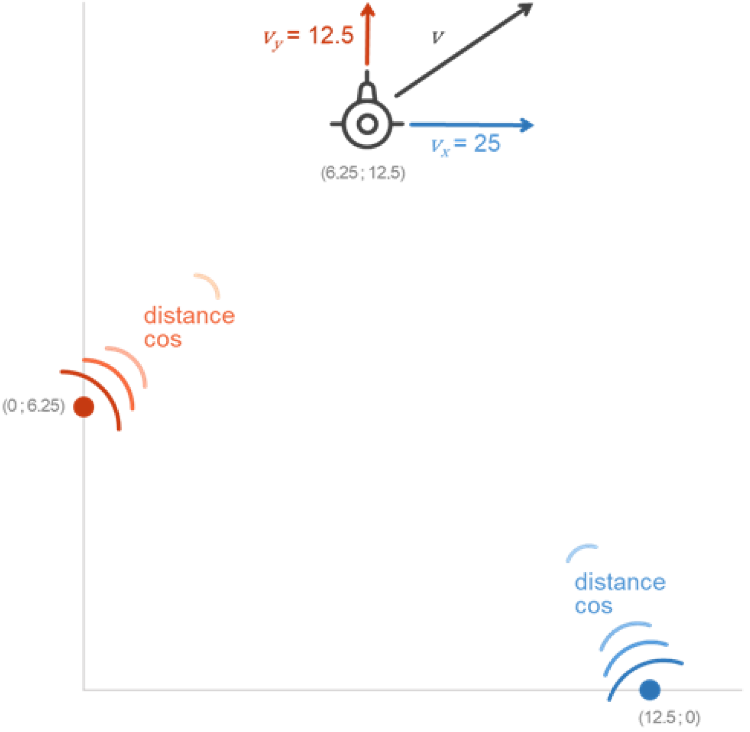
It is assumed that the AUV moves at a depth in the horizontal plane $Oxy$. Random noise is added to the current speed at each moment, simulating chaotic maneuvering. The coordinates of the AUV trajectory are denoted, as is customary, as $x\left(t\right)$ and $y\left(t\right).$ Note that these designations should be distinct from the designations of the state vector $x_t$ and observations $y_t$ in the original models (1), (2), or (3). The unit of position measurements is in kilometers (km), time is in hours (h), and speeds are measured in km/h. The continuous movement model is sampled in increments of $\delta =0.0001$ h, corresponding to a frequency of about three measurements per second. For the convenience of a graphical representation of the results, it is assumed that the movement begins at time $t=0$ and ends at time $t=1000$, i.e., the movement lasts 6 min. The systematic constant AUV speed values are $v_x=25$ km/h and $v_y=12.5$. During the movement, the AUV moves an average of $3$ km. The Gaussian vector gives the initial position of the AUV ${\left(x\left(0\right),y\left(0\right)\right)}^{\prime }$, which has the mean ${\left(6.25;12.5\right)}^{\prime }$ and the covariance $\mathrm{d}\mathrm{i}\mathrm{a}\mathrm{g}\left\{{2.5}^2;5^2\right\}.$

The same type of observers are located at two points on the same $Oxy$ plane: the first has coordinates $\left(0,l_y\right)$, $l_y=6.25,$ i.e., it is located $6.25$ km from the origin on the $Oy$ axis, the coordinates of the second are $\left(l_x,0\right)$, $l_x=12.5,$ i.e., $12.5$ km from the origin on the $Ox$ axis. Assuming that acoustic sonars are used for observation and that the speed of sound in water is equal to $v_s=5400$ km/h, it is possible to determine the maximum possible delay of observations $T=50$, i.e., the maximum value by which observations can be delayed is $18$ s. Accordingly, the filtering process and the first estimate appear at time $T$, i.e., $18$ s after the start of movement (we can assume after the target is detected).

The source of the observer model is typical acoustic sonars [45,46] that measure the bearing and Doppler frequency shift. So, we can assume that the azimuth angle and range are measured, i.e., the AUV acoustic signature is considered known. Each observer measures the range and the direction cosine to the target with an additive measurement error. The error vector is assumed to be the Gaussian with mean ${\left(0,0,0,0\right)}^{\prime }$ and the covariance $\mathrm{d}\mathrm{i}\mathrm{a}\mathrm{g}\left\{{0.001}^2,{0.005}^2,{0.001}^2,{0.005}^2\right\}.$ One can use the work [47] to understand the accuracy parameters of real devices. The scheme of movement and observation is illustrated in Figure 1.

So, we have the following observation system. The state vector has the form

$$\begin{array}{c}x\left(t\right)=x\left(t-1\right)+\delta v_x+w_x\left(t\right),\\ y\left(t\right)=y\left(t-1\right)+\delta v_y+w_y\left(t\right).\end{array}$$

(12)

Describing chaotic velocity changes vector ${\left(w_x\left(t\right),w_y\left(t\right)\right)}^{\prime }$ is assumed to be Gaussian with mean ${\left(0,0\right)}^{\prime }$ and two variants of covariances: (1) $\mathrm{d}\mathrm{i}\mathrm{a}\mathrm{g}\left\{{0.0025}^2;{0.0025}^2\right\}$ and (2) $\mathrm{d}\mathrm{i}\mathrm{a}\mathrm{g}\left\{{0.01}^2;{0.01}^2\right\}$. Accordingly, in the first case, the AUV can change the speed by about 25 km/h, and in the second, by about $100$ km/h. Thus, case (2) is about a high-speed maneuvering target. For the presented calculation, it is more interesting because it gives a very diverse trajectory.

The measurements performed are denoted by $d_1\left(t\right), d_2\left(t\right)$ (distances measured by the first and second observers) and $c_1\left(t\right), c_2\left(t\right)$ (direction cosines measured by the first and second observer). The vector of observation errors is denoted by ${\left(v_{d_1}\left(t\right),v_{d_2}\left(t\right),v_{c_1}\left(t\right),v_{c_2}\left(t\right)\right)}^{\prime }$. Thus, the observation vector is as follows:

$$\begin{array}{l}{d}_1\left(t\right)=\sqrt{{\left(x\left(t-{\left({\tau }_t\right)}_1\right)\right)}^2+{\left(y\left(t-{\left({\tau }_t\right)}_1\right)-l_y\right)}^2}+v_{d_1}\left(t\right),\\ c_1\left(t\right)=\frac{\left(y\left(t-{\left({\tau }_t\right)}_1\right)-l_y\right)}{\sqrt{{\left(x\left(t-{\left({\tau }_t\right)}_1\right)\right)}^2+{\left(y\left(t-{\left({\tau }_t\right)}_1\right)-l_y\right)}^2}}+v_{c_1}\left(t\right),\\ d_2\left(t\right)=\sqrt{{\left(x\left(t-{\left({\tau }_t\right)}_2\right)-l_x\right)}^2+{\left(y\left(t-{\left({\tau }_t\right)}_2\right)\right)}^2}+v_{d_1}\left(t\right),\\ c_2\left(t\right)=\frac{\left(x\left(t-{\left({\tau }_t\right)}_2\right)-l_x\right)}{\sqrt{{\left(x\left(t-{\left({\tau }_t\right)}_2\right)-l_x\right)}^2+{\left(y\left(t-{\left({\tau }_t\right)}_2\right)\right)}^2}}+v_{c_2}\left(t\right).\end{array}$$

(13)

Taking into account the selected sampling step $\delta$ and the speed of sound in water $v_s$, the values ${\left({\tau }_t\right)}_1$ and ${\left({\tau }_t\right)}_2$ are expressed in terms of the observer distances up to the AUV, i.e.,

$$\begin{array}{c}{\left({\tau }_t\right)}_1=\mathrm{m}\mathrm{i}\mathrm{n}\left\{T,\left[\sqrt{{\left(x\left(t\right)\right)}^2+{\left(y\left(t\right)-l_y\right)}^2}/\left({\delta v}_s\right)\right]\right\},\\ {\left({\tau }_t\right)}_2=\mathrm{m}\mathrm{i}\mathrm{n}\left\{T,\left[\sqrt{{\left(x\left(t\right)-l_x\right)}^2+{\left(y\left(t\right)\right)}^2}/\left({\delta v}_s\right)\right]\right\}.\end{array}$$

(14)

In (14), the notation $\left[x\right]$ is used for the floor function of $x$, and the potential possibility of removing an observed object at a distance for which the delay value becomes greater than the specified maximum $T$ is taken into account.

4.2. CMNF Structure

To implement the CMNF algorithm, it is required to determine the structure of the filter, i.e., to select the basic prediction function ${\xi }_t={\xi }_t\left(x\right)$ and the basic correction function ${\zeta }_t={\zeta }_t\left(x,y\right)$. The linear model of movement (12) does not require clarification of the typical choice of the structure due to the system, i.e.,

$${\xi }_t\left({\widehat{x}}_{t-1}\right)={\phi }_t\left({\widehat{x}}_{t-1},\mathrm{E}\left\{w_t\right\}\right)=\left(\begin{array}{c}\widehat{x}\left(t-1\right)+\delta v_x\\ \widehat{y}\left(t-1\right)+\delta v_y\end{array}\right).$$

We can also try and choose a residual as the basic correction structure, i.e.,

$${\zeta }_t\left({\tilde{x}}_t,y_t\right)=y_t-{\psi }_t\left({\tilde{x}}_t,\mathrm{E}\left\{v_t\right\}\right)=\left(\begin{array}{l}\begin{array}{l}{d}_1\left(t\right)-\sqrt{{\left(\tilde{x}\left(t\right)\right)}^2+{\left(\tilde{y}\left(t\right)-l_y\right)}^2}\end{array}\\ \begin{array}{l}\begin{array}{c}\begin{array}{l}{c}_1\left(t\right)-\frac{\left(\tilde{y}\left(t\right)-l_y\right)}{\sqrt{{\left(\tilde{x}\left(t\right)\right)}^2+{\left(\tilde{y}\left(t\right)-l_y\right)}^2}}\end{array}\\ \begin{array}{l}{d}_2\left(t\right)-\sqrt{{\left(\tilde{x}\left(t\right)-l_x\right)}^2+{\left(\tilde{y}\left(t\right)\right)}^2}\end{array}\end{array}\\ c_2\left(t\right)-\frac{\left(\tilde{x}\left(t\right)-l_x\right)}{\sqrt{{\left(\tilde{x}\left(t\right)-l_x\right)}^2+{\left(\tilde{y}\left(t\right)\right)}^2}}\end{array}\end{array}\right).$$

(15)

In theory, even the fact that the delay ${\tau }_t$ is not taken into account in the residual (15) should not interfere with the operation of the filter. However, the first experiments have already shown that the structure (15), although it gives a working filter, could have a higher accuracy. The apparent idea is to supplement (15) with a delay estimate of the form (14), i.e.,

$$\begin{array}{c}\begin{array}{c}{\left({\tilde{\tau }}_t\right)}_1=\sqrt{{\left(\tilde{x}\left(t\right)\right)}^2+{\left(\tilde{y}\left(t\right)-l_y\right)}^2}/\left({\delta v}_s\right),\end{array}\\ {\left({\tilde{\tau }}_t\right)}_2=\sqrt{{\left(\tilde{x}\left(t\right)-l_x\right)}^2+{\left(\tilde{y}\left(t\right)\right)}^2}/\left({\delta v}_s\right),\end{array}$$

(16)

but two different delays did not lead to an improvement in the result.

A positive result was obtained when the observations’ physical nature was considered in the correction structure. Namely, if we assume that there is no noise in (13), we can determine the AUV’s position by recalculating the distances and cosines into Cartesian coordinates. Such a transformation gives the following correction structure:

$${\zeta }_t\left({\tilde{x}}_t,y_t\right)=\left(\begin{array}{c}\sqrt{{\left(d_1\left(t\right)\right)}^2-{\left(c_1\left(t\right)d_1\left(t\right)\right)}^2}+{\left({\tilde{\tau }}_t\right)}_1{v}_x\\ \begin{array}{c}\begin{array}{c}{c}_1\left(t\right)d_1\left(t\right)+l_y+{\left({\tilde{\tau }}_t\right)}_1{v}_y\\ c_2\left(t\right)d_2\left(t\right)+l_x+{\left({\tilde{\tau }}_t\right)}_2{v}_x\end{array}\\ \sqrt{{\left(d_2\left(t\right)\right)}^2-{\left(c_2\left(t\right)d_2\left(t\right)\right)}^2}+{\left({\tilde{\tau }}_t\right)}_2{v}_y\end{array}\end{array}\right).$$

(17)

In addition to the geometry of observations in correction (17), the delay estimate (16) is also used. Thus, (17) are two estimates of the AUV position that each observer could give independently without considering measurement errors. Combining these estimates and taking into account the impact of errors is already the filter’s task, i.e., of the relations (10).

It should be noted that the demonstrated flexibility in selecting the estimate structure is the key advantage of the CMNF.

4.3. Computer Simulations

In each of the performed computer computations, we simulated two independent beams of $\mathrm{100,000}$ trajectories of the observation system (12)–(14) and CMNF estimates (9). On the first beam, the filter parameters were calculated according to the formulas in (10) and their accuracy according to Formula (11). Accordingly, the statistical average replaced mathematical expectations according to the Monte Carlo method. On the second beam, the actual quality of the CMNF estimate ${\widehat{x}}_t{=\left(\widehat{x}\left(t\right),\widehat{y}\left(t\right)\right)}^{\prime }$ was evaluated. The mean square deviations of the estimate errors determine the estimation accuracy of the coordinates of the AUV position. These values, denoted by ${\sigma }_{\widehat{x}}\left(t\right),{\sigma }_{\widehat{y}}\left(t\right)$, were calculated from the second beam of trajectories, and can be called practical accuracy.

The values $\sqrt{{\left({\widehat{K}}_t\right)}_{\mathrm{1,1}}}$ and $\sqrt{{\left({\widehat{K}}_t\right)}_{\mathrm{2,2}}}$ represent the theoretical accuracy of the CMNF estimate. We calculated these values using Formula (11) and compared them with ${\sigma }_{\widehat{x}}\left(t\right)$ and ${\sigma }_{\widehat{y}}\left(t\right),$ respectively.

Calculations were performed for two variants of maneuvering speed (let us call them, conditionally, a maneuver of $25$ km/h and a maneuver of $100$ km/h) and two correction options: the main (17) and the residual (15). For a qualitative assessment of the results, each of the calculations was repeated under the assumption that $T=0$, i.e., in a model that does not consider the observation delays. The following series of figures illustrate the results.

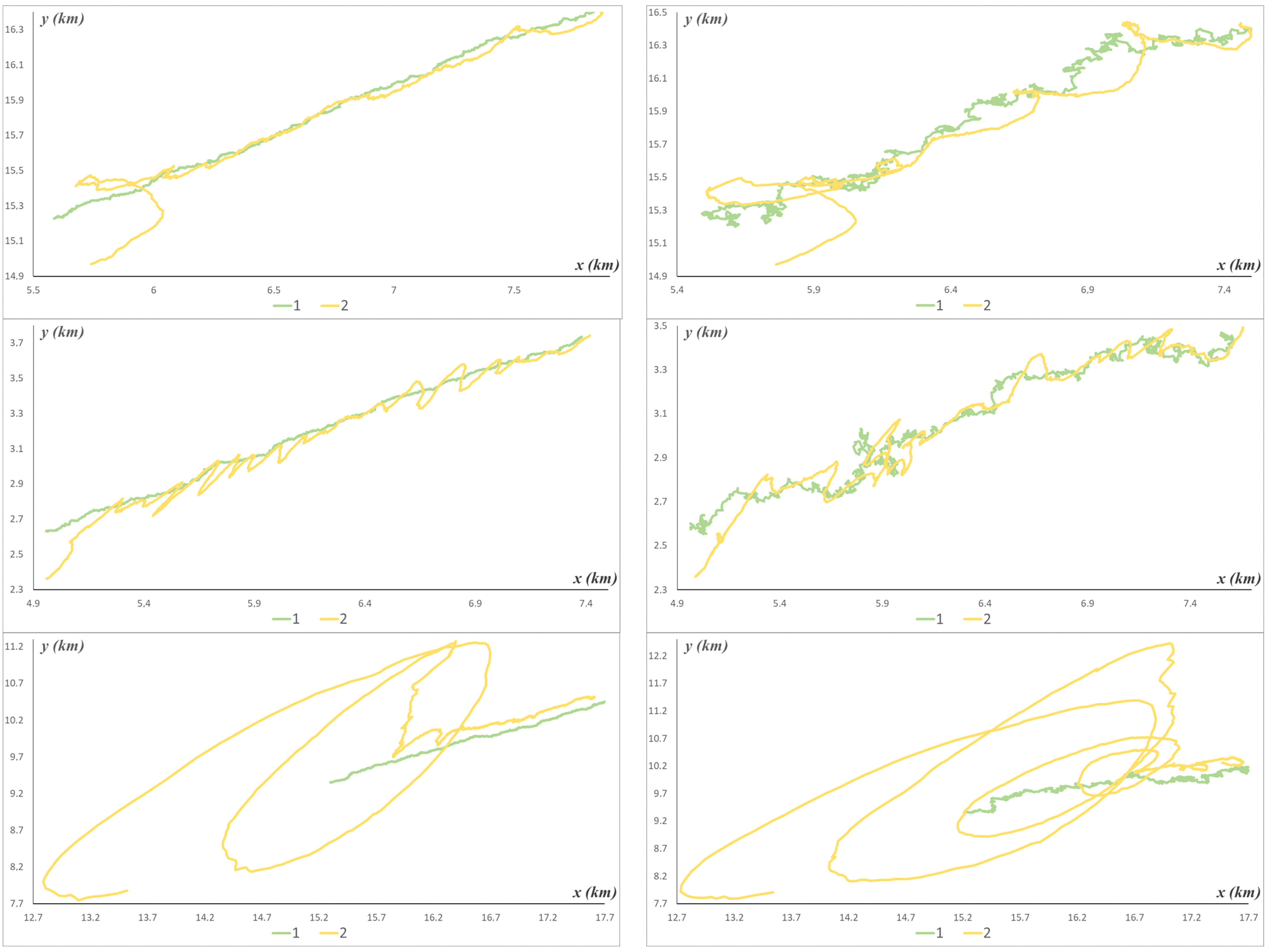
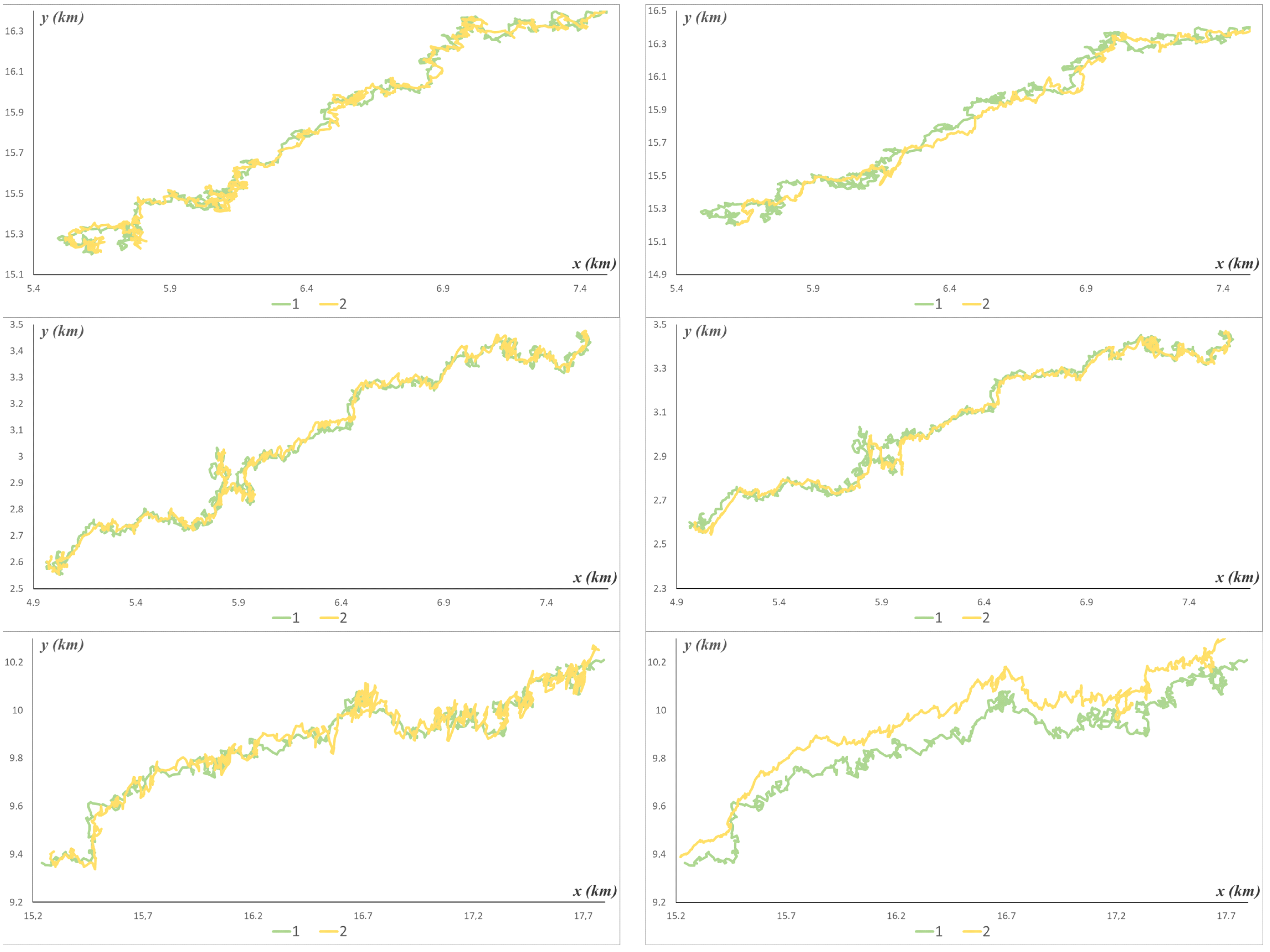
Figure 2 shows several AUV trajectories ${\left(x\left(t\right),y\left(t\right)\right)}^{\prime }$ for a maneuver of $25$ km/h (left) and a maneuver of $100$ km/h (right), and the corresponding CMNF estimates ${\left(\widehat{x}\left(t\right),\widehat{y}\left(t\right)\right)}^{\prime }$ calculated using correction (17). This figure and the following ones show the same trajectories from the simulated beam, i.e., the same set of random variables forms the states and estimates, and the difference is only in the value of the model parameters (in Figure 2, these parameters are variances of $w_x\left(t\right)$ and $w_y\left(t\right)$). This figure gives a qualitative idea of the filtering results and explains why the trajectories for a maneuver of $100$ km/h are more interesting to study.

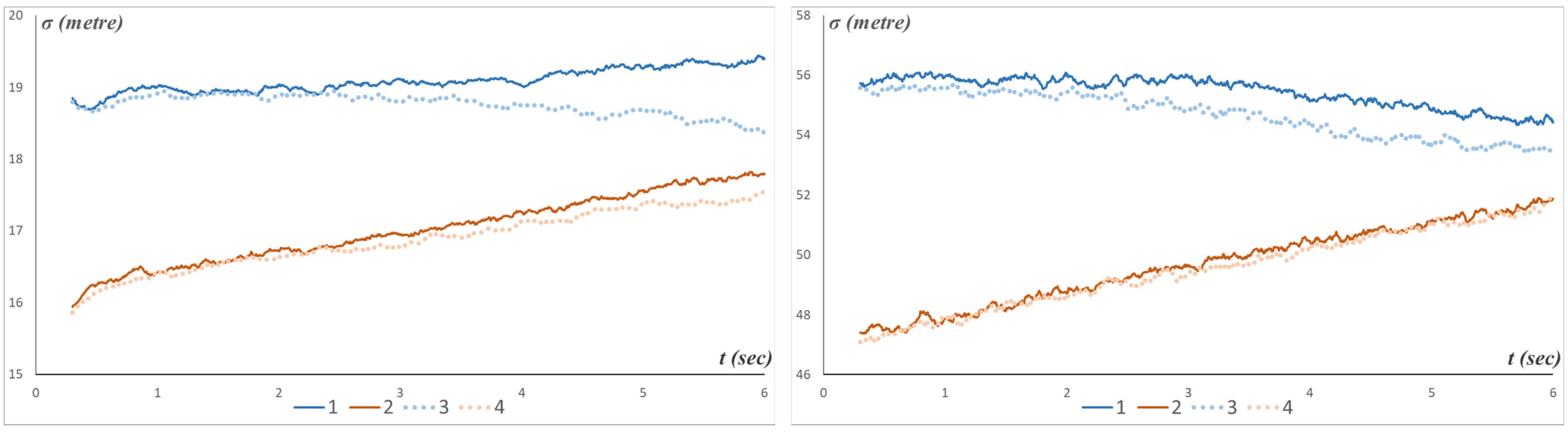
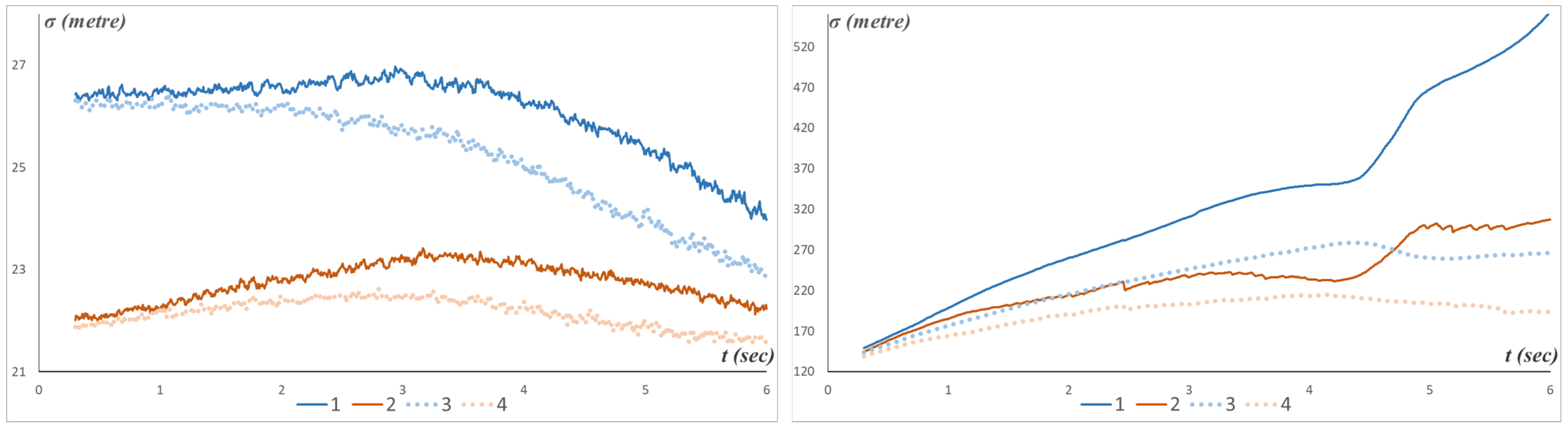
A formal analysis of filtering quality is presented in Figure 3. This figure gives quantitative estimates of the effectiveness of target tracking, shows the extent of deterioration in the quality of estimates between a maneuver of $25$ km/h and a maneuver of $100$ km/h, and also confirms the applicability of the Monte Carlo method for the practical synthesis (training) of CMNF, since the theoretical and practical accuracy are very close.

The same illustrations, as shown in Figure 2 and Figure 3, are repeated in the following Figure 4 and Figure 5 with a single change: instead of correction (17), we use the correction (15). These figures support the above statement about the correction in the form of a residual that is not very suitable for the model under consideration. Not only did the filtering quality turn out to be very low, but the difference between the theoretical and practical accuracy of the CMNF is also unacceptably large. The latter circumstance can be dealt with by increasing the size of the training beam used for approximate calculations using Formula (10), but it is impossible to improve the quality compared to the theoretical ones $\sqrt{{\left({\widehat{K}}_t\right)}_{\mathrm{1,1}}}$ and $\sqrt{{\left({\widehat{K}}_t\right)}_{\mathrm{2,2}}}$ in any case.

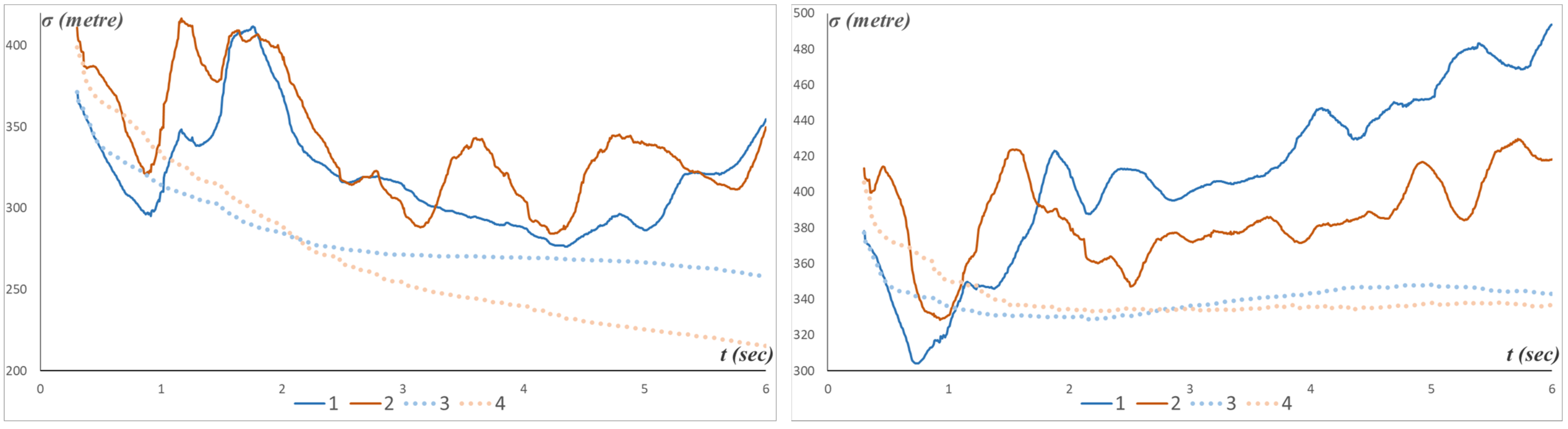
The last group of figures is given in order to illustrate the influence of the main factor of the model proposed here: the delay of observations ${\tau }_t$. We should immediately note that it is not advisable to consider figures of both variants of the maneuver, so for graphical presentations, we have limited ourselves to only the maneuver of $100$ km/h, as it is more beautiful. Accordingly, the same trajectories and the exact figures above are given to compare corrections (15) and (17). Figure 6 shows the trajectories, and Figure 7 illustrates the filtering accuracy.

These visual and quantitative figures illustrate the real difference between models with and without observation delays. Nevertheless, they also show that the quality of a universal filter with a simple correction that needs to consider the specifics of the movement observation model needs to be higher. Of course, as seen in Figure 7 on the right, the difference between the theoretical and practical accuracy of the CMNF estimates will disappear as the size of the training beam increases. However, the absolute advantage of the “smart” correction will remain.

Finally, the calculations’ results are presented in tabular form. Namely,

Table 1. Average indicators of filtering accuracy.

Model with Delays
Basic correction function ${\zeta }_t\left({\tilde{x}}_t,y_t\right)$
«Geometric correction» (17)				«Residual» (15)
Real accuracy		Theoretical accuracy		Real accuracy		Theoretical accuracy
$\widehat{\mathrm{E}}\left\{{\sigma }_{\widehat{x}}\left(t\right)\right\}$	$\widehat{\mathrm{E}}\left\{{\sigma }_{\widehat{y}}\left(t\right)\right\}$	$\widehat{\mathrm{E}}\left\{\sqrt{{\left({\widehat{K}}_t\right)}_{\mathrm{1,1}}}\right\}$	$\widehat{\mathrm{E}}\left\{\sqrt{{\left({\widehat{K}}_t\right)}_{\mathrm{2,2}}}\right\}$	$\widehat{\mathrm{E}}\left\{{\sigma }_{\widehat{x}}\left(t\right)\right\}$	$\widehat{\mathrm{E}}\left\{{\sigma }_{\widehat{y}}\left(t\right)\right\}$	$\widehat{\mathrm{E}}\left\{\sqrt{{\left({\widehat{K}}_t\right)}_{\mathrm{1,1}}}\right\}$	$\widehat{\mathrm{E}}\left\{\sqrt{{\left({\widehat{K}}_t\right)}_{\mathrm{2,2}}}\right\}$
Maneuver ${\mathit{w}}_{\mathit{x}}\left(\mathit{t}\right)$, ${\mathit{w}}_{\mathit{y}}\left(\mathit{t}\right)~25$ km/h
21.76	22.06	21.45	21.90	329.26	352.23	293.69	283.14
Maneuver ${\mathit{w}}_{\mathit{x}}\left(\mathit{t}\right)$, ${\mathit{w}}_{\mathit{y}}\left(\mathit{t}\right)~100$ km/h
57.61	54.31	56.88	54.13	414.72	394.69	348.55	352.25
Model without delays
Maneuver ${\mathit{w}}_{\mathit{x}}\left(\mathit{t}\right)$, ${\mathit{w}}_{\mathit{y}}\left(\mathit{t}\right)~25$ km/h
16,73	17,37	16,24	16,98	212,93	146,11	139,75	119,33
Maneuver ${\mathit{w}}_{\mathit{x}}\left(\mathit{t}\right)$, ${\mathit{w}}_{\mathit{y}}\left(\mathit{t}\right)~100$ km/h
28.72	27.76	27.88	27.16	321.76	235.99	232.61	196.23

shows the average values of the quality indicators for all sets of parameters. The average value is understood as averaging over time, for example $\widehat{\mathrm{E}}\left\{{\sigma }_{\widehat{x}}\left(t\right)\right\}=\frac{1}{T}\sum _{t=1}^T{\sigma }_{\widehat{x}}\left(t\right)$, etc.

5. Conclusions

Summing up the article, we repeat the main provisions:

• In target tracking tasks where acoustic sonars are used, it is necessary to take into account the random delay of observations according to model (1) or its simplified versions, (2) and (3);
• The optimal solution of the tracking problem for the simplest model, (3), described by a Bayesian filter, can be written out but cannot be implemented practically;
• The method of conditionally minimax nonlinear filtering can be applied to a model with random observation delays;
• In problems with observers of the “geometric” type, the use of simple universal filters can lead to unsatisfactory results even in simple observation conditions; taking into account the physical nature of observations can dramatically improve the quality of filtering.

The presented relatively complete picture of the model with random delays of indirect observations and the problem of filtering its state includes a theoretical description of the model and the optimal Bayesian filter, a practically consistent algorithm of conditionally nonlinear minimax filtering, an applied experiment with a model of AUV movement close to practice and observations of it with typical sonars. At the same time, the following question remains open. Many parameters used in the experimental model can indeed be known or established experimentally. But part of the parameters, and above all, the systematic component of the AUV velocity $v_t={\left(v_x,v_y\right)}^{\prime }$, cannot be known in advance. Thus, the possibility of identifying these parameters in parallel with goal tracking comes to the forefront. In addition, the constancy of speed also does not look like a realistic assumption. So, for practical purposes, we need to learn how to identify the speed in a reasonably short observation period and repeat the identification process as necessary. Further research is supposed to be devoted to this issue.