Formation Tracking Control for Multi-Agent Systems with Collision Avoidance and Connectivity Maintenance

Abstract

This paper investigates the formation tracking control of multiple agents with a double-integrator model and presents a novel distributed control framework composed of three items: a potential-based gradient term, a formation term, and a navigation term. Considering the practical situation, each agent is regarded as a rigid-body with a safe radius and a sensing region. To enable collision avoidance and connectivity maintenance among multiple agents, a new potential function with fewer parameters is established. The predetermined formation is also achieved by taking the difference between the actual displacement and the desired displacement as a consensus variable. Lastly, the virtual navigator provides trajectory signals and guides the multiple agent movement. Two instances of an equilateral triangle formation and a hexagonal formation are used in the simulation to verify the proposed method.

1. Introduction

Numerous advances and discoveries in the study of natural biological community behavior [1] (e.g., migrating of birds, schools of fish, and swarms of ant colonies) have brought new inspiration for a multi-agent coordinated control methodology in recent decades, which has attracted the focus of many scholars [2,3]. Formation control is one of the most basic and crucial concerns of cooperative control, which has been widely applied in practical engineering projects; e.g., the formation of Multi-robot systems [4], the formation of Unmanned Aerial Vehicles (UAVs) [5,6,7], and the formation of Multiple Autonomous Underwater Vehicles (AUVs) [8].

According to the type of control variables, formation control can be classified into position-based control [9], distance-based control [10,11,12], bearing-based control [13,14,15], and displacement-based control [16,17,18]. Among them, the sensing and control variables of position-based formation control are the positions of each agent in a global coordinate system, which necessitates more sophisticated sensing capabilities. In contrast, distance-based formation control only requires measuring the inter-agent distances in the neighbors of each agent, which reduces the need for complex sensing capabilities, and thus, is widely used in practice. However, the application of this method hinges on strong interactivity. Bearing-based formation control, like distance-based formation control, has received increasing attention due to its minimal demands on the sensing ability of each agent. However, most of the previous studies have been limited to planar formations and have focused on controlling the subtended bearing angles, which are measured in the local coordinate of each agent. In the displacement-based approach, each agent must utilize its own onboard sensors to measure the relative states (positions and velocities) of its neighbors with respect to a local coordinate system, which should be aligned with the global coordinate system. Moreover, this approach requires less sensing and interaction capabilities than the other formation control methods mentioned above. A comprehensive survey on formation control can be found in [19].

Multi-agent collision avoidance is an essential and non-negligible issue in distributed formation control, and it imposes strict safety requirements on the real-time distance between agents. The artificial potential field (APF) method has the advantage of a simple architecture to avoid collisions in real time, and thus, is one of the most extensive options in collision avoidance research. In [20], Khatib initially proposed a unique real-time obstacle avoidance approach for manipulators and mobile robots based on APF. Later, fruitful works on APF for multi-agent systems emerged [21,22,23,24,25,26,27,28,29,30,31]. In [21], the collective potential function makes the relative position of any two agents in the group converge to a given distance. In [22], the authors extended this method to design a formation tracking controller by incorporating a smooth and p-time differential bump function into the potential function. In [23], a formation control strategy was developed that implements an artificial potential field to avoid collisions for a class of second-order nonlinear multi-agent systems. In [24], the relative distance constraints between arbitrary adjacent agents can be ensured by the artificial potential function. In addition, the idea of the potential function was drawn in [26] and implemented as an explicit expression for flocking control to make sure that no collisions occur between the mobile agents in [25]. In [27,28], the authors adopted various potential functions to enable both connectivity preservation and obstacle avoidance between multiple agents at the same time. Furthermore, artificial potential fields were applied in engineering to assist with collision avoidance. An effective improved artificial potential function (IAPF)-based path planning approach was presented for the multi-UAV systems in [29]. For the collision and obstacle avoidance problems in the formation process, the artificial potential field was used as the multi-autonomous underwater vehicles system formation planning design [30]. However, the aforementioned APF for multi-agent collision avoidance has several limitations. First, the approaches designed in [22,23,25,29], will lead to the infinite potential force when the distance between two agents is close to 0. This hinders their adoption in many real-life applications. Second, the control protocols [27] are only applied to single-integrator systems, which, cannot capture dynamics features for a wide range of systems. Third, many important design parameters related to action function need to be considered in APF [21]. Fourth, some artificial potential function models, such as those proposed in [24,28], are complicated in terms of construction process. Last, given the fact that the agents in the context of formation control are usually defined by practical robots/UAVs/USVs with non-negligible shape [22,29,30], it may be unsuited to model the agent as a particle [21,24,25,26], since doing so ignores the probability of collision between agents. Considering the agent as a rigid-body with a safe radius is an appropriate method [23,27,28].

Multi-agent interaction is also of fundamental importance in formation control. Existing work can be categorized into fixed network topology [32,33,34,35,36] and time-varying network topology [37,38]. A mathematical model for an M-dimensional asynchronous swarm with a fixed communication topology was constructed [32]. In [32], the authors presented a multi-layer formation control scheme that is limited to the fixed topology. In [34], the author developed a quadratic leader-following consensus protocol for multi-quadrotor aircraft subject to the fixed topology. Similarly, a fixed-time control protocol implementing directed fixed topology was studied in [35], in which six agents keep a periodic time-varying regular hexagonal formation. Moreover, the fault-tolerant formation control problem for heterogeneous vehicles was addressed for communication link faults and actuator faults under the connection of the fixed topology network [36]. However, it is required that the fixed network should be connected all the time, which is usually difficult to achieve in practice. By comparison, designing the time-varying network for formation control is more feasible given the limited sensing ability of each agent. In [37], the author studied the time-varying formation tracking problems for second-order multi-agent systems with switching interaction topologies. The work [38] implemented a barycentric coordinate to deal with the formation control problem under directed and switching sensing topologies. It is worth pointing out that the interaction power of the multi-agent system is determined by its limited sensing radius, and the topology network is disconnected when the distance between agents is beyond the sensing radius. As a result, the work of maintaining connectivity is necessary [39,40,41,42,43,44,45,46,47]. Using the Laplacian matrix of a graph and the properties of its spectrum, the authors in [39] viewed connectivity as a virtual barrier in space that could be overcome with artificial fields. In [40], the authors introduced the connectivity constraint function to maintain the connectivity between robots, but did not consider the collision problem between robots. In [41], the authors considered the communication range and collision avoidance range for nonholonomic mobile robots and designed dynamic surfaces based on nonlinear transformation errors to achieve connectivity preservation and collision avoidance, but the method relies on the entity leaders, which, if it malfunctions, can cause the formation to collapse. A control barrier function method that is also related to the entity leader was considered to achieve both collision avoidance and connectivity maintenance [42]. For the connectedness of the network to be maintained, the authors in [43,44] selected an appropriate potential function, respectively, to ensure multi-agent flocking and rendezvous, but did not design the body radius for multi-agent systems. In [45,46], although connectivity preservation issues were taken into account, the communication topology graph is all fixed. A navigation control for maintaining connectivity and avoiding collisions between a general class of second-order uncertain nonlinear multi-agent systems in a bounded workspace was presented in [47], in which each agent knows all signals of its neighboring agents, including positions, Euler angles, and velocities, which pose great challenges for onboard facilities. While a lot of attention has been focused on multi-agent system connection maintenance research, there are many limitations, as mentioned above in [40,41,42,43,44,45,46,47], and the scenario where the agent model has a sensing range and a body radius has received less attention [27,28,46,47].

Inspired by the above discussion, this paper proposes a novel formation control scheme for a multi-agent with a linear double-integrator model. We regard each agent as a rigid-body with a safe radius and a sensing radius, and construct a simple potential function with few parameters to fulfill the objectives of collision avoidance and connectivity maintenance among multiple rigid agents. The formation is based on the error between the actual relative positions and the expected relative positions. Furthermore, we design reference signals for the multi-agent system to make them track the desired motion trajectory. In comparison with existing work in the literature, the highlights of this paper are discussed as follows:

(1)

Collision avoidance and connectivity maintenance of multi-agent systems are essential components. In [28,45], potential functions for these two issues were separately established to deal with them, but, in this paper, the above two problems are handled together by one potential function. In addition, compared to [27,28,43], the potential function designed in this paper has fewer parameters and a simpler structure.

(2)

In [28], the adjacency weights of any two agents switched from 0 to 1 when they built up contact, and this caused the adjacency matrix and Laplacian matrix to be discontinuous. Furthermore, in [28,42,46], the adjacency weight for any two agents could not represent the fact that the power of the interconnection was restricted by distance. As a result, we employ a bump function and incorporate it into the adjacent matrix that smoothly varies from 0 to 1 to address the two problems.

(3)

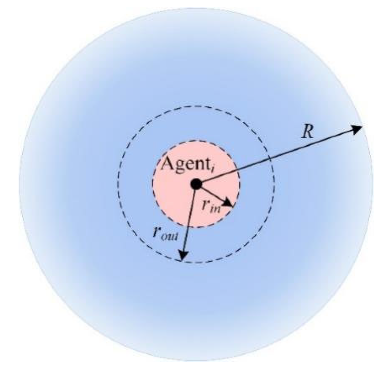
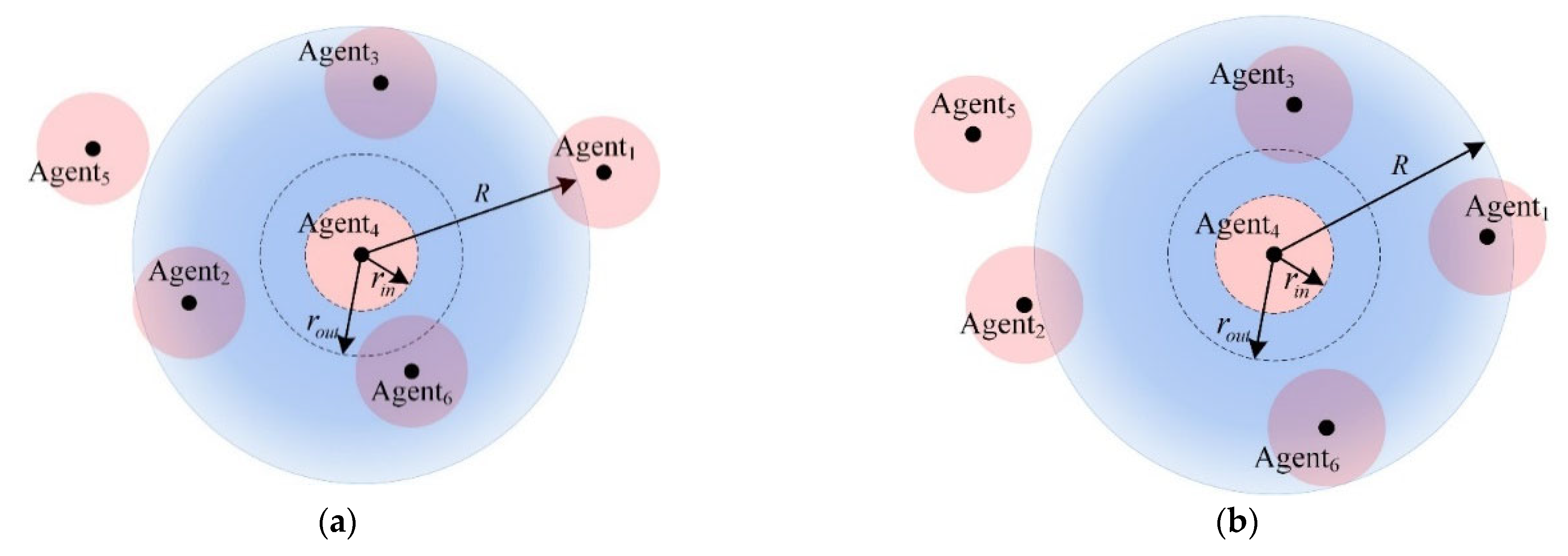
In [23], the author designed collision avoidance areas and collision areas for multi-agent systems. In addition, the collision region and communication region were also considered in [41,45,46,47]. However, these works were all associated with fixed communication topologies that have disadvantages in practice. In this paper, we transform the fixed communication topology into the time-varying topology by designing the sensing radius to overcome the disadvantage.

The remainder of this paper is organized as follows. In Section 2, problem formulation is discussed. After introducing the distributed formation control algorithm in Section 3, we also perform the stability analysis. In Section 4, the simulation demonstrates the presented control protocol. Section 5 concludes this article.

2. Problem Formulation

2.1. Agent Model

Consider a multi-agent system composed of n agents in an m-dimensional space ℝ^m. All agents are viewed as a particle with a double-integral model in general and the dynamics of agent i is as follows:

$$\begin{array}{l}{\dot{x}}_i\left(t\right)=v_i\left(t\right)\\ {\dot{v}}_i\left(t\right)=u_i\left(t\right)\end{array}$$

(1)

where x_i (t), v_i (t), u_i (t) ∈ ℝ^m are the position, velocity, and the control input of the i-th agent at time t, respectively. Let $x\left(t\right)={\left[x_1^{\mathrm{T}}\left(t\right), \cdots {, x}_n^{\mathrm{T}}\left(t\right)\right]}^{\mathrm{T}}$, $v\left(t\right)={\left[v_1^{\mathrm{T}}\left(t\right), \cdots {, v}_n^{\mathrm{T}}\left(t\right)\right]}^{\mathrm{T}}$ and $u\left(t\right)={\left[u_1^{\mathrm{T}}\left(t\right), \cdots {, u}_n^{\mathrm{T}}\left(t\right)\right]}^{\mathrm{T}}$ be the mn × 1 vector resulting from stacking the coordinates of the agents into a single vector.

In addition, consider the virtual navigator dynamics:

$$\begin{array}{l}{\dot{x}}_r\left(t\right)=v_r\left(t\right)\\ {\dot{v}}_r\left(t\right)=f_r\left(x_r,v_r,t\right)\end{array}$$

(2)

where x_r (t) ∈ ℝ^m and v_r (t) ∈ ℝ^m are the position and velocity of the virtual navigator; x_r (t₀) and v_r (t₀) are the initial position and initial velocity at initial time t₀; and f_r (x_r, v_r, t) ∈ ℝ^m is an exogenous command. For convenience, the time variable t is omitted below.

Remark 1.

In (1), the subject of our study favors unmanned aerial vehicles (UAVs), thus we adopt the simplified UAV double-integral model in [48]. In (2), the virtual navigator either differs from the virtual leader in [23] or the cooperative entity UAV in [29], and it is to generate reference signals to plan the trajectory for multi-agents, so one can think of it as a command generator.

Remark 2.

In this article, the double-integral model will be used due to the fact that it can characterize the feature of the dynamics of multi-agent systems [28,42,43]. In fact, bounded uncertainty/disturbance should generally be considered in the agent dynamics. The proposed control strategy in this paper cannot be extended to this case by considering the negative impact generated by the bounded uncertainties or disturbances, and we intend to do this in the future.

In this paper, multi-agent systems are a homogeneous group, equipped with the same equipment and physical characteristics (e.g., sensors and size), so the agent previously regarded as a particle model cannot match the real scenario. As shown in Figure 1, the agent i has three circular areas that correspond to the three radii of r_in, r_out, and R, where r_in (0 < r_in < r_out) is the safety radius (body-radius), r_out (r_in < r_out < R) is the collision avoidance radius, and R is the sensing radius, which is preferred by the abilities of the onboard sensor.

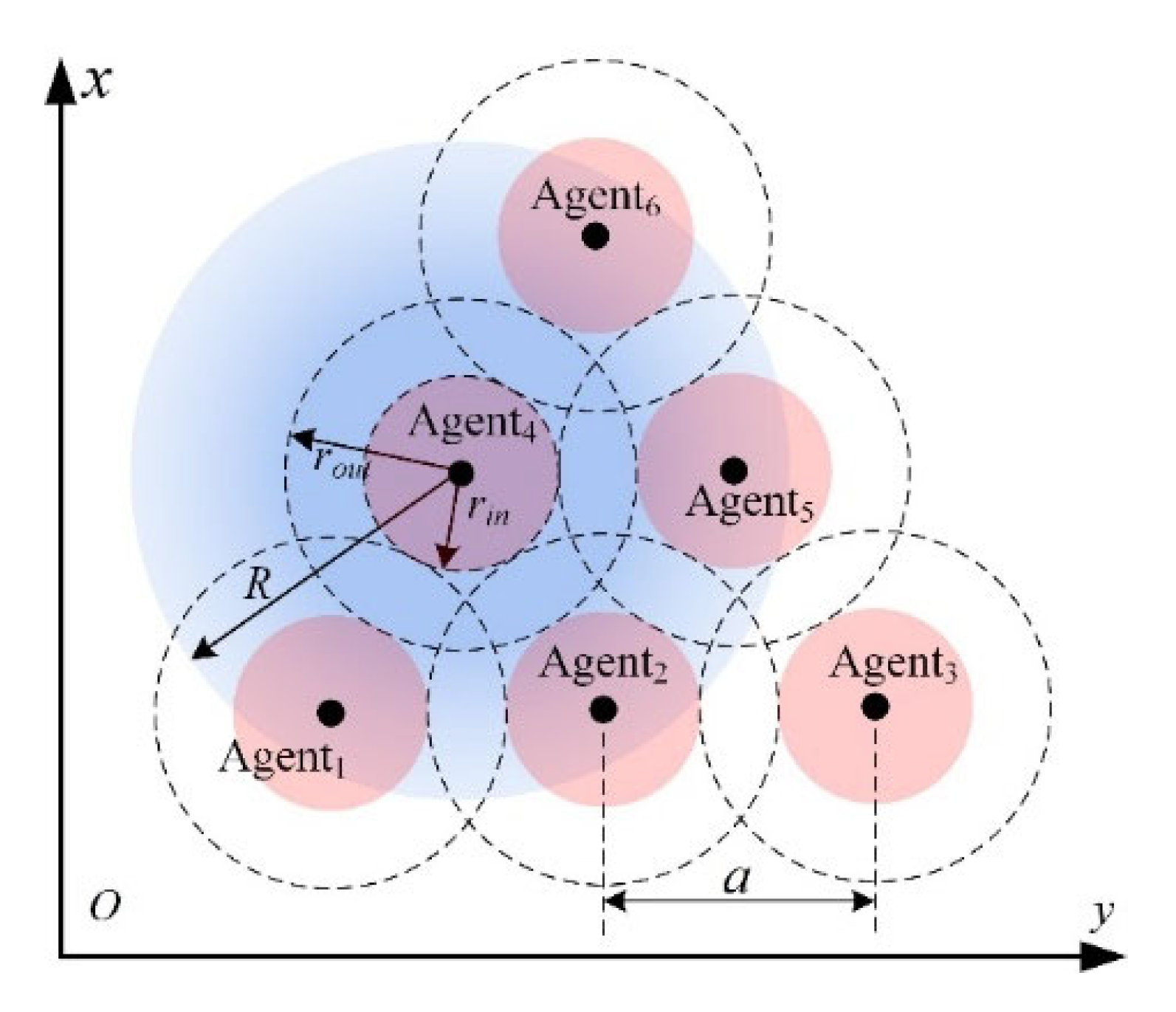
2.2. Dynamic Topology

2.2.1. Graph Theory

The interaction between agents can be represented by a graph G = (υ, ε), where υ = {1, 2, …, n} is the set of nodes that indicate the agent and ε ⊆ {(i, j): i, j ∈ υ, i ≠ j } is a list of nodes pairs (edges of the graph). If the i-th agent can obtain the information of the j-th agent, the j-th agent is said to be the neighbor of the i-th agent, and the matching weight is a_ij = 1. One defines the weighted adjacency matrix of G to be the matrix A = [a_ij] ∈ ℝ^n×n such that a_ij = 1 if (i, j) ∈ ε, and a_ij = 0 otherwise. Since self-loops are not allowed in the graph, for every i∈υ, one set a_ii = 0. Neighborhood of the agent i is defined as follows:

$$N_i=\left\{j\in \upsilon :a_{ij}\ne 0\right\}=\left\{j\in \upsilon :\left(i,j\right)\in \epsilon \right\}$$

(3)

The Laplacian L = [l_ij]∈ℝ^n×n is another crucial matrix that associated the connectivity of the graph and is defined as follows:

$$L=D-A$$

(4)

where D = diag{d₁, d₂, …, d_n}, $d_i={{\displaystyle \sum }}_{j=1}^n{a}_{ij}$ and i = 1,2, …, n.

Lemma 1.

([49]) Let λ₁≤ λ₂ ≤… ≤ λ_n be the ordered eigenvalues of the Laplacian matrix L. The graph G is then connected if and only if the following conditions are satisfied.

• λ₁ = 0, with corresponding eigenvector, i.e., the vector of all entries equal to 1;
• λ_n ≥ …λ₂ > 0.

Remark 3.

In this paper, each agent is equipped with the same onboard sensors and can be measured by each other once the agent enters the sensing radius R of other agents. Thus, the edges of the multi-agent systems are bidirectional and the Laplacian matrix is symmetric and semi-positive definite.

2.2.2. Time-Varying Graph

In contrast to the fixed topology network, in which the neighbor set is invariable, the agent with sensing radius R is continually moving in space with time, and the number and quantity of the neighbor set of each agent are changing, resulting in a time-varying graph G. Redefine the dynamic graph as follows: other agents can be observed by the agent i if they are within its radius R. Modify the neighbor set of agents i as follows, relying on the R depicted in Figure 1:

$$N_i=\left\{j\in \upsilon :d_{ij}<R\right\}$$

(5)

where${ d}_{ij}{=\Vert x}_i{-x}_j{\Vert }_m$ is the Euclidean distance in ℝ^m between agent i and j. Correspondingly, the edge set of graph G can be rewritten as:

$$\epsilon \left(x\right)=\left\{\left(i,j\right)\in \upsilon \times \upsilon :d_{ij}<R,i\ne j\right\}$$

(6)

Notice that the neighbor set and the set of edges is dependent on x. Therefore, the network of multi-agents described by (1) yields a dynamic graph G = (υ, ε(x)). The concept is demonstrated in the following example: At time t (t ≥ t₀), in a network system with six agents (see Figure 2a), agents 2, 3, and 6 are inside the detection radius R of agent 4, while agents 1 and 5 are not, so the neighbor set of agent 4 is N₄ = {2, 3, 6}, and at time t + 1, the neighborhood of agent 4 (in Figure 2b) is N₄ = {1, 3, 6} due to the movement of multi-agent.

Assumption 1.

Each agent has a local coordinate system that is aligned with the global coordinate system. Agent i can measure the relative positions x_i − x_j and the relative velocity v_i − v_j with respect to agent j by its onboard compass/IMU camera or lidar in its local coordinate system.

Remark 4.

Assumption 1 is appropriate. The local coordinate system of each agent must be aligned with the global coordinate system, which can be achieved by magnetic sensors [50]. Furthermore, the relative positions (displacements) concerning the local coordinate systems are the same as those concerning the global coordinate system, due to the alignment of the coordinate systems.

In practice, the detecting performance of the sensor is limited by the distance between it and the target, and the greater it is, the more challenging it is for the device to gain data (or the less information is obtained). So, the adjacency weight a_ij may be specified from [20] as a bump function that varies with the distances between agents i and j.

$$\zeta \left(z\right)=\left\{\begin{array}{ll}1,& z\in \left[0,h\right)\\ \left[1+\cos \left(\pi \left(z-h\right)/\left(1-h\right)\right)\right]/2,& z\in \left[h,1\right]\\ 0,& \mathrm{otherwise}\end{array}\right.$$

(7)

where h ∈ (0, 1) is a constant. Using the bump function, one can define a dynamic adjacency matrix:

$$a_{ij}=\zeta \left(d_{ij}/R\right)\in \left[0,1\right]$$

(8)

$$A(x)=\left[a_{ij}\left(x\right)\right]$$

(9)

2.3. Control Objective

Consider a group of agents modeled by the double-integrator (1) and design a distributed algorithm u_i for each agent to track the desired trajectory signal (2) while achieving and maintaining the preset formation, guaranteeing collision avoidance and connectivity maintenance at the same time. Specifically, the control goal can be mathematically expressed as:

• Track the desired trajectory: $\underset{t\to \infty }{\lim }\Vert {\nu }_{\mathrm{i}}{-\nu }_r\Vert \to 0$ (i ∈ υ), for all t ≥ t₀;
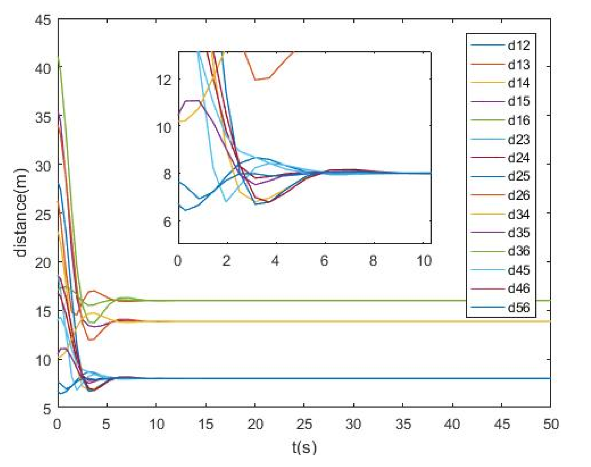
• Achieve and maintain the desired formation: $\underset{t\to \infty }{\lim }\Vert x_{ij}{-p}_{ij}^{*}\Vert \to 0$ and $\underset{t\to \infty }{\lim }\Vert {\nu }_i{-\nu }_j\Vert \to 0$ (i, j ∈ υ, i ≠ j), for all t ≥ t₀;
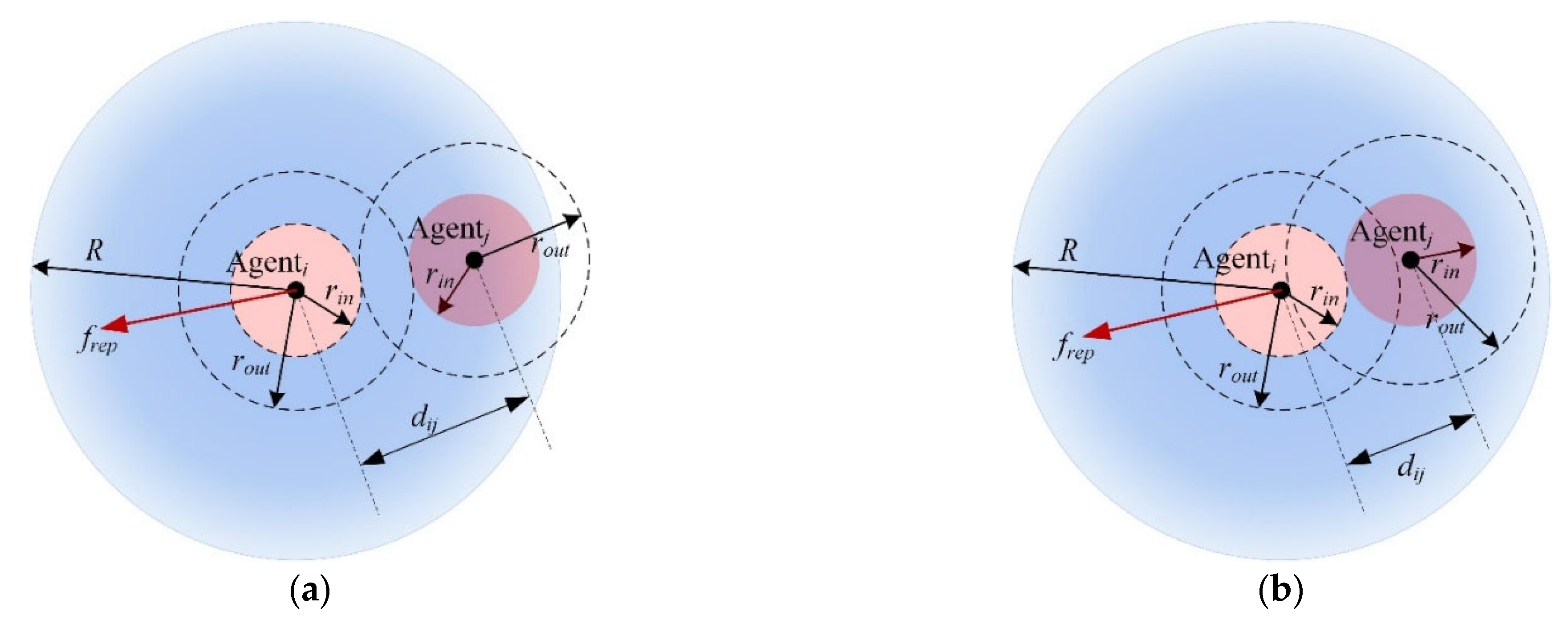
• Collision avoidance: if $d_{ij}\left(t_0\right)=\Vert x_i\left(t_0\right)-x_j\left(t_0\right)\Vert {>2r}_{in}$, then $\underset{t\to \infty }{\lim }\Vert x_i{-x}_j\Vert {>2r}_{in}$ (i, j ∈ υ, i ≠ j), for all t ≥ t₀;
• Connectivity maintenance: $\underset{t\to \infty }{\lim }\Vert x_i{-x}_j\Vert <R$ (i, j ∈ υ, i ≠ j), for all t ≥ t₀.

where x_ij and $p_{ij}^{*}$ represent the actual and desired displacement between agent i and agent j, respectively. For the sake of convenience, the following lemma is used in the proof of stability for the distributed control algorithm.

Lemma 2.

([51]) (LaSalle invariance Theorem) Let Ω ⊂ D be a compact set that is positively invariant with respect to $\dot{x}=f\left(x\right)$. Let V: D→R be a continuously differentiable function such that $\dot{V}\left(x\right)\le 0$ in Ω. Let E be the set of all points in Ω where $\dot{V}\left(x\right)=0$. Let M be the largest invariant set in E. Then every solution starting in Ω approaches M as t→∞.

3. Main Results

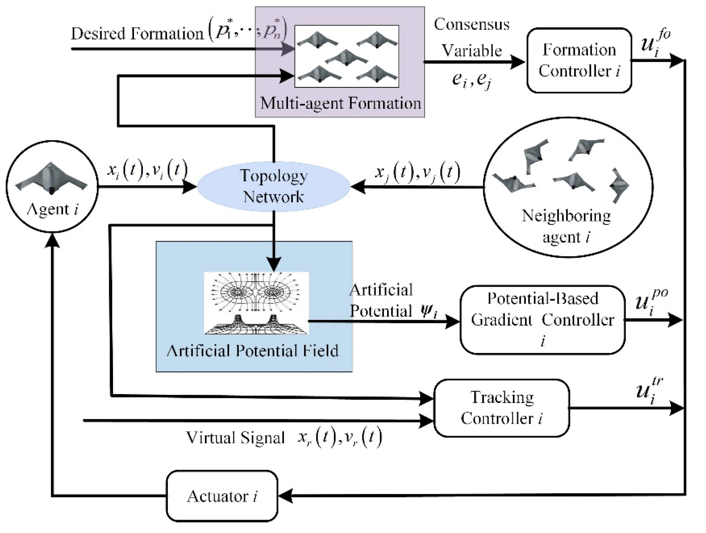
3.1. Controller Design

In this subsection, the distributed formation tracking controller designed for multi-agent systems is composed of three components: a potential-based gradient term, a formation term, and a navigation term that tracks the trajectory signal. Among them, the potential-based gradient term is the negative gradient of the collective potential function, which can ensure collision avoidance and connectivity maintenance between multiple agents. The schematic diagram formation tracking control protocol is shown in Figure 3.

The distributed control protocol of agent i is designed in the same way as the control input form in [23]:

$$u_i=u_i^{po}+u_i^{fo}+u_i^{tr}$$

(10)

where $u_i^{po}$, $u_i^{fo}$, and $u_i^{tr}$ represent potential-based gradient control inputs, formation control inputs, and navigation control inputs, respectively.

Remark 5.

In the distributed control protocol (10), the $u_i^{po}$ is used to avoid collisions between agents and maintain network connectivity; the formation control term $u_i^{fo}$ is used to realize the predetermined pattern of the agents; and $u_i^{tr}$ is used to control the multi-agent to track the time-varying trajectory. The detailed design procedure for the three control items is as follows:

3.1.1. Potential-Based Gradient Term

Each agent must avoid colliding with others during the movement, and one of the key tools for resolving this problem is the artificial potential field (APF). It is used by more local and foreign researchers due to its ability to manage collision issues in real time with less tunable parameters.

There are attractive and repulsive potential fields around each agent. As shown in Figure 4a, when two agents i and j are close to the edge of the collision avoidance radius r_out of each other, the potential field of agent j does not affect agent i, that is, f_rep = 0 (f_rep is the repulsive force). They continue to move and enter the collision avoidance area of each other. Agent i triggers the repulsion potential field of agent j and is repelled by agent j, i.e., f_rep ≠ 0. Furthermore, agent j is repulsed by agent i. In Figure 4b, d_ij = 2r_in represents the collision between agent i and agent j. At the same time, the corresponding repulsive force f_rep = ∞. Therefore, the scope of work of the repulsive potential field is (2r_in, r_in + r_out), which can also be considered as a collision buffer.

In real problems, the network topology is generally time-varying and disconnected. Agent j, for instance, is inside the radius R of agent i at time t (t ≥ t₀). It is possible for it to be outside of the communication radius R of agent i at time t + 1 because of the movement of agent j, resulting in a time-varying neighbor set for agent i. As a result, connectivity maintenance is one of the primary challenges for formation control.

One can also constrain the agent which is within the neighborhood of agent i to the radius R by constructing an attractive potential field. Agent i (see Figure 4) will be attracted by the force generated by the attractive potential field of agent j if agent j is about to pass beyond the radius R of agent i, i.e., d_ij ≥ R. The area of action of the attractive potential field is (r_in + r_out, R).

Based on earlier collision avoidance and connection maintenance analysis, agents i and j repel each other when d_ij < r_in + r_out, and attract each other when d_ij > r_in + r_out. As a result, r_in + r_out is the global minimum of the potential field.

Definition 1.

To be defined as a differentiable collective potential function of κ, it must meet the two conditions mentioned below: 1) As κ = 2r_in, the function tends to infinity and decreases strictly monotonically as (2r_in, r_in + r_out); and 2) it is increases on (r_in + r_out, R), and terminates at R.

According to Definition 1, the action function is

$$\varphi \left(\kappa \right)=\left\{\begin{array}{ll}-\frac{k\left(\kappa -\left(r_{in}+r_{out}\right)\right)\left(\kappa -R\right)}{\left(\kappa -2r_{in}\right)}, & \kappa \in \left(2r_{in},R\right]\\ 0,& \kappa \in \left(R,+\infty \right)\end{array}\right.$$

(11)

where k is a positive coefficient. The collective potential function between agent i and agent j is defined as:

$${\psi }_{ij}\left(\kappa \right)={\displaystyle {\int }_{r_{in}+r_{out}}^{\kappa }\varphi \left(s\right)}ds$$

(12)

The potential energy of the whole multi-agent system can be induced from (12) in the form:

$$E_p=\frac{1}{2}{\displaystyle \sum _{i=1}^n{\displaystyle \sum _{j\in N_i}{a}_{ij}{\psi }_{ij}\left(d_{ij}\right)}}$$

(13)

The negative gradient direction of the collective potential function is defined as the potential force. Under the effect of the neighbor set, the potential-based control input of the agent i can be derived by using (8), (11), and (12):

$$u_i^{po}=-{\displaystyle \sum _{j\in N_i}{a}_{ij}{\nabla }_{x_i}{\psi }_{ij}\left(d_{ij}\right)}$$

(14)

where ∇_xiψ_ij(d_ij) indicates the gradient of ψ_ij(d_ij) along x_i.

3.1.2. Formation Term

In the global coordinate framework, the formation of multi-agents is defined as $p^{*}=\left[{\left(p_1^{*}\right)}^{\mathrm{T}},\cdots ,{\left(p_n^{*}\right)}^{\mathrm{T}}\right]\in {\left({ℝ}^m\right)}^n$, and the distance of any two adjacent agents is given by a (a > 0). We can determine the coordinate representations of other agents in the global coordinate system from any coordinate position $p_1^{*}$ of agent 1 based on the given desired formation shape and the minimal distance a. For example, consider an equilateral triangular formation of six agents in a planer:

In Figure 5, supposing that the position of agent 1 is (x, y), the formation coordinate is

$$p^{*}=\left[{\left(x,y\right)}^{\mathrm{T}},{\left(x+a,y\right)}^{\mathrm{T}},{\left(x+2a,y\right)}^{\mathrm{T}},{\left(x+a/2,y+\left(\sqrt{3}a\right)/2\right)}^{\mathrm{T}},\right.{\left.{\left(x+3a/2,y+\left(\sqrt{3}a\right)/2\right)}^{\mathrm{T}},{\left(x+a,y+\sqrt{3}a\right)}^{\mathrm{T}}\right]}^{\mathrm{T}}$$

Remark 6.

It is noteworthy that the task of agent 1 here differs from that of the virtual leader in [23], which not only leads to the formation but also navigates other agents. In this paper, agent 1 is merely employed as the basis of the formation structure, and we place more emphasis on the relativity of multi-agent position.

Remark 7.

In APF analysis, r_in + r_out is the global minimum point in agent potential field. Agent i is either repelled or attracted when d_ij < R and d_ij ≠ r_in + r_out, so it is a stable point in the potential field at r_in + r_out. As a result, the distance between neighboring agents in the formation must be adjusted to r_in + r_out.

The following is the constraint for formation control:

$$r_{in}+r_{out}=a$$

(15)

Once the formation pattern is achieved and maintained, then there is

$$\begin{array}{l}{v}_i=v_j\\ x_i-p_i^{*}=x_j-p_j^{*} i,j\in \upsilon \end{array}$$

(16)

Set $e_i{ = x}_i{ - p}_i^{*}$ as the formation consensus variable. Therefore, we take the difference of consensus variables and velocity as feedback inputs, and we have

$$u_i^{fo}=-{\displaystyle \sum _{j\in N_i}{k}_1{a}_{ij}\left(e_i-e_j\right)}-{\displaystyle \sum _{j\in N_i}{k}_2{a}_{ij}\left(v_i-v_j\right)}$$

(17)

where (v_i − v_j) is the velocity consensus term between the agent i and its neighbors, k₁ = 1/m and k₂ = 1 s/m.

Remark 8.

Note that the k₁ and k₂ on the right in (17) are to align the units of the relative displacement variable and the relative velocity variable. The two terms on the right of (17) are distinct and can’t be directly added together, according to the principle of mathematics. However, their consistency is what we are primarily interested in this paper. As a result, we ignore them in later processing.

3.1.3. Navigation Term

According to the virtual leader dynamics in (2) and the leader control input in [28], the navigation item control input of agent i is

$$u_i^{tr}=-\left(e_i-x_r\right)-\left(v_i-v_r\right)+f_r$$

(18)

Remark 9.

In this paper, we assume that all agents have knowledge of the virtual leader. However, generally speaking, each agent does not know the state variables of the virtual leader during the formation process. For example, when multiple UAVs form an encirclement monitoring situation for the target to improve the cooperative efficiency, the leader is considered a non-cooperative target, and its control input and state are usually unknown to all followers. Therefore, it is necessary to design an observer for each agent to estimate the state of the leader. It is a pity that we didn’t do this, and it will be the main focus of the next work.

3.2. Stability Analysis

Theorem 1.

Consider a system of n mobile agents, each of which is modeled by (1) and is steered by the control protocol (10). If the initial energy E(t₀) of the system is finite (i.e., E(t₀) = c, c > 0 is a constant), then

1 

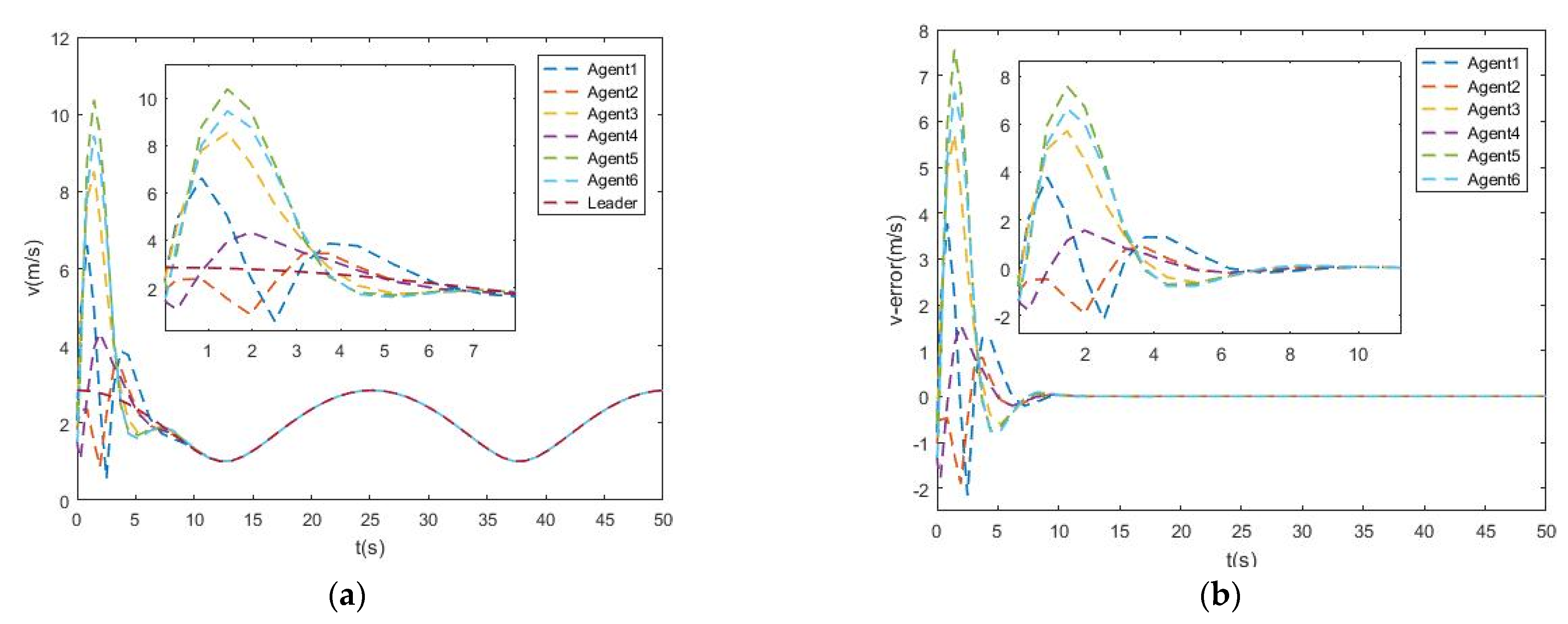
All of the velocities of agents asymptotically approach the velocity of the virtual leader, i.e.,$v_1=v_2=\cdots =v_n=v_r$

2 

The multi-agent system eventually approaches a positional structure$x^{*}$, which is the global minimum of the artificial potentials energy E_p(x), i.e.,$E_p\left(x^{*}\right)=\underset{x}{\min }\left\{E_p\left(x\right),\forall t\ge t_0\right\}$

3 

There are no collisions between any two mobile agents: d_ij > 2r_in ∀t ≥ t₀, for i, j ∈ υ, i ≠ j.

Proof of Theorem 1. Part 1

: define the energy function:

$$E=\frac{1}{2}{\displaystyle \sum _{i=1}^n\left[{\left(v_i-v_r\right)}^{\mathrm{T}}\left(v_i-v_r\right)+{\displaystyle \sum _{j\in N_i}{a}_{ij}{\psi }_{ij}\left(d_{ij}\right)}\right.}\left.+{\left(e_i-x_r\right)}^{\mathrm{T}}\left(e_i-x_r\right)+\frac{1}{2}{\displaystyle \sum _{j\in N_i}{a}_{ij}{\left(e_i-e_j\right)}^{\mathrm{T}}\left(e_i-e_j\right)}\right]$$

(19)

Let

$$\left\{\begin{array}{l}{\tilde{x}}_i=e_i-x_r\\ {\tilde{v}}_i=v_i-v_r\\ {\tilde{x}}_{ij}={\tilde{x}}_i-{\tilde{x}}_j.\end{array}\right.$$

(20)

Take (21) into (10) and (20), and then the control protocol of agent i and the energy function of the system are adjusted into

$$u_i=-{\displaystyle \sum _{j\in N_i}{a}_{ij}{\nabla }_{{\tilde{x}}_i}{\psi }_{ij}\left(‖{\tilde{x}}_{ij}+p_{ij}^{*}‖\right)}-{\displaystyle \sum _{j\in N_i}{a}_{ij}\left({\tilde{x}}_i-{\tilde{x}}_j\right)}-{\displaystyle \sum _{j\in N_i}{a}_{ij}\left({\tilde{v}}_i-{\tilde{v}}_j\right)}-{\tilde{v}}_i-{\tilde{x}}_i+f_r$$

(21)

$$E=\frac{1}{2}{\displaystyle \sum _{i=1}^n\left[{\tilde{v}}_i^{\mathrm{T}}{\tilde{v}}_i+{\displaystyle \sum _{j\in N_i}{a}_{ij}\psi \left(‖{\tilde{x}}_{ij}+p_{ij}^{*}‖\right)}\right.}\left.+{\tilde{x}}_i^{\mathrm{T}}{\tilde{x}}_i+\frac{1}{2}{\displaystyle \sum _{j\in N_i}{a}_{ij}{\left({\tilde{x}}_i-{\tilde{x}}_j\right)}^{\mathrm{T}}\left({\tilde{x}}_i-{\tilde{x}}_j\right)}\right]$$

(22)

where $d_{ij}=\Vert {\tilde{x}}_{ij}+p_{ij}^{*}\Vert$ and $e_i{-e}_j={\tilde{x}}_i-{\tilde{x}}_j$. The time derivative of Equation (23) is

$$\begin{array}{cc}\hfill \dot{E}& =\frac{1}{2}{\displaystyle \sum _{i=1}^n\left[2{\tilde{v}}_i^{\text{T}}{\dot{\tilde{v}}}_i+2{\tilde{v}}_i^{\text{T}}{\displaystyle \sum _{j\in N_i}{a}_{ij}{\nabla }_{{\tilde{x}}_i}{\psi }_{ij}\left(‖{\tilde{x}}_{ij}+p_{ij}^{*}‖\right)}\right.}\left.+2{\tilde{v}}_i^{\text{T}}{\tilde{x}}_i+{\displaystyle \sum _{j\in N_i}{a}_{ij}{\left({\tilde{v}}_i-{\tilde{v}}_j\right)}^{\text{T}}\left({\tilde{x}}_i-{\tilde{x}}_j\right)}\right]\hfill \\ \hfill & \text{=}{\displaystyle \sum _{i=1}^n\left[{\tilde{v}}_i^{\text{T}}\left(u_i-f_r\right)+{\tilde{v}}_i^{\text{T}}{\displaystyle \sum _{j\in N_i}{a}_{ij}{\nabla }_{{\tilde{x}}_i}{\psi }_{ij}\left(‖{\tilde{x}}_{ij}+p_{ij}^{*}‖\right)}\right.}\left.+{\tilde{v}}_i^{\text{T}}{\tilde{x}}_i+\frac{1}{2}{\displaystyle \sum _{j\in N_i}{a}_{ij}{\left({\tilde{v}}_i-{\tilde{v}}_j\right)}^{\text{T}}\left({\tilde{x}}_i-{\tilde{x}}_j\right)}\right]\hfill \end{array}$$

(23)

where ${\nabla }_{{\tilde{x}}_i}{\mathsf{\psi }}_{ij}=\partial {\mathsf{\psi }}_{ij}/\partial {\tilde{x}}_i$. Substituting u_i from (22) into (24), one obtains

$$\begin{array}{cc}\hfill \dot{E}& ={\displaystyle \sum _{i=1}^n\left[{\tilde{v}}_i^{\text{T}}\left\{-{\displaystyle \sum _{j\in N_i}{a}_{ij}{\nabla }_{{\tilde{x}}_i}{\psi }_{ij}\left(‖{\tilde{x}}_{ij}+p_{ij}^{*}‖\right)-{\displaystyle \sum _{j\in N_i}{a}_{ij}\left({\tilde{x}}_i-{\tilde{x}}_j\right)}}\right.\right.}\left.-{\displaystyle \sum _{j\in N_i}{a}_{ij}\left({\tilde{v}}_i-{\tilde{v}}_j\right)}-{\tilde{v}}_i-{\tilde{x}}_i\right\}\hfill \\ \hfill & +{\tilde{v}}_i^{\text{T}}{\displaystyle \sum _{j\in N_i}{a}_{ij}{\nabla }_{{\tilde{x}}_i}{\psi }_{ij}\left(‖{\tilde{x}}_{ij}+p_{ij}^{*}‖\right)}\left.+{\tilde{v}}_i^{\text{T}}{\tilde{x}}_i+\frac{1}{2}{\displaystyle \sum _{j\in N_i}{a}_{ij}{\left({\tilde{v}}_i-{\tilde{v}}_j\right)}^{\text{T}}\left({\tilde{x}}_i-{\tilde{x}}_j\right)}\right]\hfill \\ \hfill & \text{=}{\displaystyle \sum _{i=1}^n\left[-{\tilde{v}}_i^{\text{T}}{\displaystyle \sum _{j\in N_i}{a}_{ij}\left({\tilde{x}}_i-{\tilde{x}}_j\right)}-{\tilde{v}}_i^{\text{T}}{\displaystyle \sum _{j\in N_i}{a}_{ij}\left({\tilde{v}}_i-{\tilde{v}}_j\right)-{\tilde{v}}_i^{\text{T}}{\tilde{v}}_i}\right.}\left.+\frac{1}{2}{\tilde{v}}_i^{\text{T}}{\displaystyle \sum _{j\in N_i}{a}_{ij}\left({\tilde{x}}_i-{\tilde{x}}_j\right)-\frac{1}{2}{\displaystyle \sum _{j\in N_i}{a}_{ij}{\tilde{v}}_j^{\text{T}}\left({\tilde{x}}_i-{\tilde{x}}_j\right)}}\right]\hfill \\ \hfill & \text{=}{\displaystyle \sum _{i=1}^n\left[-{\tilde{v}}_i^{\text{T}}{\displaystyle \sum _{j\in N_i}{a}_{ij}\left({\tilde{v}}_i-{\tilde{v}}_j\right)}-{\tilde{v}}_i^{\text{T}}{\tilde{v}}_i\right.}\left.-\frac{1}{2}{\tilde{v}}_i^{\text{T}}{\displaystyle \sum _{j\in N_i}{a}_{ij}\left({\tilde{x}}_i-{\tilde{x}}_j\right)}-\frac{1}{2}{\displaystyle \sum _{j\in N_i}{a}_{ij}{\tilde{v}}_j^{\text{T}}\left({\tilde{x}}_i-{\tilde{x}}_j\right)}\right]\hfill \end{array}$$

(24)

Since the topology between multi-agents in this paper is undirected, the adjacency matrix A and the Laplace matrix L are symmetric. One can obtain

$$-{\displaystyle \sum _{i=1}^n{\tilde{v}}_i^{\mathrm{T}}}{\displaystyle \sum _{j\in N_i}{a}_{ij}\left({\tilde{v}}_i-{\tilde{v}}_j\right)}=-{\tilde{v}}^{\mathrm{T}}\left(L\otimes I_m\right)\tilde{v}$$

(25)

$$-{\displaystyle \sum _{i=1}^n{\tilde{v}}_i^{\mathrm{T}}{\tilde{v}}_i}=-{\tilde{v}}^{\mathrm{T}}\left(I_n\otimes I_m\right)\tilde{v}$$

(26)

$$-{\displaystyle \sum _{i=1}^n{\tilde{v}}_i^{\mathrm{T}}}{\displaystyle \sum _{j\in N_i}{a}_{ij}\left({\tilde{x}}_i-{\tilde{x}}_j\right)=-{\tilde{v}}^{\mathrm{T}}}\left(L\otimes I_m\right)\tilde{x}$$

(27)

$$-{\displaystyle \sum _{i=1}^n{\displaystyle \sum _{j\in N_i}{a}_{ij}{\tilde{v}}_j^{\mathrm{T}}\left({\tilde{x}}_i-{\tilde{x}}_j\right)}}={\tilde{v}}^{\mathrm{T}}\left(L\otimes I_m\right)\tilde{x}$$

(28)

where $\tilde{v} ={\left[{\tilde{v}}_1^{\mathrm{T}}, \cdots {, \tilde{v}}_n^{\mathrm{T}}\right]}^{\mathrm{T}}\in {ℝ}^{mn}$, $\tilde{x} ={\left[{\tilde{x}}_1^{\mathrm{T}}, \cdots {, \tilde{x}}_n^{\mathrm{T}}\right]}^{\mathrm{T}}\in {ℝ}^{mn}$. I_n ∈ ℝ^n×n and I_m ∈ ℝ^m×m are the identity matrix. L⊗I_m denotes Kronecker product of L and I_m. Thus, (25) can be written as

$$\dot{E}=-{\tilde{v}}^{\mathrm{T}}\left[\left(L+I_n\right)\otimes I_m\right]\tilde{v}\le 0$$

(29)

Considering L is a positive semi-definite matrix and I_n is a positive definite matrix, (L + I_n) is a positive definite matrix in (30). Therefore, the fact $\dot{E} \le 0$ reveals that the energy E(t) of the multi-agent system is a non-increasing function of time t (E(t) ≤ E(t₀) = c, ∀t ≥ t₀). Take into account the collective relative dynamics of multi-agents using (1) and (21).

$$\left\{\begin{array}{l}\dot{\tilde{x}}=\tilde{v}\\ \dot{\tilde{v}}=-{\nabla }_x{E}_p-\left[\left(L+I_n\right)\otimes I_m\right]e-\left[\left(L+I_n\right)\otimes I_m\right]v\\ +\left(1\otimes I_m\right)v_r+\left(1\otimes I_m\right)x_r\end{array}\right.$$

(30)

where ∇_xE_p represents the gradient of (13) with respect to x. ${e=[e}_1^{\mathrm{T}},\cdots {,e}_n^{\mathrm{T}}]$ and 1 is the n-vector of ones.

Set ${\mathsf{\Omega }}_{\mathrm{c}}=\left\{\left(\tilde{x},\tilde{v}\right): E\left(\tilde{x},\tilde{v}\right)\le c\right\}$ be a set of (23) of (31) such that, for any solution starting in Ω_c, the agents form a shape of regular formation. Since $\dot{E}\le 0$, the set Ω_c is an invariant set. From Lemma 2, all the solutions of (31) starting from Ω_c will converge to the largest invariant set $\overline{\Omega }=\left\{\left(\tilde{x},\tilde{v}\right){\Omega }_c\text{:} \dot{E} =0\right\}$. Based on (30), one can obtain

$$\dot{E}=-{\tilde{v}}^{\mathrm{T}}\left[\left(L+I_n\right)\otimes I_m\right]\tilde{v}=0$$

(31)

Hence, $\tilde{v} = 0$ is equivalent to $v_1{=v}_2=\cdots {=v}_n{=v}_r$, which shows the velocities of all agents ultimately converge on the velocity of the virtual leader. This completes the proof of component (1).

Part 2: Let

$$U_i\left(x_i\right)={\displaystyle \sum _{j\in N_i}{a}_{ij}{\psi }_{ij}\left(d_{ij}\right)}+{\left(e_i-x_r\right)}^{\mathrm{T}}\left(e_i-x_r\right)+\frac{1}{2}{\displaystyle \sum _{j\in N_i}{a}_{ij}}{\left(e_i-e_j\right)}^{\mathrm{T}}\left(e_i-e_j\right)$$

(32)

According to (20) one has

$$E=\frac{1}{2}{\displaystyle \sum _{i=1}^n\left[{\left(v_i-v_r\right)}^{\mathrm{T}}\left(v_i-v_r\right)+U_i\left(x_i\right)\right]}$$

(33)

Part (1) shows that, while the system is in a steady state, ${\dot{x}}_1{=\dot{x}}_2=\cdots {=\dot{x}}_n{=\dot{x}}_r$ and E is a constant. Therefore, differentiating (34) with respect to t, one obtains

$$\begin{array}{cc}\hfill \frac{1}{2}{\displaystyle \sum _{i=1}^n{\dot{U}}_i\left(x_i\right)}& =\frac{1}{2}{\displaystyle \sum _{i=1}^n\left[v_i^{\mathrm{T}}{\displaystyle \sum _{j\in N_i}{a}_{ij}{\nabla }_{x_i}{\psi }_{ij}+2{\left(v_i-v_r\right)}^{\mathrm{T}}\left(e_i-x_r\right)}\right.}\left.+{\displaystyle \sum _{j\in N_i}{a}_{ij}{\left(v_i-v_r\right)}^{\mathrm{T}}\left(e_i-e_j\right)}\right]\hfill \\ \hfill & =\frac{1}{2}{\displaystyle \sum _{i=1}^n\left[v_i^{\mathrm{T}}{\displaystyle \sum _{j\in N_i}{a}_{ij}{\nabla }_{x_i}{\psi }_{ij}}\right]}=0\hfill \end{array}$$

(34)

where $v_i\ne 0$, so ${\displaystyle \sum }_{{j\in }_{Ni}}{a}_{ij}{\nabla }_{{\tilde{x}}_i}{\psi }_{ij}=0$, which shows that the formation asymptotically converges to a stable configuration that is an extreme minimum of the total artificial potential energy. This completes the proof of component (2).

Part 3:

Assume, using the contradicting strategy, that any two agents, k and l (k,l∈υ,k≠l) collide at time t(t > t₀), i.e., $\Vert x_k\left(t\right){-x}_l\left(t\right)\Vert \le {2r}_{in}$. Then

$$E_p=\frac{1}{2}{\displaystyle \sum _{i=1}^n{\displaystyle \sum _{j\in N_i}{a}_{ij}\psi \left(d_{ij}\right)}} =a_{kl}\psi \left(d_{kl}\right)+\frac{1}{2}{\displaystyle \sum _{i\in \nu \backslash \left\{k,l\right\}}^n{\displaystyle \sum _{j\in N_i\backslash \left\{k,l\right\}}{a}_{ij}}}\psi \left(d_{ij}\right)\ge a_{kl}\psi \left(d_{kl}\right)$$

(35)

It is known from the proof in Part (1) that

$$a_{kl}\psi \left(d_{kl}\right)<E_p<E\le c$$

(36)

However, ${\psi }_{ij}{(d}_{\mathit{kl}})\to \infty$ as $\Vert { x}_k\left(t\right){-x}_l\left(t\right)\Vert \to {2r}_{in}$. (37) contradicts $\Vert x_k\left(t\right){-x}_l\left(t\right)\Vert \le {2r}_{in}$, and the assumption is invalid. As a consequence, no collision occurs throughout the multi-agent formation process. This completes the proof of component (3). □

4. Numerical Simulation

In this section, six agents achieve an equilateral triangle formation and a hexagon formation by utilizing the proposed control algorithm (10) in the simulation environment of 2016 Matlab/Simulink¹. We consider the gradient term based on the potential in the equilateral triangle formation, but not in the hexagon formation. By comparison, we can know whether or not multiple rigid agents collide. The Laplacian matrix rank is used to quantify the connectivity between multiple agents.

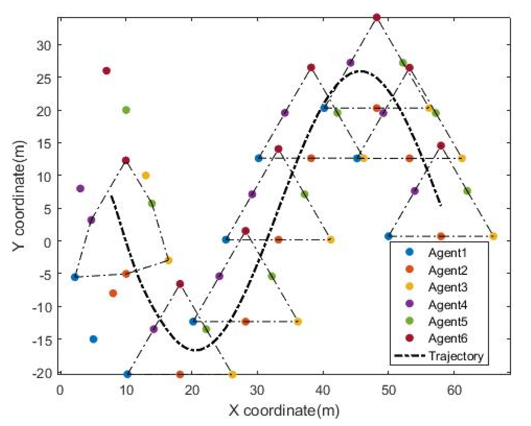
4.1. An Equilateral Triangle Formation

The start position vectors of six agents are specified as x₁(t₀) = [5, −15]^T, x₂(t₀) = [8, −8]^T, x₃(t₀) = [13, 10]^T, x₄(t₀) = [3, 8]^T, x₅(t₀) = [10, 20]^T, x₆(t₀) = [7, 26]^T, and the initial velocity are chosen at random from box [−2, 2]² m/s. The virtual leader trajectory is x_r = [t, −64sin(t/8)/3]^T, with x_r(t₀) = [0, 0]^T and v_r(t₀) = [1, −8/3]^T being the original position and velocity vectors, respectively.

Moreover, the body radius of each agent is r_in = 3 m, anti-collision radius r_out = 5 m, and sensing radius R = 10 m. The action function coefficient, k = 0.02. The next is the diagram equilateral triangle formation of the six agents.

The formation process of six agents is displayed in Figure 6, with the solid dots representing the agents and the black dotted line illustrating the motion trajectory. It can be seen that, in the initial state, all agents are driven by the control algorithm to gather. They finally form a stable equilateral triangle formation and move along a sinusoidal trajectory after that.

Figure 7 shows the internal distances between any two agents, and (d_ij)_min > 2r_in = 6 m implies that they did not collide during the movement because of the artificial potential field. The internal distances between the agents converge to three values, 8 m, 13.68 m, and 16 m, when the multi-agent formation is maintained. The predefined equilateral triangle configuration can also be used to verify it.

Figure 8a indicates the velocity of the multi-agent and virtual leader fluctuations, and the velocity of all agents matches the virtual curve of the leader at system stability. It is further confirmed by Figure 8b, which demonstrates that the agent can track the velocity of the virtual leader successfully during connectivity maintenance and collision avoidance.

Figure 9 clearly shows the control input in x- and y-directions for each agent. The movement of the agent is a sinusoidal trajectory, which can be decomposed into a constant speed motion on the x-axis and a regular fluctuation on the y-axis. Therefore, the corresponding control inputs are 0 and slightly sinusoidal, respectively.

It can be seen from Lemma 1 that, when the rank of the Laplacian matrix corresponding to n agents is n-1, the graph is connected. In Figure 10, the rank of the Laplacian matrix is 5 after the formation is stable, which indicates that the topological network is connected, and the purpose of maintaining connectivity is achieved.

4.2. A Hexagon Formation

In this example, a hexagonal formation, which is also composed of six agents, was used to verify the control scheme that is missing a potential-based term in (10) and in the case of the potential function of [28]. The initial position vector, velocity vector, and all parameters are the same as in the above example. The simulation results are as follows:

As seen in Figure 11, six agents completed the hexagonal formation task. However, in Figure 12, (d_ij)_min < 2r_in = 6 m, suggesting that, in the two scenarios mentioned above, multiple agents collided. This demonstrates the effectiveness of algorithm (10) proposed in this study. In addition, the velocity of the multi-agent also tracks the velocity of the virtual leader in Figure 13a,b.

5. Conclusions

In this paper, a displacement-based formation control problem was considered for the multi-agent system. Since the distance between multi-agents is either close or remote during movement, they will unavoidably collide or lose contact, which motivates the research of collision avoidance and connectivity maintenance. In [28], the author separately addressed these problems by establishing two respective potential functions, both of which included sophisticated design variables. Instead, we only employed one potential function with one coefficient. The two simulation results demonstrated that the distributed controller with provable stability can guarantee collision avoidance and connectivity maintenance between multi-agents while achieving formation.

In the future, this paper is to extend the control protocol to the following situations: considering uncertainties or disturbances in agent dynamics; designing an observer for the virtual leader; and obstacle avoidance.

The simulation figures receive legal protection from the department.

References

- Reynolds, C.W. Flocks, herds and schools: A distributed behavioral model. In Proceedings of the 14th Annual Conference on Computer Graphics and Interactive Techniques, Anaheim, CA, USA, 1 August 1987; pp. 25–34. [Google Scholar]
- Dorri, A.; Kanhere, S.S.; Jurdak, R. Multi-Agent Systems: A Survey. IEEE Access 2018, 6, 28573–28593. [Google Scholar] [CrossRef]
- Litimein, H.; Huang, Z.-Y.; Hamza, A. A Survey on Techniques in the Circular Formation of Multi-Agent Systems. Electronics 2021, 10, 2959. [Google Scholar] [CrossRef]
- Wang, C.; Tnunay, H.; Zuo, Z.; Lennox, B.; Ding, Z. Fixed-time formation control of multirobot systems: Design and experiments. IEEE Trans. Ind. Electron. 2018, 66, 6292–6301. [Google Scholar] [CrossRef]
- Cheng, W.; Zhang, K.; Jiang, B.; Ding, S.X. Fixed-Time Formation Tracking for Heterogeneous Multi-Agent Systems under Actuator Faults and Directed Topologies. IEEE Trans. Aerosp. Electron. Syst. 2022, 58, 3063–3077. [Google Scholar] [CrossRef]
- Yan, D.; Zhang, W.; Chen, H. Design of a Multi-Constraint Formation Controller Based on Improved MPC and Consensus for Quadrotors. Aerospace 2022, 9, 94. [Google Scholar] [CrossRef]
- Saif, A.W.; Alabsari, N.; Ferik, S.E.; Elshafei, M. Formation control of quadrotors via potential field and geometric techniques. Int. J. Adv. Appl. Sci. 2020, 7, 82–96. [Google Scholar] [CrossRef]
- Yuan, C.; Licht, S.; He, H. Formation learning control of multiple autonomous underwater vehicles with heterogeneous non-linear uncertain dynamics. IEEE Trans. Cybern. 2018, 48, 2920–2934. [Google Scholar] [CrossRef]
- Ren, W.; Atkins, E. Distributed multi-vehicle coordinated control via local information exchange. Int. J. Robust Nonlinear Control IFAC Affiliated J. 2007, 17, 1002–1033. [Google Scholar] [CrossRef]
- Oh, K.-K.; Ahn, H.-S. Formation Control and Network Localization via Orientation Alignment. IEEE Trans. Autom. Control 2013, 59, 540–545. [Google Scholar] [CrossRef]
- Babazadeh, R.; Selmic, R. Distance-Based Multiagent Formation Control with Energy Constraints Using SDRE. IEEE Trans. Aerosp. Electron. Syst. 2019, 56, 41–56. [Google Scholar] [CrossRef]
- Aryankia, K.; Selmic, R.R. Neural Network-Based Formation Control with Target Tracking for Second-Order Nonlinear MultiAgent Systems. IEEE Trans. Aerosp. Electron. Syst. 2022, 58, 328–341. [Google Scholar] [CrossRef]
- Trinh, M.H.; Zhao, S.; Sun, Z.; Zelazo, D.; Anderson, B.D.; Ahn, H.-S. Bearing-Based Formation Control of A Group of Agents with Leader-First Follower Structure. IEEE Trans. Autom. Control 2018, 64, 598–613. [Google Scholar] [CrossRef]
- Luo, X.; Li, X.; Guan, X. Bearing-only formation control of multi-agent systems in local reference frames. Int. J. Control 2021, 94, 1261–1272. [Google Scholar] [CrossRef]
- Li, X.; Wen, C.; Chen, C. Adaptive Formation Control of Networked Robotic Systems with Bearing-Only Measurements. IEEE Trans. Cybern. 2020, 51, 199–209. [Google Scholar] [CrossRef]
- Ge, X.; Han, Q.L. Distributed formation control of networked multi-agent systems using a dynamic event-triggered commu-nication mechanism. IEEE Trans. Ind. Electro. 2017, 64, 8118–8127. [Google Scholar] [CrossRef]
- Yu, H.; Shi, P.; Lim, C.-C.; Wang, D. Formation control for multi-robot systems with collision avoidance. Int. J. Control 2019, 92, 2223–2234. [Google Scholar] [CrossRef]
- Wang, J.; Han, L.; Dong, X.; Li, Q.; Ren, Z. Distributed sliding mode control for time-varying formation tracking of multi-UAV system with a dynamic leader. Aerosp. Sci. Technol. 2021, 111, 106549. [Google Scholar] [CrossRef]
- Oh, K.-K.; Park, M.-C.; Ahn, H.-S. A survey of multi-agent formation control. Automatica 2015, 53, 424–440. [Google Scholar] [CrossRef]
- Khatib, O. Real-time obstacle avoidance for manipulators and mobile robots. In Autonomous Robot Vehicles; Cox, I.J., Wilfong, G.T., Eds.; Springer: New York, NY, USA, 1986; Volume 5, pp. 396–404. [Google Scholar] [CrossRef]
- Olfati-Saber, R. Flocking for Multi-Agent Dynamic Systems: Algorithms and Theory. IEEE Trans. Autom. Control 2006, 51, 401–420. [Google Scholar] [CrossRef]
- Do, K.D. Formation Tracking Control of Unicycle-Type Mobile Robots with Limited Sensing Ranges. IEEE Trans. Control Syst. Technol. 2008, 16, 527–538. [Google Scholar] [CrossRef]
- Shi, Q.; Li, T.; Li, J.; Chen, C.P.; Xiao, Y.; Shan, Q. Adaptive leader-following formation control with collision avoidance for a class of second-order nonlinear multi-agent systems. Neurocomputing 2019, 350, 282–290. [Google Scholar] [CrossRef]
- Liu, Y.; Huang, P.; Zhang, F.; Zhao, Y. Distributed formation control using artificial potentials and neural network for constrained multiagent systems. IEEE Trans. Control Syst. Technol. 2018, 28, 697–704. [Google Scholar] [CrossRef]
- Yan, T.; Xu, X.; Li, Z.; Li, E. Flocking of multi-agent system with dynamic topology by pinning control. IET Control Theory Appl. 2020, 14, 3374–3381. [Google Scholar] [CrossRef]
- Tanner, H.G.; Jadbabaie, A.; Pappas, G.J. Flocking in Fixed and Switching Networks. IEEE Trans. Autom. Control 2007, 52, 863–868. [Google Scholar] [CrossRef]
- Mondal, A.; Behera, L.; Sahoo, S.R.; Shukla, A. A novel multi-agent formation control law with collision avoidance. IEEE/CAA J. Autom. Sin. 2017, 4, 558–568. [Google Scholar] [CrossRef]
- Mondal, A.; Bhowmick, C.; Behera, L.; Jamshidi, M. Trajectory tracking by multiple agents in formation with collision avoidance and connectivity assurance. IEEE Syst. J. 2017, 12, 2449–2460. [Google Scholar] [CrossRef]
- Pan, Z.; Zhang, C.; Xia, Y.; Xiong, H.; Shao, X. An Improved Artificial Potential Field Method for Path Planning and Formation Control of the Multi-UAV Systems. IEEE Trans. Circuits Syst. II Express Briefs 2021, 69, 1129–1133. [Google Scholar] [CrossRef]
- Shou, Y.; Xu, B.; Lu, H.; Zhang, A.; Mei, T. Finite-time formation control and obstacle avoidance of multi-agent system with application. Int. J. Robust Nonlinear Control 2022, 32, 2883–2901. [Google Scholar] [CrossRef]
- González-Sierra, J.; Dzul, A.; Ríos, H. Robust sliding-mode formation control and collision avoidance via repulsive vector fields for a group of Quad-Rotors. Int. J. Syst. Sci. 2019, 50, 1483–1500. [Google Scholar] [CrossRef]
- Liu, Y.; Passino, K.; Polycarpou, M. Stability analysis of M-dimensional asynchronous swarms with a fixed communication topology. IEEE Trans. Autom. Control 2003, 48, 76–95. [Google Scholar] [CrossRef]
- Li, D.; Zhang, W.; He, W.; Li, C.; Ge, S.S. Two-Layer Distributed Formation-Containment Control of Multiple Euler–Lagrange Systems by Output Feedback. IEEE Trans. Cybern. 2018, 49, 675–687. [Google Scholar] [CrossRef] [PubMed]
- Trejo, J.A.V.; Rotondo, D.; Theilliol, D.; Medina, M.A. Observer-based quadratic boundedness leader-following control for multi-agent systems. Int. J. Control 2022, 1–10. [Google Scholar] [CrossRef]
- Xiong, T.; Gu, Z. Observer-based adaptive fixed-time formation control for multi-agent systems with unknown uncertainties. Neurocomputing 2021, 423, 506–517. [Google Scholar] [CrossRef]
- Zhao, W.; Liu, H.; Valavanis, K.P.; Lewis, F.L. Fault-Tolerant Formation Control for Heterogeneous Vehicles Via Reinforcement Learning. IEEE Trans. Aerosp. Electron. Syst. 2021, 58, 2796–2806. [Google Scholar] [CrossRef]
- Dong, X.; Zhou, Y.; Ren, Z.; Zhong, Y. Time-Varying Formation Tracking for Second-Order Multi-Agent Systems Subjected to Switching Topologies with Application to Quadrotor Formation Flying. IEEE Trans. Ind. Electron. 2016, 64, 5014–5024. [Google Scholar] [CrossRef]
- Han, T.; Lin, Z.; Zheng, R.; Fu, M. A Barycentric Coordinate-Based Approach to Formation Control Under Directed and Switching Sensing Graphs. IEEE Trans. Cybern. 2017, 48, 1202–1215. [Google Scholar] [CrossRef] [PubMed]
- Zavlanos, M.M.; Pappas, G.J. Potential Fields for Maintaining Connectivity of Mobile Networks. IEEE Trans. Robot. 2007, 23, 812–816. [Google Scholar] [CrossRef]
- Li, X.; Sun, D.; Yang, J. A bounded controller for multirobot navigation while maintaining network connectivity in the presence of obstacles. Automatica 2013, 49, 285–292. [Google Scholar] [CrossRef]
- Xu, Y.; Wang, C.; Cai, X.; Li, Y.; Xu, L. Output-feedback formation tracking control of networked nonholonomic multi-robots with connectivity preservation and collision avoidance. Neurocomputing 2020, 414, 267–277. [Google Scholar] [CrossRef]
- Fu, J.; Wen, G.; Yu, X.; Wu, Z.-G. Distributed Formation Navigation of Constrained Second-Order Multiagent Systems With Collision Avoidance and Connectivity Maintenance. IEEE Trans. Cybern. 2020, 52, 2149–2162. [Google Scholar] [CrossRef]
- Dong, Y.; Huang, J. Flocking with connectivity preservation of multiple double integrator systems subject to external disturbances by a distributed control law. Automatica 2015, 55, 197–203. [Google Scholar] [CrossRef]
- Dong, Y.; Su, Y.; Liu, Y.; Xu, S. An internal model approach for multi-agent rendezvous and connectivity preservation with nonlinear dynamics. Automatica 2018, 89, 300–307. [Google Scholar] [CrossRef]
- Peng, Z.; Wang, D.; Li, T.; Han, M. Output-Feedback Cooperative Formation Maneuvering of Autonomous Surface Vehicles with Connectivity Preservation and Collision Avoidance. IEEE Trans. Cybern. 2019, 50, 2527–2535. [Google Scholar] [CrossRef] [PubMed]
- Cong, Y.; Du, H.; Jin, Q.; Zhu, W.; Lin, X. Formation control for multiquadrotor aircraft: Connectivity preserving and collision avoidance. Int. J. Robust Nonlinear Control 2020, 30, 2352–2366. [Google Scholar] [CrossRef]
- Filotheou, A.; Nikou, A.; Dimarogonas, D.V. Robust decentralised navigation of multi-agent systems with collision avoidance and connectivity maintenance using model predictive controllers. Int. J. Control 2020, 93, 1470–1484. [Google Scholar] [CrossRef]
- Dong, X.; Yu, B.; Shi, Z.; Zhong, Y. Time-Varying Formation Control for Unmanned Aerial Vehicles: Theories and Applications. IEEE Trans. Control Syst. Technol. 2014, 23, 340–348. [Google Scholar] [CrossRef]
- Biggs, N.N.; Biggs, L.; Norman, B. Algebraic Graph Theory, 2nd ed.; Cambridge university press: Cambridge, UK, 1993; pp. 7–13. [Google Scholar]
- Caruso, M.J. Applications of magnetic sensors for low cost compass systems. In Proceedings of the IEEE Position Location and Navigation Symposium (Cat. No. 00CH37062), San Diego, CA, USA, 13–16 March 2002; pp. 177–184. [Google Scholar] [CrossRef]
- Khalil, H.K. Lyapunov Stability. In Nonlinear System, 3rd ed.; Prentice Hall: Hoboken, NJ, USA, 2002; Volume 3, pp. 97–154. [Google Scholar]
Publisher’s Note: MDPI stays neutral with regard to jurisdictional claims in published maps and institutional affiliations. |
© 2022 by the authors. Licensee MDPI, Basel, Switzerland. This article is an open access article distributed under the terms and conditions of the Creative Commons Attribution (CC BY) license (https://creativecommons.org/licenses/by/4.0/).
Share and Cite
Qiao, Y.; Huang, X.; Yang, B.; Geng, F.; Wang, B.; Hao, M.; Li, S. Formation Tracking Control for Multi-Agent Systems with Collision Avoidance and Connectivity Maintenance. Drones 2022, 6, 419. https://doi.org/10.3390/drones6120419
Qiao Y, Huang X, Yang B, Geng F, Wang B, Hao M, Li S. Formation Tracking Control for Multi-Agent Systems with Collision Avoidance and Connectivity Maintenance. Drones. 2022; 6(12):419. https://doi.org/10.3390/drones6120419
Chicago/Turabian StyleQiao, Yitao, Xuxing Huang, Bin Yang, Feilong Geng, Bingheng Wang, Mingrui Hao, and Shuang Li. 2022. "Formation Tracking Control for Multi-Agent Systems with Collision Avoidance and Connectivity Maintenance" Drones 6, no. 12: 419. https://doi.org/10.3390/drones6120419
APA StyleQiao, Y., Huang, X., Yang, B., Geng, F., Wang, B., Hao, M., & Li, S. (2022). Formation Tracking Control for Multi-Agent Systems with Collision Avoidance and Connectivity Maintenance. Drones, 6(12), 419. https://doi.org/10.3390/drones6120419