Article

Deep Learning Architecture for UAV Traffic-Density Prediction

by
Abdulrahman Alharbi
*,
Ivan Petrunin
and
Dimitrios Panagiotakopoulos
School of Aerospace, Transport and Manufacturing, Cranfield University, Bedford MK43 0AL, UK
*
Author to whom correspondence should be addressed.
Drones 2023, 7(2), 78; https://doi.org/10.3390/drones7020078
Submission received: 30 November 2022 / Revised: 12 January 2023 / Accepted: 17 January 2023 / Published: 22 January 2023
(This article belongs to the Special Issue AAM Integration: Strategic Insights and Goals)

Abstract

:
The research community has paid great attention to the prediction of air traffic flows. Nonetheless, research examining the prediction of air traffic patterns for unmanned aircraft traffic management (UTM) is relatively sparse at present. Thus, this paper proposes a one-dimensional convolutional neural network and encoder-decoder LSTM framework to integrate air traffic flow prediction with the intrinsic complexity metric. This adapted complexity metric takes into account the important differences between ATM and UTM operations, such as dynamic flow structures and airspace density. Additionally, the proposed methodology has been evaluated and verified in a simulation scenario environment, in which a drone delivery system that is considered essential in the delivery of COVID-19 sample tests, package delivery services from multiple post offices, an inspection of the railway infrastructure and fire-surveillance tasks. Moreover, the prediction model also considers the impacts of other significant factors, including emergency UTM operations, static no-fly zones (NFZs), and variations in weather conditions. The results show that the proposed model achieves the smallest RMSE value in all scenarios compared to other approaches. Specifically, the prediction error of the proposed model is 8.34% lower than the shallow neural network (on average) and 19.87% lower than the regression model on average.

1. Introduction

The low development costs of unmanned aerial vehicles (or UAVs), coupled with their versatility in application, impressive aerial mobility, and rapid speed of technical development, have generated interesting commercial opportunities for both civil and non-civil deployment. By 2030, the total market value for the UAV sector is expected to reach around USD 2.83 bn, and global airspace will soon play host to around 14.2 million drones [1]. Conversely, air traffic administration, resource assignment, and even city planning are being rendered more complex by ever-denser levels of UAV traffic. Consequently, a number of questions require urgent resolution. Will it be necessary, for instance, to accommodate high-priority UAV missions, planned for specific time slots, by delaying the launches of other drones? Moreover, is it possible to determine suitable flightpaths in advance for specific missions at preordained times, while also accommodating concerns for safety and fuel efficiency? Both regulation and general preparation would be greatly enhanced if these questions could be satisfactorily answered, and if traffic characteristics could be accurately anticipated. The safe operation of UAVs, and the resolution of the challenges cited above, require the use of effective congestion management algorithms. Thus, to address this, the International Civil Aviation Organization (ICAO) developed an international standardization for regulating UAV operations in 2011 and released a document under UAS (CIR328) that provides guidance on how to harmonize global UAV operations safely and effectively [2]. The key purpose of airspace management is to safeguard all air traffic and prevent common interventions by airspace users. In order to ensure the safe operation of aircraft, the ICAO is tasked with planning and developing the global air transportation network. The ICAO classifies airspace based on factors such as separation, traffic data, clearance, and flight regulations. The majority of countries adhere to the ICAO airspace classification (from Class A to Class G); although some may choose to only employ a subset of these classes, while others may change the rules and guidelines to protect the safety and security of their own national airspace [3].
There are two types of airspace, namely, controlled airspace and uncontrolled airspace. The term “controlled airspace” refers to a broad category of airspace that includes various classifications with set altitude limits where air traffic control (ATC) services are provided [4]. Classes A, B, C, D, and E are covered by controlled airspace, whereas Classes F and G are covered by uncontrolled airspace. Each airspace class has a specific set of guidelines outlining how aircraft should fly and how ATC should communicate with them. Thus, the ICAO categorizes each airspace class based on the types of flight that it accommodates (IFR, VFR), separations (all aircraft, IFR flown aircraft from VFR flown aircraft, no separation), air traffic services provided (ATC, traffic information about VFR flights, flight information service), speed and altitude restrictions, ATC clearances, and essential radio communication (constant two-way, no communication) [5]. In Table 1, the seven different ICAO ATS airspace classes are presented, where it can be seen that all traffic in airspace classes A-D is referred to as ATC (IFR and VFR traffic), and this is because ATC clearance is required to enter into such airspace classes.
The UK’s Civil Aviation Authority (CAA) (who were the main focus of this study) has classified the UK’s airspace into five categories (A, C, D, E, and G) and established specific flight regulations that must be followed in order to deliver the minimum level of air traffic services for each category. G is considered to be uncontrolled airspace, while classes A, C, D, and E have been assigned as controlled airspaces. Although Class G aircraft are subject to a limited set of regulations, they are free to fly whenever and wherever they like. As pilots are fully responsible for their own safety, as well as the safety of other users, pilots are under no legal obligation to alert ATC [7]. At present, beyond-visual-line-of-sight (BVLOS) operations are only allowed to take place in the United Kingdom after being approved by the Civil Aviation Authority [8]. Nevertheless, efforts have been made to support BVLOS operation in the UK, which will serve as a significant advancement for UTM systems. The CAA has issued documents that outline the strategy for drone deliveries and inspections, as it recognizes that BVLOS is critical in the evolution and development of UAVs [9].
An improvement in air traffic controller performance, meanwhile, could be driven by a quicker and more accurate system for air traffic flow prediction (ATFP). Such a system would, above all, facilitate more efficient decision making on the part of controllers. ATFP thus evinces formidable potential in terms of limiting exhaust emissions, lowering congestion, and generally enhancing the systemic efficacy of air traffic operations [10].
In previous studies, the concepts of unmanned traffic management (UTM) [11] and urban air mobility (UAM) [12] have been proposed to carry out safe and efficient aerial vehicle operations. The same studies highlight the fact that extant air traffic systems have seen a paradigm shift in consequence of new UAM and UTM systems. Not least, the latter have presented important challenges for aircraft efficiency and safety. These challenges stem from a range of factors, notably: increasingly dense vehicular operations; difficult lower-airspace meteorological conditions; the characteristics of vehicles themselves; and the nature of urban terrain. Given these difficulties, the question naturally arises: how can such high-density operations be managed with efficiency and safety? The current air traffic management (ATM) system must undergo still further paradigm shifts to address the following goals: first, reducing airlines’ operational costs and the overall expenses of ATM-service provision, thereby improving competitiveness; second, increasing system capacity, thus accommodating relentless increases in air traffic demand; and third, enhancing safety while reducing aviation environmental impact [13].
Air traffic flow management (ATFM) is one component of ATM service structure [14], and as such, it must support safe and efficient air traffic operations via the key airspace objective of demand and capacity balancing (DCB) [15]. When based on Artificial Intelligence (AI) algorithms, airspace-management models and ATFM have evinced formidable efficacy in mitigating both delays and congestion [16,17,18]. For high-density activities in low-altitude airspace, however, existing ATFM falls short of requirements, in terms of both timeframes and intensity. Therefore, in order to accommodate the specific features of densely utilized, low-altitude urban airspace, and to respond dynamically to uncrewed aerial system (UAS) states and airspace conditions in real time, an intelligent UTM system (incorporating appropriate DCB technologies and processes) must be developed.
The key obstacles to wider UAS deployment, on a larger scale, remain a lack of suitable support functions, inadequate operational parameters, and a paucity of appropriate procedures. There are several significant differences between (potential) UAS activity and manned aviation, particularly for the forms of airspace considered here. First, as a comparatively novel technology, UAS continues to evince a range of unknown performance characteristics. Second, UAS does not permit vehicle detection or collision avoidance by human pilots. Third, the nature of small, unmanned aircraft systems (sUAS) usually precludes the carriage of heavy or power-intensive components. Fourth, there are important differences between traditional aviation and sUAS in terms of separation imperatives and standards. In this context, the primary hazards are to property and people on the ground, and indeed, to manned aerial vehicles in the flight vicinity [19].
A system that can ascertain UAV flight risk under different meteorological conditions is needed if UAV operational safety within urban areas is to be materially improved. When a suitable congestion prediction model is realized, the resulting information will allow flight trajectories to be planned safely in advance. Problems surrounding UAS traffic flow management (UTFM) are ultimately extensions of the more traditional challenges pertaining to standard ATFM. The main concern of the latter is the anticipation of traffic volumes and the prediction of airport resources and airspace usage in relation to current capacity. This, in turn, permits the proactive management of congestion. Either prior to take-off (on the ground) or during flight (via speed changes or airborne holds), delays may then be assigned to aircraft as required, so that resource capacity is not exceeded. As compared with those used for traditional commercial flight, however, new algorithms are needed to accommodate the special characteristics of UTM. Here, elements of difficulty include greater operational density, higher operational numbers, performance discrepancies between vehicles and operators, and lower operational attitudes [20]. Extant air traffic control (ATC) systems will struggle to accommodate such challenges, and major systemic modifications are thus needed. In particular, if drone flights are not managed by a system incorporating a high degree of automation, both the privacy and the safety of local citizens will be compromised [21].
As the central factor within ATFM, ATFP has been widely researched. In the context of safety, nonetheless, air traffic systemic studies have failed to keep pace with current research on algorithmic modelling. Generally, air traffic research has prioritized system stability, thus focusing on the simplification of computational models. While this approach addresses static data, it fails to consider real-time variables [22], and research on the prediction of air traffic flow for UTM systems is limited. Most researchers have focused on predicting future traffic densities based on historical data [23]. Moreover, they assume a static environment, with fixed start and destination points for vehicles, as well as fixed airspace constraints regarding no-fly zones (NFZ). A static environment is not a sufficient paradigm to test UTM systems, due to the dynamicity of the UAV operational environment.
In the development of an ATFP model, there are two factors that influence air traffic flow in a given section of airspace. These are spatial and temporal correlation [24]. Spatial correlation is the evolution of the motion of an aircraft in neighboring regions (i.e., aircraft in nearby regions may fly into the airspace in question, depending on their future heading). Conversely, temporal correlation addresses the situation of former instants in the current area (i.e., aircraft may be present in the “current airspace”, or they may move to adjacent airspaces). Recently, the control and management of transportation has become more data-driven, largely as a result of proliferating traffic-sensor technologies. This is compounded by rapidly increasing volumes of traffic data, and recent advances in big-data transportation [25]. Many extant systems and models for traffic flow prediction, however, use shallow traffic models that perform poorly [26]. Conversely, due to recent advances in machine-learning (ML) techniques, air traffic-congestion prediction has been directed towards the utilization of such technology. Deep learning (DL), a subcategory of ML, has attracted huge interest in both academic and industrial arenas [27] due to the successful implementation of various applications, such as natural-language processing, motion modelling, dimensionality reduction, classification tasks, and object detection [28]. Moreover, multi-layer/deep-architecture DL evinces superior performance in the extraction of inherent features in the training dataset; it discovers multiple structures within the data. Despite the complexity of the air traffic flow-prediction process, DL algorithms can accurately demonstrate traffic features, even with no prior knowledge of the system and this, in turn, improves the performance of the ATFP.
This research study uses state-of-the-art machine learning techniques to integrate UTFM with the intrinsic complexity metric proposed in [29,30,31,32] in order to predict air traffic congestion. The proposed model is adapted based on the UAV’s operational environment’s dynamicity (UAV’s states) while considering constraints such as shared airspace and weather-related interferences. The proposed framework is evaluated in a simulation environment of a fleet of UAVs delivering packages between a set of locations. The main contributions of this paper are:
  • The paper adapted an intrinsic complexity metric based on the linear dynamical system model to assess congestion in UTM operations. In this context, the study developed an optimal air traffic assignment model that computes and measures air traffic flow complexity in the neighborhood of a UAV at a given time. The proposed strategy explicitly considers operational differences between ATM and UTM systems, such as dynamic flow structures, airspace density, separation requirements, and standards.
  • To validate the proposed model, three different practical drone-delivery scenarios were conducted in the simulation-scenario environment. The missions spanned a wide range of applications with variable numbers of UAVs. Furthermore, the effects of airspace-structural configurations, such as static NFZs, airfields with variable availability for drone flights, recreational areas, emergency UTM operations, and environmental constraints such as weather conditions were studied.
  • The study found that the existing literature in this field covers either trajectory prediction or conflict detection and resolution, with limited research on the prediction of air traffic flow for UTM systems. To address this gap and improve the safety and efficiency of UAVs operated in urban areas, the present study proposed a learning-based model to predict air traffic congestion over a period of three minutes. The proposed model was adapted to make it suitable in terms of the look-ahead time horizon of the UTM applications (such as drone delivery services, emergency operations, and inspection-related UAV tasks). With the information supplied by such a congestion prediction system, it will also be possible to plan a safe flight trajectory in advance.
  • A critical aspect of UTM operations centers on complexity assessment, and the computational effort that the latter entails. This is particularly true for on-board applications. A key goal of the present research, therefore, is to render the traffic prediction model significantly ‘smaller’ without surrendering any notable degree of predictive accuracy. In terms of methodology, the study took deep learning-based predictive models from other fields and reconfigured them. These models included ATFP for aircraft and road traffic prediction. Finally, a DL model comprising both LSTM and 1-D convolutional neural networks (1D-CNNs) is recommended. Indeed, the capacity of the proposed model to extract spatiotemporal components from UAV flight data, and to do so within an acceptable computing timeframe, is confirmed by the experimental findings. The structure of this study is depicted in Figure 1.

2. Related Work

ATFP is a vital element within contemporary air traffic research and seeks to predict traffic characteristics at (1) a given point in the future, and (2) for specific airspace. It does this in relation to previous operational data and the traffic context in real time [24]. In studies of ground transportation systems, traffic flow prediction has greatly evolved in conjunction with advancements in information technology. In studies focusing on air traffic, however, the newest models have not been applied due to concerns around safety [22]. A vast range of modelling techniques have been innovated and dedicated to the development of ATFP models and can be essentially classified into four cohorts: flight plan-based algorithms, methods based on statistics, and traditional methods of ML and DL algorithms, respectively.
As a two-fold ATFP method, flight plan-based algorithms involve the deployment of a four-dimensional trajectory forecast to assess a flight in relation to its flight plan via individual waypoints. These algorithms are then used for air traffic flow prediction within the airspaces involved [33]. A shortcoming of this model, however, is that it does not incorporate information relating to the traffic context in real time. Moreover, its efficacy depends on the four-dimensional trajectory projections being sufficiently precise. One proposal is for predictions to be improved by the addition of real-time, flight-position assessments [34]. Nonetheless, since flight-trajectory predictions are incapable of incorporating rapid, real-time traffic changes, the predictive outcomes still diverge markedly from actual values.
Statistics-based methods are composed of widely used linear stochastic models such as the moving average (MA), autoregressive, autoregressive integrated moving average (ARIMA), seasonal ARIMA, autoregressive fractionally integrated moving average, autoregressive conditional heteroscedasticity (ARCH), and the generalized ARCH [35,36]. These classic time series models are able to predict the temporal dependencies in time series data; however, they exhibit poor prediction of the spatial influence in urban flow prediction problems [37]. Nonetheless, ARIMA is a more useful and straightforward strategy than alternative models because the only information required is prior data. The Hidden Markov Model (HMM) is very useful in traffic engineering map-matching, especially when using probe vehicle data. Sun et al. [38] used the HMM to map the trajectory of GPS points observed in nearby roads. These candidate points were chosen as HMM hidden states and were more likely to be observed because they were closer to the observation point. To avoid misleading results caused by abrupt traffic situations, the transition probabilities of two adjacent candidates were also considered. The HMM demonstrates precision in selecting a traffic pattern or a traffic point. It has the advantage of being able to deal with data that contain outliers. Points with short sampling intervals appear to be well matched, whereas long intervals and higher similar probe data reduce model accuracy.
Shallow machine learning (SML) uses basic and traditional algorithms, which contain few hidden layers, to generate generalized predictive models. SML algorithms are unable to perform the feature extraction from the input, thus expert manual definition of features is needed. Well-known SML algorithms incorporate the artificial neural network (ANN), support vector machine (SVM), linear regression, second- and third-degree polynomial regression, and k-nearest neighbor (KNN), among others.
The aim of developing ANN is to solve complex nonlinear problems by simulating the function of the human brain and the nervous system. ANN can accurately extract fine information and deep knowledge from datasets by establishing empirical relationships between input and output variables. Thus, ANN has been commonly employed in the development of numerous transportation models. Karlaftis and Vlahogianni [39] provide an overview of traditional ANN approaches in transportation research. Due to unique features, such as easy integration and efficient predicting ability, ANN has been widely used in research regarding traffic congestion prediction [27,40,41]. ANN is a useful and flexible ML model configuration with an ability to adapt according to input data. It does, however, require larger datasets, which results in high complexity [27]. Due to the complex management of airspace, the shallow NN-based model is insufficient for the prediction of air traffic flow and unable to extract high-level transition air traffic patterns. A predictive autoregression model was developed, with a view to improving the accuracy of air traffic predictions. This model comprised a merger of SVM with both a robust autoregression model and a polynomial model—the goal being to produce a coalesced predictive paradigm [42]. For testing purposes, genuine air traffic data were harvested from the Beijing ATC area. Compared with the SVM only, the combination model generated an improvement in ATFP precision of almost 3%.
Recently, DL-based algorithms have gained more recognition in traffic spatiotemporal tasks due to the improvement of computing power and big data analytics. DL algorithms comprising of multiple hidden layers to process complex nonlinear problems enable extraction of features from the input data without prior knowledge [43]. Unlike SML, DL algorithms can perform feature extraction and involve in-model training. Therefore, DL has become increasingly prominent in studies predicting traffic flow [44]. The most popular DL-based methods include the CNN and the recurrent neural network (RNN), which are used in computer vision [45] and sequence learning tasks [46], respectively. The main feature of RNN is using an internal memory to produce a new output, together with current input and stored output from the previously processed input [47]. Therefore, RNN considers each input as dependent on any other, enabling use of input data that are temporally related (i.e., time series). Accordingly, RNN has become one of the most suitable modeling techniques for ATFPs. Its performance, however, is poor when capturing long-term dependencies and vanishing or exploding gradients during the training phase. When processing long time series, this drawback will prevent the network from converging, which has been termed as the vanishing gradient issue [48]. To overcome this issue, many RNN layer configurations with long-term memory (i.e., LSTM)) have been investigated [49]. Unlike RNN, the complex LSTM structure allows interactions between current input and all previous inputs [50]. Thus, LSTM is considered to be a potent approach for time series prediction allowing traffic flow forecasting [51]. CNN is a subcategory of DL and widely applied in image processing applications of traffic flow prediction [52]. For instance, CNN has a significant role in analyzing visual images in traffic prediction by converting traffic flow data into a 2D matrix [53].
In recent years, graph neural networks (GNNs) have emerged as the forefront of deep learning research, demonstrating superior performance in various applications [54]. GNNs are appropriate for traffic forecasting problems due to their capacity to capture spatial dependency, which is represented by non-Euclidean graph structures. The researchers of [55] examined modern and advanced graph neural networks that are used in traffic forecasting. The studies evaluated in this survey have been organized based on the type of traffic graph and adjacency matrices employed. Moreover, the airspace structure and flow pathways are both taken into account in the Temporal Attention Aware Dual-Graph Convolution Network (TAaDGCN) proposed in a recent study [56] to predict air traffic flows. The proposed approach uses real-life flight data and can be used to improve prediction performance and render it superior to existing state-of-the-art comparison methods (especially approaches that ignore the importance of the sector spatial structure). In a similar vein, [57] recommends using the graph concept to characterize airports as nodes with time series attributes and perform data mining on graph-structured data. To be more precise, a temporal graph dataset is created by pre-processing airline on-time performance (AOTP) data. The mobility level at each airport can subsequently be predicted using a spatial-temporal graph neural networks model.
An aggregated ML model, which would address temporal and spatial dependencies in adjacent areas, flight levels, and previous traffic situations, and which (thus) would accommodate the overall air traffic flow situation, was suggested by Lin et al. [24]. Alongside the use of traffic flow-matrix (TFM) data, the integration of CNNs and RNNs (ConvLSTM) for traffic flow prediction allowed a novel, combined ML model to be trained. Compared with earlier approaches, these study results evinced superior performance. This was because the model enhanced ATM operational efficiency by predicting flow distribution at various flight levels. Moreover, an ATFP complexity metric was employed by Shi-garrier et al. [58]. This approach comprised a novel form of innovative encoder-decoder LSTM neural network, while being independent of any traffic control system. In predictions of airspace-complexity values 40 min in advance, the results showed a Mean Absolute Error (MAE) for the proposed model of 0.08. Image-based trajectory data (as inputs to a CNN and LSTM cascaded deep neural network), meanwhile, were deployed by Zhao et al. [23], who consequently predicted UAV instantaneous density. This entailed a segmentation approach, with a concomitant reliance on historical data. This model, however, did not address the kind of practical or realistic mission accommodated in the present study, even though it generated a one-hour continuous prediction time horizon (with good correlation ratings), despite evaluating the proposed network via a correlation metric. Moreover, the Zhao study failed to consider the impact of UAV prioritization, or the influence of airfields, recreational areas, or other dynamical airspace structural limitations. (The need to establish a priority list for various missions remains constant.) Finally, this study also failed to consider the impact of meteorological factors, such as rain, adverse wind conditions, or general ‘extreme weather’.
In summary, the aforementioned model-driven methods can accurately simulate future traffic flow based on the special statistical features of raw data. Although the interpretation of these models is simple, parameter estimation and defining assumptions are complex tasks. Therefore, few model-driven methods can be applied to stochastic traffic flows or used for generating highly accurate predictions. In addition, whilst combination models show higher accuracy than model-driven methods, they are not widely applied in traffic flow prediction due to their complexity and poor performance in real-time applications. Furthermore, SML failed to consider the full spatiotemporal dependencies of the traffic situation due to the higher complexity of big data and restricted deep mining [37]. Researchers have responded positively, by contrast, to ANNs, since the latter evince both good predictive performance and mature theories. Researchers involved in traffic flow forecasting have also demonstrated increasing interest in LSTM, a superior time series-analytical DL network [44,59,60].

3. Methodology

Over the last few years, the research community has focused heavily on predicting air traffic flows, and this has yielded remarkable outcomes. Existing literature in the field focuses on either road/highway traffic flows or the prediction of air traffic flows for aircraft. Nonetheless, few studies have examined the prediction of air traffic flow for UTM systems. Thus, the present work has been inspired by a small number studies in the field of ATM [22,24,29,58] and road traffic prediction [61,62]. However, there are a number of fundamental differences between the UTM environment and the ATM and highway/road domain; thus, the characteristics of UTM were taken into account in the proposed prediction model.
Given the lack of UTM historical data, the present study developed and implemented a scenario-simulation framework that takes into account airspace structure, emergency UTM operation, and environmental factors (such as weather conditions). In this paper, MATLAB software was employed to complete the first part of the proposed model and prepare the dataset (e.g., input and output) of the deep learning prediction model. In specific, MATLAB has been used to perform the simulation scenarios, weather factors, airspace structures, conflict detection and resolution, forming the UAV’s states, and calculating the complexity metric. In the fields of data analytics, data mining, AI, ML, and deep learning, Python is a popular choice of programming language [63]. In this study, the convolutional LSTM neural network has been implemented using the Keras framework. The encoder-decoder architecture was run and trained via the Google Colab–based Python environment; this substantially assists in decreasing training time.
The simulation uses a particle swarm optimization (PSO)-based optimization algorithm to provide optimal pathways from a UAV service start point to its delivery point. Once the PSO simulation had been completed, the UAV states were formulated by arranging five key parameters, namely, longitude, latitude, timestamps, speed, and heading direction. In this work, an air traffic complexity metric was adapted based on dynamical systems published previously [29] to calculate a complexity parameter in the neighborhood of a UAV at a specific time. Next, the LSTM network was trained using the input of the UAV states, whilst the output represents the spatiotemporal complexity. The proposed method applies a deep learning approach and an LSTM to analyze air traffic patterns based on time series. These patterns depend on well-defined parameters and predict congested regions in UTM systems. The model also applies an Encoder-Decoder framework to obtain spatial-temporal features [24,58].
In the following section, the details of the proposed model will be presented, including data generation, the formulation of UAV states, the complexity metric computing, and the architecture of the prediction model.

3.1. Data Generation and Simulation Scenarios

The use of UAVs during emergencies has been the subject of considerable research. These drones may, for instance, be used to transport urgently needed food, water, or medicines to regions affected by flooding [64]. Academia is taking greater notice of the potential of UAVs in the management of disasters [65]. Their deployment, however, entails important choices regarding (e.g.,) routes, load sizes, and which recipients to serve first, and these decisions require optimized plans, based on scenario-led planning methodologies [66]. Especially in the context of last-mile delivery operations (i.e., transporting material from distribution hubs to final recipients), practical obstacles such as resource limitations render relief operations highly challenging [67]. One of the challenges that prediction of UAV air traffic flow involves, nonetheless, stems from lack of availability of historical data [68]. There is a demonstrable need to provide ‘empirically grounded’ modelling studies in the emergency relief field [69] and design realistic scenarios that take uncertainties into account, such as weather conditions, static and dynamic obstacles, and emergency operations in UTM domains.
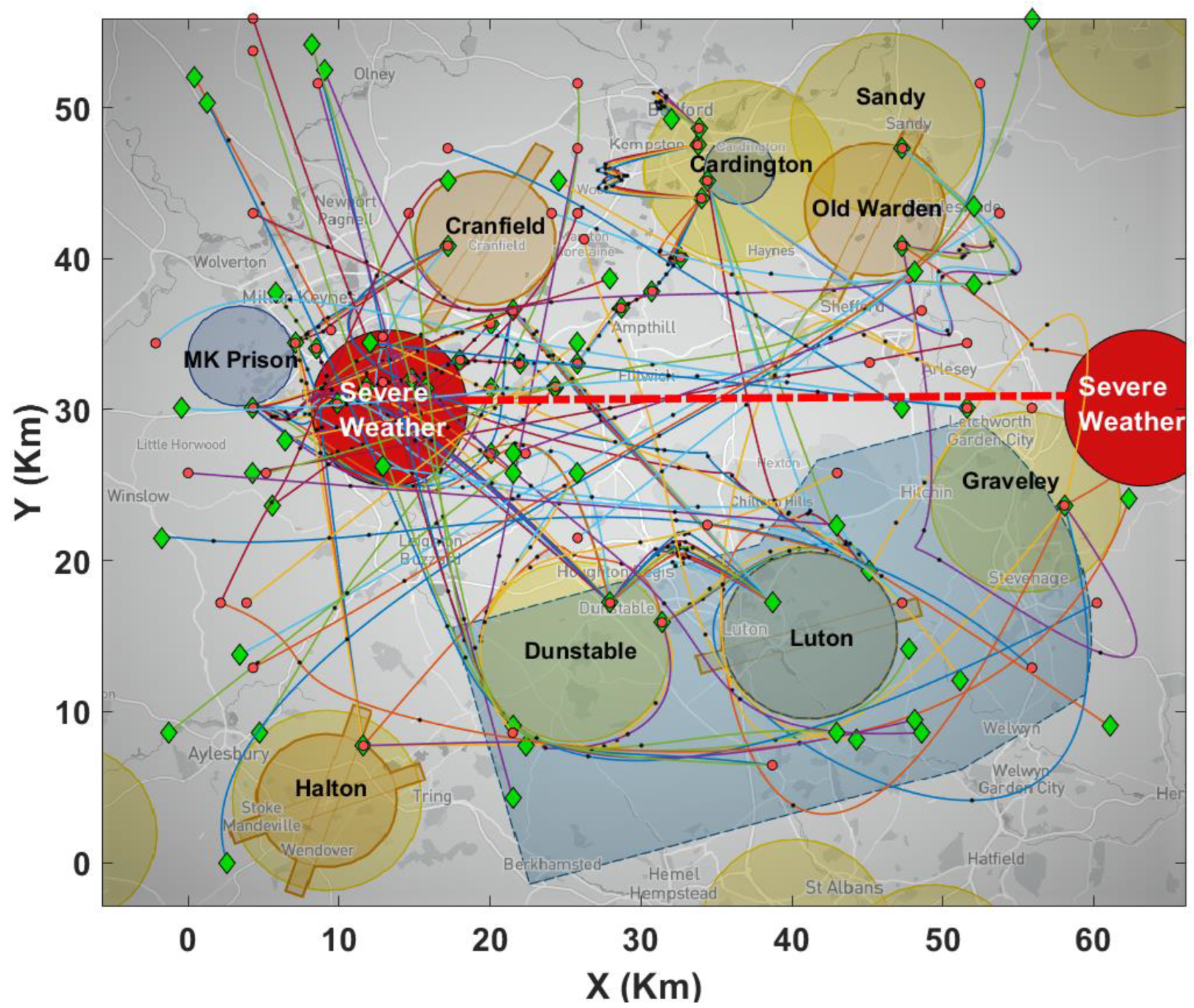
In order to assess and verify the method suggested by the present study, a simulation was conducted in the airspace over Bedfordshire, UK. The simulation identified areas where flight is potentially restricted, including four recreational zones (Cardington, Dunstable, Graveley, and Sandy—Yellow), four airfields (Cranfield, Halton, Luton, and Old Warren—Orange), and Milton Keynes Prison (Blue). In order to generate optimal pathways for a UAV service from starting point to delivery point, the simulation deployed an optimization algorithm based on PSO [70,71]. Validation of the proposed model was undertaken via a drone-delivery system: the latter was employed for package delivery, emergency fire surveillance operations, an inspection of the railway infrastructure with the use of UAVs, and the essential dispatch of COVID-19 test samples, with differing priority levels assigned to the operations in question.
To improve the validity of the scenarios, this study considered the influence of structural airspace configurations, such as static NFZs. During simulation hours, some of the recreational areas and airfields became dynamic in character, rendering some areas available and others unavailable. Moreover, research was undertaken regarding the influence of environmental factors (such as weather patterns).
The first assumption was (a) that a fleet of three UAVs (designated UAV1, UAV2, and UAV3) would be maintained by the Luton (Bedfordshire) National Health Service (NHS) hospital, and (b) that these would be used to deliver sample tests to a range of clinics within a defined distribution network. This UAV shuttle service would be organized on an hourly basis. The second assumption was that mail packages would be delivered to multiple post offices from the Luton central delivery office. Two vehicles would be deployed for this, namely, UAV4 and UAV5. The first would cover Cardington, Graveley, Old Warren, and Sandy, while the second would be allocated to cover Cranfield, Dunstable, Halton, and Milton Keynes Prison. The use of two UAVs in this manner was anticipated to improve customer satisfaction and minimize delivery times.
Camera-based surveillance operations were central to the rescue operations in question, which involve firefighting. The precise nature of the firefighting response was defined, at least partially, by the images and videos derived from the payload cameras. Only one UAV operation was considered within this scenario. As a base station for the relevant missions, we utilized the availability of UAV6 at Milton Keynes Prison Fire Station. We also implemented an inspection mission for railway tracks in the Bedfordshire area, with the aim of examining the technical condition of the railway infrastructure from Milton Keynes, via Bletchley, to Bedford central railway station. Two UAVs, namely, UAV7 and UAV8, were allocated for this inspection task. The former covered the track from Bedford rail station, via intermediate waypoints, to a railway station near Ridgmont, then back again to Bedford rail station for the next hour of inspection. Conversely, UAV8 was deployed to cover the track from Milton Keynes (MK) central rail station to Bletchley and back to MK rail station. Inspection took place on an hourly basis. In the scenarios we addressed, we considered where hobbyists might employ their own UAVs, in parallel with the missions outlined above. These trajectories were assumed to have one leg, with starting and finishing points determined at random. The missions themselves, and the simulation environment, are illustrated in Figure 2, while the plan and schedule for each mission are presented in Table 2.
In addition, the research assumed that UAVs would fly at constant speeds of 90 km/h and a fixed altitude of 100 m. Moreover, it was supposed that the sequence of clients to be served along flight routes would determine delivery times. A particular route was allocated to each UAV, with routes beginning and ending at the depot. If the vehicle followed an assigned route in its entirety and returned safely to the depot, the mission was deemed to be completed. Table 3 provides the technical parameters for the UAVs used during the simulation scenarios.
The present research addressed certain deconfliction strategies, with a view to overcoming any UAV conflict that may arise in different environmental scenarios [72]. There are three principal stages to the suggested rule-based, conflict-management model. The first stage, namely, strategic deconfliction, is applied when the time-of-flight plan is generated. This comprises two distinct methods—a filling service and pre-flight rerouting. Within this strategy, the key concern is to modify routes in order to avoid zones of conflict. The filling service confirms whether the modified flight route remains clear of other trajectories. The second stage, meanwhile, is that of pre-tactical deconfliction. This resolves conflict by means of a ground delay, and the goal is achieved by subjecting lower-priority UAVs, prior to departure, to ground delays of between two and three minutes. These ground delays will continue to be implemented until conflicts are resolved. If resolution is impossible, however, the Extended Flight Plan (EFPL) will be canceled. Hovering comprises stage three of the deconfliction model, and this is applied during flight. Until a conflict is resolved (or until landing, in the case of battery expiration), the UAV will hover at a waypoint that precedes the conflicted zone. Battery endurance will determine the length of time that this deconfliction process may continue, while obviously, hovering is not an option for fixed-wing UAVs.
The following simulation parameters were adopted:
  • Fixed positions: Starting and ending within this simulation, the start and end positions for the UAV missions were calibrated to imitate real emergency services and typical daily operations.
  • Levels of priority: A priority service level was allocated to each flight, ranging from Level 5 (lowest priority) to Level 1 (highest priority). The various levels are described below:
    • Fire surveillance and emergency services
    • Delivery of COVID-19 test samples to multiple clinics
    • Delivery of packages to assorted post offices
    • Scheduled railway track inspection missions
    • Random flights for hobbyists (single-leg missions)
  • Dynamic NFZs: Some of the recreational areas and airfields incorporated in the simulation were dynamic in character, at least at certain times. This dynamism was random, rendering some areas available and others unavailable throughout the simulation hours.
  • Random times of departure: For each one-hour simulation period, to make the exercise more realistic, the precise time of departure for each hobbyist’s UAV was placed randomly between one and ten minutes.
  • ‘Ambiguous’ weather: Varying weather conditions, including ‘severe’ and ‘adverse’, were addressed. This study [73] presented details regarding the implementation of weather effects.
  • Strategy for deconfliction: Within the simulation setting, ground delay was deployed as a deconflicting strategy.
To simulate more complex dynamic airspace, this study simulated a multi-mission scenario between 9:00 am to 12:00 pm for the Bedfordshire area. This study considered the five missions mentioned earlier in this scenario.
Three different sub-scenarios were created for each hour of simulation covering the above missions:
1.
First simulation scenario: This simulation ran between 9:00 am and 10:00 am. In this scenario, all nine NFZs were static without any dynamic obstacles and weather constraints. As a result of this constraint, no UAV could fly over them during this hour. Moreover, this scenario was conducted by 100 UAV trajectories. The railway track inspection mission by UAVs was not considered in this scenario.
2.
Second simulation scenario: This simulation ran between 10:00 am and 11:00 am. The difference between this and the first scenario was that more complexity was added to the Bedfordshire airspace by considering Railway Infrastructure Monitoring operations and increasing the number of UAV trajectories to 150. The effects of adverse rain and wind were considered in this scenario.
3.
Third simulation scenario: 200 UAVs’ trajectories in airspace were considered in this simulation that ran between 11:00 am and 12:00 pm. In this scenario, airfields were dynamic, while all four recreational areas and the prison were kept static. Among the four airfields, Luton and Cranfield were available, and therefore, recreational users of UAVs could fly over Luton and Cranfield at some points. This scenario also incorporated severe weather effects. The scheduled inspections of railway tracks by UAV operations were considered in this scenario.
For simplicity, the figure of one of these scenarios is presented in Figure 3.

3.2. UAVs States Formulation

With a view to testing the predictive capacity of the proposed model vis-à-vis traffic complexity, the present study used a dataset of simulated historical trajectories that were generated in the previous section. A trajectory is defined as a sequence of UAV states. Each UAV state consisted of the following five elements: longitude ( x ), latitude ( y ), timestamps ( z ), velocity ( V ), and heading ( H A ) for each UAV.
These UAV states were used to train datasets to predict UAV traffic flow through the airspace. To predict the airspace flow patterns, UAVs dynamic variables sampled at 10 sec intervals were used to formulate state vector, which showed the sequential behavior of the UAV. Each UAV’s longitude and latitude coordinates at all time instances were generated based on the waypoints of the UAV during the PSO-based simulation scenario. The heading angle and velocity of each UAV can be evaluated using longitudinal and lateral coordinates at each timestamp. Velocity was calculated as:
v k = x k x k 1 + y k y k 1 z k z k 1
where k represents current time instant and x and y represent longitudinal and lateral coordinates, respectively. Timestamp has been represented by z in (1). Similarly, heading angle is evaluated using the change of the UAV’s trajectory in the x and y coordinate system. Heading angle ( H A ) can be stated as:
H A k = t a n 1 y k + 1 y k x k + 1 x k
Discretized trajectories can be used to evaluate UAV speed, heading angle, and congestion matrices at each time instant. State vector for a certain UAV at a certain time instant can be given as:
State = [Timestamp, Longitude, Latitude, Velocity, Heading Angle]

3.3. Computation of Complexity Metric: Spatio-Temporal Correlation

The frequency of aircraft passing through a given region, over a certain period of time, is known as air traffic density, or congestion [74]. Higher air traffic congestion heightens the possibility of air traffic incidents, and thus necessitates rigorous monitoring [75]. The increase in complexity can negatively impact controller’s decision-making abilities, resulting in increased errors [76]. Thus, so-called “hot spots” of air traffic congestion necessitate scrutiny from controllers to determine whether conflict avoidance or modification is required for any planned trajectories. An important aspect in this regard is the measurement of air traffic complexity. The literature provides several metrics, developed and implemented for the purpose of measuring air traffic complexity. These include convergence and geometric metrics [31], a clusters metric [77], the Grassmannian metric [78], and finally, the König metric [79]. Whilst these metrics have proven effective in basic scenarios, they are nonetheless unsuitable for complex and/or large-scale applications. The methodologies also fail to take proper account of spatiotemporal data [80]. The present study sought to overcome these difficulties via the adoption of an air traffic complexity metric centered upon the Linear Dynamical System (LDS). Via analyses of traffic structures and airspace geometries, numerous studies have analyzed traffic structures and airspace geometrics to demonstrate the efficacy of LDS as an intrinsic complexity measurement [30,31,32]. Moreover, LDS is appropriate for use as an estimation metric for local disorder and the interaction of trajectory sets within the UTM system. Its suitability derives from its efficiency and relative simplicity, and the fact that it evinces mathematically predictable behavior.
The intrinsic complexity metric deployed in the current study is adapted from a previously published linear dynamic system model applied for ATM domain [29]. The metric identifies a complexity parameter in the vicinity of a UAV for a specified time. Flights that are likely to engage with the reference flight are accommodated via a filter. In this work, a safe distance of 50 m was maintained to avoid any conflict (thus, a drone 50 m from the reference vehicle was omitted from the metric computation as it would not interfere) [81]. The suggested complexity metric was specifically designed to capture, within a reference airspace window, the dynamic behavior of nearby drones. In order to identify the geometric behavior of the trajectories, the velocity of the UAVs ( U ˙ ) was connected to the position of the UAVs (U) via deployment of the following linear dynamical system [31]:
Let us define matrices P and V as:
P = x 1 x n y 1 y n z 1 z n a n d     V = V x 1 V x n V y 1 V y n V z 1 V z n
where x 1 ,   y 1 ,   and   z 1 denote the spatial-temporal coordinates, and V x 1 ,   V y 1 ,   and   V z 1 denote the velocities of the first drone in the vicinity of the reference UAV. The matrix A U and the vector b are determined with least mean squares:
m i n A , b V A U P + b 2
The dynamical system defined by A U and b is the tightest approximation of the current air traffic situation (positions and velocities) by a linear dynamical system. A convergence behavior corresponds to trajectories getting closer to each other, and this increasing proximity is itself associated with heightened complexity. The eigenvalues of the state-transition matrix characterize the behavior of the linear dynamical system and thus can be used to quantify the geometric properties of the considered traffic situation. More precisely, eigenvalues with positive real parts correspond to divergence behavior, while eigenvalues with negative real parts correspond to convergence behavior (Figure 4). The complexity is related to convergence behavior since convergence increases the risk of collisions. Consequently, complexity in the vicinity of the reference UAV is defined as follows:
c A U   = R e λ A U   < 0 R e λ A U    
The metric c A U is therefore a parameter of the magnitude of the divergence or convergence activity of the dynamic system.

3.4. Implementation of Encoder-Decoder LSTM Model

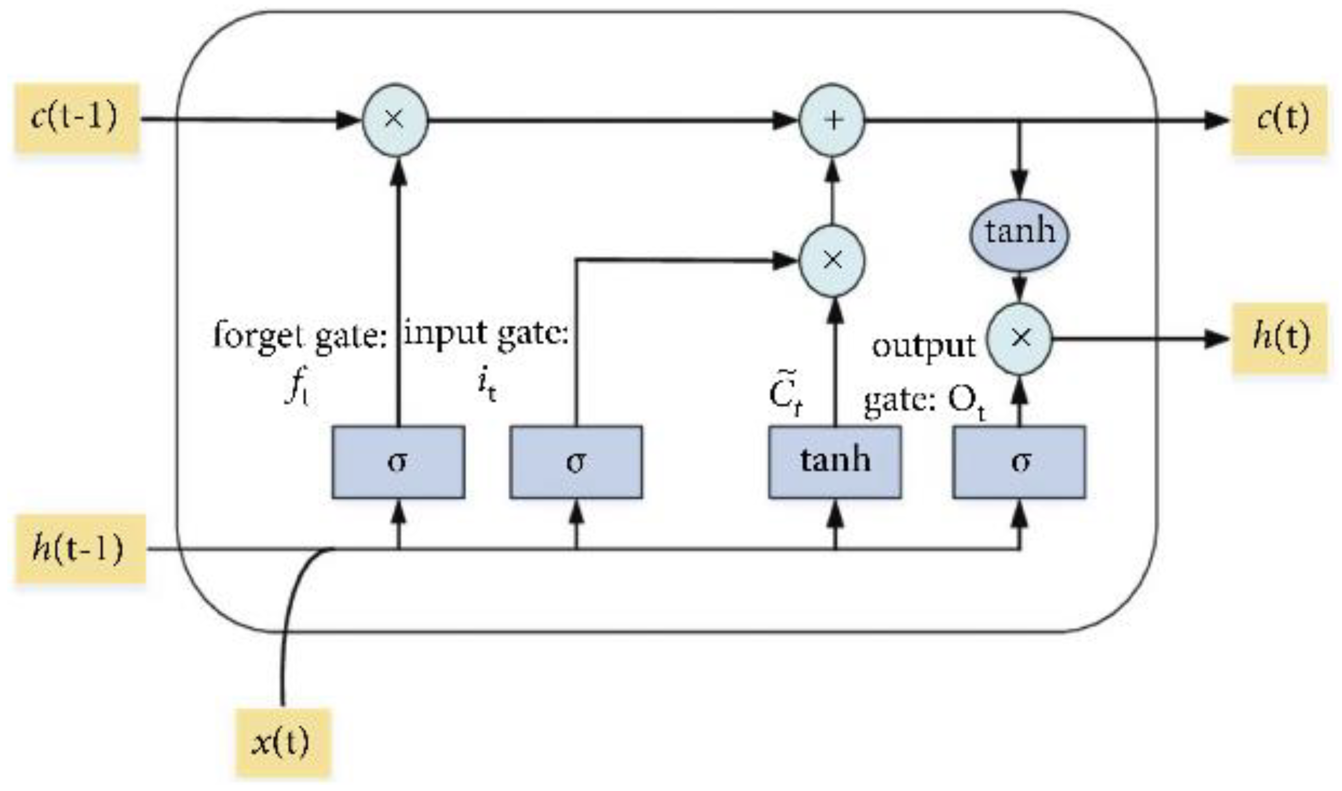
As set out in the introduction, this study aimed to improve the accuracy of complexity prediction in congested airspace. In order to extract complex patterns from time series data, an encoder-decoder architecture was used that relies on LSTM layers and a one-dimensional (1D) convolutional layer. In the context of learning long-term dependencies, challenges are encountered by the empirical RNN layer if the linear dimensions of the sequence are relatively large—an issue designated as the ‘vanishing-gradient problem’ [48]. Various RNN layer configurations with long-term memory, e.g., LSTM, have been deployed in an effort to resolve this matter [49]. LSTM comprises four regulatory gates, namely, input, forget, cell, and output, in addition to hidden units. Figure 5 provides the overall configuration for a single LSTM block, while the mathematical description is as follows:
I t = f W i x x t + W i h h t 1 + W i c C t 1 + b i   F t = f W f x x t + W f h h t 1 + W f c C t 1 + b i f   C t = F t C t 1 + I t g W c x x t + W c h h t 1 + b c   O t = f W o x x t + W o h h t 1 + W o c C t + b o   h t = O t g C t  
where the activations of the input, forget, cell and output gates are denoted, respectively, by I t , F t , C t and O t , and h t represents the hidden unit. The forecasting time step is represented by the t superscript. The weights matrices are denoted by W, and the bias vectors by b, with corresponding subscripts.
Because input and output sequences may have different lengths, it is difficult to resolve certain problems related to sequence-to-sequence prediction. The encoder-decoder LSTM has been designed to address such problems. The input sequence is encoded into a fixed-length vector by the first model, while the fixed-length vector is decoded by the second model, which also generates an output for the forecast sequence [58]. This configuration is unique due to the use of a fixed dimensional intrinsic representation in the center of the model termed ‘sequence embedding’ [83]. Both the encoder and decoder may be described as RNNs, i.e., LSTMS.
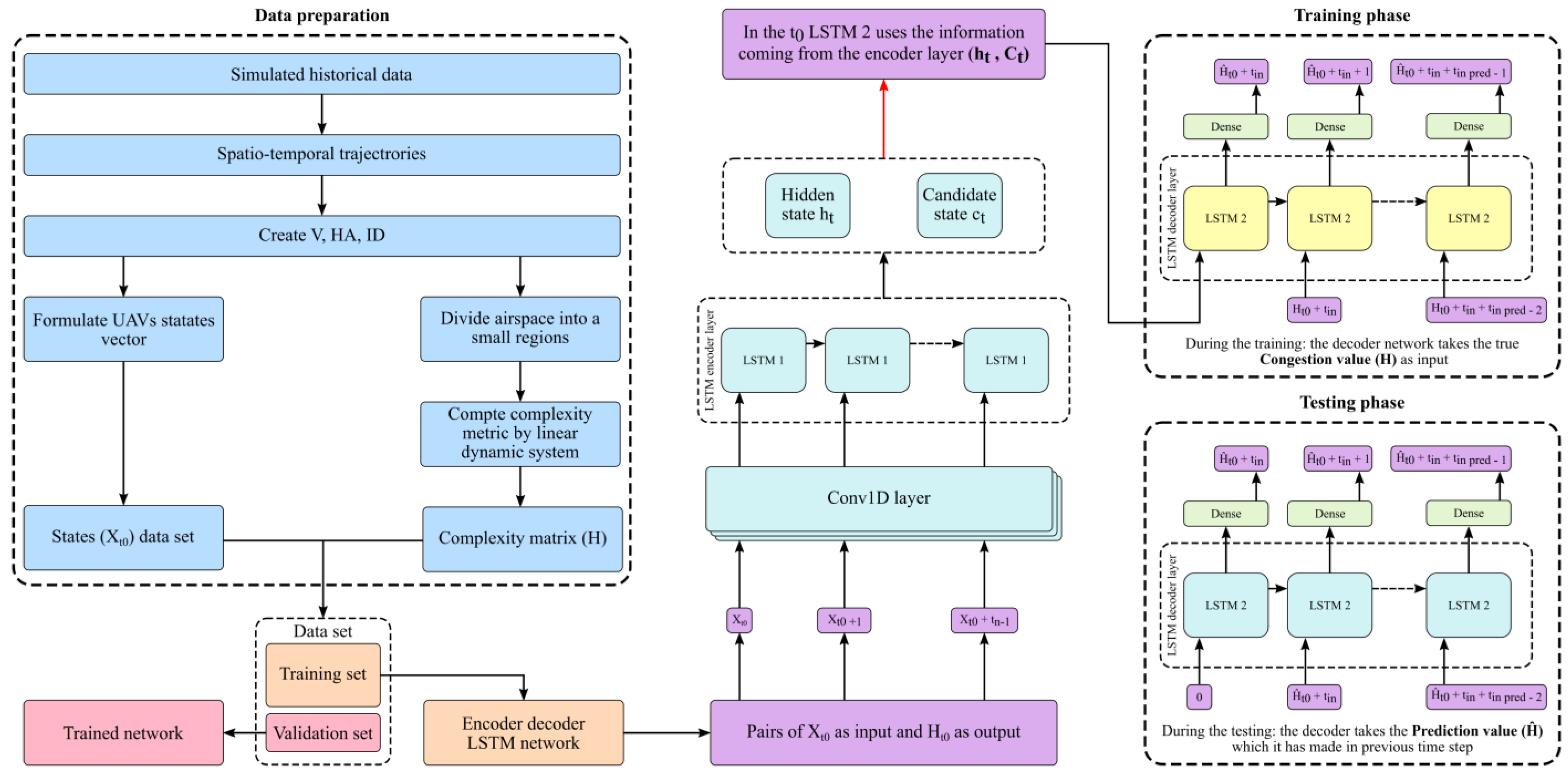
Figure 6 presents the structural diagram for the model proposed in this study. The final dataset is composed of various sizes of simulated trajectories that have developed based on three scenarios outlined in the experiment design and data generation section. In all three situations, the data points of each trajectory differ based on the time of flight. The sets of data points in 100 UAV’s first scenario reached 132,148, whilst for 150 UAV scenarios, a total of 181,505 sets of data points were recorded. During the third hour of simulation where 200 UAVs were considered, the dataset contained 252,129 data points. The proposed model was trained on 90% of the dataset, after which it was tested on the remaining 10%.
At a given time t ,   X is used to represent the state vector of the i th trajectory. Subsequently, X t is defined as the concatenation of all state vectors X , which applies to all UAV trajectories in the airspace. The prediction target is complexity matrix H t . In order to identify neighboring UAVs in such a way that each cube corresponded to an element of H t , the airspace was divided into small cubes. The complexity metric was then computed for all UAVs currently in each cube. Moreover, t in represents the duration of the observation window (i.e., the number of time steps observed before making predictions), whilst t pred represents the prediction horizon (i.e., the number of time steps that need to be predicted). For the encoder network, the number of time steps was maintained at t in = 36. This corresponds to three minutes, or 180 s, since one time step comprises five seconds. In other words, to generate its prediction, the model can access the last three minutes of traffic. The decoder network predicts a sequence set to t pred = 36, and this correlates with the complexity values of the next three minutes.
The dataset was composed of pairs of sequences ( X t 0   ,   X t 0 + 1   , . X t 0 + t i n 1   ) ,   ( H t 0 + t in ,   H t 0 + 1   , . H t 0 + t p r e d 1   ) . For complexity prediction purposes, an encoder-decoder LSTM model was employed. The encoder network used a sequence of UAV states ( X t 0   X t 0 + t i n 1   ) to output an encoding vector. The decoder network then uses the encoding vector and the complexity matrix predicted at the last timestep H ^ t 1 to predict the next complexity matrix H ^ t .
The first layers of the encoder network can be designated a ‘single-dimension convolutional layer’. These layers process the input sequence corresponding to the UAV states. Different f filters comprise each layer, and these filters further encompass a kernel of learnable value parameters, with the dimension d * m , where m and d indicate the input sequence, and kernel width, respectively. The result of the input sequence, as it is relating to the distance, is aggregated by the individual filters, while each output series element comprises data from several serial time increments. This can be represented as follows:
y i j = k = d d l w k l j x i + k , l   ,
where y i j denotes the j t h vector element of the i t h sequence term, and x k l signifies the l t h vector element of the k t h sequence term of the input. Meanwhile, w j k l represents the k t h weight of the kernel of the j t h filter, as related to the l t h dimension of the input sequence; finally, Φ denotes an activation function. The implementation of convolution operations occurs exclusively along the time dimension of the input sequence hence, the use of the term ‘one-dimensional’ (1D). The convolutional layers were deployed to identify dependencies within a short time period. Thus, the processing of the LSTM layer is facilitated by incorporating dynamical information from the preceding and subsequent time steps. Without the convolutional layer, conversely, the LSTM layers would merely be capable of processing each of the time intervals consecutively, absent any data from subsequent time increments. The parameters of the proposed model are presented in Table 4 below.

3.5. Model Training

The objective of our supervised learning model is to provide accurate congestion forecasting in UTM systems. For the model’s objective to be realized, it is necessary to construct a training set by deploying training input/output pairings. The input vector X t comprised sequences of UAV states, duly matched with complexity value sequences for the airspace as a whole. To generate the training outputs, for each time increment t , the complexity matrix H t is defined as an n × n .
The hidden states of the final LSTM layer form the encoding vector—no other encoder data will be supplied to the decoder network; the decoder network is composed of several LSTM layers whose hidden states are initialized with the encoding vector. These LSTM layers are followed by several dense layers. The output from these layers is a vector that had an n 2 dimension, equivalent to the matrix of the complexity metric.
The decoder input is formed by two elements, i.e., the encoder output, and the previously predicted or decoded output sequence term. During the training, the decoder network is trained by a method referred to as ‘Teacher forcing’ [84,85]. This method consists of using the output predicted at the previous time step as input for the decoder network. The prediction identified at the preceding time interval is thus accounted for within the inference mechanism. The list of model hyperparameters is shown in Table 5.
The root mean square error (RMSE) was used to assess the performance of each selected approach, and served as the estimation criterion for the performance of the proposed model. The following expresses the RMSE, which denotes the loss function:
RMSE = 1 N k = 1 N C a c C p r 2 ,
where N denotes the total number of airspace (x, y) coordinates, C a c signifies actual congestion volumes at any specific point k , and finally, C p r represents the forecast congestion at the precise (x, y) coordinate. Since differences between forecast and actual values are ‘less’, higher predictive accuracy is reflected by a lower RMSE value.

4. Results and Discussion

For the scenarios described in Section 3.1, the performance results of the proposed architecture are presented below. Ideal mission plans are disrupted by the three scenarios, via the interpolation of dynamic random factors, including uncertain weather, recreational areas, and airfields. A comprehensive comparative analysis was deployed to assess the performance of the suggested forecasting model.

4.1. Prediction Result

4.1.1. First Scenario Simulation

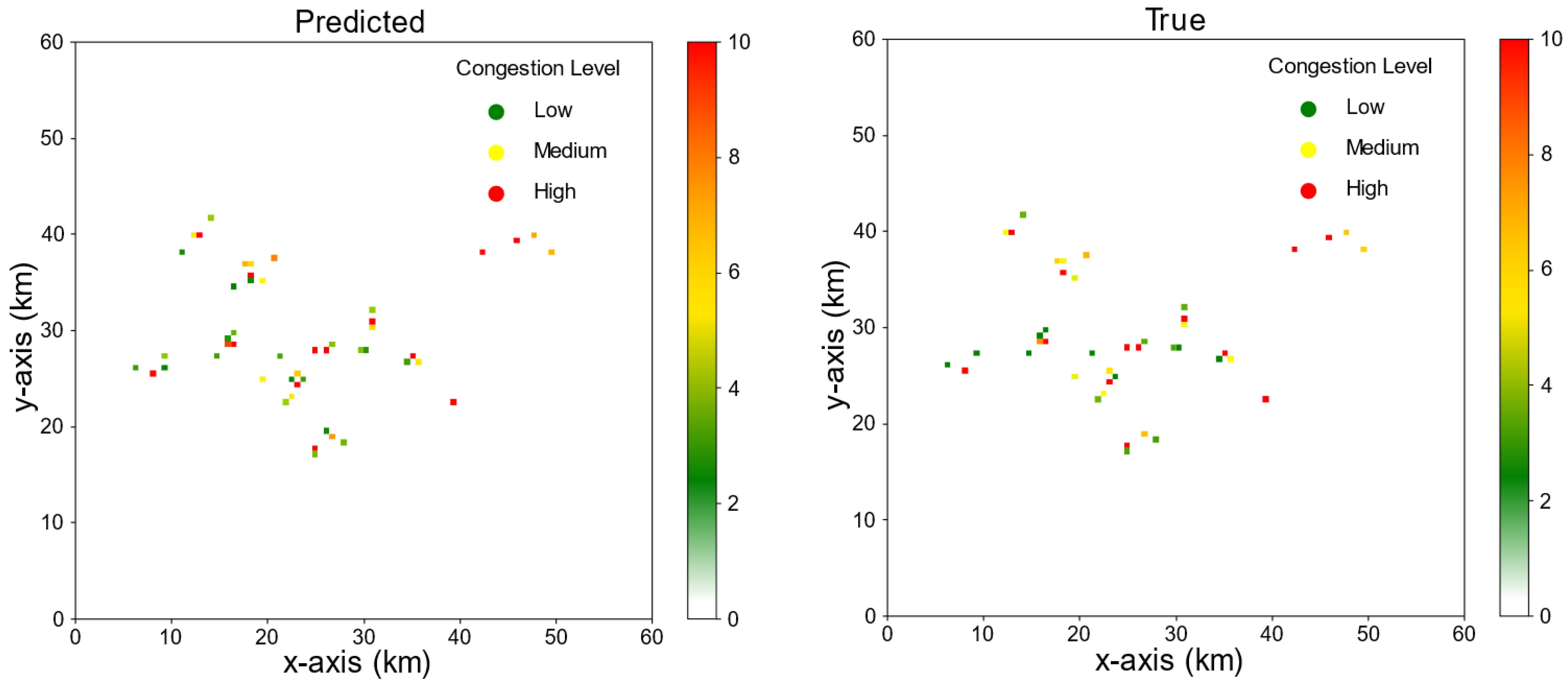
This case postulated a scenario of 100 UAVs with an NFZ but no adverse weather conditions; the objective was to evaluate airspace congestion. Figure 7 presents a heat map for the scenario congestion matrices, and it addresses the Bedfordshire airspace congestion caused by UAVs in the neighborhood. The airspace was analyzed in order to predict the density of the UAV trajectories at each square km area. The low to high densities of UAVs per square km are represented by red and green, signifying the highest and lowest complexity, respectively.
The figure illustrates that most of the highly complex regions in the future timestamp were captured by the proposed model. The RMSE value of the prediction was employed to evaluate the performance of the LSTM trained architecture. RMSE reached a value of 0.1662 for this scenario, indicating high model accuracy. Furthermore, it is evident from the residual plot (Figure 8) that predicted complexity was very close to true complexity, with very few wrong detections during the prediction process. Moreover, although most of the congestion areas were captured, the regions with high complexity depicted a small difference in magnitude between true and predicted complexity.
Statistical analysis of the actual, predicted, and residual complexity figures was completed to present the above information in greater depth. In this regard, the analysis normalized the complexity values for each complexity point between 0–100 whilst also taking into account the maximum complexity points for all true, predicted, and residual vectors. The percentages for the complexity figures were then plotted against the trajectory points. The largest value of residual complexity percentage represents the maximum dissimilarity between empirical truth and predicted complexity. Furthermore, the number of residual complexity points below an acceptable threshold were counted to provide a means of evaluating the performance of our proposed methodology. The statistical analysis of the residual complexity for scenario 1 is presented in Figure 9 below.
The statistical analysis of percentage complexity for scenario 1 showed that the maximum dissimilarity in complexity between ground truth and prediction using LSTM was 12%. Furthermore, 83% of complexity points had less than 5% residual complexity, which indicates better prediction performance. The peak residual complexity values correspond to the regions with the highest complexity trends.

4.1.2. Second Scenario Simulation

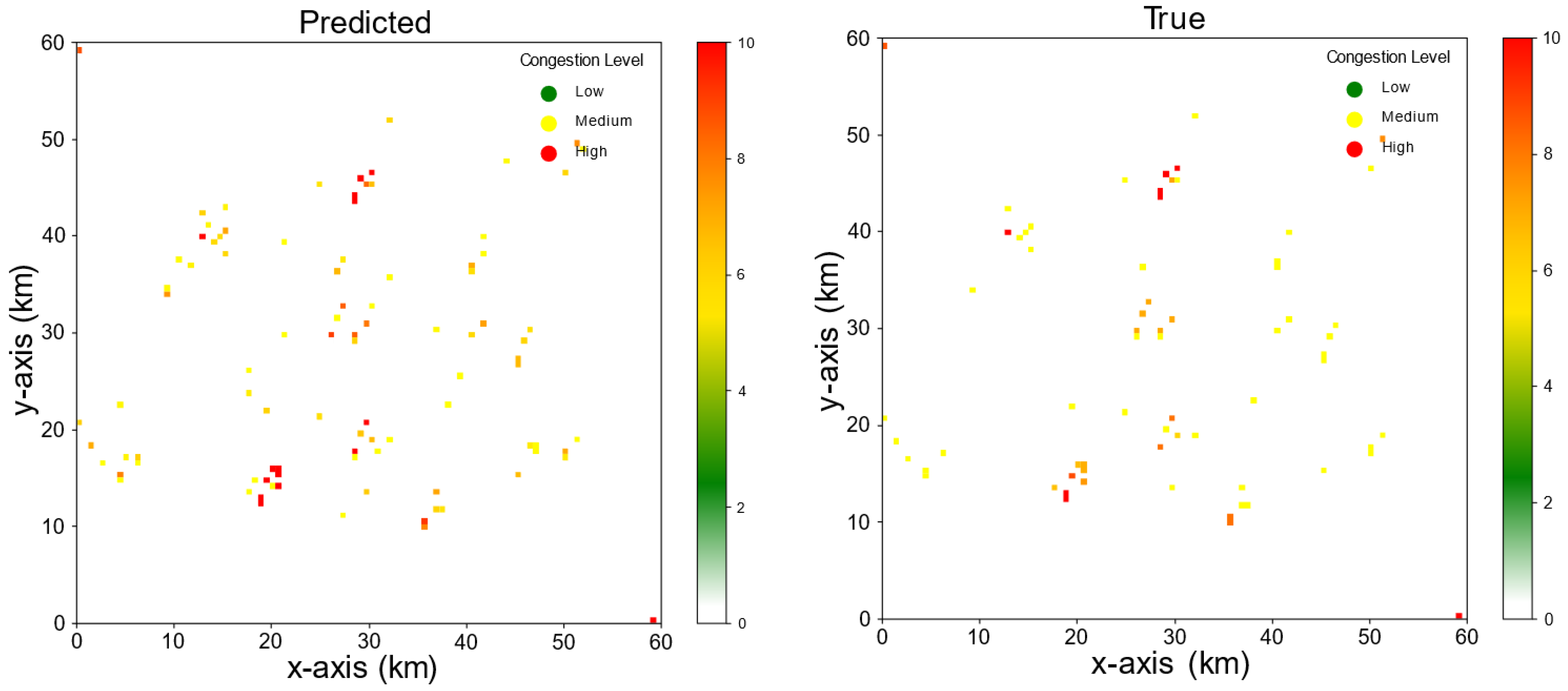
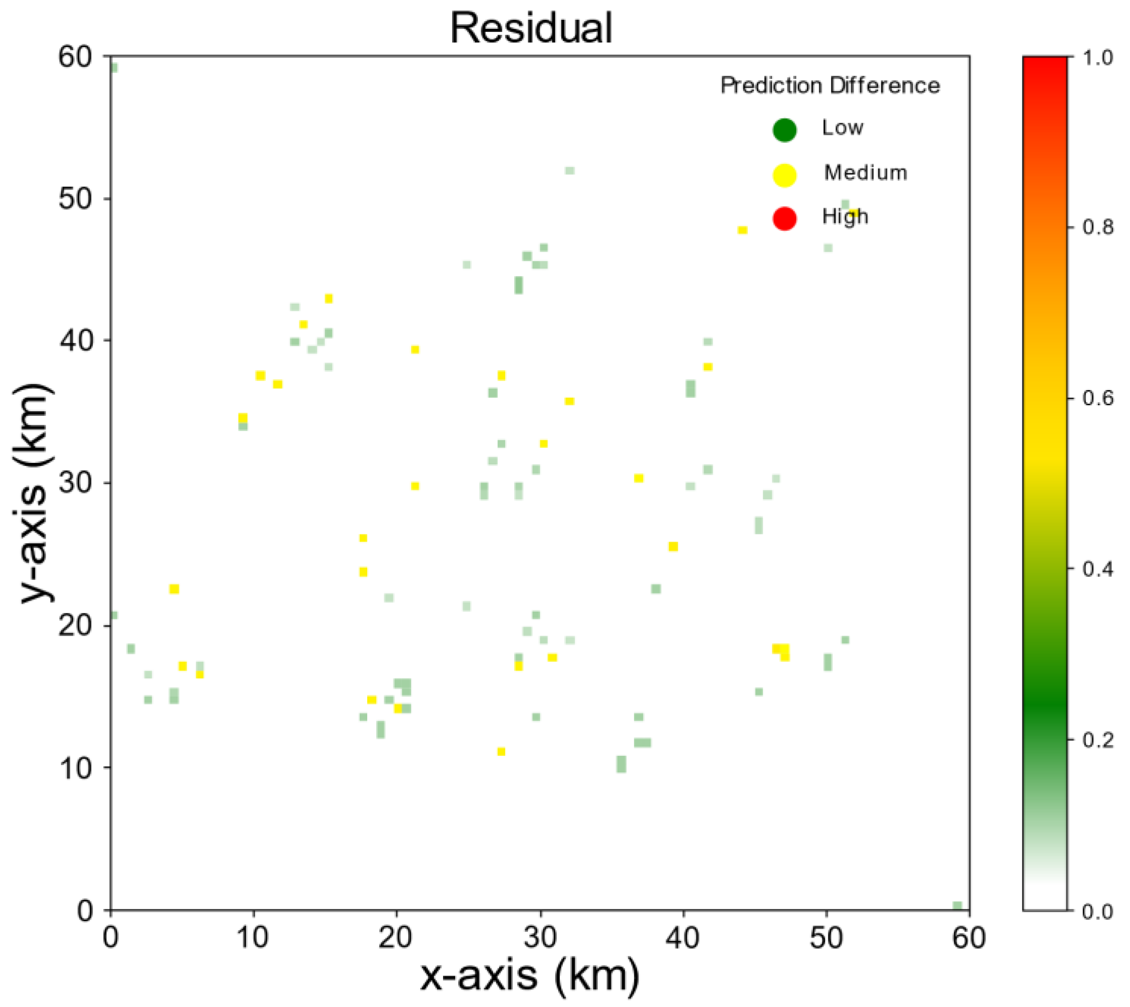
In scenario 2, the putative complexity of the Bedfordshire airspace environment was increased. The number of UAVs increased to reach 150 by considering railway infrastructure monitoring operations, dynamic recreational areas, and uncertain weather with adverse wind and rain. Figure 10 comprises the resulting congestion heatmap. As the heatmap demonstrates, by observing the speed, congestion areas, and dynamic behavior of the UAVs, the encoder-decoder model captured major complexities within the airspace. The performance of this model may be quantified via the RMSE (0.2852) for training and validation at each epoch. Similarly, Figure 11 represents the residuals of the predicted values in relation to the actual ones. Density increases in line with increases in the number of UAVs, as the figure clearly indicates; this phenomenon stems mainly from significant fluctuations in observable traffic patterns. Increasing density, furthermore, is driven to a large extent by dynamic weather constraints. The residual in the previous scenario was calculated to observe the non-detection, wrong detection, and detection differences in the true and predicter airspace complexity values. Additionally, the residual plot shows a very small difference between the actual and true complexity heat maps.
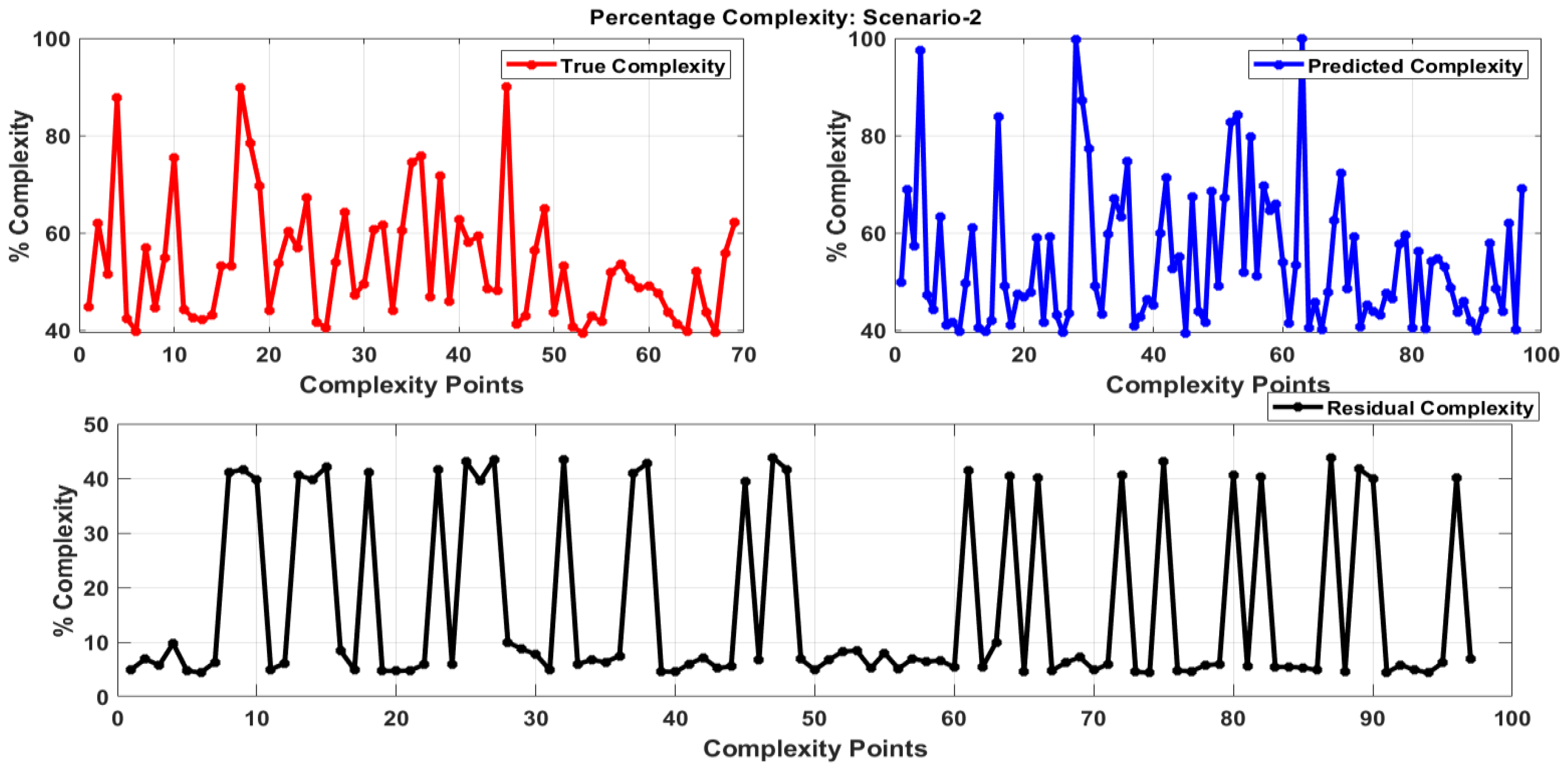
Moreover, the residual analysis in Figure 12 demonstrates that the maximum dissimilarity of complexity between ground truth and prediction using LSTM was 43%. Moreover, 70% of complexity points had less than 10% residual complexity, indicating better prediction performance. The peak residual complexity values correspond to regions with maximum complexity trends.

4.1.3. Third Scenario Simulation

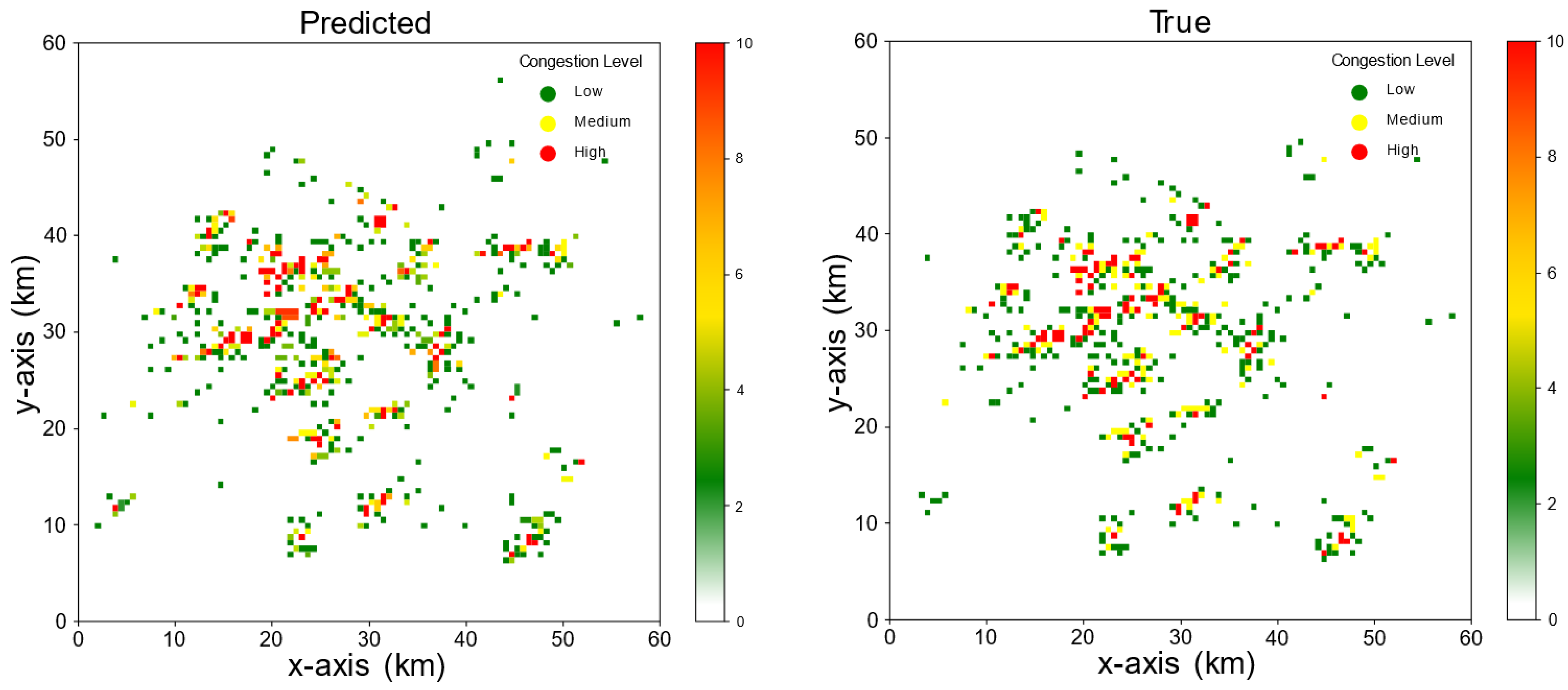
Altogether, 200 UAV flights in airspace were considered in this scenario, including the scheduled inspections of railway tracks by UAV operations. Although the airfields were dynamic, all four recreational areas and the prison remained static. Furthermore, severe weather effects were considered during scenario 3. Figure 13 provides the resulting congestion heatmap, indicating that the temporal and spatial transition patterns of air traffic flight flow were indeed learned by the proposed model. Future air traffic flows may be predicted since the primary characteristics of these flows are captured. The third scenario generated an RMSE value of (0.6021), and the prediction from the trained model architecture is sufficiently close to the true congestion value. This indicates that the proposed ATFP architecture performs optimally.
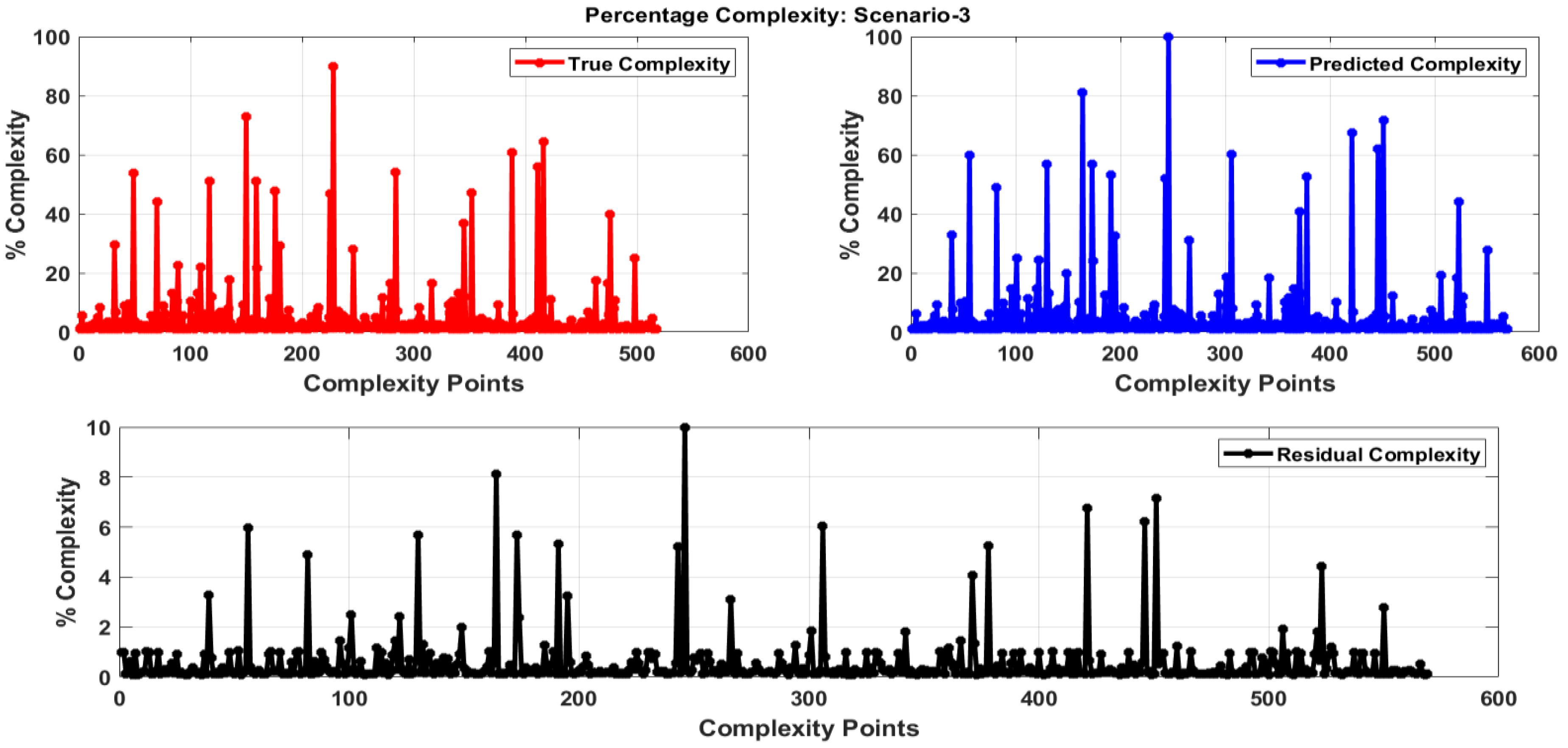
A residual plot is presented in Figure 14 to highlight the accuracy of predictions made by the proposed LSTM network. Given the higher density of UAVs in airspace, the prediction also depreciated, which is evident from the absolute difference between true and predicted airspace congestion. Moreover, given the incidence of incorrect detection, some high congestion spots were visible in the residual plot. Most of the predicted airspace complexity values were correct, which is evident from the RMSE between true and predicted airspace complexity. It was observed from Figure 15 that the maximum dissimilarity of complexity between ground truth and prediction using LSTM was 10%. Moreover, 97% of complexity points had less than 5% of residual complexity, which indicates optimal prediction performance. The peak residual complexity values correspond to regions with maximum complexity trends.

4.2. Comparison between Existing Approaches and the Proposed Model

As noted earlier, the predictive quality of the proposed model has been compared with two other predictive methods, as described in Section 2. The three scenarios were used to assess the performance of each approach. For analytical comparison with the proposed model, the first selected architecture was a shallow NN-based model (with dense network connections) as described in [87]. The second was a regression architecture-based Nonlinear Auto Regression, with External input (NARX) model, as described in [36]. Calculation of the RMSE was used to assess the performance of each selected approach, and RMSE served as the estimation criterion for the performance of the proposed model. The predictive quality of the proposed LSTM, meanwhile, was evaluated via a comparison of the descriptive statistic values of the predictions with the actual values. Between the actual and predicted values, the descriptive statistics were as follows:
Mean   μ = 1 N k = 1 N C ac C pr ,
Standard   deviation   δ = 1 N k = 1 N C ac C pr   μ 2 ,
AMPE   η = 1 N k = 1 N C ac C pr C ac × 100 %   ,
where N signifies the overall number of airspace trajectories (x, y). Meanwhile, C a c denotes true congestion values, as identified by using the dynamic linear UAV model illustrated in Section 3.4. C p r signifies the forecast congestion at the particular airspace coordinates (x, y), based on the LSTM encoder-decoder architecture. The degree to which the predicted point deviates from the data mean is assessed via the standard deviation. In order to present the total deviation of the predicted values from the mean value, every predicted point variation is measured and summarized. The prediction accuracy of the model, in percentage terms, is measured via the absolute mean percentage error (AMPE). Figure 16 illustrates the descriptive statistics and RMSE calculations for the actual and predicted values.
As the graphs indicate, the LSTM model has the smallest RMSE value of all the indices. This confirms the hypothesis that combining the advantages and features of various algorithms and models (i.e., 1D convolutional and LSTM) affords superior problem resolution [88]. Clearly, this also applies to the problem of ATFP in Bedfordshire considered in this study. The results of the comparison demonstrate a superior performance of the deep learning model compared to the existing approach. Toolbox availability renders Shallow and Regression networks easy to construct, but these fail to capture the complicated relationship between complexity metrics and states.
The superiority of the encoder-decoder LSTM predictive model stems not merely from its predictive capacity, but also from its input and output structures, which facilitate airspace complexity predictions with consecutive time steps. When airspace congestion is presented via a temporal and spatial scale, airspace complexity can be assessed more intuitively. UTM operators may thus look to the future with a sense of how airspace complexity will vary with regard to different time slots. The proposed model shows superior predictive performance in comparison with the other approaches, because both temporal and spatial dependencies are modelled. The three scenarios cited above also simulate differing meteorological ambiguities. Only the influence of historical data (temporal, but not spatial correlations) is reflected in the regression model. The latter is thus notably dependent on the magnitude of the data and the look-ahead horizon. Unexpected variations in air traffic flow, weather conditions, and flow patterns may also impact the performance of the regression model. Air traffic complexity is more effectively captured by the shallow NN (used in conjunction with a dense network connection). The spatial coordinates of airspace complexity could be predicted more accurately than with the regression model. Nonetheless, the proposed model also demonstrates superior performance in comparison with the shallow NN.

4.3. Comparison between Existing Approaches and the Proposed Model: Performance vs. Time

The prediction performance parameters narrated above have been plotted against prediction time in order to temporally and spatially visualize the efficiency of the proposed methodology. Figure 17 shows that complexity prediction performance parameters (such as RMSE and AMPE have much smaller values in the proposed model than other already-proven prediction approaches (such as shallow NN and regression model (NARX)). It can also be seen that the AMPE grows much faster for adverse wind, rain, and extreme weather front scenarios between 10:00 AM to 12:00 PM.
This study analyzed the mean values of the computation time and performance parameters across the temporal domain between 9:00 AM and 12:00 PM (scenario 1 to scenario 3). This is presented in the bar chart displayed in Figure 17. Additionally, the mean value analysis shows that shallow NN had steady performance on the computation side with an average time of 2.4 s, although it displayed poor statistical performance with RMSE:3.1 and AMPE:9.0. The regression had slightly longer average computation times of 3.8 s and worse complexity prediction statistics with RMSE:7.0 and AMPE:13.1. The proposed model had optimal performance statistics with RMSE: 0.4 and AMPE: 3.4, although it has poor or large computation overheads with average computation timings at 100.3 s. Thus, the proposed methodology shows fewer RMSE and AMPE errors with improved performance at the cost of increased prediction times. On the other hand, Shallow NN and regression methods seem to have vast prediction errors but fewer computation overheads.

5. Comparison between Existing Approaches and the Proposed Model: Computation Speed

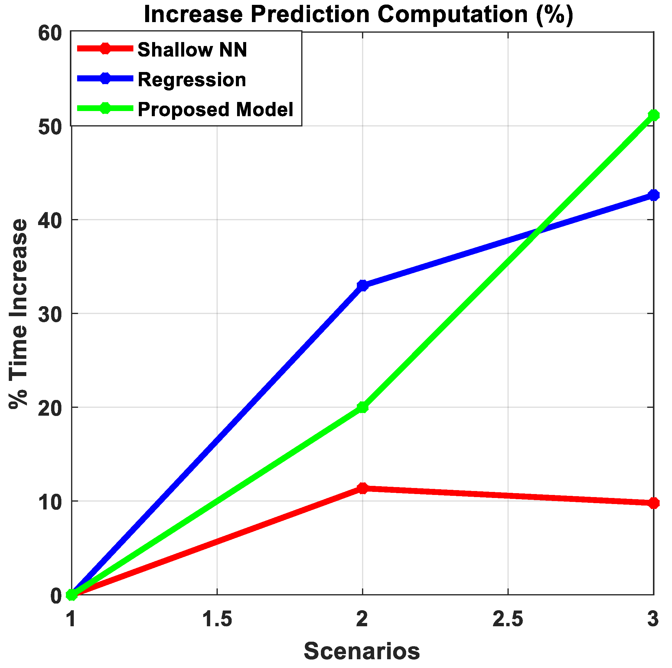
This study also evaluated the real-time implementation feasibility and computational performance benchmark of the proposed LSTM prediction architecture. This study used the prediction results on Intel(R) Core (TM) i7-8550U CPU @ 1.80GHz with 16 GB RAM. The computation time results were obtained for all three scenarios’ data and compared to the NN model, regression model, and the proposed LSTM method. A comparative analysis of prediction time was carried out between the proposed and other studied architectures. The evaluated prediction times for all of the architectures are presented in Figure 18. The analysis also measured the percentage increase in computation times across all three scenarios and covered both temporal and environmental aspects. This analysis is presented in Figure 19.
It is also evident from Figure 19 that the prediction times for shallow NN-based prediction steadily increases by 10% to 11%. On the other hand, the increase in prediction times for regression and LSTM methods was even more significant at 32% to 42%, and 20% to 51%, respectively. Thus, it is clear that the percentage increase of prediction times remains steady for shallow NN but increases faster for regression and LSTM-based prediction methods between 9:00 AM to 12:00 PM from scenario 1 to scenario 3.
It is deduced from the above results that the prediction time of the shallow and NARX networks is less than the proposed LSTM architecture. However, prediction times can be further reduced by increasing the computational effort and employing larger computational machines.

6. Conclusions and Future Work

There is a clear need for accurate congestion forecasting in UTM systems. This research study proposes a model to predict air traffic congestion using existing machine learning techniques and adapted complexity metrics based on a linear dynamic system. In contrast to previous studies [23] that have assumed a static environment, or have deployed a grid mission network model (as UAS traverses a region along a structured grid) [89], the proposed model was validated using a drone delivery system scenario which in turn addresses uncertainties generated by adverse weather, as well as dynamic and static obstacles. The present study contributes to the limited research on the prediction of air traffic flow for UTM systems, addressing the limitation that the existing literature covers either trajectory prediction [90,91] or conflict detection and resolution [92,93]. Deployment of the model aims to address issues related to UAV traffic management (e.g., congestion). In existing works [22,23], the CNN model has been employed to predict density in an urban area. Nonetheless, one of the major disadvantages of CNNs is the excessive cost of computation [94,95]. The present study proposes a DL model comprising LSTM and 1D-CNNs. This will have the dual benefit of enhancing deep neural network accuracy and saving time.
Based on complexity prediction graphs reflecting air traffic hotspots, the proposed model permits UTM operators to reconfigure and regulate UAV paths. It may be employed to recommend suitable conflict-avoidance trajectories through the manipulation of ground delay, speed, or heading, while also allowing congestion in predicted UAV-traffic hotspots to be reduced. By forecasting congestion areas in advance, and by facilitating suitable actions to prevent their emergence, the proposed model lightens the workload of air traffic controllers.
Severe weather, airspace restrictions arising from emergency operations, and potential collisions with both dynamic and static objects, all generate uncertainty within the UTM operational environment. In consequence, the traditional air traffic control paradigm makes it impossible for air traffic controllers to ensure the safety and efficiency of operations. It is, therefore, of great importance that a new decision support system (DSS) be designed as soon as possible, and specifically, one attuned to the needs of integrated manned/UAS Traffic Management. It is technically possible to construct highly automated UTM systems that deploy artificial intelligence (AI) algorithms. Nonetheless, intelligent algorithms typically evince opacity, and are deficient in transparency and inexplicability, which restricts their practical application [96]. With these challenges in mind, future work by this team will involve recommendations for a decision support system to aid UTM controllers. The system will help the latter predict the safety responses necessary to mitigate congestion hotspots—which would otherwise jeopardize airspace safety. This advisory system would accommodate factors such as environmental conditions, UAV states, obstacle maps, and mission priorities. In doing so, it would also calculate the likelihood of mission failure before re-planning as required. Thus, to promote sustainable trust and acceptance by end-users, our advisory system would emphasize the ‘explainability’ of the decision support system (DSS) resolution, in terms of safety-critical features and certification [97].

Author Contributions

Conceptualization, A.A., I.P. and D.P.; methodology and validation, A.A.; writing, A.A.; review, editing and supervision, I.P. and D.P. All authors have read and agreed to the published version of the manuscript.

Funding

This research received no external funding.

Institutional Review Board Statement

Not applicable.

Informed Consent Statement

Not applicable.

Data Availability Statement

Not applicable.

Conflicts of Interest

The authors declare no conflict of interest.

References

  1. Hayes, P.B.; Mahon, T. The Market for UAV Traffic Management Services—2020–2024; Unmanned Airspace: Hove, UK, 2022; pp. 1–371. [Google Scholar]
  2. Circular 328 AN/190; Unmanned Aircraft Systems (UAS). ICAO: Montreal, QC, Canada, 2011.
  3. Shrestha, R.; Oh, I.; Kim, S. A Survey on Operation Concept, Advancements, and Challenging Issues of Urban Air Traffic Management. Front. Future Transp. 2021, 2, 626935. [Google Scholar] [CrossRef]
  4. Bauranov, A.; Rakas, J. Designing airspace for urban air mobility: A review of concepts and approaches. Prog. Aerosp. Sci. 2021, 125, 100726. [Google Scholar] [CrossRef]
  5. Scott, B.I.; Trimarchi, A. Convention on International Civil Aviation; Routledge: London, UK, 2019; pp. 31–56. [Google Scholar]
  6. Euteneuer, E.A.; Papageorgiou, G. UAS insertion into commercial airspace: Europe and US standards perspective. In Proceedings of the IEEE/AIAA 30th Digital Avionics Systems Conference, Seattle, WA, USA, 16–20 October 2011; pp. 1–12. [Google Scholar] [CrossRef]
  7. Davies, L.; Bolam, R.C.; Vagapov, Y.; Anuchin, A. Review of Unmanned Aircraft System Technologies to Enable beyond Visual Line of Sight (BVLOS) Operations. In Proceedings of the 2018 10th International Conference on Electrical Power Drive Systems, ICEPDS, Novocherkassk, Russia, 3–6 October 2018; pp. 2–7. [Google Scholar] [CrossRef] [Green Version]
  8. Civil Aviation Authority. Beyond Visual Line of Sight in Non-Segregated Airspace; CAP 1861; The UK Civil Aviation Authority: London, UK, 2020; pp. 1–11. [Google Scholar]
  9. Davies, L.; Vagapov, Y.; Grout, V.; Cunningham, S.; Anuchin, A. Review of Air Traffic Management Systems for UAV Integration into Urban Airspace. In Proceedings of the 2021 28th International Workshop on Electric Drives: Improving Reliability of Electric Drives, IWED, Moscow, Russia, 27–29 January 2021. [Google Scholar] [CrossRef]
  10. Bayen, A.; Grieder, P.; Tomlin, C. A control theoretic predictive model for sector-based air traffic flow. In Proceedings of the AIAA Guidance, Navigation, and Control Conference and Exhibit, Monterey, CA, USA, 5–8 August 2002. [Google Scholar]
  11. Kopardekar, P.; Rios, J.; Prevot, T.; Johnson, M.; Jung, J.; Robinson, J.E. Unmanned aircraft system traffic management (UTM) concept of operations. In Proceedings of the AIAA Aviation and Aeronautics Forum (Aviation 2016), Washington, DC, USA, 13–17 June 2016; pp. 1–16. [Google Scholar]
  12. Mueller, E.R.; Kopardekar, P.H.; Goodrich, K.H. Enabling airspace integration for high-density on-demand mobility operations. In Proceedings of the 17th AIAA Aviation Technology, Integration, and Operations Conference, Denver, CO, USA, 5–9 June 2017; p. 3086. [Google Scholar]
  13. González-Arribas, D.; Soler, M.; López-Leonés, J.; Casado, E.; Sanjurjo-Rivo, M. Automated optimal flight planning based on the aircraft intent description language. Proc. Inst. Mech. Eng. Part G J. Aerosp. Eng. 2018, 233, 928–948. [Google Scholar] [CrossRef]
  14. Doc, I. 4444—Procedures for Air Navigation Services—Air Traffic Management; The International Civil Aviation Organization (ICAO): Montreal, QC, Canada, 2016. [Google Scholar]
  15. Bertsimas, D.; Patterson, S.S. The Air Traffic Flow Management Problem with Enroute Capacities. Oper. Res. 1998, 46, 406–422. [Google Scholar] [CrossRef]
  16. Crespo, A.M.F.; Weigang, L.; de Barros, A.G. Reinforcement learning agents to tactical air traffic flow management. Int. J. Aviat. Manag. 2012, 1, 145–161. [Google Scholar] [CrossRef]
  17. Kistan, T.; Gardi, A.; Sabatini, R.; Ramasamy, S.; Batuwangala, E. An evolutionary outlook of air traffic flow management techniques. Prog. Aerosp. Sci. 2017, 88, 15–42. [Google Scholar] [CrossRef]
  18. Gardi, A.; Sabatini, R.; Ramasamy, S. Multi-objective optimisation of aircraft flight trajectories in the ATM and avionics context. Prog. Aerosp. Sci. 2016, 83, 1–36. [Google Scholar] [CrossRef]
  19. Prevot, T.; Rios, J.; Kopardekar, P.; Robinson Iii, J.E.; Johnson, M.; Jung, J. UAS Traffic Management (UTM) Concept of Operations to Safely Enable Low Altitude Flight Operations. In Proceedings of the 16th AIAA Aviation Technology, Integration, and Operations Conference, Washington, DC, USA, 13–17 June 2016. [Google Scholar]
  20. Vascik, P.D.; Balakrishnan, H.; Hansman, R.J. Assessment of air traffic control for urban air mobility and unmanned systems. In Proceedings of the ICRAT 2018: 8th International Conference on Research in Air Transportation, Barcelona, Spain, 25–29 June 2018. [Google Scholar]
  21. Radmanesh, M.; Kumar, M.; Nemati, A.; Sarim, M. Dynamic optimal UAV trajectory planning in the National Airspace System via mixed integer linear programming. Proc. Inst. Mech. Eng. Part G J. Aerosp. Eng. 2015, 230, 1668–1682. [Google Scholar] [CrossRef]
  22. Liu, H.; Lin, Y.; Chen, Z.; Guo, D.; Zhang, J.; Jing, H. Research on the Air Traffic Flow Prediction Using a Deep Learning Approach. IEEE Access 2019, 7, 148019–148030. [Google Scholar] [CrossRef]
  23. Zhao, Z.; Luo, C.; Solomon, A.; Basti, F.; Caicedo, C.; Gursoy, M.C.; Qiu, Q. Machine Learning-Based Traffic Management Model for UAS Instantaneous Density Prediction in an Urban Area. In Proceedings of the 2020 AIAA/IEEE 39th Digital Avionics Systems Conference (DASC), San Antonio, TX, USA, 11–15 October 2020; pp. 1–10. [Google Scholar]
  24. Lin, Y.; Zhang, J.-W.; Liu, H. Deep learning based short-term air traffic flow prediction considering temporal–spatial correlation. Aerosp. Sci. Technol. 2019, 93, 105113. [Google Scholar] [CrossRef]
  25. Zhang, J.; Wang, F.Y.; Wang, K.; Lin, W.H.; Xu, X.; Chen, C. Data-Driven Intelligent Transportation Systems: A Survey. IEEE Trans. Intell. Transp. Syst. 2011, 12, 1624–1639. [Google Scholar] [CrossRef]
  26. Lv, Y.; Duan, Y.; Kang, W.; Li, Z.; Wang, F.Y. Traffic Flow Prediction With Big Data: A Deep Learning Approach. IEEE Trans. Intell. Transp. Syst. 2015, 16, 865–873. [Google Scholar] [CrossRef]
  27. Akhtar, M.; Moridpour, S. A Review of Traffic Congestion Prediction Using Artificial Intelligence. J. Adv. Transp. 2021, 2021, 8878011. [Google Scholar] [CrossRef]
  28. Yuan, H.; Li, G. A Survey of Traffic Prediction: From Spatio-Temporal Data to Intelligent Transportation. Data Sci. Eng. 2021, 6, 63–85. [Google Scholar] [CrossRef]
  29. Delahaye, D.; García, A.; Lavandier, J.; Chaimatanan, S.; Soler, M. Air traffic complexity map based on linear dynamical systems. Aerospace 2022, 9, 230. [Google Scholar] [CrossRef]
  30. Delahaye, D.; Puechmorel, S. Air traffic complexity: Towards intrinsic metrics. In Proceedings of the 3rd USA/Europe Air Traffic Management R&D Seminar, Napoli, Italy, 13–16 June 2000. [Google Scholar]
  31. Delahaye, D.; Puechmorel, S. Air traffic complexity based on dynamical systems. In Proceedings of the 49th IEEE Conference on Decision and Control (CDC), Atlanta, GA, USA, 15–17 December 2010; pp. 2069–2074. [Google Scholar]
  32. Wang, Z.; Delahaye, D.; Farges, J.-L.; Alam, S. Air Traffic Assignment for Intensive Urban Air Mobility Operations. J. Aerosp. Inf. Syst. 2021, 18, 860–875. [Google Scholar] [CrossRef]
  33. Lin, Y.; Zhang, J.-w.; Liu, H. An algorithm for trajectory prediction of flight plan based on relative motion between positions. Front. Inf. Technol. Electron. Eng. 2018, 19, 905–916. [Google Scholar] [CrossRef]
  34. Tian, W.; Hu, M. Study of Air Traffic Flow Management Optimization Model and Algorithm Based on Multi-objective Programming. In Proceedings of the 2010 Second International Conference on Computer Modeling and Simulation, Sanya, China, 22–24 January 2010; pp. 210–214. [Google Scholar]
  35. Mehrmolaei, S.; Keyvanpour, M.R. Time series forecasting using improved ARIMA. In Proceedings of the 2016 Artificial Intelligence and Robotics (IRANOPEN), Qazvin, Iran, 9 April 2016; pp. 92–97. [Google Scholar]
  36. Cadenas, E.; Rivera, W.; Campos-Amezcua, R.; Heard, C. Wind Speed Prediction Using a Univariate ARIMA Model and a Multivariate NARX Model. Energies 2016, 9, 109. [Google Scholar] [CrossRef] [Green Version]
  37. Xie, P.; Li, T.; Liu, J.; Du, S.; Yang, X.; Zhang, J. Urban flow prediction from spatiotemporal data using machine learning: A survey. Inf. Fusion 2020, 59, 1–12. [Google Scholar] [CrossRef]
  38. Sun, S.; Chen, J.; Sun, J. Traffic congestion prediction based on GPS trajectory data. Int. J. Distrib. Sens. Netw. 2019, 15, 1550147719847440. [Google Scholar] [CrossRef]
  39. Karlaftis, M.G.; Vlahogianni, E.I. Statistical methods versus neural networks in transportation research: Differences, similarities and some insights. Transp. Res. Part C Emerg. Technol. 2011, 19, 387–399. [Google Scholar] [CrossRef]
  40. Nadeem, K.M.; Fowdur, T.P. Performance analysis of a real-time adaptive prediction algorithm for traffic congestion. J. Inf. Commun. Technol. 2018, 17, 493–511. [Google Scholar] [CrossRef]
  41. Ito, T.; Kaneyasu, R. Predicting traffic congestion using driver behavior. Procedia Comput. Sci. 2017, 112, 1288–1297. [Google Scholar] [CrossRef]
  42. Zhang, H.-h.; Jiang, C.-p.; Yang, L. Forecasting traffic congestion status in terminal areas based on support vector machine. Adv. Mech. Eng. 2016, 8, 1687814016667384. [Google Scholar] [CrossRef] [Green Version]
  43. Reza, S.; Oliveira, H.S.; Machado, J.J.M.; Tavares, J.M.R.S. Urban Safety: An Image-Processing and Deep-Learning-Based Intelligent Traffic Management and Control System. Sensors 2021, 21, 7705. [Google Scholar] [CrossRef] [PubMed]
  44. Zhao, Z.; Chen, W.; Wu, X.; Chen, P.C.Y.; Liu, J. LSTM network: A deep learning approach for short-term traffic forecast. IET Intell. Transp. Syst. 2017, 11, 68–75. [Google Scholar] [CrossRef] [Green Version]
  45. Lecun, Y.; Bottou, L.; Bengio, Y.; Haffner, P. Gradient-based learning applied to document recognition. Proc. IEEE 1998, 86, 2278–2324. [Google Scholar] [CrossRef] [Green Version]
  46. Sutskever, I.; Vinyals, O.; Le, Q.V. Sequence to sequence learning with neural networks. Adv. Neural Inf. Process. Syst. 2014, 4, 3104–3112. [Google Scholar]
  47. Géron, A. Hands-on Machine Learning with Scikit-Learn, Keras, and TensorFlow; O’Reilly Media, Inc.: Sebastopol, CA, USA, 2022. [Google Scholar]
  48. Rosindell, J.; Wong, Y. Biodiversity, the Tree of Life, and Science Communication. In Phylogenetic Diversity: Applications and Challenges in Biodiversity Science; Scherson, R.A., Faith, D.P., Eds.; Springer International Publishing: Cham, Switzerland, 2018; pp. 41–71. [Google Scholar]
  49. Hochreiter, S.; Schmidhuber, J. Long Short-Term Memory. Neural Comput. 1997, 9, 1735–1780. [Google Scholar] [CrossRef]
  50. Staudemeyer, R.C.; Morris, E.R. Understanding LSTM—A tutorial into long short-term memory recurrent neural networks. arXiv 2019, arXiv:1909.09586. [Google Scholar]
  51. Yu, H.; Wu, Z.; Wang, S.; Wang, Y.; Ma, X. Spatiotemporal Recurrent Convolutional Networks for Traffic Prediction in Transportation Networks. Sensors 2017, 17, 1501. [Google Scholar] [CrossRef] [Green Version]
  52. Zhang, W.; Yu, Y.; Qi, Y.; Shu, F.; Wang, Y. Short-term traffic flow prediction based on spatio-temporal analysis and CNN deep learning. Transp. A Transp. Sci. 2019, 15, 1688–1711. [Google Scholar] [CrossRef]
  53. Bogaerts, T.; Masegosa, A.D.; Angarita-Zapata, J.S.; Onieva, E.; Hellinckx, P. A graph CNN-LSTM neural network for short and long-term traffic forecasting based on trajectory data. Transp. Res. Part C Emerg. Technol. 2020, 112, 62–77. [Google Scholar] [CrossRef]
  54. Wu, Z.; Pan, S.; Long, G.; Jiang, J.; Chang, X.; Zhang, C. Connecting the Dots: Multivariate Time Series Forecasting with Graph Neural Networks. In Proceedings of the 26th ACM SIGKDD International Conference on Knowledge Discovery & Data Mining, Virtual Event, CA, USA, 6–10 July 2020; pp. 753–763. [Google Scholar]
  55. Jiang, W.; Luo, J. Graph neural network for traffic forecasting: A survey. Expert Syst. Appl. 2022, 207, 117921. [Google Scholar] [CrossRef]
  56. Cai, K.; Shen, Z.; Luo, X.; Li, Y. Temporal attention aware dual-graph convolution network for air traffic flow prediction. J. Air Transp. Manag. 2023, 106, 102301. [Google Scholar] [CrossRef]
  57. Jiang, Y.; Niu, S.; Zhang, K.; Chen, B.; Xu, C.; Liu, D.; Song, H. Spatial-Temporal Graph Data Mining for IoT-Enabled Air Mobility Prediction. IEEE Internet Things J. 2022, 9, 9232–9240. [Google Scholar] [CrossRef]
  58. Shi-Garrier, L.; Delahaye, D.; Bouaynaya, N.C. Predicting Air Traffic Congested Areas with Long Short-Term Memory Networks. In Proceedings of the Fourteenth USA/Europe Air Traffic Management Research and Development Seminar (ATM 2021), New Orleans, MS, USA, 15 September 2021. [Google Scholar]
  59. Wei, W.; Wu, H.; Ma, H. An AutoEncoder and LSTM-Based Traffic Flow Prediction Method. Sensors 2019, 19, 2946. [Google Scholar] [CrossRef] [Green Version]
  60. Fu, R.; Zhang, Z.; Li, L. Using LSTM and GRU neural network methods for traffic flow prediction. In Proceedings of the 2016 31st Youth Academic Annual Conference of Chinese Association of Automation (YAC), Wuhan, China, 11–13 November 2016; pp. 324–328. [Google Scholar]
  61. Duan, Z.; Yang, Y.; Zhang, K.; Ni, Y.; Bajgain, S. Improved Deep Hybrid Networks for Urban Traffic Flow Prediction Using Trajectory Data. IEEE Access 2018, 6, 31820–31827. [Google Scholar] [CrossRef]
  62. Jiber, M.; Mbarek, A.; Yahyaouy, A.; Sabri, M.A.; Boumhidi, J. Road Traffic Prediction Model Using Extreme Learning Machine: The Case Study of Tangier, Morocco. Information 2020, 11, 542. [Google Scholar] [CrossRef]
  63. Nguyen, G.; Dlugolinsky, S.; Bobák, M.; Tran, V.; López García, Á.; Heredia, I.; Malík, P.; Hluchý, L. Machine Learning and Deep Learning frameworks and libraries for large-scale data mining: A survey. Artif. Intell. Rev. 2019, 52, 77–124. [Google Scholar] [CrossRef] [Green Version]
  64. Dorling, K.; Heinrichs, J.; Messier, G.G.; Magierowski, S. Vehicle Routing Problems for Drone Delivery. IEEE Trans. Syst. Man Cybern. Syst. 2017, 47, 70–85. [Google Scholar] [CrossRef] [Green Version]
  65. Erdelj, M.; Natalizio, E. UAV-assisted disaster management: Applications and open issues. In Proceedings of the 2016 International Conference on Computing, Networking and Communications (ICNC), Kauai, HI, USA, 15–18 February 2016; pp. 1–5. [Google Scholar]
  66. Radzki, G.; Golinska-Dawson, P.; Bocewicz, G.; Banaszak, Z. Modelling Robust Delivery Scenarios for a Fleet of Unmanned Aerial Vehicles in Disaster Relief Missions. J. Intell. Robot. Syst. 2021, 103, 63. [Google Scholar] [CrossRef]
  67. Larrabee, T.; Chao, H.; Rhudy, M.; Gu, Y.; Napolitano, M.R. Wind field estimation in UAV formation flight. In Proceedings of the 2014 American Control Conference, Portland, OR, USA, 4–6 June 2014; pp. 5408–5413. [Google Scholar]
  68. Bijjahalli, S.; Sabatini, R.; Gardi, A. Advances in intelligent and autonomous navigation systems for small UAS. Prog. Aerosp. Sci. 2020, 115, 100617. [Google Scholar] [CrossRef]
  69. Besiou, M.; Pedraza-Martinez, A.J.; Van Wassenhove, L.N. OR applied to humanitarian operations. Eur. J. Oper. Res. 2018, 269, 397–405. [Google Scholar] [CrossRef]
  70. Koohi, I.; Groza, V.Z. Optimizing Particle Swarm Optimization algorithm. In Proceedings of the 2014 IEEE 27th Canadian Conference on Electrical and Computer Engineering (CCECE), Toronto, ON, Canada, 4–7 May 2014; pp. 1–5. [Google Scholar]
  71. Wang, D.; Tan, D.; Liu, L. Particle swarm optimization algorithm: An overview. Soft Comput. 2018, 22, 387–408. [Google Scholar] [CrossRef]
  72. Alharbi, A.; Poujade, A.; Malandrakis, K.; Petrunin, I.; Panagiotakopoulos, D.; Tsourdos, A. Rule-Based Conflict Management for Unmanned Traffic Management Scenarios. In Proceedings of the 2020 AIAA/IEEE 39th Digital Avionics Systems Conference (DASC), San Antonio, TX, USA, 11–15 October 2020; pp. 1–10. [Google Scholar]
  73. Alharbi, A.; Petrunin, I.; Panagiotakopoulos, D. Identification and Characterization of Traffic Flow Patterns for UTM application. In Proceedings of the 2021 IEEE/AIAA 40th Digital Avionics Systems Conference (DASC), San Antonio, TX, USA, 3–7 October 2021; pp. 1–10. [Google Scholar]
  74. Hilburn, B. Cognitive Complexity in Air Traffic Control: A Literature Review; Eurocontrol: Brussels, Belgium, 2004; pp. 1–80. [Google Scholar]
  75. Prandini, M.; Piroddi, L.; Puechmorel, S.; Brazdilova, S.L. Toward Air Traffic Complexity Assessment in New Generation Air Traffic Management Systems. IEEE Trans. Intell. Transp. Syst. 2011, 12, 809–818. [Google Scholar] [CrossRef]
  76. Pfleiderer, E.M.; Manning, C.A.; Goldman, S.M. Relationship of Complexity Factor Ratings with Operational Errors; Civil Aerospace Medical Institute: Oklahoma City, OK, USA, 2007. [Google Scholar]
  77. Histon, J.M.; Hansman, R.J.; Aigoin, G.; Delahaye, D.; Puechmorel, S. Introducing Structural Considerations into Complexity Metrics. Air Traffic Control Q. 2002, 10, 115–130. [Google Scholar] [CrossRef] [Green Version]
  78. Delahaye, D.; Puechmorel, S. Modeling and Optimization of Air Traffic; John Wiley & Sons: Hoboken, NJ, USA, 2013. [Google Scholar]
  79. Juntama, P.; Chaimatanan, S.; Alam, S.; Delahaye, D. A Distributed Metaheuristic Approach for Complexity Reduction in Air Traffic for Strategic 4D Trajectory Optimization. In Proceedings of the 2020 International Conference on Artificial Intelligence and Data Analytics for Air Transportation (AIDA-AT), Singapore, 3–4 February 2020; pp. 1–9. [Google Scholar]
  80. Wang, Z.; Delahaye, D.; Farges, J.-L.; Alam, S. Complexity optimal air traffic assignment in multi-layer transport network for Urban Air Mobility operations. Transp. Res. Part C Emerg. Technol. 2022, 142, 103776. [Google Scholar] [CrossRef]
  81. Ribeiro, M.; Ellerbroek, J.; Hoekstra, J. Analysis of conflict resolution methods for manned and unmanned aviation using fast-time simulations. In Proceedings of the 9th SESAR Innovation Days, Athens, Greece, 2–6 December 2019. [Google Scholar]
  82. Widiputra, H.; Mailangkay, A.; Gautama, E. Multivariate CNN-LSTM Model for Multiple Parallel Financial Time-Series Prediction. Complexity 2021, 2021, 9903518. [Google Scholar] [CrossRef]
  83. Lu, L.; Zhang, X.; Renais, S. On training the recurrent neural network encoder-decoder for large vocabulary end-to-end speech recognition. In Proceedings of the 2016 IEEE International Conference on Acoustics, Speech and Signal Processing (ICASSP), Shanghai, China, 20–25 March 2016; pp. 5060–5064. [Google Scholar]
  84. Rafi, S.; Das, R. RNN Encoder And Decoder With Teacher Forcing Attention Mechanism for Abstractive Summarization. In Proceedings of the 2021 IEEE 18th India Council International Conference (INDICON), Guwahati, India, 19–21 December 2021; pp. 1–7. [Google Scholar]
  85. Williams, R.J.; Zipser, D. A Learning Algorithm for Continually Running Fully Recurrent Neural Networks. Neural Comput. 1989, 1, 270–280. [Google Scholar] [CrossRef]
  86. Kingma, D.P.; Ba, J. Adam: A method for stochastic optimization. arXiv 2015, arXiv:1412.6980, p. 15. [Google Scholar]
  87. Geng, R.; Cui, D.; Xu, B. Support vector machine-based combinational model for air traffic forecasts. J. Tsinghua Univ. Sci. Technol. 2008, 48, 1205–1208. [Google Scholar]
  88. Li, Q.-F.; Song, Z.-M. High-performance concrete strength prediction based on ensemble learning. Constr. Build. Mater. 2022, 324, 126694. [Google Scholar] [CrossRef]
  89. Xie, Y.; Gardi, A.; Sabatini, R. Reinforcement Learning-Based Flow Management Techniques for Urban Air Mobility and Dense Low-Altitude Air Traffic Operations. In Proceedings of the 2021 IEEE/AIAA 40th Digital Avionics Systems Conference (DASC), San Antonio, TX, USA, 3–7 October 2021; pp. 1–10. [Google Scholar]
  90. Zhong, G.; Zhang, H.; Zhou, J.; Zhou, J.; Liu, H. Short-Term 4D Trajectory Prediction for UAV Based on Spatio-Temporal Trajectory Clustering. IEEE Access 2022, 10, 93362–93380. [Google Scholar] [CrossRef]
  91. Abedin, S.F.; Munir, M.S.; Tran, N.H.; Han, Z.; Hong, C.S. Data Freshness and Energy-Efficient UAV Navigation Optimization: A Deep Reinforcement Learning Approach. IEEE Trans. Intell. Transp. Syst. 2021, 22, 5994–6006. [Google Scholar] [CrossRef]
  92. Komatsu, R.; Bechina, A.A.A.; Güldal, S.; Şaşmaz, M. Machine Learning Attempt to Conflict Detection for UAV with System Failure in U-Space: Recurrent Neural Network, RNNn. In Proceedings of the 2022 International Conference on Unmanned Aircraft Systems (ICUAS), Dubrovnik, Croatia, 21–24 June 2022; pp. 78–85. [Google Scholar]
  93. Yang, S.; Meng, Z.; Chen, X.; Xie, R. Real-time obstacle avoidance with deep reinforcement learning three-dimensional autonomous obstacle avoidance for uav. In Proceedings of the RICAI 2019: International Conference on Robotics, Intelligent Control and Artificial Intelligence, Shanghai, China, 20–22 September 2019; pp. 324–329. [Google Scholar]
  94. Zhang, Z.; Luo, C.; Gursoy, M.C.; Qiu, Q.; Caicedo, C.; Solomon, A.; Basti, F. Neural Network Architecture Search and Model Compression for Fast Prediction of UAS Traffic Density. In Proceedings of the 2021 Integrated Communications Navigation and Surveillance Conference (ICNS), Dulles, VA, USA, 19–23 April 2021; pp. 1–9. [Google Scholar]
  95. Kiranyaz, S.; Avci, O.; Abdeljaber, O.; Ince, T.; Gabbouj, M.; Inman, D.J. 1D convolutional neural networks and applications: A survey. Mech. Syst. Signal Process. 2021, 151, 107398. [Google Scholar] [CrossRef]
  96. Barredo Arrieta, A.; Díaz-Rodríguez, N.; Del Ser, J.; Bennetot, A.; Tabik, S.; Barbado, A.; Garcia, S.; Gil-Lopez, S.; Molina, D.; Benjamins, R.; et al. Explainable Artificial Intelligence (XAI): Concepts, taxonomies, opportunities and challenges toward responsible AI. Inf. Fusion 2020, 58, 82–115. [Google Scholar] [CrossRef] [Green Version]
  97. Xie, Y.; Pongsakornsathien, N.; Gardi, A.; Sabatini, R. Explanation of Machine-Learning Solutions in Air-Traffic Management. Aerospace 2021, 8, 224. [Google Scholar] [CrossRef]
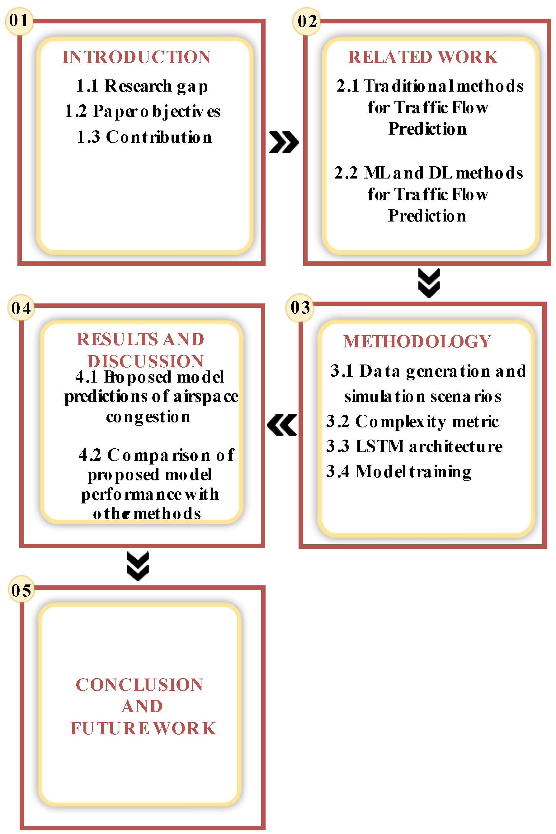
Figure 1. Structure of this study.
Drones 07 00078 g001
Figure 2. Simulation-scenario environment, with UAV missions map.
Drones 07 00078 g002
Figure 3. Scenario 3: 200 UAVs with extreme weather effects.
Drones 07 00078 g003
Figure 4. The dynamic system and its eigenvalues: for dynamic-system matrix A U ; the eigenvalue loci for two typical situations, namely, convergent (a) and divergent (b). One should note that the real component of the eigenvalues is negative only in the case of convergent trajectories. Meanwhile, the ‘neighborhood’ of a reference aircraft (for the computation of the complexity metric) is indicated by (c). (Adapted from the work of García et al. [29]).
Drones 07 00078 g004
Figure 5. LSTM for time series prediction—general architecture [82].
Drones 07 00078 g005
Figure 6. Overview of the proposition for the UTM traffic flow prediction model.
Drones 07 00078 g006
Figure 7. First scenario: Actual and predicted complexity in the airspace.
Drones 07 00078 g007
Figure 8. The difference between predicted and true congestion—Scenario 1.
Drones 07 00078 g008
Figure 9. Percentage residual complexity—Scenario 1.
Drones 07 00078 g009
Figure 10. Scenario 2: Actual and predicted complexity in the airspace.
Drones 07 00078 g010
Figure 11. The difference between predicted and true congestion—Scenario 2.
Drones 07 00078 g011
Figure 12. Percentage residual complexity—Scenario 2.
Drones 07 00078 g012
Figure 13. Scenario 3: Actual and predicted complexity in the airspace.
Drones 07 00078 g013
Figure 14. The difference between predicted and true congestion—Scenario 3.
Drones 07 00078 g014
Figure 15. Percentage residual complexity—Scenario 3.
Drones 07 00078 g015
Figure 16. Comparison of different prediction approaches.
Drones 07 00078 g016
Figure 17. Prediction vs. time for (a) shallow NN, (b) regression, and (c) proposed model.
Drones 07 00078 g017
Figure 18. Computation timing for shallow NN, regression, and proposed model.
Drones 07 00078 g018
Figure 19. Prediction timings percent increase.
Drones 07 00078 g019
Table 1. Airspace classes in accordance with ICAO guidelines [6].
Airspace ClassType of FlightSeparation
Provided by ATC
Comm. to ATCSubject to ATC Clear
Controlled airspaceAIFR onlyAll aircraftCont. 2-wayYes
BIFRAll aircraftCont. 2-wayYes
VFRAll aircraftCont. 2-wayYes
CIFRIFR from IFR
IFR from VFR
Cont. 2-wayYes
VFRVFR from IFRCont. 2-wayYes
DIFRIFR from IFRCont. 2-wayYes
VFRNoCont. 2-wayYes
EIFRIFR from IFRCont. 2-wayYes
VFRNoNot requiredNo
Uncontrolled airspaceFIFRIFR from IFR as far as practicalCont. 2-wayNo
VFRNoNot requiredNo
GIFRNoCont. 2-wayNo
VFRNoNot requiredNo
Table 2. The description and schedule for UAVs missions.
MissionCOVID-19 SamplesPackage DeliveryEmergency
Operation
Railway
Inspection
UAV fleetUAV1, UAV2 and UAV3UAV4 and UAV5UAV 6UAV7 and UAV8
Priority2314
RouteLutonUAV4UAV6 available atUAV7
CranfieldCardington Milton Keynes Bedford rail station
Milton KeynesGraveley Prison Fire Stationto Ridgmont
DunstableOld Warren
Sandy UAV8
Milton Keynes (MK) central rail station to Bletchley
UAV5
Cranfield
Dunstable
Halton
Milton Keynes
Scenario planningAll scenariosAll scenariosAll scenariosScenario 2 and 3
Table 3. Technical parameters of UAVs used during the simulation scenarios.
Parameters of UAVsValueUnit
UAV typeRotary wing--
Payload capacity25kg
Flight time30minutes
Cruise speed90km/h
Wind resistance10m/s
Table 4. List of the proposed model’s parameters.
ParameterDescription
ID A unique code is assigned to a single aircraft UAV to identify flight mission
P The UAV mission priority
t The timestep when the UAV is passing the waypoint
V UAV Velocity
HA Heading Angle
UAV StatesState = [Timestamp, Longitude, Latitude, Velocity, Heading Angle]
Complexity Metric
c A U
The complexity metric is a linear dynamic system model that identifies a complexity parameter in the vicinity of a UAV for a specified period of time.
Table 5. List of the proposed model’s hyperparameters values.
ParameterValue
Batch size128
(1-D) kernel width d3
(1-D) filter f512
Hidden layers (LSTM)128
ActivationReLU
OptimizerAdam optimizer [86]
Learning rate0.001
Epochs500
Loss functionRMSE
Disclaimer/Publisher’s Note: The statements, opinions and data contained in all publications are solely those of the individual author(s) and contributor(s) and not of MDPI and/or the editor(s). MDPI and/or the editor(s) disclaim responsibility for any injury to people or property resulting from any ideas, methods, instructions or products referred to in the content.