


UAV Path Planning Optimization Strategy: Considerations of Urban Morphology, Microclimate, and Energy Efficiency Using Q-Learning Algorithm


Abstract
:1. Introduction
- To promote a deep discussion regarding the challenges related to the UAVs’ flight autonomy during missions;
- To promote intelligent solutions based on machine learning by reinforcement to optimize the trajectory of UAVs under windy and urban scenarios;
- To promote numerous tests with the aim of investigating which reinforcement learning parameters are appropriate for the UAV route optimization problem considering physical obstacles and weather variation;
- To promote several tests exploring different positions of urban obstacles;
- To promote several tests that explore the insertion of high-incidence wind speed points in the scenario;
- To promote comparisons with other methodologies described in the literature based on reinforcement learning;
- To promote—through the simulation of numerical results—the efficiency of the strategy proposed herein; thus, attesting to its potential as a solution.
2. Related Work
3. Preliminary
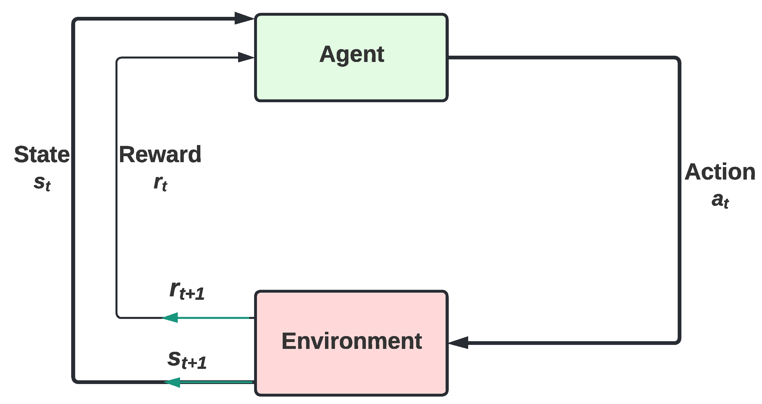
3.1. Reinforcement Learning (RL)
3.2. SARSA
3.3. Q-Learning
3.4. Exploration and Exploitation
3.5. ϵ-Greedy
3.6. ϵ-Greedy Decay
3.7. Assumptions
- The UAV knows its position at all times;
- The final destination and the goal of each heuristic subprocess are known to the UAV;
- The route calculation takes place independently between the UAVS;
- The height of the buildings is randomly arranged;
- Obstacles are all buildings and structures whose length is more than 120 m;
- The speed of the UAVS is constant;
- The velocity vector of the UAVs will always be opposite to the wind speed.
4. Proposed Solution
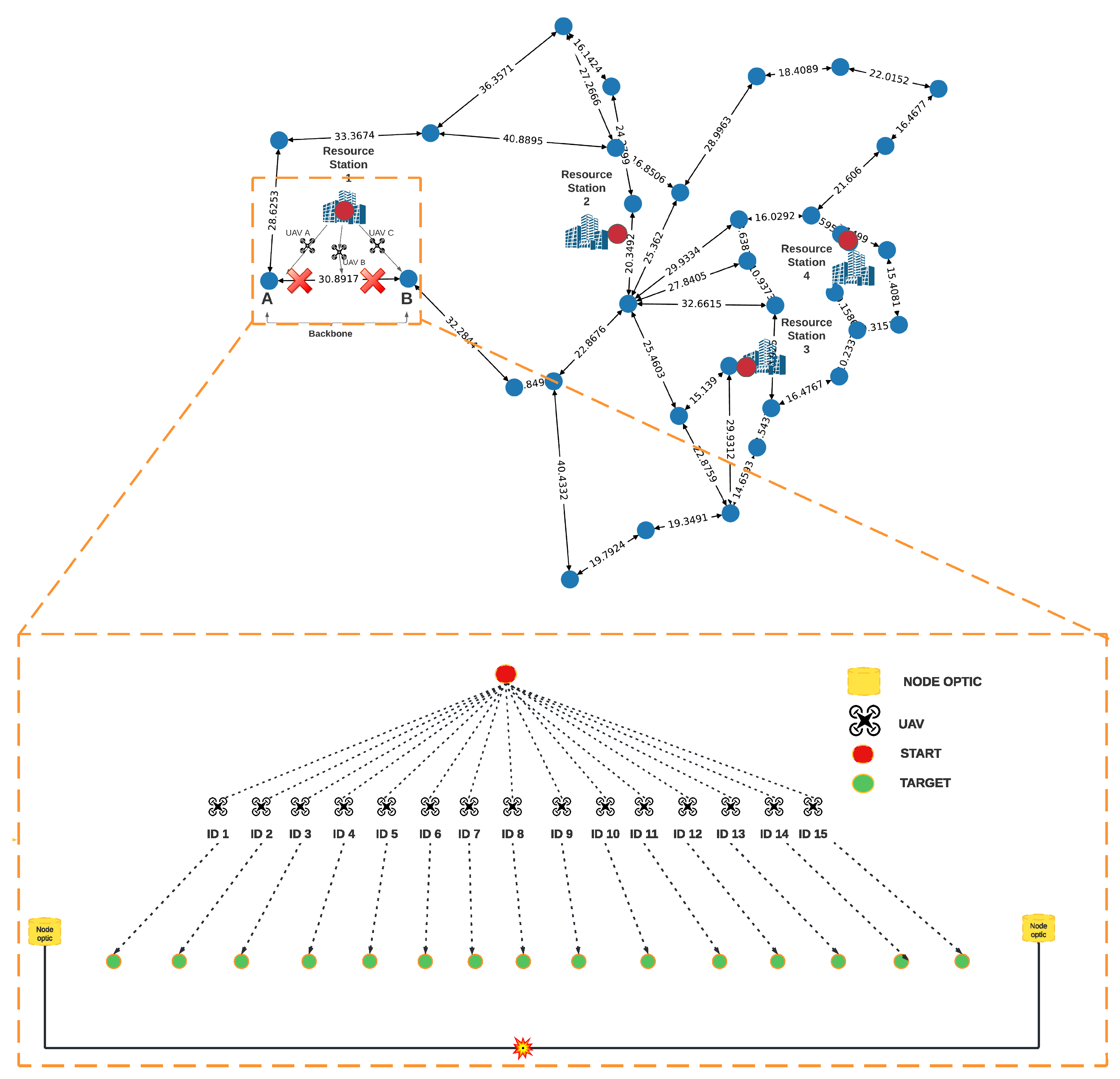
4.1. Positioning Strategy for Resource Stations
| Algorithm 1 k-means algorithm for position of resource bases and energy loading |
| Input: Network Graph |
| Output: Set of datasets clusters DC |
|
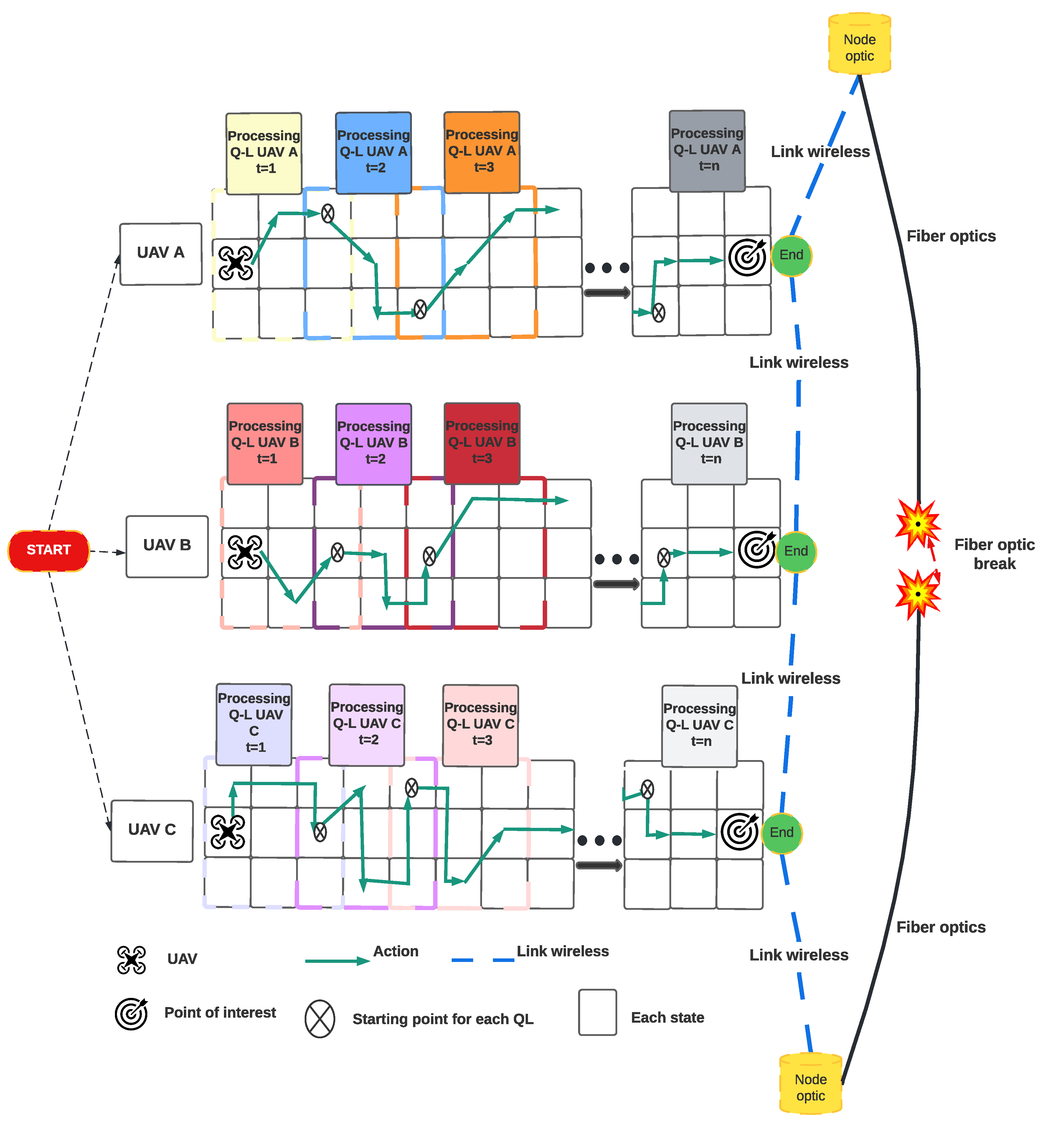
4.2. UAV Travel Strategy Based on Q-Learning
| Algorithm 2 Q-learning for UAV route optimization |
| Input: Q-table, , , R, , , |
| Output: Optimal strategy , Optimal router UAV |
|
4.2.1. Agents
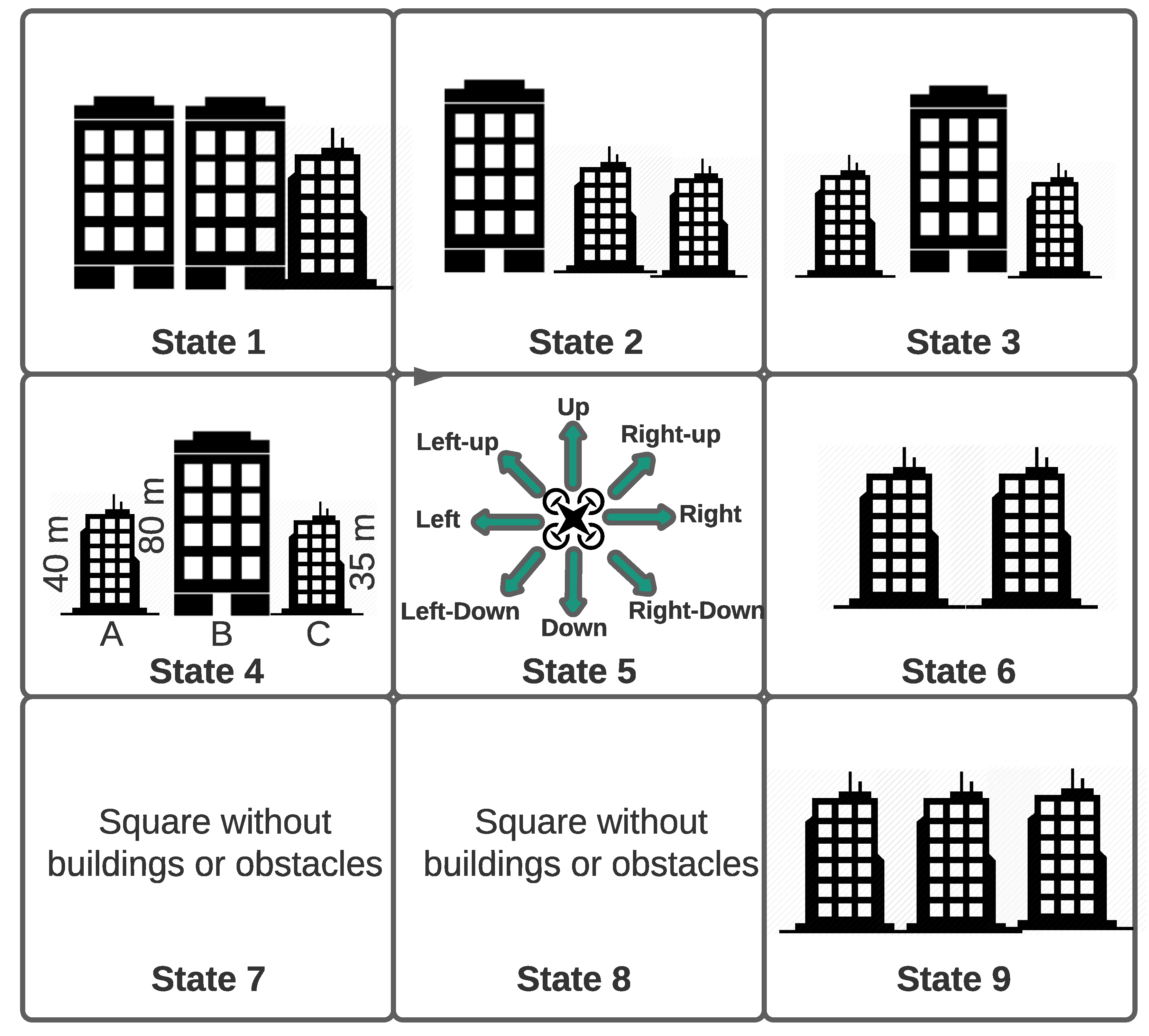
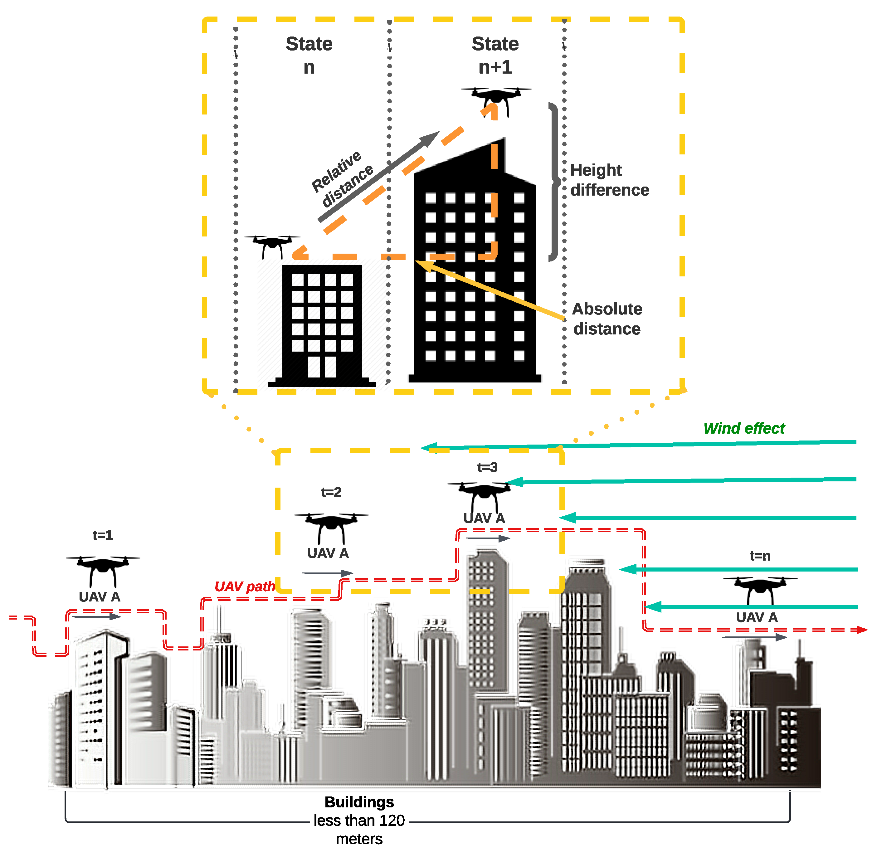
4.2.2. States
4.2.3. Actions
4.2.4. Reward
4.2.5. Q Strategy
4.2.6. Algorithm Initialization
4.2.7. Stopping Criteria
4.3. Evaluation Metrics
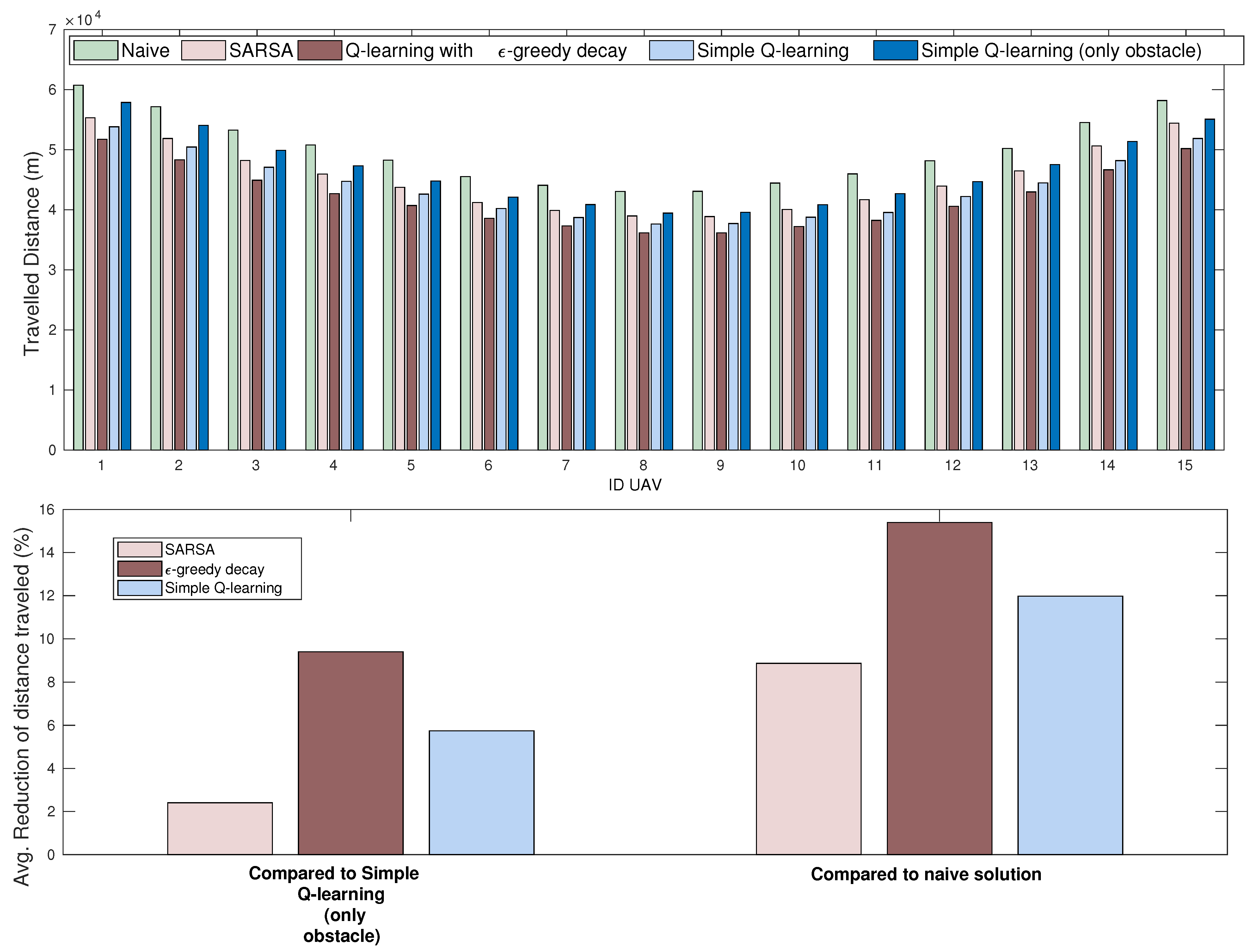
4.3.1. Distance Traveled
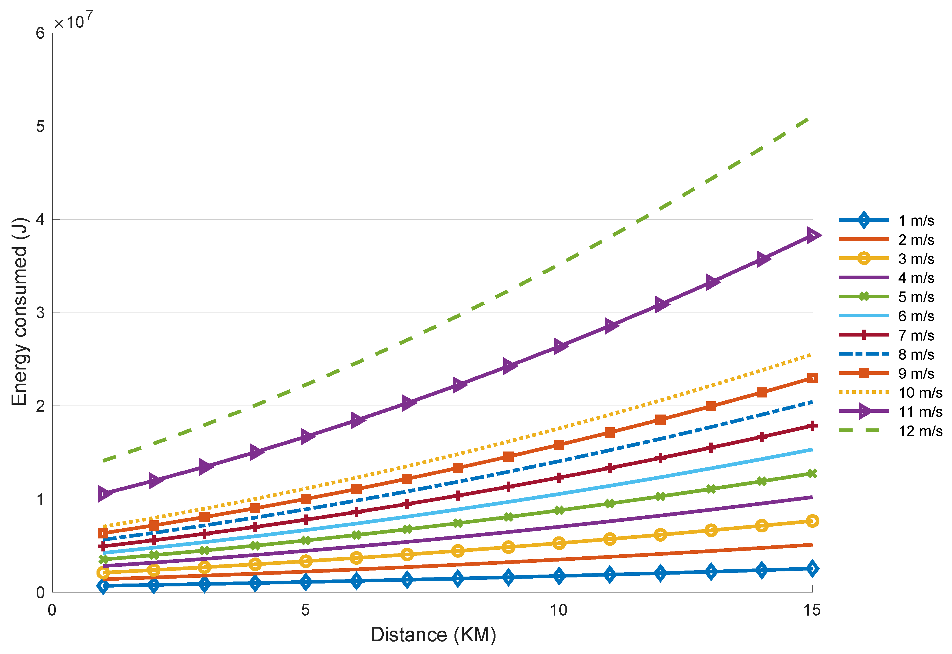
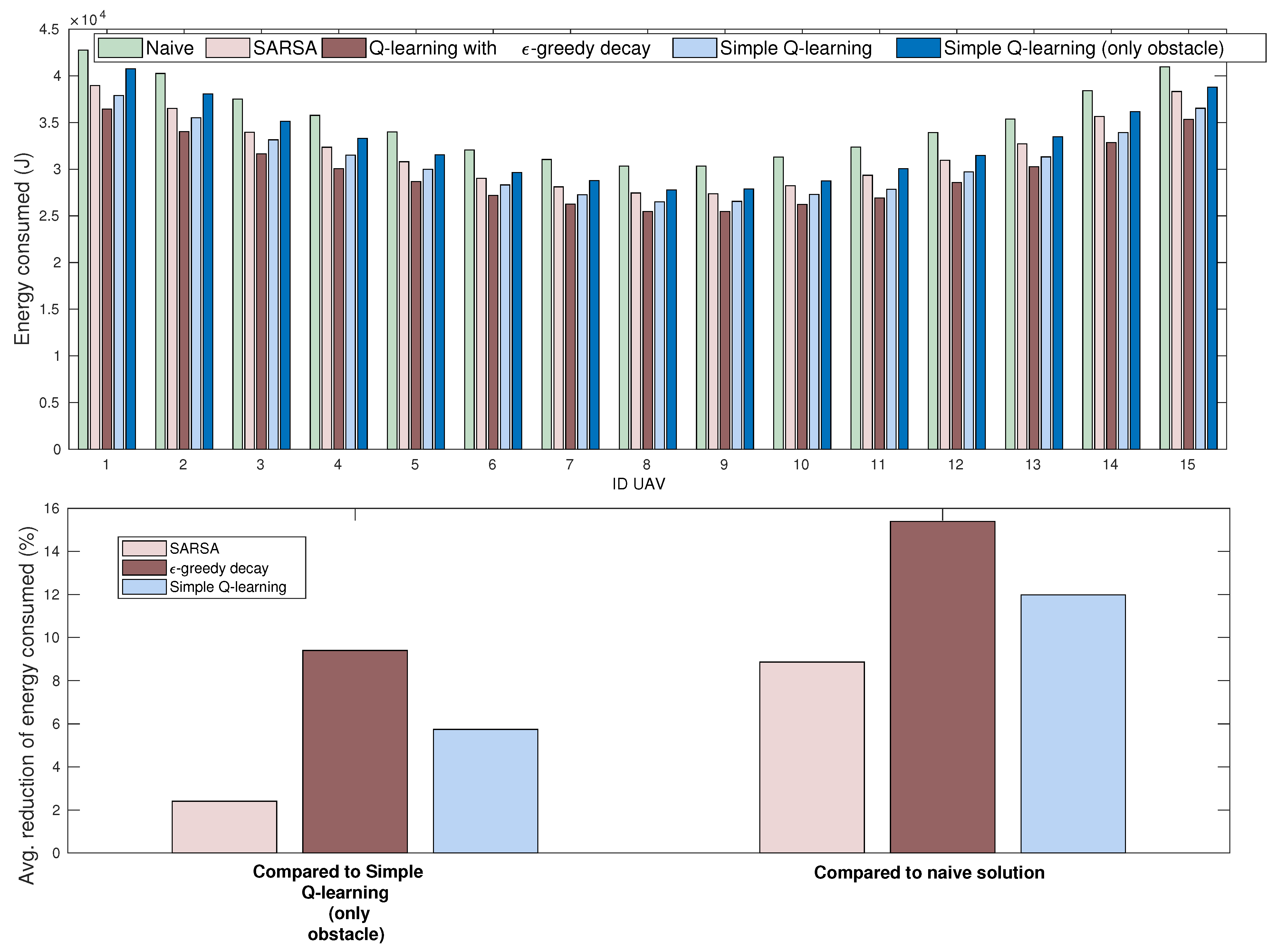
4.3.2. Energy Consumer
4.3.3. Success Rate
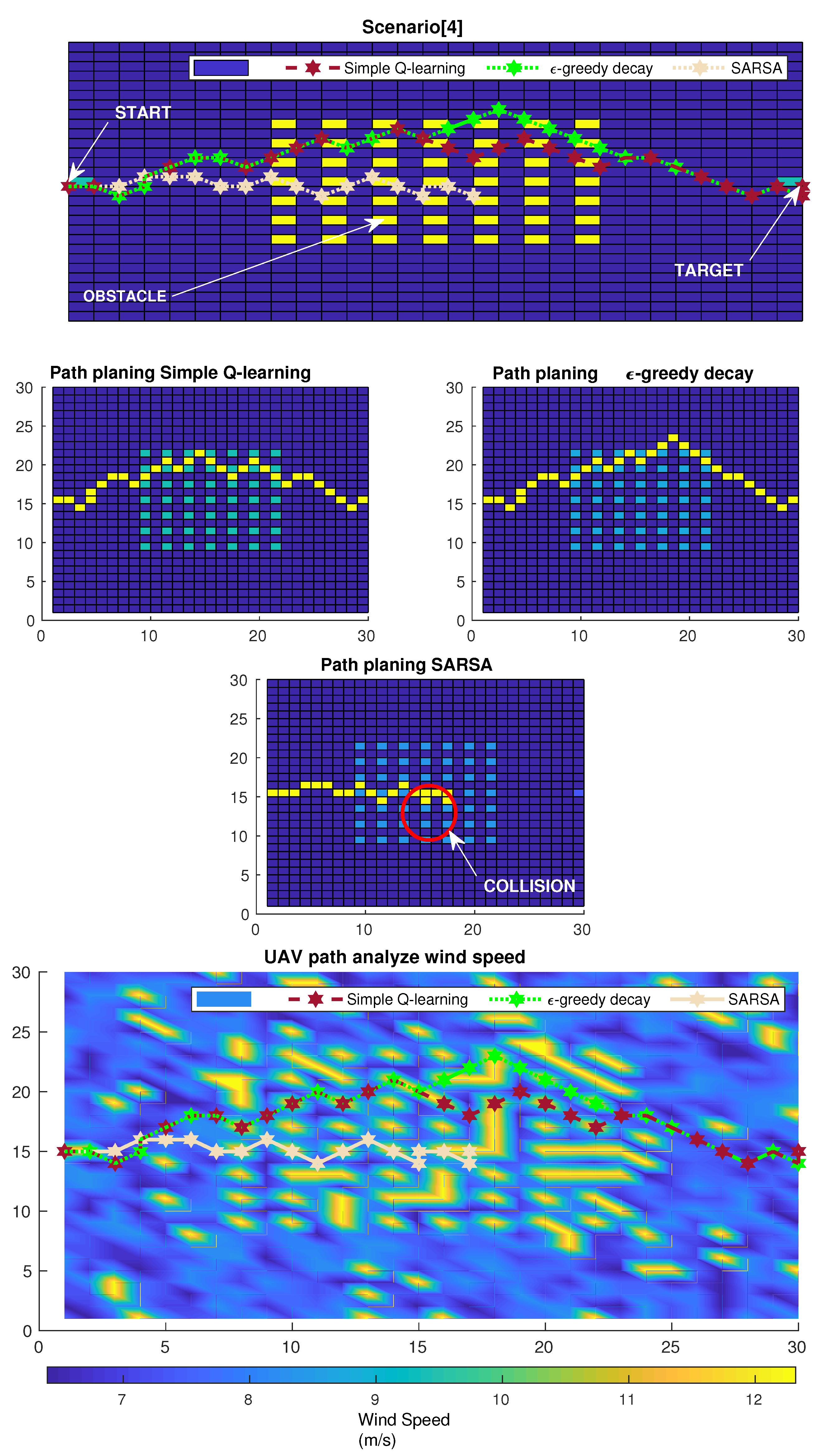
4.3.4. Wind Speed
5. Experiments and Tests
5.1. Experiment 1
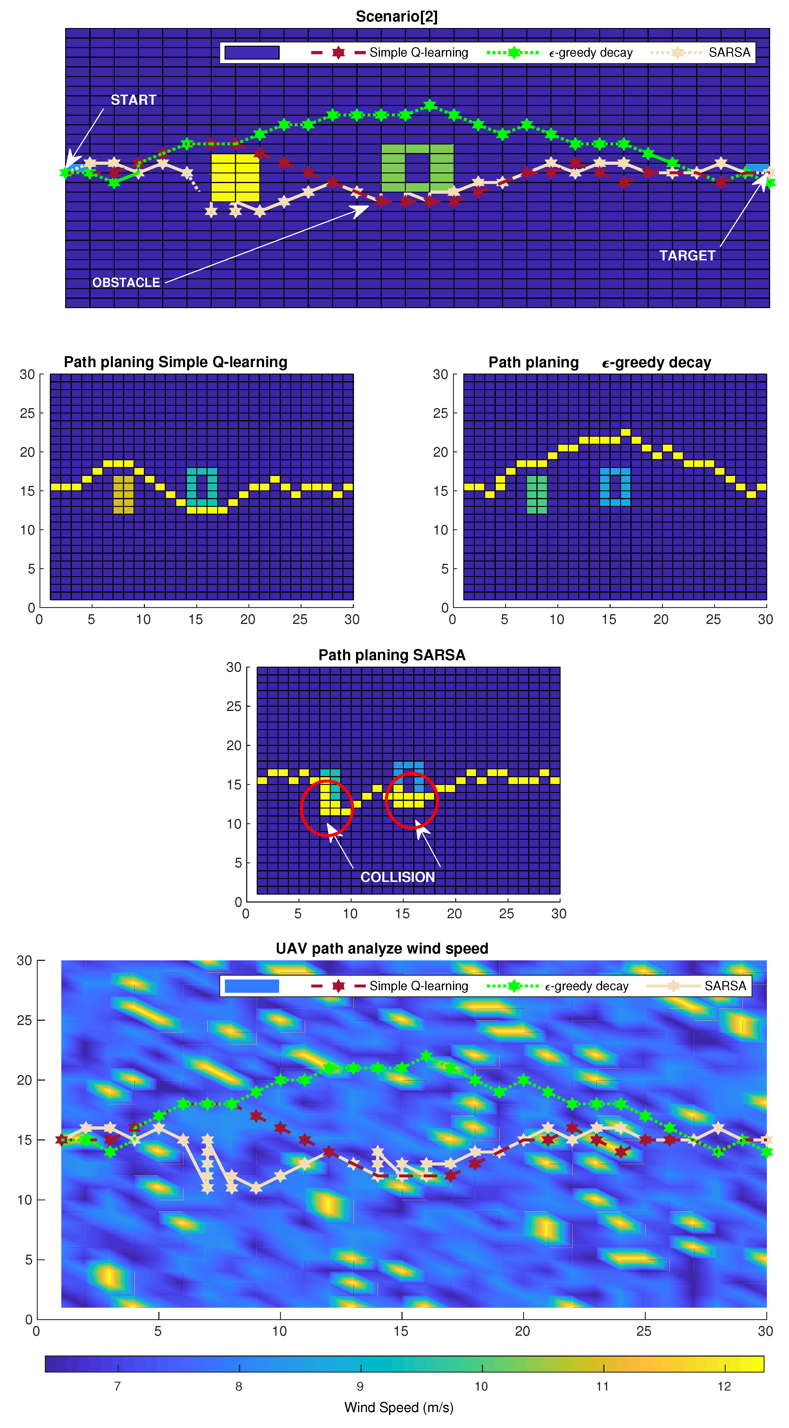
5.2. Experiment 2
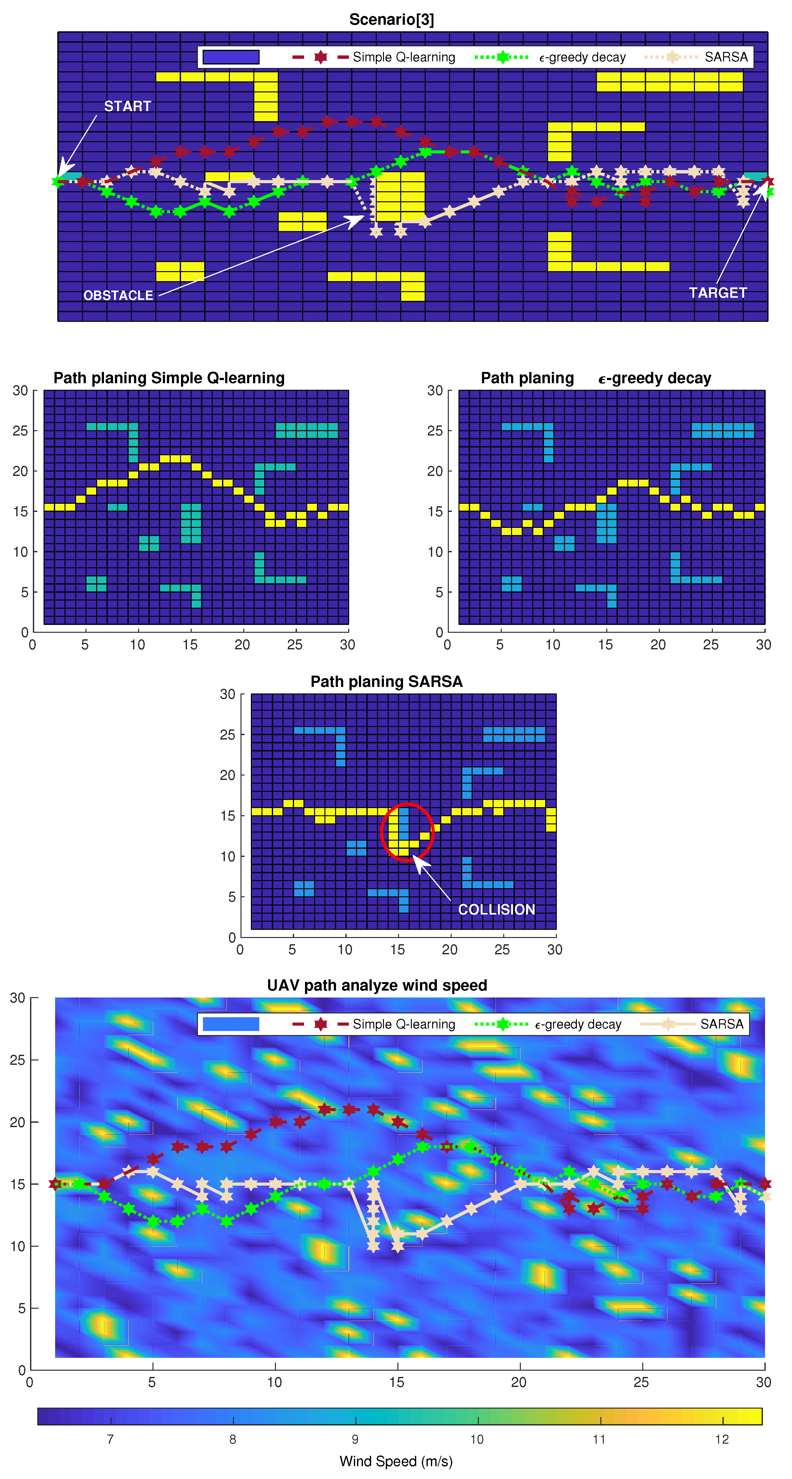
5.3. Experiment 3
5.4. Experiment 4
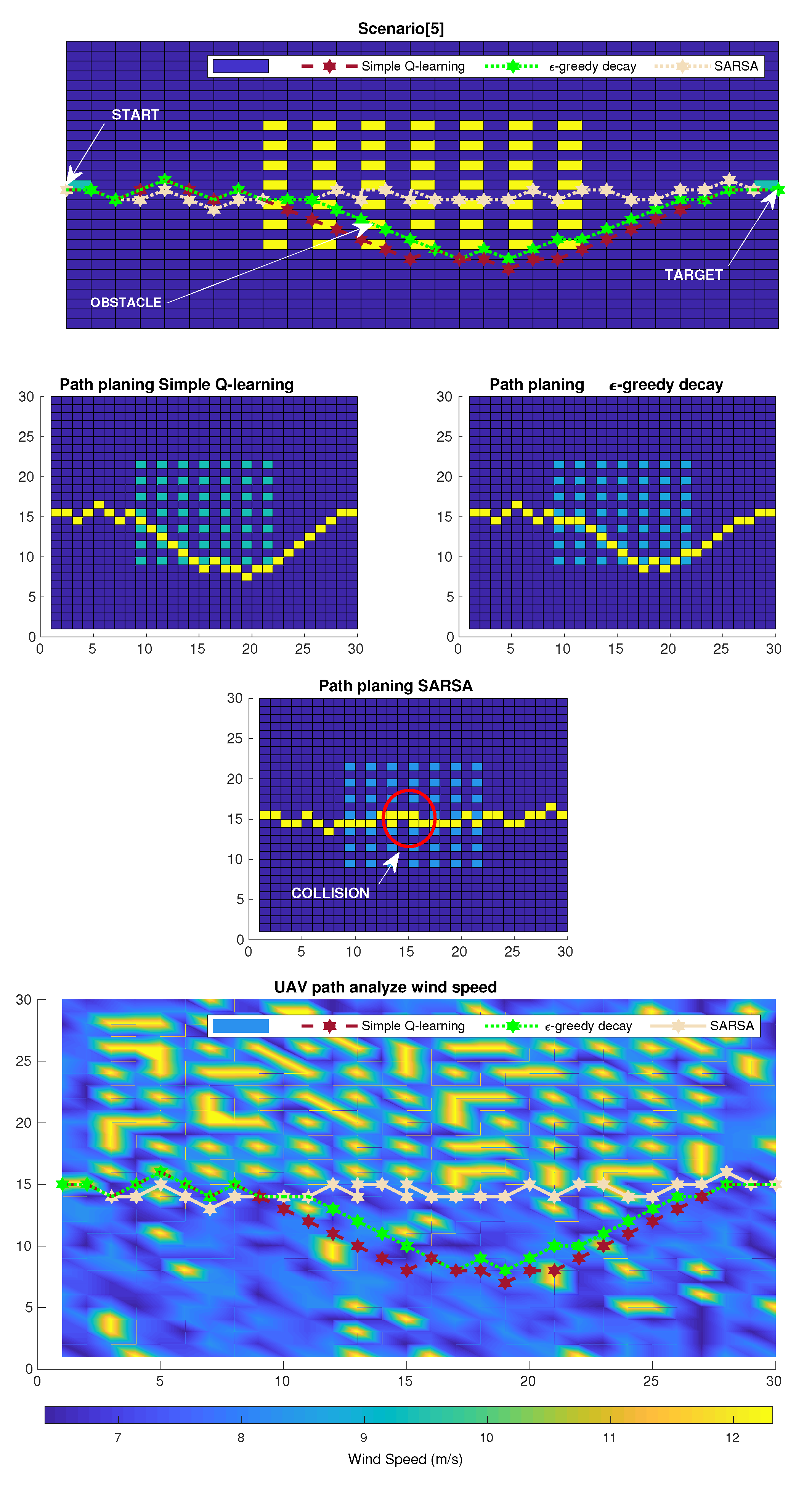
5.5. Experiment 5
6. Simulation Results
6.1. Simulation Scenario
6.2. Numerical Results
6.3. Results and Discussion
7. Conclusions
Author Contributions
Funding
Institutional Review Board Statement
Informed Consent Statement
Data Availability Statement
Acknowledgments
Conflicts of Interest
Abbreviations
| UAV | Unmanned aerial vehicles |
| CIT | Information and communication technology |
| BANs | Body area networks |
| LoS | Line of sight |
| NTSB | The National Transportation Safety Board |
| SARSA | (State − action − reward − state − action) |
| MDP | Markov Decision Process |
| VTOL | Vertical Take-Off and Landing |
| FSO | Free-space optics |
| Q-L | Q-learning |
| Obstacle weights | |
| Wind speed weights | |
| Distance weights | |
| Obstacle reward | |
| Wind speed reward | |
| Distance of target reward | |
| Obstacle reward | |
| Maximum wind speed | |
| Absolute distance | |
| K | Mumber of UAVS |
| Propulsion speed | |
| D | Distance travaled |
| m | Payload |
| Relative distance | |
| Height of the building | |
| Roughness factor | |
| Altitude to calculate the speed | |
| Initial altitude the speed | |
| UAV speed | |
| Wind speed | |
| Discount rate | |
| Learning rate |
References
- Dagooc, E.M. IBM urged LGUs to embrace the’Smarter city’initiative. Philipp. Star. Retrieved March 2010, 3, 2011. [Google Scholar]
- Mosannenzadeh, F.; Vettorato, D. Defining smart city. A conceptual framework based on keyword analysis. TeMA-J. Land Use Mobil. Environ. 2014, 16, 684–694. [Google Scholar] [CrossRef]
- Sánchez-Corcuera, R.; Nuñez-Marcos, A.; Sesma-Solance, J.; Bilbao-Jayo, A.; Mulero, R.; Zulaika, U.; Azkune, G.; Almeida, A. Smart cities survey: Technologies, application domains and challenges for the cities of the future. Int. J. Distrib. Sens. Netw. 2019, 15, 1550147719853984. [Google Scholar] [CrossRef]
- Visvizi, A.; Lytras, M.D.; Damiani, E.; Mathkour, H. Policy making for smart cities: Innovation and social inclusive economic growth for sustainability. J. Sci. Technol. Policy Manag. 2018, 9, 126–133. [Google Scholar] [CrossRef]
- Silva, B.N.; Khan, M.; Han, K. Towards sustainable smart cities: A review of trends, architectures, components, and open challenges in smart cities. Sustain. Cities Soc. 2018, 38, 697–713. [Google Scholar] [CrossRef]
- Medina-Borja, A. Editorial column—Smart things as service providers: A call for convergence of disciplines to build a research agenda for the service systems of the future. Serv. Sci. 2015, 7, 2–5. [Google Scholar] [CrossRef]
- Gupta, L.; Jain, R.; Vaszkun, G. Survey of important issues in UAV communication networks. IEEE Commun. Surv. Tutorials 2015, 18, 1123–1152. [Google Scholar] [CrossRef]
- Mehta, P.; Gupta, R.; Tanwar, S. Blockchain envisioned UAV networks: Challenges, solutions, and comparisons. Comput. Commun. 2020, 151, 518–538. [Google Scholar] [CrossRef]
- Maddikunta, P.K.R.; Hakak, S.; Alazab, M.; Bhattacharya, S.; Gadekallu, T.R.; Khan, W.Z.; Pham, Q.V. Unmanned aerial vehicles in smart agriculture: Applications, requirements, and challenges. IEEE Sensors J. 2021, 21, 17608–17619. [Google Scholar] [CrossRef]
- De Alwis, C.; Kalla, A.; Pham, Q.V.; Kumar, P.; Dev, K.; Hwang, W.J.; Liyanage, M. Survey on 6G frontiers: Trends, applications, requirements, technologies and future research. IEEE Open J. Commun. Soc. 2021, 2, 836–886. [Google Scholar] [CrossRef]
- Tisdale, J.; Kim, Z.; Hedrick, J.K. Autonomous UAV path planning and estimation. IEEE Robot. Autom. Mag. 2009, 16, 35–42. [Google Scholar] [CrossRef]
- Grasso, C.; Schembra, G. Design of a UAV-based videosurveillance system with tactile internet constraints in a 5G ecosystem. In Proceedings of the 2018 4th IEEE Conference on Network Softwarization and Workshops (NetSoft), Montreal, QC, Canada, 25–29 June 2018; pp. 449–455. [Google Scholar]
- Ullah, S.; Kim, K.I.; Kim, K.H.; Imran, M.; Khan, P.; Tovar, E.; Ali, F. UAV-enabled healthcare architecture: Issues and challenges. Future Gener. Comput. Syst. 2019, 97, 425–432. [Google Scholar] [CrossRef]
- Tang, C.; Zhu, C.; Wei, X.; Rodrigues, J.J.; Guizani, M.; Jia, W. UAV placement optimization for Internet of Medical Things. In Proceedings of the 2020 International Wireless Communications and Mobile Computing (IWCMC), Limassol, Cyprus, 15–19 June 2020; pp. 752–757. [Google Scholar]
- Mozaffari, M.; Kasgari, A.T.Z.; Saad, W.; Bennis, M.; Debbah, M. Beyond 5G with UAVs: Foundations of a 3D wireless cellular network. IEEE Trans. Wirel. Commun. 2018, 18, 357–372. [Google Scholar] [CrossRef]
- Li, B.; Fei, Z.; Zhang, Y. UAV communications for 5G and beyond: Recent advances and future trends. IEEE Internet Things J. 2018, 6, 2241–2263. [Google Scholar] [CrossRef]
- Pham, Q.V.; Zeng, M.; Ruby, R.; Huynh-The, T.; Hwang, W.J. UAV Communications for Sustainable Federated Learning. IEEE Trans. Veh. Technol. 2021, 70, 3944–3948. [Google Scholar] [CrossRef]
- Zeng, Y.; Zhang, R.; Lim, T.J. Wireless communications with unmanned aerial vehicles: Opportunities and challenges. IEEE Commun. Mag. 2016, 54, 36–42. [Google Scholar] [CrossRef]
- Şahin, H.; Kose, O.; Oktay, T. Simultaneous autonomous system and powerplant design for morphing quadrotors. Aircr. Eng. Aerosp. Technol. 2022, 94, 1228–1241. [Google Scholar] [CrossRef]
- Zeng, Y.; Zhang, R. Energy-efficient UAV communication with trajectory optimization. IEEE Trans. Wirel. Commun. 2017, 16, 3747–3760. [Google Scholar] [CrossRef]
- Wu, F.; Yang, D.; Xiao, L.; Cuthbert, L. Energy consumption and completion time tradeoff in rotary-wing UAV enabled WPCN. IEEE Access 2019, 7, 79617–79635. [Google Scholar] [CrossRef]
- PAHL, J. Flight recorders in accident and incident investigation. In Proceedings of the 1st Annual Meeting, Washington, DC, USA, 29 June–2 July 1964; p. 351. [Google Scholar]
- Lester, A. Global air transport accident statistics. In Proceedings of the Aviation Safety Meeting, Toronto, ON, Canada, 31 October–1 November 1966; p. 805. [Google Scholar]
- Li, W.; Wang, L.; Fei, A. Minimizing packet expiration loss with path planning in UAV-assisted data sensing. IEEE Wirel. Commun. Lett. 2019, 8, 1520–1523. [Google Scholar] [CrossRef]
- Hermand, E.; Nguyen, T.W.; Hosseinzadeh, M.; Garone, E. Constrained control of UAVs in geofencing applications. In Proceedings of the 2018 26th Mediterranean Conference on Control and Automation (MED), Zadar, Croatia, 19–22 June 2018; pp. 217–222. [Google Scholar]
- Ariante, G.; Ponte, S.; Papa, U.; Greco, A.; Del Core, G. Ground Control System for UAS Safe Landing Area Determination (SLAD) in Urban Air Mobility Operations. Sensors 2022, 22, 3226. [Google Scholar] [CrossRef] [PubMed]
- Jayaweera, H.M.; Hanoun, S. Path Planning of Unmanned Aerial Vehicles (UAVs) in Windy Environments. Drones 2022, 6, 101. [Google Scholar] [CrossRef]
- Cao, P.; Liu, Y.; Yang, C.; Xie, S.; Xie, K. MEC-Driven UAV-Enabled Routine Inspection Scheme in Wind Farm Under Wind Influence. IEEE Access 2019, 7, 179252–179265. [Google Scholar] [CrossRef]
- Tseng, C.M.; Chau, C.K.; Elbassioni, K.M.; Khonji, M. Flight Tour Planning with Recharging Optimization for Battery-Operated Autonomous Drones. CoRR 2017. Available online: https://www.researchgate.net/profile/Majid-Khonji/publication/315695709_Flight_Tour_Planning_with_Recharging_Optimization_for_Battery-operated_Autonomous_Drones/links/58fff4cfaca2725bd71e7a69/Flight-Tour-Planning-with-Recharging-Optimization-for-Battery-operated-Autonomous-Drones.pdf (accessed on 24 October 2022).
- Thibbotuwawa, A. Unmanned Aerial Vehicle Fleet Mission Planning Subject to Changing Weather Conditions. Ph. D. Thesis, Og Naturvidenskabelige Fakultet, Aalborg Universitet, Aalborg, Denmark, 2019. [Google Scholar]
- Thibbotuwawa, A.; Bocewicz, G.; Zbigniew, B.; Nielsen, P. A solution approach for UAV fleet mission planning in changing weather conditions. Appl. Sci. 2019, 9, 3972. [Google Scholar] [CrossRef]
- Thibbotuwawa, A.; Bocewicz, G.; Radzki, G.; Nielsen, P.; Banaszak, Z. UAV Mission planning resistant to weather uncertainty. Sensors 2020, 20, 515. [Google Scholar] [CrossRef]
- Dorling, K.; Heinrichs, J.; Messier, G.G.; Magierowski, S. Vehicle routing problems for drone delivery. IEEE Trans. Syst. Man, Cybern. Syst. 2016, 47, 70–85. [Google Scholar] [CrossRef]
- Klaine, P.V.; Nadas, J.P.; Souza, R.D.; Imran, M.A. Distributed drone base station positioning for emergency cellular networks using reinforcement learning. Cogn. Comput. 2018, 10, 790–804. [Google Scholar] [CrossRef]
- Zhao, C.; Liu, J.; Sheng, M.; Teng, W.; Zheng, Y.; Li, J. Multi-UAV Trajectory Planning for Energy-efficient Content Coverage: A Decentralized Learning-Based Approach. IEEE J. Sel. Areas Commun. 2021, 39, 3193–3207. [Google Scholar] [CrossRef]
- Hu, J.; Zhang, H.; Song, L. Reinforcement learning for decentralized trajectory design in cellular UAV networks with sense-and-send protocol. IEEE Internet Things J. 2018, 6, 6177–6189. [Google Scholar] [CrossRef]
- Saxena, V.; Jaldén, J.; Klessig, H. Optimal UAV base station trajectories using flow-level models for reinforcement learning. IEEE Trans. Cogn. Commun. Netw. 2019, 5, 1101–1112. [Google Scholar] [CrossRef]
- Liu, C.H.; Chen, Z.; Tang, J.; Xu, J.; Piao, C. Energy-efficient UAV control for effective and fair communication coverage: A deep reinforcement learning approach. IEEE J. Sel. Areas Commun. 2018, 36, 2059–2070. [Google Scholar] [CrossRef]
- ur Rahman, S.; Kim, G.H.; Cho, Y.Z.; Khan, A. Positioning of UAVs for throughput maximization in software-defined disaster area UAV communication networks. J. Commun. Netw. 2018, 20, 452–463. [Google Scholar] [CrossRef]
- Zhang, Z.; Wu, J.; He, C. Search Method of disaster inspection coordinated by Multi-UAV. In Proceedings of the 2019 Chinese Control Conference (CCC), Guangzhou, China, 27–30 July 2019; pp. 2144–2148. [Google Scholar]
- Zhang, S.; Cheng, W. Statistical QoS Provisioning for UAV-Enabled Emergency Communication Networks. In Proceedings of the 2019 IEEE Globecom Workshops (GC Wkshps), Waikoloa, HI, USA, 9–13 December 2019; pp. 1–6. [Google Scholar]
- Sánchez-García, J.; Reina, D.; Toral, S. A distributed PSO-based exploration algorithm for a UAV network assisting a disaster scenario. Future Gener. Comput. Syst. 2019, 90, 129–148. [Google Scholar] [CrossRef]
- Sánchez-García, J.; García-Campos, J.M.; Toral, S.; Reina, D.; Barrero, F. An intelligent strategy for tactical movements of UAVs in disaster scenarios. Int. J. Distrib. Sens. Netw. 2016, 12, 8132812. [Google Scholar] [CrossRef]
- Ghamry, K.A.; Kamel, M.A.; Zhang, Y. Multiple UAVs in forest fire fighting mission using particle swarm optimization. In Proceedings of the 2017 International Conference on Unmanned Aircraft Systems (ICUAS), Miami, FL, USA, 13–16 June 2017; pp. 1404–1409. [Google Scholar]
- Sanci, E.; Daskin, M.S. Integrating location and network restoration decisions in relief networks under uncertainty. Eur. J. Oper. Res. 2019, 279, 335–350. [Google Scholar] [CrossRef]
- Mekikis, P.V.; Antonopoulos, A.; Kartsakli, E.; Alonso, L.; Verikoukis, C. Communication recovery with emergency aerial networks. IEEE Trans. Consum. Electron. 2017, 63, 291–299. [Google Scholar] [CrossRef]
- Agrawal, A.; Bhatia, V.; Prakash, S. Network and risk modeling for disaster survivability analysis of backbone optical communication networks. J. Light. Technol. 2019, 37, 2352–2362. [Google Scholar] [CrossRef]
- Tran, P.N.; Saito, H. Enhancing physical network robustness against earthquake disasters with additional links. J. Light. Technol. 2016, 34, 5226–5238. [Google Scholar] [CrossRef]
- Ma, C.; Zhang, J.; Zhao, Y.; Habib, M.F.; Savas, S.S.; Mukherjee, B. Traveling repairman problem for optical network recovery to restore virtual networks after a disaster. IEEE/OSA J. Opt. Commun. Netw. 2015, 7, B81–B92. [Google Scholar] [CrossRef]
- Msongaleli, D.L.; Dikbiyik, F.; Zukerman, M.; Mukherjee, B. Disaster-aware submarine fiber-optic cable deployment for mesh networks. J. Light. Technol. 2016, 34, 4293–4303. [Google Scholar] [CrossRef]
- Dikbiyik, F.; Tornatore, M.; Mukherjee, B. Minimizing the risk from disaster failures in optical backbone networks. J. Light. Technol. 2014, 32, 3175–3183. [Google Scholar] [CrossRef]
- Abdallah, A.; Ali, M.Z.; Mišić, J.; Mišić, V.B. Efficient Security Scheme for Disaster Surveillance UAV Communication Networks. Information 2019, 10, 43. [Google Scholar] [CrossRef]
- Sutton, R.S.; Barto, A.G. Reinforcement learning. J. Cogn. Neurosci. 1999, 11, 126–134. [Google Scholar]
- Rummery, G.A.; Niranjan, M. On-Line Q-Learning Using Connectionist Systems; University of Cambridge, Department of Engineering: Cambridge, UK, 1994; Volume 37. [Google Scholar]
- Watkins, C.J.C.H. Learning from Delayed Rewards; University of Cambridge: Cambridge, UK, 1989. [Google Scholar]
- Watkins, C.J.; Dayan, P. Q-learning. Mach. Learn. 1992, 8, 279–292. [Google Scholar] [CrossRef]
- Tokic, M.; Palm, G. Value-difference based exploration: Adaptive control between epsilon-greedy and softmax. In Annual Conference on Artificial Intelligence; Springer: Berlin/Heidelberg, Germany, 2011; pp. 335–346. [Google Scholar]
- Tsitsiklis, J.N. Asynchronous stochastic approximation and Q-learning. Mach. Learn. 1994, 16, 185–202. [Google Scholar] [CrossRef]
- Thrun, S.B. Efficient Exploration in Reinforcement Learning. 1992. Available online: https://www.ri.cmu.edu/pub_files/pub1/thrun_sebastian_1992_1/thrun_sebastian_1992_1.pdf (accessed on 24 October 2022).
- Auer, P. Using confidence bounds for exploitation-exploration trade-offs. J. Mach. Learn. Res. 2002, 3, 397–422. [Google Scholar]
- Kumar, V.; Webster, M. Importance Sampling based Exploration in Q Learning. arXiv 2021, arXiv:2107.00602. [Google Scholar]
- Dabney, W.; Ostrovski, G.; Barreto, A. Temporally-extended ε-greedy exploration. arXiv 2020, arXiv:2006.01782. [Google Scholar]
- Ludwig, N. 14 CFR Part 107 (UAS)–Drone Operators Are Not Pilots. Available online: https://www.suasnews.com/2017/12/14-cfr-part-107-uas-drone-operators-not-pilots/ (accessed on 24 October 2022).
- Eole, S. Windenergie-Daten der Schweiz. 2010. Available online: http://www.wind-data.ch/windkarte/ (accessed on 24 October 2022).
- Delgado, A.; Gertig, C.; Blesa, E.; Loza, A.; Hidalgo, C.; Ron, R. Evaluation of the variability of wind speed at different heights and its impact on the receiver efficiency of central receiver systems. In AIP Conference Proceedings; AIP Publishing LLC: Cape Town, South Africa, 2015; Volume 1734, p. 030011. [Google Scholar]
- Fang, P.; Jiang, W.; Tang, J.; Lei, X.; Tan, J. Variations in friction velocity with wind speed and height for moderate-to-strong onshore winds based on Measurements from a coastal tower. J. Appl. Meteorol. Climatol. 2020, 59, 637–650. [Google Scholar] [CrossRef]
- Mohandes, M.; Rehman, S.; Nuha, H.; Islam, M.; Schulze, F. Wind speed predictability accuracy with height using LiDAR based measurements and artificial neural networks. Appl. Artif. Intell. 2021, 35, 605–622. [Google Scholar] [CrossRef]
- Cui, Z.; Wang, Y. UAV path planning based on multi-layer reinforcement learning technique. IEEE Access 2021, 9, 59486–59497. [Google Scholar] [CrossRef]
- Chung, H.M.; Maharjan, S.; Zhang, Y.; Eliassen, F.; Strunz, K. Placement and Routing Optimization for Automated Inspection With Unmanned Aerial Vehicles: A Study in Offshore Wind Farm. IEEE Trans. Ind. Inform. 2020, 17, 3032–3043. [Google Scholar] [CrossRef]
- Hou, Y.; Huang, W.; Zhou, H.; Gu, F.; Chang, Y.; He, Y. Analysis on Wind Resistance Index of Multi-rotor UAV. In Proceedings of the 2019 Chinese Control And Decision Conference (CCDC), Nanchang, China, 3–5 June 2019; pp. 3693–3696. [Google Scholar]
- Die Website Für Windenergie-Daten der Schweiz. Available online: http://www.wind-data.ch/tools/ (accessed on 24 October 2022).
- Cardoso, E.; Natalino, C.; Alfaia, R.; Souto, A.; Araújo, J.; Francês, C.R.; Chiaraviglio, L.; Monti, P. A heuristic approach for the design of UAV-based disaster relief in optical metro networks. In Proceedings of the 2020 22nd International Conference on Transparent Optical Networks (ICTON), Bari, Italy, 19–23 July 2020; pp. 1–5. [Google Scholar]
- Fawaz, W.; Abou-Rjeily, C.; Assi, C. UAV-aided cooperation for FSO communication systems. IEEE Commun. Mag. 2018, 56, 70–75. [Google Scholar] [CrossRef]
- Zhou, M.K.; Hu, Z.K.; Duan, X.C.; Sun, B.L.; Zhao, J.B.; Luo, J. Experimental progress in gravity measurement with an atom interferometer. Front. Phys. China 2009, 4, 170–173. [Google Scholar] [CrossRef]
- Jarchi, D.; Casson, A.J. Description of a database containing wrist PPG signals recorded during physical exercise with both accelerometer and gyroscope measures of motion. Data 2016, 2, 1. [Google Scholar] [CrossRef]
- Yu, L.; Yan, X.; Kuang, Z.; Chen, B.; Zhao, Y. Driverless bus path tracking based on fuzzy pure pursuit control with a front axle reference. Appl. Sci. 2019, 10, 230. [Google Scholar] [CrossRef]


| Roughness Length | Land Cover Types |
|---|---|
| 0.0002 m | Water surfaces: seas and Lakes |
| 0.0024 m | Open terrain with smooth surface, e.g., concrete, airport runways, mown grass, etc. |
| 0.03 m | Open agricultural land without fences and hedges; maybe some far apart buildings and very gentle hills |
| 0.055 m | Agricultural land with a few buildings and 8 m high hedges separated by more than 1 km |
| 0.1 m | Agricultural land with a few buildings and 8 m high hedges seperated by approx. 500 m |
| 0.2 m | Agricultural land with many trees, bushes, and plants, or 8 m high hedges separated by approx. 250 m |
| 0.4 m | Towns, villages, agricultural land with many or high hedges, forests and very rough and uneven terrain |
| 0.6 m | Large towns with high buildings |
| 1.6 m | Large cities with high buildings and skyscrapers |
| Experiment | Number of Obstacle | Arrangement of High Wind Speed Points in the Scenario |
|---|---|---|
| 1 | 1 | Randomly |
| 2 | 2 | Randomly |
| 3 | 9 | Randomly |
| 4 | 49 (in the center) | In the center |
| 5 | 49 (in the center) | in the upper half |
| Parameter | Value |
|---|---|
| Total Payload | 90 kg [32] |
| UAV speed | 15 m/s |
| Number of UAVs | 15 |
| Maximum distance between UAVs aerial links | 2 km |
| Number of Resource stations | 4 |
| Maximum wind speed | 13 m/s |
| Minimum wind speed | 6 m/s |
| Minimum height of obstacles | 30 m |
| Maximum height of obstacles | 121 m |
| Gravity acceleration (g) | 9.8 m/s [74,75,76] |
| Maximum exploration rate () | 1 |
| Minimum exploration rate ( ) | 0 |
| Roughness factor() | 1.6 m |
| Initial wind speed () | 5 m/s |
| Initial altitude the speed () | 8.5 m |
| Exploration decay rate | 0.01 |
Disclaimer/Publisher’s Note: The statements, opinions and data contained in all publications are solely those of the individual author(s) and contributor(s) and not of MDPI and/or the editor(s). MDPI and/or the editor(s) disclaim responsibility for any injury to people or property resulting from any ideas, methods, instructions or products referred to in the content. |
© 2023 by the authors. Licensee MDPI, Basel, Switzerland. This article is an open access article distributed under the terms and conditions of the Creative Commons Attribution (CC BY) license (https://creativecommons.org/licenses/by/4.0/).
Share and Cite
Souto, A.; Alfaia, R.; Cardoso, E.; Araújo, J.; Francês, C. UAV Path Planning Optimization Strategy: Considerations of Urban Morphology, Microclimate, and Energy Efficiency Using Q-Learning Algorithm. Drones 2023, 7, 123. https://doi.org/10.3390/drones7020123
Souto A, Alfaia R, Cardoso E, Araújo J, Francês C. UAV Path Planning Optimization Strategy: Considerations of Urban Morphology, Microclimate, and Energy Efficiency Using Q-Learning Algorithm. Drones. 2023; 7(2):123. https://doi.org/10.3390/drones7020123
Chicago/Turabian StyleSouto, Anderson, Rodrigo Alfaia, Evelin Cardoso, Jasmine Araújo, and Carlos Francês. 2023. "UAV Path Planning Optimization Strategy: Considerations of Urban Morphology, Microclimate, and Energy Efficiency Using Q-Learning Algorithm" Drones 7, no. 2: 123. https://doi.org/10.3390/drones7020123
APA StyleSouto, A., Alfaia, R., Cardoso, E., Araújo, J., & Francês, C. (2023). UAV Path Planning Optimization Strategy: Considerations of Urban Morphology, Microclimate, and Energy Efficiency Using Q-Learning Algorithm. Drones, 7(2), 123. https://doi.org/10.3390/drones7020123