
Super-Resolution Images Methodology Applied to UAV Datasets to Road Pavement Monitoring


Abstract
:1. Introduction
2. Related Works
3. Methodology
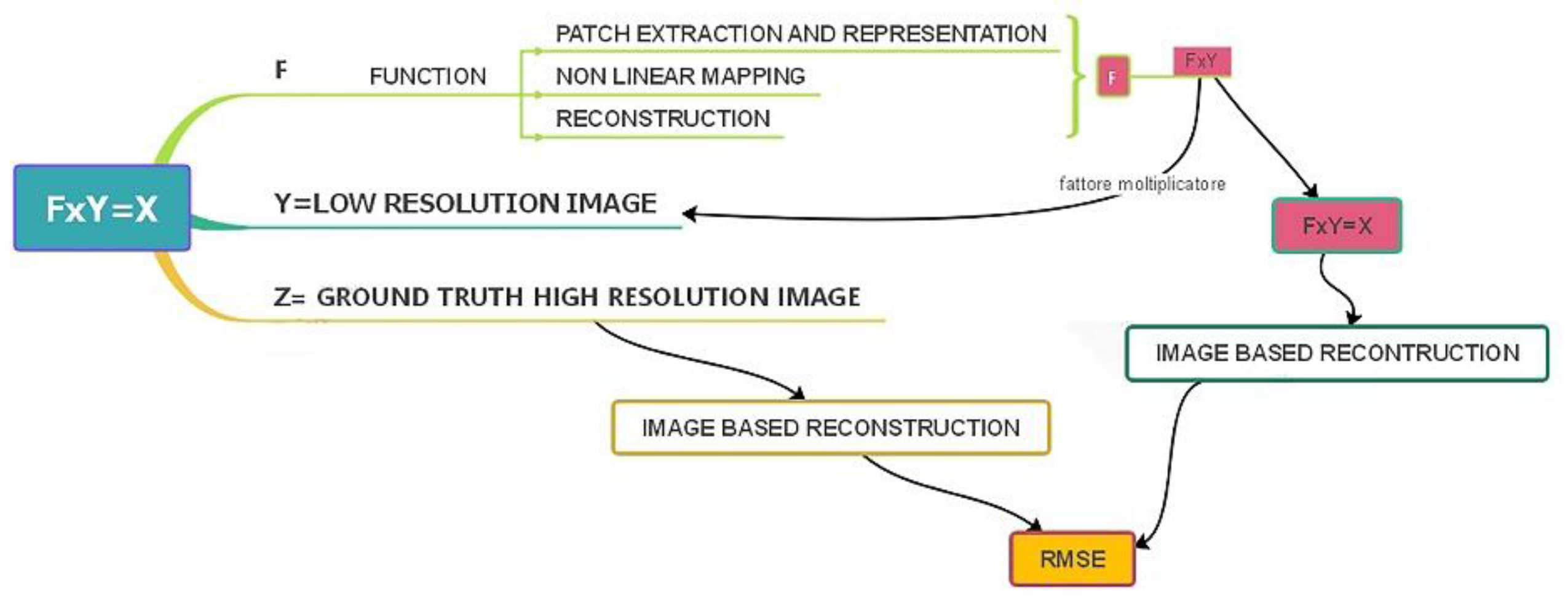
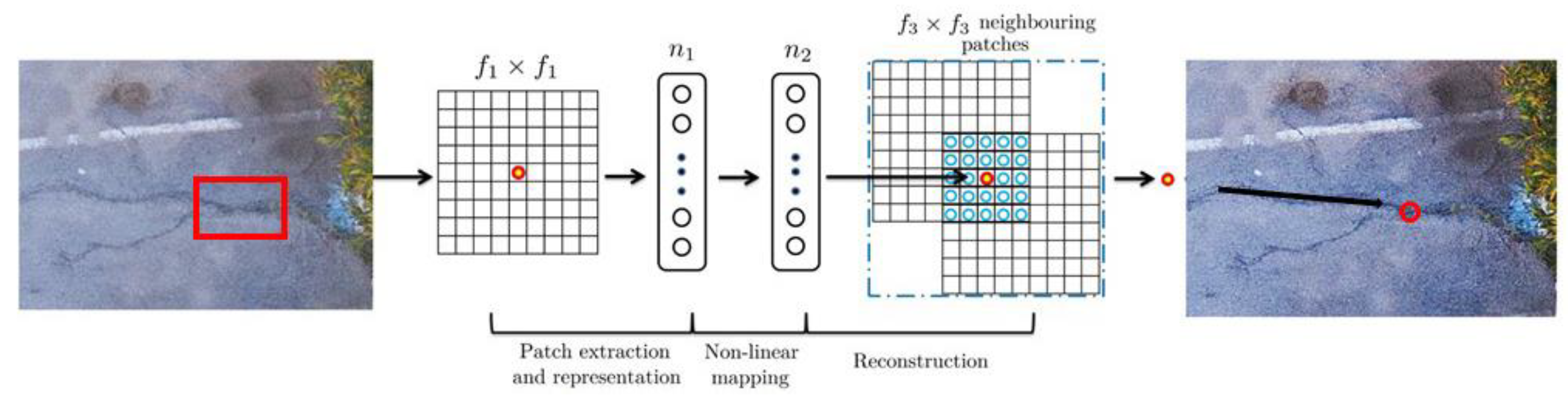
3.1. Image Processing with Super-Revolution
3.2. Photogrammetric Technique for Pavement Distress Detection Using Images Obtained by Drone
4. Investigation
4.1. Road Pavement Monitoring
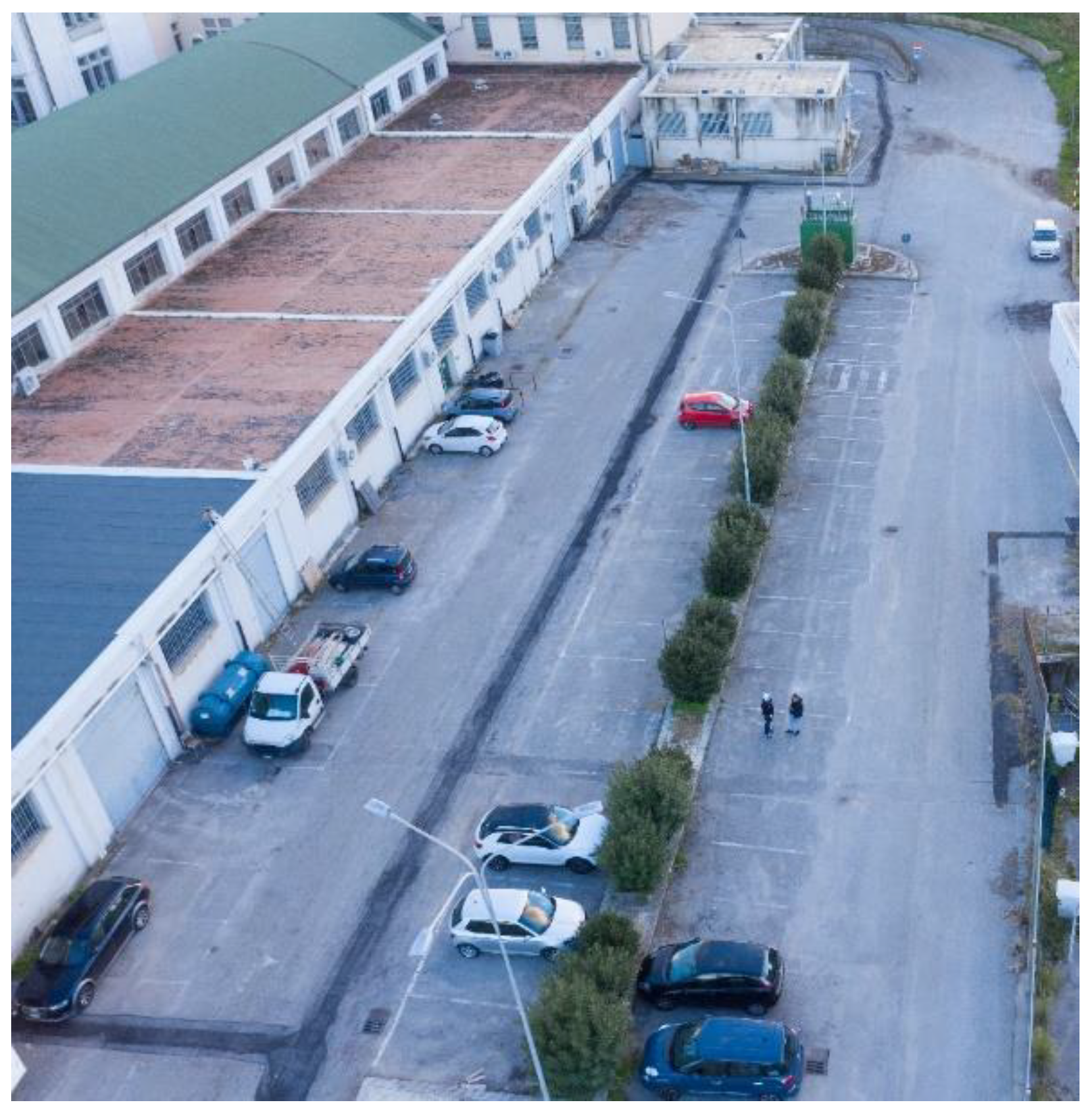
4.2. Case Study
- Video stabilization Movie Solid, a technique named “electronic image stabilization” that cancels out camera shake electronically by cropping an area of an image. Another technique called optical image stabilization is provided to mechanically move the lens to compensate for the shaking of the camera [58]. The huge advantage of electronic image stabilization over optical stabilization is the absence of special hardware requirements, so that is sufficient to work using inexpensive products. The disadvantage is the shrinkage of the effective angle of view due to the image always being cropped.
- Image Stabilization PhotoSolid, that provides sharp images without camera shake or noise [59].Those who have a single-lens reflex camera may know well that camera shake and noise are the counterparts related with image degradation. Cameras, not limited to those of mobile phones, are devices that measure the amount of incident light. In other words, the more light enters a camera, the brighter the image is (and vice versa). When taking photos in a dark scene such as at night, noise is more prevalent than incoming light, which results in noisy images.
- Image Enhancement by AI Based Segmentation and Pixel Filtering Morpho Semantic Filtering™, which is an image enhancement software that implements AI based segmentation and pixel filtering [60].
- Fast AI Inference Engine “SoftNeuro®”, that operates in multiple environments, utilizing learning results that have been obtained through a variety of deep learning frameworks. It’s user-friendly and it doesn’t require any Deep Learning knowledge. SoftNeuro can also import from various frameworks and run fast on several and various architectures. It is both flexible and fast due to the separation of the layer and its execution pattern, which is a concept of routine.
4.3. SfM Reconstructions
5. Results and Discussion
6. Conclusions
Author Contributions
Funding
Institutional Review Board Statement
Informed Consent Statement
Data Availability Statement
Acknowledgments
Conflicts of Interest
References
- Takeda, H.; Farsiu, S.; Milanfar, P. Kernel regression for image processing and reconstruction. IEEE Trans. Image Process. 2007, 16, 349–366. [Google Scholar] [CrossRef] [PubMed] [Green Version]
- Takeda, H.; Milanfar, P.; Protter, M.; Elad, M. Super-resolution without explicit subpixel motion estimation. IEEE Trans. Image Process. 2009, 18, 1958–1975. [Google Scholar] [CrossRef] [PubMed] [Green Version]
- Park, S.C.; Park, M.K.; Kang, M.G. Super-resolution image reconstruction: A technical overview. IEEE Signal Process. Mag. 2003, 20, 21–36. [Google Scholar] [CrossRef] [Green Version]
- Ng, M.K.; Yip, A.M. A fast MAP algorithm for high-resolution image reconstruction with multisensors. Multidimens. Syst. Signal Process. 2001, 12, 143–164. [Google Scholar] [CrossRef]
- Farsiu, S.; Robinson, D.; Elad, M.; Milanfar, P. Robust shift and add approach to superresolution. In Proceedings of the Applications of Digital Image Processing XXVI, San Diego, CA, USA, 3–8 August 2003; Volume 5203. [Google Scholar] [CrossRef]
- Farsiu, S.; Robinson, M.D.; Elad, M.; Milanfar, P. Fast and robust multiframe super resolution. IEEE Trans. Image Process. 2004, 13, 1327–1344. [Google Scholar] [CrossRef]
- Ng, M.K.; Shen, H.; Lam, E.Y.; Zhang, L. A total variation regularization based super-resolution reconstruction algorithm for digital video. EURASIP J. Adv. Signal Process. 2007, 2007, 074585. [Google Scholar] [CrossRef] [Green Version]
- Liu, C.; Sun, D. On bayesian adaptive video super resolution. IEEE Trans. Pattern Anal. Mach. Intell. 2014, 36, 346–360. [Google Scholar] [CrossRef] [Green Version]
- Shen, H.; Zhang, L.; Huang, B.; Li, P. A MAP approach for joint motion estimation, segmentation, and super resolution. IEEE Trans. Image Process. 2007, 16, 479–490. [Google Scholar] [CrossRef]
- Zhang, H.; Zhang, L.; Shen, H. A Blind Super-Resolution Reconstruction Method Considering Image Registration Errors. Int. J. Fuzzy Syst. 2015, 17, 353–364. [Google Scholar] [CrossRef]
- Elad, M.; Feuer, A. Restoration of a single superresolution image from several blurred, noisy, and undersampled measured images. IEEE Trans. Image Process. 1997, 6, 1646–1658. [Google Scholar] [CrossRef] [Green Version]
- Inzerillo, L. SfM Techniques Applied in Bad Lighting and Reflection Conditions: The Case of a Museum Artwork. In Advances in Intelligent Systems and Computing; Springer: Cham, Switzerland, 2020; Volume 943. [Google Scholar] [CrossRef]
- Roberts, R.; Inzerillo, L.; Di Mino, G. Developing a framework for using structure-from-motion techniques for road distress applications. Eur. Transp.-Trasp. Eur. 2020, 77, 1–11. [Google Scholar] [CrossRef]
- Fan, B.; Kong, Q.; Wang, X.; Wang, Z.; Xiang, S.; Pan, C.; Fua, P. A performance evaluation of local features for image-based 3D reconstruction. IEEE Trans. Image Process. 2019, 28, 4774–4789. [Google Scholar] [CrossRef] [PubMed] [Green Version]
- Qiao, G.; Lu, P.; Scaioni, M.; Xu, S.; Tong, X.; Feng, T.; Wu, H.; Chen, W.; Tian, Y.; Wang, W.; et al. Landslide investigation with remote sensing and sensor network: From susceptibility mapping and scaled-down simulation towards in situ sensor network design. Remote Sens. 2013, 5, 4319–4346. [Google Scholar] [CrossRef] [Green Version]
- Barazzetti, L. Planar metric rectification via parallelograms. In Proceedings of the Videometrics, Range Imaging, and Applications XI, Munich, Germany, 23–26 May 2011; Volume 8085. [Google Scholar] [CrossRef]
- Remondino, F.; Nocerino, E.; Toschi, I.; Menna, F. A critical review of automated photogrammetric processing of large datasets. In International Archives of the Photogrammetry, Remote Sensing and Spatial Information Sciences—ISPRS Archives; Copernicus Publications: Göttingen, Germany, 2017; Volume 42. [Google Scholar] [CrossRef] [Green Version]
- Rublee, E.; Rabaud, V.; Konolige, K.; Bradski, G. ORB: An efficient alternative to SIFT or SURF. In Proceedings of the IEEE International Conference on Computer Vision, Barcelona, Spain, 6–13 November 2011. [Google Scholar] [CrossRef]
- Yang, C.Y.; Ma, C.; Yang, M.H. Single-image super-resolution: A benchmark. In Lecture Notes in Computer Science (Including Subseries Lecture Notes in Artificial Intelligence and Lecture Notes in Bioinformatics); Springer Science + Business Media: Berlin, Germany, 2014; Volume 8692 LNCS. [Google Scholar] [CrossRef] [Green Version]
- Glasner, D.; Bagon, S.; Irani, M. Super-resolution from a single image. In Proceedings of the IEEE International Conference on Computer Vision, Kyoto, Japan, 29 September–2 October 2009. [Google Scholar] [CrossRef] [Green Version]
- Kim, K.I.; Kwon, Y. Single-image super-resolution using sparse regression and natural image prior. IEEE Trans. Pattern Anal. Mach. Intell. 2010, 32, 1127–1133. [Google Scholar] [CrossRef]
- Yang, J.; Lin, Z.; Cohen, S. Fast image super-resolution based on in-place example regression. In Proceedings of the IEEE Computer Society Conference on Computer Vision and Pattern Recognition, Portland, OR, USA, 23–28 June 2013. [Google Scholar] [CrossRef] [Green Version]
- Timofte, R.; De, V.; van Gool, L. Anchored neighborhood regression for fast example-based super-resolution. In Proceedings of the IEEE International Conference on Computer Vision, Sydney, Australia, 1–8 December 2013. [Google Scholar] [CrossRef]
- Timofte, R.; De Smet, V.; Van Gool, L. A+: Adjusted anchored neighborhood regression for fast super-resolution. In Lecture Notes in Computer Science (Including Subseries Lecture Notes in Artificial Intelligence and Lecture Notes in Bioinformatics); Springer Science + Business Media: Berlin, Germany, 2015; Volume 9006. [Google Scholar] [CrossRef]
- Ahmadian, K.; Reza-Alikhani, H. reza Single image super-resolution with self-organization neural networks and image laplace gradient operator. Multimed. Tools Appl. 2022, 81, 10607–10630. [Google Scholar] [CrossRef]
- Dong, C.; Loy, C.C.; He, K.; Tang, X. Image Super-Resolution Using Deep Convolutional Networks. IEEE Trans. Pattern Anal. Mach. Intell. 2016, 38, 295–307. [Google Scholar] [CrossRef] [Green Version]
- Burger, H.C.; Schuler, C.J.; Harmeling, S. Image denoising: Can plain neural networks compete with BM3D? In Proceedings of the IEEE Computer Society Conference on Computer Vision and Pattern Recognition, Providence, RI, USA, 16–21 June 2012. [Google Scholar] [CrossRef] [Green Version]
- Schuler, C.J.; Burger, H.C.; Harmeling, S.; Scholkopf, B. A machine learning approach for non-blind image deconvolution. In Proceedings of the IEEE Computer Society Conference on Computer Vision and Pattern Recognition, Portland, OR, USA, 23–28 June 2013; 2013. [Google Scholar]
- Li, X.; Orchard, M.T. New edge-directed interpolation. IEEE Trans. Image Process. 2001, 10, 1521–1527. [Google Scholar] [CrossRef] [Green Version]
- Schulter, S.; Leistner, C.; Bischof, H. Fast and accurate image upscaling with super-resolution forests. In Proceedings of the IEEE Computer Society Conference on Computer Vision and Pattern Recognition, Boston, MA, USA, 7–12 June 2015. [Google Scholar] [CrossRef]
- Xiang, C.; Wang, W.; Deng, L.; Shi, P.; Kong, X. Crack detection algorithm for concrete structures based on super-resolution reconstruction and segmentation network. Autom. Constr. 2022, 140, 104346. [Google Scholar] [CrossRef]
- Liu, Y.; Yeoh, J.K.W.; Chua, D.K.H. Deep Learning–Based Enhancement of Motion Blurred UAV Concrete Crack Images. J. Comput. Civ. Eng. 2020, 34, 04020028. [Google Scholar] [CrossRef]
- Kim, H.; Lee, J.; Ahn, E.; Cho, S.; Shin, M.; Sim, S.H. Concrete crack identification using a UAV incorporating hybrid image processing. Sensors 2017, 17, 2052. [Google Scholar] [CrossRef] [Green Version]
- Ellenberg, A.; Kontsos, A.; Moon, F.; Bartoli, I. Bridge related damage quantification using unmanned aerial vehicle imagery. Struct. Control Health Monit. 2016, 23, 1168–1179. [Google Scholar] [CrossRef]
- Inzerillo, L.; Di Mino, G.; Roberts, R. Image-based 3D reconstruction using traditional and UAV datasets for analysis of road pavement distress. Autom. Constr. 2018, 96, 457–469. [Google Scholar] [CrossRef]
- Bae, H.; Jang, K.; An, Y.K. Deep super resolution crack network (SrcNet) for improving computer vision–based automated crack detectability in in situ bridges. Struct. Health Monit. 2021, 20, 1428–1442. [Google Scholar] [CrossRef]
- Kim, J.; Shim, S.; Cho, G.C. A Study on the Crack Detection Performance for Learning Structure Using Super-Resolution. 2021. Available online: http://www.i-asem.org/publication_conf/asem21/6.TS/3.W5A/4.TS1406_6949.pdf (accessed on 20 May 2022).
- Kondo, Y.; Ukita, N. Crack segmentation for low-resolution images using joint learning with super- resolution. In Proceedings of the MVA 2021—17th International Conference on Machine Vision Applications, Aichi, Japan, 25–27 July 2021. [Google Scholar] [CrossRef]
- Sathya, K.; Sangavi, D.; Sridharshini, P.; Manobharathi, M.; Jayapriya, G. Improved image based super resolution and concrete crack prediction using pre-trained deep learning models. J. Soft Comput. Civ. Eng. 2020, 4, 40–51. [Google Scholar] [CrossRef]
- Jin, Y.; Mishkin, D.; Mishchuk, A.; Matas, J.; Fua, P.; Yi, K.M.; Trulls, E. Image Matching Across Wide Baselines: From Paper to Practice. Int. J. Comput. Vis. 2020, 129, 517–547. [Google Scholar] [CrossRef]
- Low, D.G. Distinctive image features from scale-invariant keypoints. Int. J. Comput. Vis. 2004, 60, 91–110. [Google Scholar] [CrossRef]
- Verdie, Y.; Yi, K.M.; Fua, P.; Lepetit, V. TILDE: A Temporally Invariant Learned DEtector. In Proceedings of the IEEE Computer Society Conference on Computer Vision and Pattern Recognition, Boston, MA, USA, 7–12 June 2015. [Google Scholar] [CrossRef] [Green Version]
- Höhle, J. Oblique aerial images and their use in cultural heritage documentation. Int. Arch. Photogramm. Remote Sens. Spat. Inf. Sci. 2013, XL-5/W2, 349–354. [Google Scholar] [CrossRef] [Green Version]
- Di Mino, G.; Salvo, G.; Noto, S. Pavement management system model using a LCCA—Microsimulation integrated approach. Adv. Transp. Stud. 2014, 1, 101–112. [Google Scholar] [CrossRef]
- Arhin, S.A.; Williams, L.N.; Ribbiso, A.; Anderson, M.F. Predicting Pavement Condition Index Using International Roughness Index in a Dense Urban Area. J. Civ. Eng. Res. 2015, 2015. [Google Scholar]
- Miller, J.S.; Bellinger, W.Y. Distress Identification Manual for the Long-Term Pavement Performance Program. Publ. US Dep. Transp. Fed. Highw. Adm. 2003. [Google Scholar]
- Puan, O.C.; Mustaffar, M.; Ling, T.-C. Automated Pavement Imaging Program (APIP) for Pavement Cracks Classification and Quantification. Malays. J. Civ. Eng. 2007, 19, 1–16. [Google Scholar]
- Chambon, S.; Moliard, J.M. Automatic road pavement assessment with image processing: Review and comparison. Int. J. Geophys. 2011, 2011, 1–20. [Google Scholar] [CrossRef] [Green Version]
- Wang, K.C.P.; Gong, W. Automated pavement distress survey: A review and a new direction. Pavement Eval. Conf. 2002, 21–25. [Google Scholar]
- Wang, K.C.P. Elements of automated survey of pavements and a 3D methodology. J. Mod. Transp. 2011, 19, 51–57. [Google Scholar] [CrossRef] [Green Version]
- Zhang, C. An UAV-based photogrammetric mapping system for road condition assessment. Int. Arch. Photogramm. Remote Sens. Spat. Inf. Sci. 2008, 37, 627–632. [Google Scholar]
- Roberts, R.; Inzerillo, L.; Di Mino, G. Using uav based 3d modelling to provide smart monitoring of road pavement conditions. Information 2020, 11, 568. [Google Scholar] [CrossRef]
- Inzerillo, L.; Roberts, R. 3d image based modelling using google earth imagery for 3d landscape modelling. In Advances in Intelligent Systems and Computing; Springer: Berlin/Heidelberg, Germany, 2019; Volume 919. [Google Scholar] [CrossRef]
- Pan, Y.; Zhang, X.; Cervone, G.; Yang, L. Detection of Asphalt Pavement Potholes and Cracks Based on the Unmanned Aerial Vehicle Multispectral Imagery. IEEE J. Sel. Top. Appl. Earth Obs. Remote Sens. 2018, 11, 3701–3712. [Google Scholar] [CrossRef]
- Kang, D.; Cha, Y.J. Autonomous UAVs for Structural Health Monitoring Using Deep Learning and an Ultrasonic Beacon System with Geo-Tagging. Comput. Civ. Infrastruct. Eng. 2018, 33, 885–902. [Google Scholar] [CrossRef]
- Westoby, M.J.; Brasington, J.; Glasser, N.F.; Hambrey, M.J.; Reynolds, J.M. “Structure-from-Motion” photogrammetry: A low-cost, effective tool for geoscience applications. Geomorphology 2012, 179, 300–314. [Google Scholar] [CrossRef] [Green Version]
- Shen, T.; Luo, Z.; Zhou, L.; Zhang, R.; Zhu, S.; Fang, T.; Quan, L. Matchable Image Retrieval by Learning from Surface Reconstruction. In Lecture Notes in Computer Science (Including Subseries Lecture Notes in Artificial Intelligence and Lecture Notes in Bioinformatics); Springer Science + Business Media: Berlin/Heidelberg, Germany, 2019; Volume 11361 LNCS. [Google Scholar] [CrossRef] [Green Version]
- Luo, Z.; Zhou, L.; Bai, X.; Chen, H.; Zhang, J.; Yao, Y.; Li, S.; Fang, T.; Quan, L. ASLFEaT: Learning local features of accurate shape and localization. In Proceedings of the Proceedings of the IEEE Computer Society Conference on Computer Vision and Pattern Recognition, Seattle, WA, USA, 13–19 June 2020. [Google Scholar] [CrossRef]
- Schönberger, J.L.; Hardmeier, H.; Sattler, T.; Pollefeys, M. Comparative evaluation of hand-crafted and learned local features. In Proceedings of the 30th IEEE Conference on Computer Vision and Pattern Recognition, CVPR 2017, Honolulu, HI, USA, 21–26 July 2017; Volume 2017-January. [Google Scholar] [CrossRef]
- Moulon, P.; Monasse, P.; Perrot, R.; Marlet, R. OpenMVG: Open multiple view geometry. In Lecture Notes in Computer Science (Including Subseries Lecture Notes in Artificial Intelligence and Lecture Notes in Bioinformatics); Springer Science + Business Media: Berlin/Heidelberg, Germany, 2017; Volume 10214 LNCS. [Google Scholar] [CrossRef] [Green Version]
- Freedman, G.; Fattal, R. Image and video upscaling from local self-examples. ACM Trans. Graph. 2011, 30, 1–11. [Google Scholar] [CrossRef] [Green Version]
- Fedele, R.; Scaioni, M.; Barazzetti, L.; Rosati, G.; Biolzi, L. Delamination tests on CFRP-reinforced masonry pillars: Optical monitoring and mechanical modeling. Cem. Concr. Compos. 2014, 45, 243–254. [Google Scholar] [CrossRef]
- Jancosek, M.; Pajdla, T. Multi-view reconstruction preserving weakly-supported surfaces. In Proceedings of the IEEE Computer Society Conference on Computer Vision and Pattern Recognition, Colorado Springs, CO, USA, 20–25 June 2011. [Google Scholar] [CrossRef]
- Gruen, A. Development and Status of Image Matching in Photogrammetry. Photogramm. Rec. 2012, 27, 36–57. [Google Scholar] [CrossRef]
- Barazzetti, L.; Scaioni, M. Crack measurement: Development, testing and applications of an automatic image-based algorithm. ISPRS J. Photogramm. Remote Sens. 2009, 64, 285–296. [Google Scholar] [CrossRef]
- Barazzetti, L.; Scaioni, M. Development and implementation of image-based algorithms for measurement of deformations in material testing. Sensors 2010, 10, 7469–7495. [Google Scholar] [CrossRef] [Green Version]
- Fraser, C.S. Photogrammetric measurement to one part in a million. Photogramm. Eng. Remote Sens. 1992, 58, 305–310. [Google Scholar]
- Fraser, C.S. Automatic camera calibration in close range photogrammetry. Photogramm. Eng. Remote Sens. 2013, 79, 381–388. [Google Scholar] [CrossRef] [Green Version]
- Stathopoulou, E.K.; Welponer, M.; Remondino, F. Open-source image-based 3D reconstruction pipelines: Review, comparison and evaluation. In International Archives of the Photogrammetry, Remote Sensing and Spatial Information Sciences—ISPRS Archives; Copernicus Publications: Göttingen, Germany, 2019; Volume 42. [Google Scholar] [CrossRef] [Green Version]
- Niederheiser, R.; Mokroš, M.; Lange, J.; Petschko, H.; Prasicek, G.; Elberink, S.O. Deriving 3d point clouds from terrestrial photographs—Comparison of different sensors and software. Int. Arch. Photogramm. Remote Sens. Spat. Inf. Sci. 2016, XLI-B5, 685–692. [Google Scholar] [CrossRef] [Green Version]
- Di Filippo, A.; Villecco, F.; Cappetti, N.; Barba, S. A Methodological Proposal for the Comparison of 3D Photogrammetric Models. In Lecture Notes in Mechanical Engineering; Springer: Berlin/Heidelberg, Germany, 2022. [Google Scholar] [CrossRef]
- Barba, S.; Ferreyra, C.; Cotella, V.A.; di Filippo, A.; Amalfitano, S. A SLAM Integrated Approach for Digital Heritage Documentation. In Lecture Notes in Computer Science (Including Subseries Lecture Notes in Artificial Intelligence and Lecture Notes in Bioinformatics); Springer Science + Business Media: Berlin/Heidelberg, Germany, 2021; Volume 12794 LNCS. [Google Scholar] [CrossRef]
- Morena, S.; Molero Alonso, B.; Barrera-Vera, J.A.; Barba, S. As-built graphic documentation of the Monumento a la Tolerancia. Validation of low-cost survey techniques. EGE-Expresión Gráfica Edif. 2020, 98–114. [Google Scholar] [CrossRef]
- Fukozono, T. Recent studies on time prediction of slope failure. Landslide News 1990, 4, 9–12. [Google Scholar]


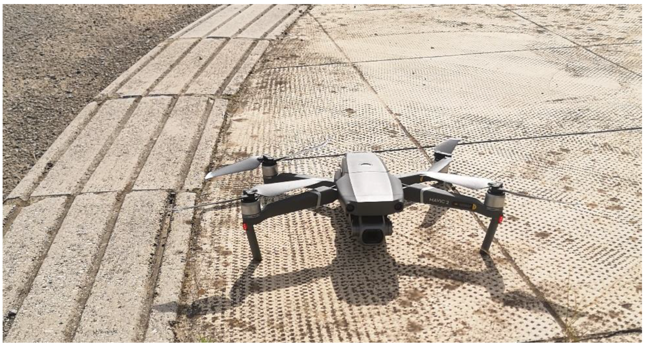
| Device | DJI Mavic 2 Pro | Camera 1 |
|---|---|---|
| Camera resolution (megapixel) | 20 | 20.9 |
| Image size (pixel) | 5568 × 3648 | 5568 × 3712 |
| Sensor size (mm) Focal length (35 mm eq.) | 13.2 × 8.8 28 | 23.5 × 17.5 24 |
| ISO | 200 | 100 |
| Shutter speed | 1/60 to 1/125 | 1/250 |
| Aperture | f/5.6 | f/8 |
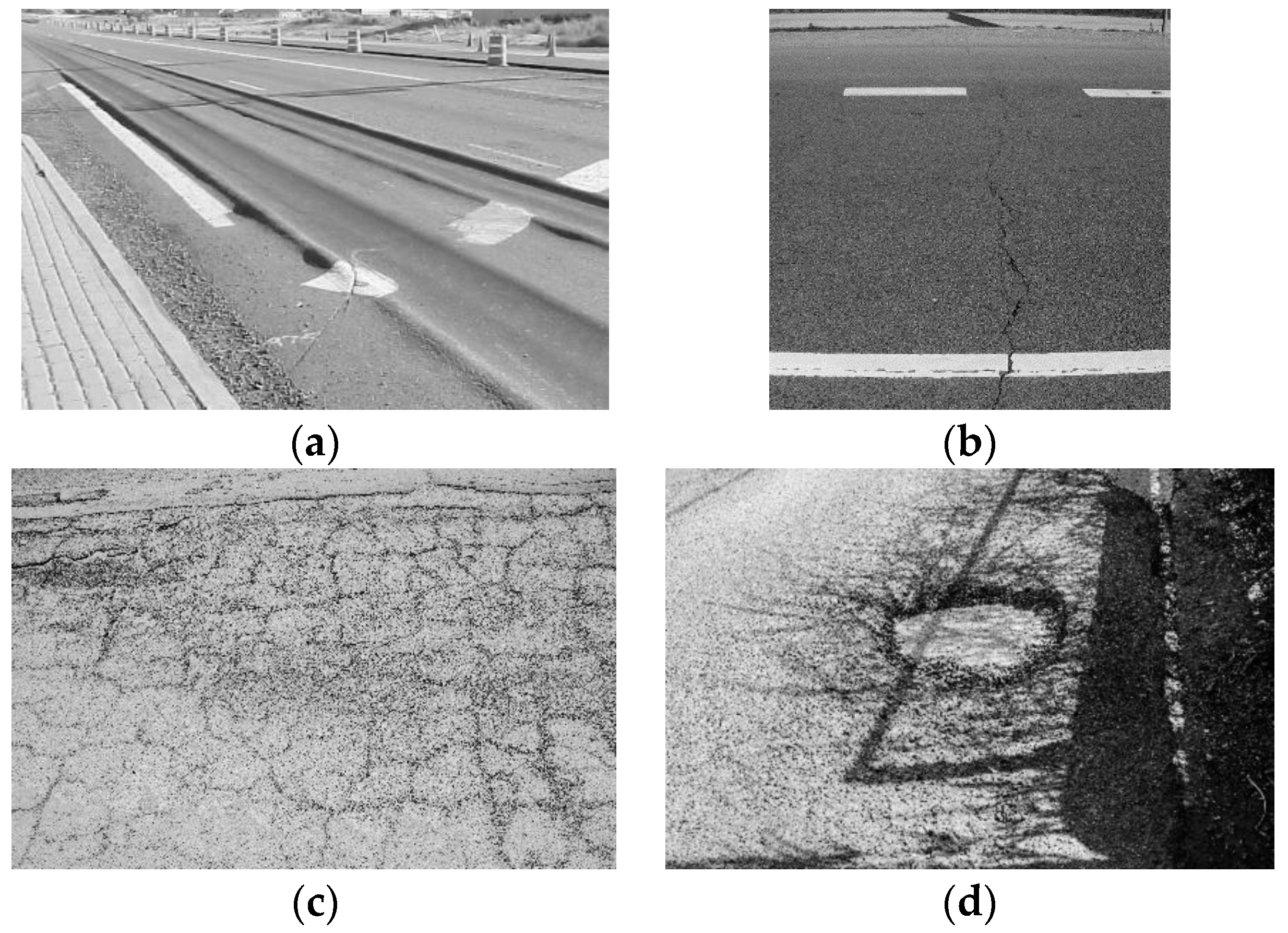
| Distress | Indicator | Severity Levels 1,2 |
|---|---|---|
| Block Cracking | Crack Width (mm) | 3–19 mm |
| Transverse Cracking | Crack Width (mm) | 3–19 mm |
| Potholes Rutting | Depth (mm) Depth (mm) | 25–50 mm >12 mm |
| Number of Images: | 20 | Camera Stations: | 20 |
|---|---|---|---|
| Flying altitude | 49.7 m | Tie points: | 11.985 |
| Ground resolution: | 1.24 cm/pix | Projections: | 36.698 |
| Coverage area: | 5.01 × 10³ m2 | Reprojection error: | 0.823 pix |
| Value | Error | F | Cx | Cy | K1 | K2 | K3 | P1 | P2 | |
|---|---|---|---|---|---|---|---|---|---|---|
| F | 4295.9 | 2.1 | 1.00 | −0.32 | −1.00 | −0.18 | 0.22 | −0.28 | −0.09 | 0.06 |
| Cx | 53.9991 | 0.24 | 1.00 | 0.33 | −0.04 | 0.00 | 0.04 | 0.94 | −0.11 | |
| Cy | 65.7928 | 3.1 | 1.00 | 0.15 | −0.19 | 0.25 | 0.10 | −0.07 | ||
| K1 | −0.015095 | 0.00022 | 1.00 | −0.97 | 0.91 | −0.05 | −0.01 | |||
| K2 | 0.030799 | 0.00075 | 1.00 | −0.98 | 0.04 | 0.05 | ||||
| K3 | −0.031978 | 0.00083 | 1.00 | −0.01 | −0.05 | |||||
| P1 | 0.003128 | 1.9 × 10⁻⁵ | 1.00 | −0.03 | ||||||
| P2 | −0.00052 | 1.3 × 10⁻⁵ | 1.00 |
| Number of Images: | 20 | Camera Stations: | 20 |
|---|---|---|---|
| Flying altitude | 51.6 m | Tie points: | 19.855 |
| Ground resolution: | 7.11 mm/pix | Projections: | 38.519 |
| Coverage area: | 4.77 × 10³ m2 | Reprojection error: | 1.05 pix |
| Value | Error | F | Cx | Cy | K1 | K2 | K3 | P1 | P2 | |
|---|---|---|---|---|---|---|---|---|---|---|
| F | 6950.26 | 2.6 | 1.00 | −0.29 | −1.00 | −0.18 | 0.21 | −0.26 | −0.04 | 0.07 |
| Cx | 85.7596 | 0.26 | 1.00 | 0.30 | −0.07 | 0.04 | 0.00 | 0.94 | −0.13 | |
| Cy | 97.1246 | 3.8 | 1.00 | 0.14 | −0.18 | 0.24 | 0.05 | −0.07 | ||
| K1 | −0.0151 | 0.00015 | 1.00 | −0.96 | 0.91 | −0.09 | −0.03 | |||
| K2 | 0.029503 | 0.00054 | 1.00 | −0.98 | 0.08 | 0.04 | ||||
| K3 | −0.02972 | 0.0006 | 1.00 | −0.05 | −0.04 | |||||
| P1 | 0.003039 | 1.3 × 10⁻⁵ | 1.00 | −0.04 | ||||||
| P2 | −0.00049 | 9.3 × 10⁻⁶ | 1.00 |
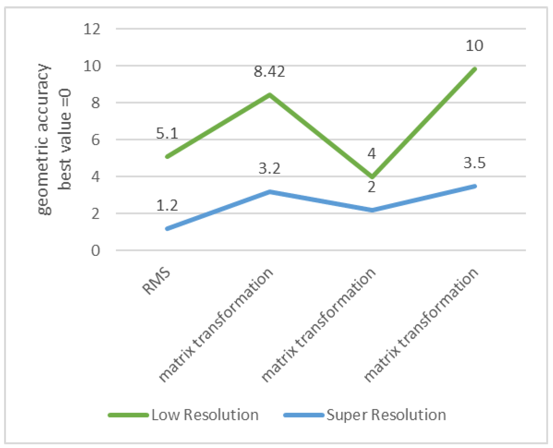
| X Error (cm) | Y Error (cm) | Z Error (cm) | XY Error (cm) | Tot. Error (cm) |
|---|---|---|---|---|
| 5.135658 1 | 8.424 1 | 7.5754 1 | 9.8569 1 | 12.0556 1 |
| 1.22132 2 | 3.8425 2 | 2.3766 2 | 4.7335 2 | 5.6146 2 |
Publisher’s Note: MDPI stays neutral with regard to jurisdictional claims in published maps and institutional affiliations. |
© 2022 by the authors. Licensee MDPI, Basel, Switzerland. This article is an open access article distributed under the terms and conditions of the Creative Commons Attribution (CC BY) license (https://creativecommons.org/licenses/by/4.0/).
Share and Cite
Inzerillo, L.; Acuto, F.; Di Mino, G.; Uddin, M.Z. Super-Resolution Images Methodology Applied to UAV Datasets to Road Pavement Monitoring. Drones 2022, 6, 171. https://doi.org/10.3390/drones6070171
Inzerillo L, Acuto F, Di Mino G, Uddin MZ. Super-Resolution Images Methodology Applied to UAV Datasets to Road Pavement Monitoring. Drones. 2022; 6(7):171. https://doi.org/10.3390/drones6070171
Chicago/Turabian StyleInzerillo, Laura, Francesco Acuto, Gaetano Di Mino, and Mohammed Zeeshan Uddin. 2022. "Super-Resolution Images Methodology Applied to UAV Datasets to Road Pavement Monitoring" Drones 6, no. 7: 171. https://doi.org/10.3390/drones6070171
APA StyleInzerillo, L., Acuto, F., Di Mino, G., & Uddin, M. Z. (2022). Super-Resolution Images Methodology Applied to UAV Datasets to Road Pavement Monitoring. Drones, 6(7), 171. https://doi.org/10.3390/drones6070171