1. Introduction
Recent technological developments have made autonomous and unmanned maritime vehicles realistic alternatives to traditional vessel-based survey and monitoring systems [
1]. Potential benefits of using unmanned maritime vehicles include reduced operational costs, improved safety and reliability, longer monitoring durations and mission repeatability. Two important vehicle classes are unmanned surface vehicles (USVs) and autonomous underwater vehicles (AUVs). Teams consisting of collaborating vehicles of both types can be used in applications that include safety and rescue missions, environmental disaster assessment, underwater geology, marine archeology, military survey, and detection and monitoring of marine fauna [
2]. The latter area includes population surveys, migration tracking and vocal animal monitoring [
3]. Some applications of AUVs and USVs for ocean wildlife monitoring and mapping are given in [
4,
5].
In this paper, we address the problem of a USV and an AUV navigating collaboratively to exchange data at close range. Under the considered scenario, the AUV collects some information in the submerged mode, e.g., from a seabed survey in a disaster assessment application, or intelligence information in military applications, with remote supervision from a USV. It must periodically rendezvous with the USV to offload a summary that the USV can transmit for operator inspection. The AUV could come to the surface for data transmission via one or more terrestrial communication systems (e.g., Wi-Fi), but in doing so it would lose most of its control authority while being exposed to rapidly changing sea surface conditions and the risk of collision with vessels [
6]. We leave this difficult problem for future investigation and consider a different scenario; transmission of data while the AUV remains submerged, noting however that underwater data exchange using acoustic modems is notoriously slow, unreliable and range-dependent [
7]. We are therefore motivated to find a solution that minimises the separation between the AUV and the USV to maximise the data transmission rate, while remaining sufficiently far apart to avoid the risk of collision with the supervising USV if the AUV is unexpectedly forced to come to the surface.
We state a constrained optimal control problem in which the AUV and USV navigate collaboratively to maximise the amount of data transmitted while keeping the probability of collision between them sufficiently small. We prove that the optimal solution to this problem is delivered by a navigation algorithm belonging to the class of sliding mode control laws [
8,
9].
Various problems of controlling multi-vehicle systems to achieve a certain objective are referred to as cooperative control; see, e.g., [
10,
11]. Thus, the problem studied in this paper falls into the domain of collaborative control.
The remainder of the paper is organised as follows. In
Section 2, we give a brief survey of relevant publications in the field. In
Section 3, we present the system model and state the problem under investigation. In
Section 4, we present the proposed navigation law together with its theoretical analysis. Computer simulations illustrating the developed navigation method are conducted in
Section 5 to show the performance of the proposed algorithm. Finally, a brief conclusion and possible directions for future research are given in
Section 6.
2. Related Work
In recent years, research publications on using collaborating autonomous unmanned vehicles in monitoring applications have concentrated on unmanned aerial vehicles (UAVs); in particular, a review of recent results on deployment and navigation of teams of collaborating UAVs for surveillance can be found in the survey paper [
12].
Research concerning autonomous marine vehicles working in collaboration has been more limited, possibly due to the relatively high cost associated with acquiring and operating such systems. However, the literature associated with this field is increasing.
Recent reviews of path planning for AUVs can be found in [
13,
14,
15]. Teams of collaborating AUVs are studied in [
16], where issues of navigation, localisation and underwater communication are analysed and various types of missions for AUV teams are discussed. Another approach for cooperative navigation of teams of AUVs was developed in [
17].
Navigation of USVs is studied in [
18]. The paper [
19] addresses navigation of collaborating USVs for intruder interception on a marine region boundary. The publication [
11] addresses a problem of path planning for a team of collaborating vehicles in marine safety and rescue missions.
Collision avoidance problems for various types of unmanned vehicles have attracted a lot of attention in recent decades; see, e.g., the survey papers [
20,
21]. Most of this research has concentrated on two-dimensional problems, usually for ground mobile robots [
22]; however, many proposed collision avoidance algorithms may be extended to obstacle avoidance for USVs; see, e.g., [
23,
24]. Three-dimensional collision avoidance problems are also attracting attention; see, e.g., [
25,
26,
27,
28]. Most of the research on 3D collision avoidance concentrates on UAV navigation; however, many developed methods can be extended to collision-free navigation of AUVs [
29,
30]. Furthermore, some machine-learning-based approaches to AUV path planning with obstacle avoidance were recently proposed in [
31,
32].
At present, there are relatively few examples of systems involving collaborating AUVs and USVs [
33,
34], although Ocean Infinity used USV-AUV teams extensively for search operations connected with the disappearance of Malaysian Airlines flight MH370 [
35]. This is a quite novel research area. The paper [
6] addresses a navigation problem for an AUV-USV system for ocean sampling, environmental monitoring and providing real-time pollution measurement data. The paper [
36] develops a method for a team of collaborating robots to sample primary production in the ocean. Furthermore, [
37] addresses a control problem for a USV that deploys a remotely operated vehicle (ROV); however, unlike the current paper, [
37] does not study a scenario with acoustic underwater communication, because the USV and the ROV are connected by an underwater cable. Finally, a problem involving collaboration between a UAV and an AUV was studied in [
38].
3. Problem Statement
We consider an autonomous underwater vehicle (AUV), submerged in a 3D halfspace. Let
be the AUV’s coordinates at time
t, where
and
are the coordinates in the horizontal plane parallel to the ground and
is the depth. We consider the following well-known model for the motion of the AUV:
Here
is the heading of the AUV;
,
and
are its linear horizontal, angular and vertical speeds, respectively; and
and
are given positive constants indicating the maximum linear, angular and vertical speeds, respectively. The linear horizontal speed
, angular speed
and the vertical speed
are the control inputs of the system (
1). Furthermore, the AUV depth
should satisfy the constraints:
where
are given constants. Furthermore, there is a moving unmanned surface vehicle (USV), with motion described by the following equations:
Here is the heading of the USV; and are its linear horizontal and angular speeds, respectively; and are given positive constants indicating the maximum linear and angular speeds of the USV.
Typically, AUVs are battery-powered devices that move slowly—most cruise at between 1.5 and 2 ms and have limited acceleration. In contrast, USVs that are used for supervision typically move and accelerate more quickly and have much better situational awareness. Therefore, we assume that it is appropriate to minimise the requirement for the AUV to manoeuvre; the USV is responsible for controlling its position relative to the AUV at all times.
The AUV collects some information while submerged, which it must periodically transmit to the USV. The USV (or surface vessel under autopilot control) informs the AUV that it is ready to exchange acoustic messages. The submerged AUV comes sufficiently close to the USV for acoustic communication and maintains a steady course, speed and depth.
In this scenario, we assume that at least one and potentially two sets of acoustic modems are transmitting data between the USV and the AUV: medium-range acoustic modems that transmit control instructions and telemetry and optionally short-range acoustic modems operating in a higher frequency band that transmit data at a higher rate. We assume that telemetry and control messages can be short and infrequent, but data transmission is an extended operation that is sensitive to the separation and relative position of the two vehicles; thus, it is advantageous that they maintain a constant separation and mutual orientation while data transmission is underway.
Because the telemetry channel has very low bandwidth, we assume that the AUV periodically transmits its state information to the USV, but it relies on the USV to manoeuvre safely during data transmission and does not monitor state transmissions from the USV. Thus, the USV can maintain an estimate of the coordinates, speed and heading of the AUV, but the AUV does not know, or does not react to, the state of the USV.
In this paper, we seek to develop an optimal strategy for reliably transmitting the data from the submerged AUV to the USV while avoiding collisions between the vehicles.
We consider a time interval
. Let
be a given integer. We divide
into
N equal intervals of length
. At any time instant
, the AUV with probability
p transmits some messages to the USV using an acoustic communication system. Here
p is a given constant such that
. The probability of successful reception of the message by the USV is described by a given decreasing function
such that
, where
is the distance between the AUV and the USV at time
t. Here we consider the problem of missed reception as the probability of successful reception is
, where
is the distance between the autonomous vehicles. Since
for all
, with some non-zero probability the signal will be missed. Moreover, the USV needs to avoid collision with the AUV. Let
be given constants. We assume that to avoid collisions, the distance
between the AUV and the USV at time
t should always satisfy the constraint:
Furthermore, we assume that any distance
is totally safe; however, it is desired that the USV would be at distances between
and
from the AUV in as short time as possible to minimise the risk of errors in mutual position estimates causing a collision between the USV and the AUV. More precisely, we introduce some function
defined for
and decreasing such that
for all
. We need to satisfy the following requirement:
where
is a given small probability, and the integral in (
5) describes the probability of collision between the vehicles at a distance between
and
over the time interval
.
Furthermore, the motion of the AUV and the USV should satisfy the following safety requirement that guarantees smooth enough changes of the distance between the vehicles:
where
is a given constant.
Now, let be the number of messages from the AUV successfully received by the USV over the time interval , and let denote the mathematical expectation of a random variable.
Problem Statement: To construct control inputs
for the AUV (
1) and the USV (
3) so that the optimal control problem
subject to the constraints (
2), (
4)–(
6).
4. Navigation Law
We propose the following navigation law: at time
, the USV selects some heading
and follows in this direction using the following sliding mode controller:
where
is the sign function defined as follows:
Furthermore, the USV transmits this direction
to the AUV, which uses an analogous controller:
It is obvious that after some time
, both vehicles will have headings
for all
with any control inputs
. Notice that the controllers (
8) and (
10) belong to the class of sliding mode controllers [
8] or switched controllers [
39].
Let
and
be given positive integers. We consider the following class of piecewise constant functions
that can change values at discrete time instants
where
Moreover,
takes values only in the discrete set of
numbers:
Now, we propose the following optimisation scheme. We take all possible piecewise constant functions
with values from the set (
12) changing values at discrete time instants
and introduce the functions
for all
.
Furthermore, we consider only pairs
such that
satisfies the constraints (
4) and (
5). Let
denote the set of all such pairs. Now, we select
such that
delivers the maximum of the cost function
over all
.
In other words, we select the function
using the brute force method, i.e., complete search in the set of all possible piecewise constant functions
taking values from the set (
12). Note that at any discrete time instant, there are
options of values of
. Then, for
instants, there are
possible functions
. However, in practice, as we only employ functions
that meet the constraints (
4) and (
5), we get a much smaller number of elements in the set
, which greatly reduces the computational complexity of this optimisation scheme.
Now we consider the following navigation law over :
NL1: The AUV chooses an arbitrary control input
, where
some given constant, and the control input
is defined by (
10). Furthermore, the AUV chooses the control input
defined by
.
NL2: The USV applies the control inputs
defined by
where
is the angle between the heading
and the line connecting the current positions of the AUV and the USV. Furthermore, the control input
is defined by (
8).
Our main theoretical result requires some assumptions.
Assumption A1. The following inequalities hold: (2) and (4) hold at time . Assumption A2. The following inequality holds: Theorem 1. Consider the optimisation problem (7) for the AUV (1) and the USV (3) subject to the constraints (2), (4)–(6). As and , the value of the cost function (7) delivered by the navigation law NL1, NL2 converges to the global supremum in (7). Proof. Under the navigation law NL1, NL2, the AUV is moving in a plane that is parallel to the surface, so
is constant; therefore, Assumption A1 implies that the constraint (
2) always holds. Furthermore, under the navigation law NL1, NL2, the AUV and the USV are moving along two parallel straight lines with the direction
. Since the AUV and the USV are moving in the direction
, it follows from (
8) and (
10) that
for all
. This implies that the derivative
of the distance
between the AUV and the USV satisfies
see, e.g., [
22]. Moreover, (
19) implies that if the USV’s control input
is defined by (
15) with some function
, then
where
is defined by (
13) with
. Furthermore, in this case, the cost function (
7) is equal to the function (
14). It is also obvious that the cost function (
7) and the constraints (
4)–(
6) depend only on
. Therefore, the navigation law NL1, NL2 delivers the maximum in the optimisation problem (
7) subject to the constraints (
2), (
4)–(
6) in the class of control inputs such that
is piecewise constant with constant values on each of
intervals from the class (
12). Any
can be approximated with an arbitrary small precision by piecewise constant functions. Therefore, we can build a sequence of
from the above class for which the cost function (
14) converges to the global supremum in (
7) as
and
. Finally, Assumption A2 obviously guarantees that the control input
of the AUV defined by (
15) satisfies the constraint
. □
Remark 1. It should be pointed out that the proposed algorithm produces an asymptotically accurate approximation of the global optimum in the sense that as the parameters and are large enough, the obtained trajectories converge to the optimum.
Remark 2. A physical interpretation on the inequalities (A1) from Assumption A1 is quite clear. They guarantee at the initial time that the AUV satisfies the depth constraint (2) and the safety constraint (4). Furthermore, a physical interpretation of the inequality (18) from Assumption A2 is that the maximum linear speed of the USV is larger than the current linear speed of the AUV with some margin that allows the USV to perform its manoeuvre as the USV is responsible for controlling its position relative to the AUV. Notice also that Assumption A2 is an assumption of a technical nature guaranteeing that the control input of the USV defined by the navigation law NL1, NL2 satisfies the constraint . The requirement (18) is quite conservative, and in practice, the constraint often holds even when Assumption A2 is not satisfied. Remark 3. Notice that in practice, due to lack of communication and/or loss of data transmitted from the AUV to the USV, the USV would model the position of the AUV with a robust Kalman filter [40], algorithms of state estimation over communication channels [41] or similar techniques as uncertainty would increase whenever there was a significant period when the USV did not receive a state transmission from the AUV. However, we do not study this issue in this paper. 5. Illustrative Examples and Computer Simulations
In this section, we present results of computer simulation that illustrate the performance of the navigation NL1, NL2. Simulations are performed in MATLAB software. We take times
s and
s. Then we apply the navigation law NL1, NL2 ten times over the time intervals [20 s, 70 s], [70 s, 120 s], …, [470 s, 520 s]. The values of the parameters used in simulations are
,
,
,
m,
m,
ms
,
ms
,
,
s,
ms
,
rads
,
m,
m,
ms
,
ms
,
rads
,
s,
and
. Initially, the AUV and USV are at different coordinates and have different headings. The position of the AUV is
with initial heading
, while the USV is at
with initial heading
. The decreasing function used for the Equation (
5) is defined as
and the cost function for the Equation (
14) is described as
. The simulation runs for 520 s. Initially, in the first 20 s, both vehicles steer the same course
. Thereafter, in the next 500 s, the AUV sends data to the USV. This interval is split into 10 equal intervals of 50 s each. The navigation algorithm is tested in three different scenarios as follows. Except where indicated, the parameters and initial conditions remain the same.
Note that the probability function
that we have assumed does not accurately reflect the performance of any particular acoustic or other underwater communications device, but the control law is not critically dependent on its particular form, so long as it is monotonically decreasing. Better models of particular modems could be included through the use of an underwater communication simulation system such as AquaSim NG (see, for example, [
42]). The same is true for the function
, as the proposed control law is not critically dependent on its particular form, so long as it is monotonically decreasing.
5.1. Scenario I
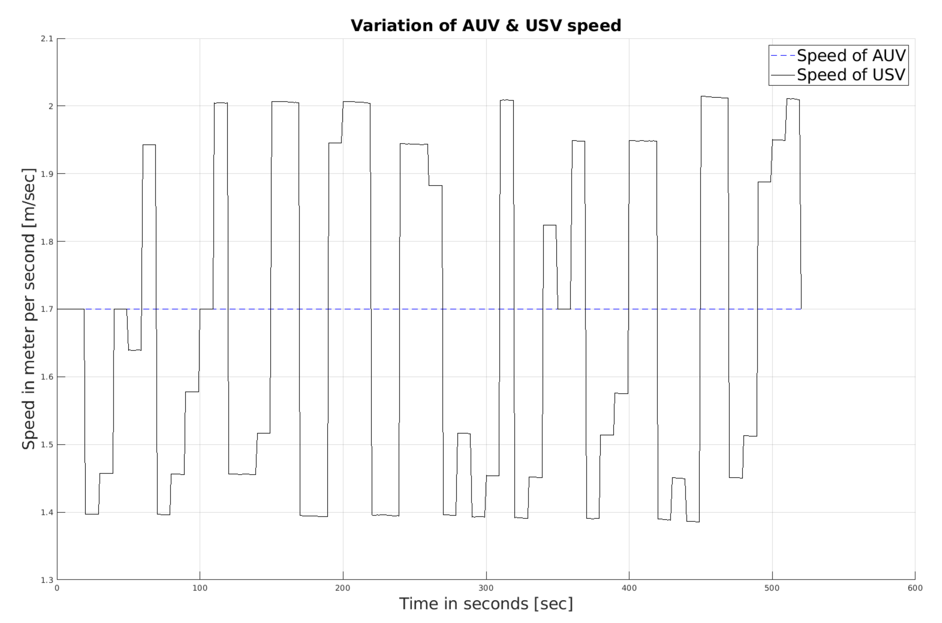
The AUV is travelling at a constant speed
ms
, and the USV transmits a new direction angle
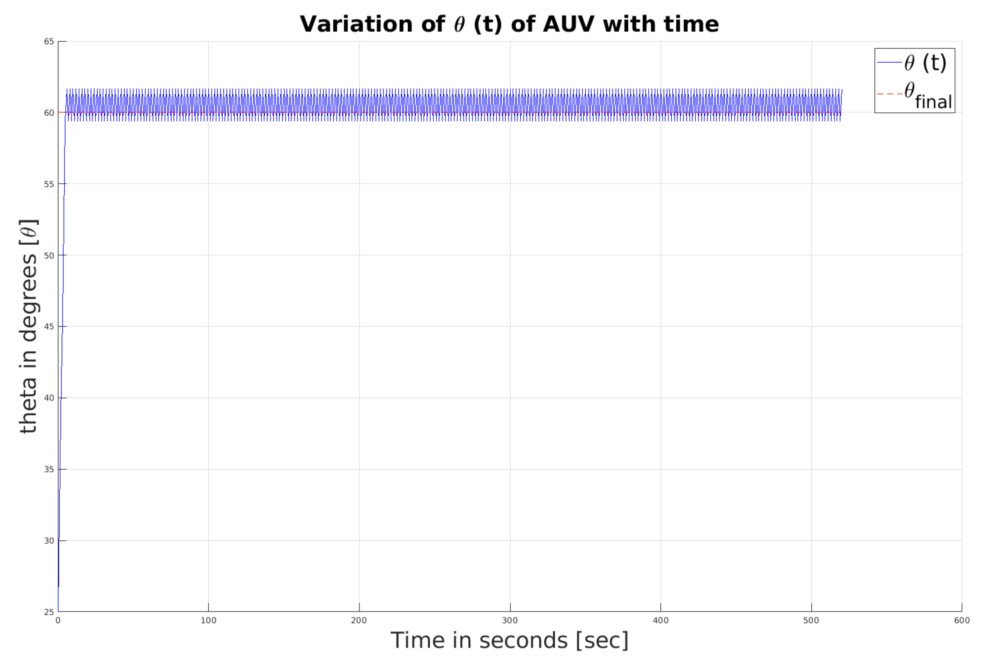
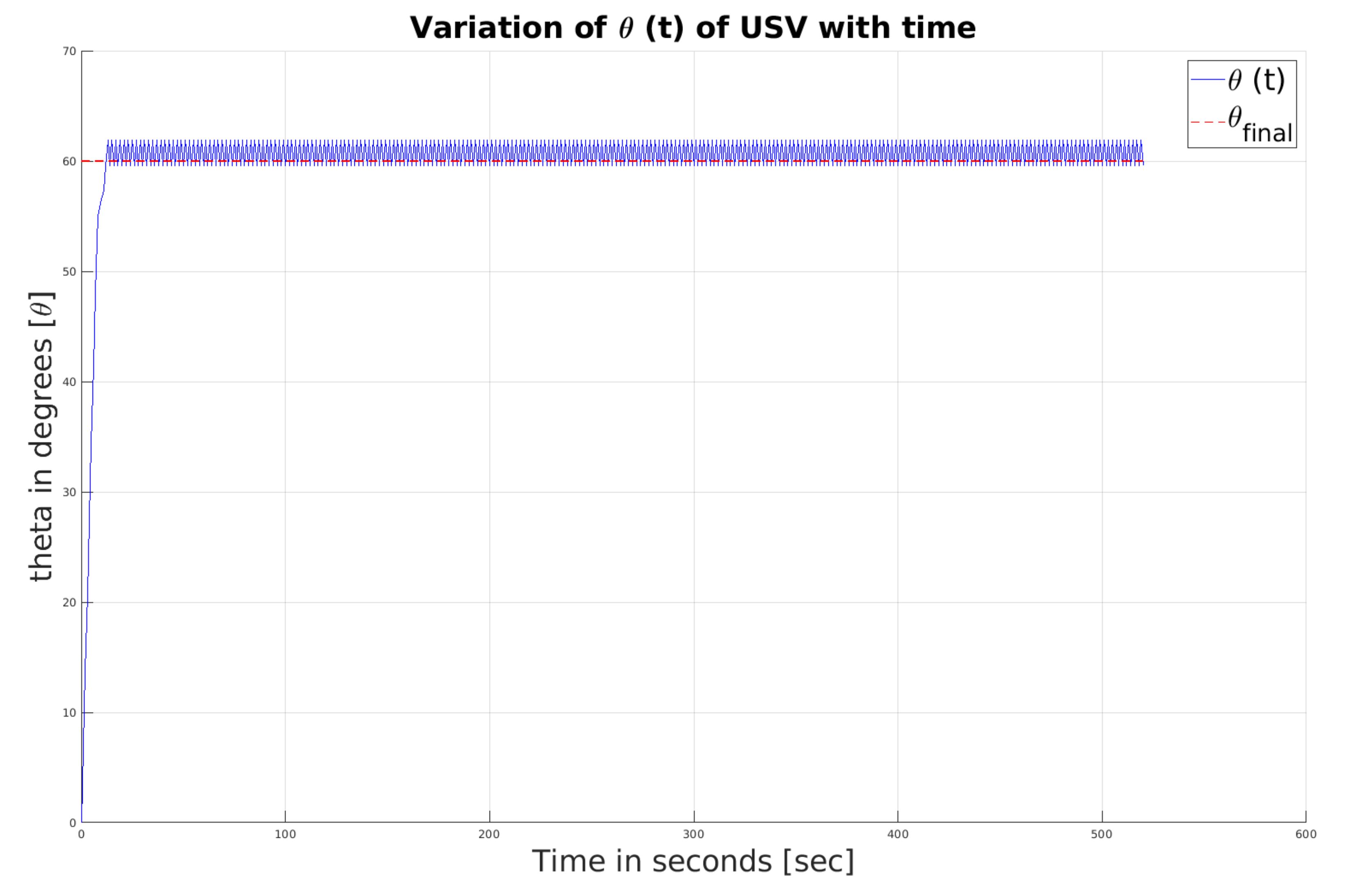
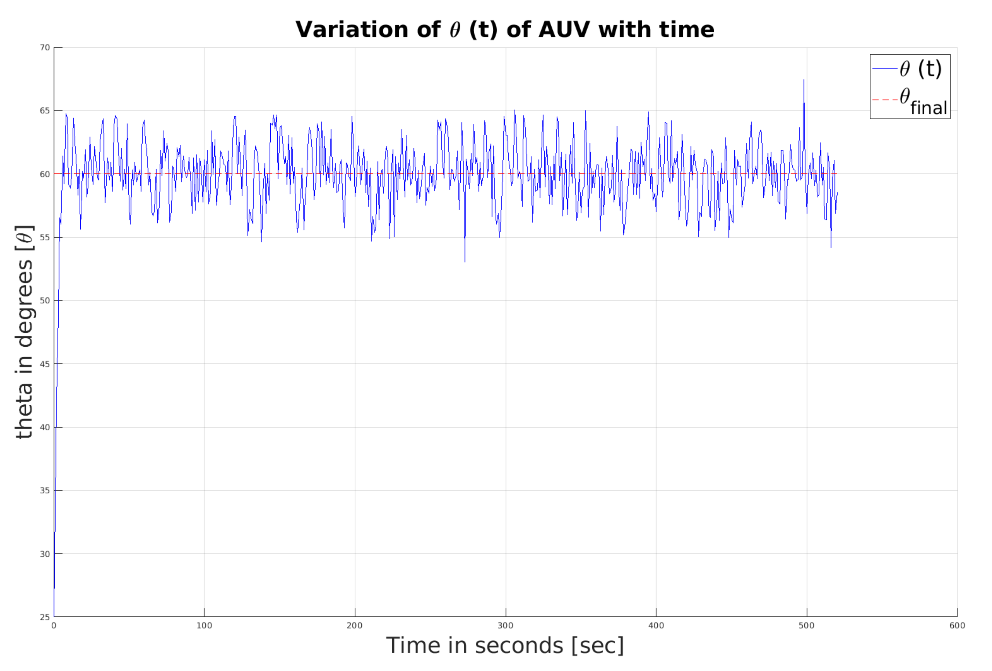
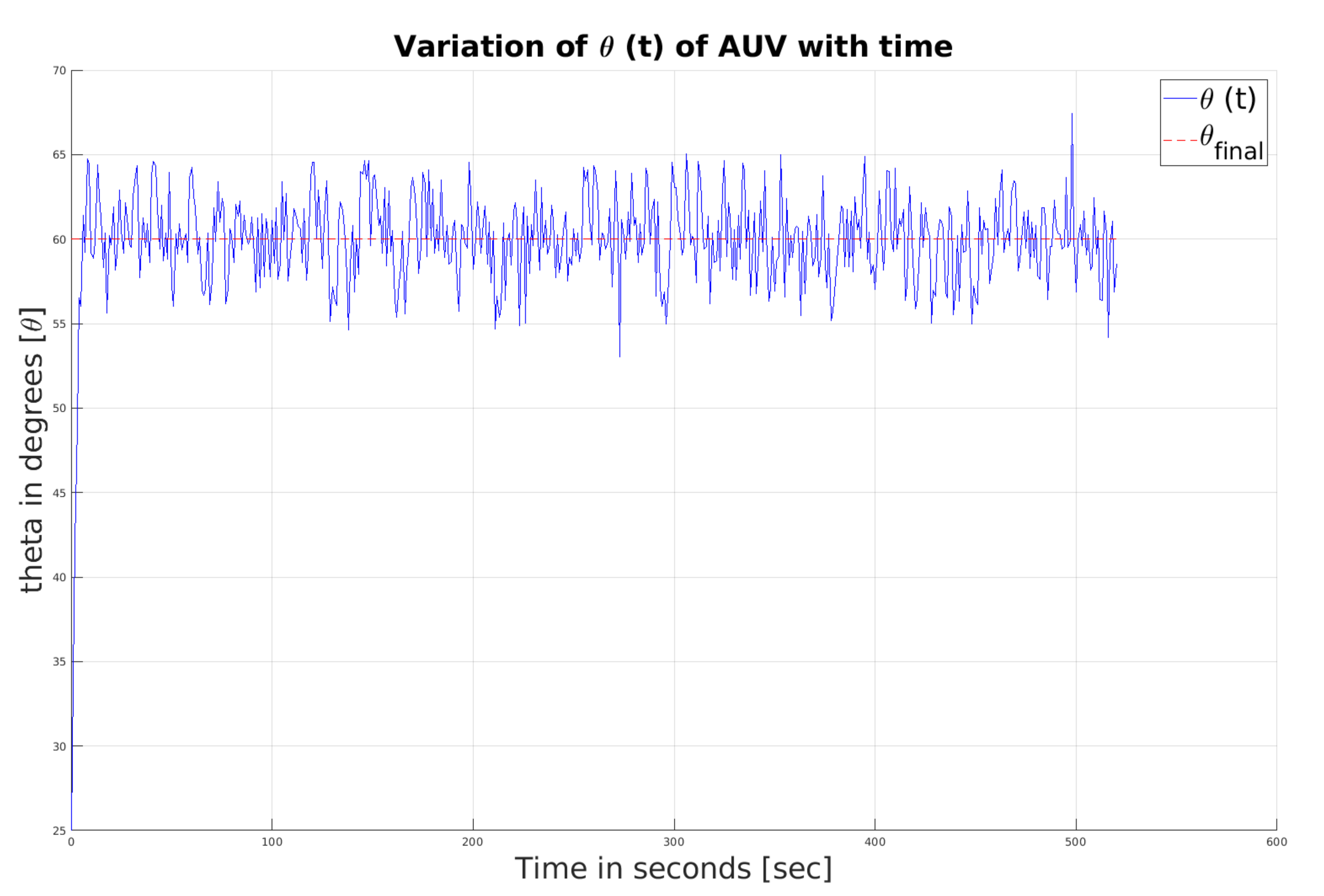
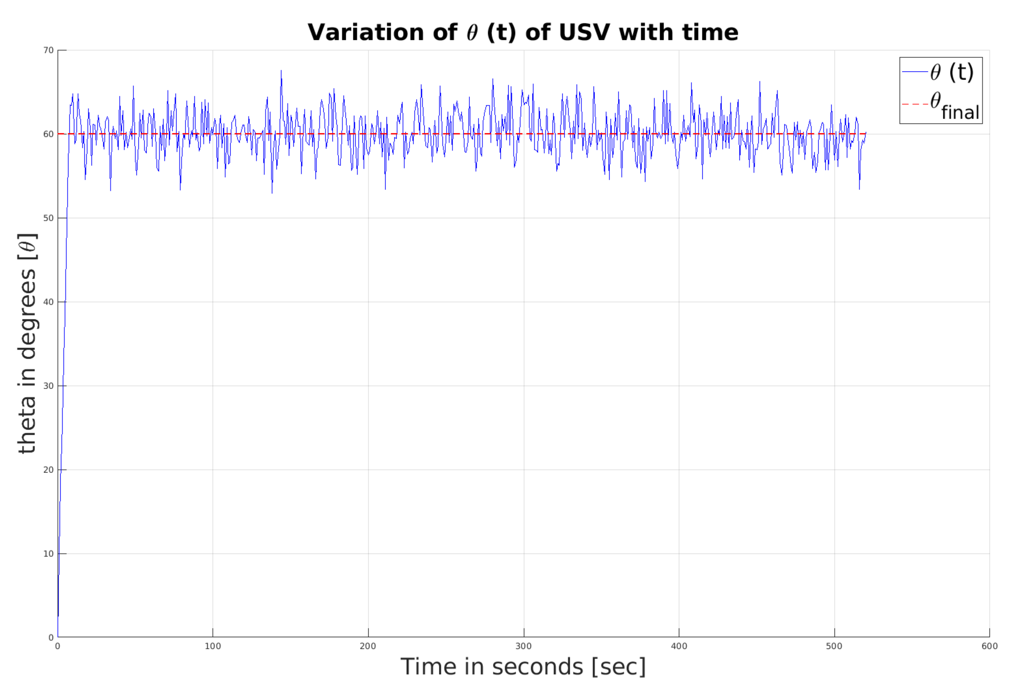
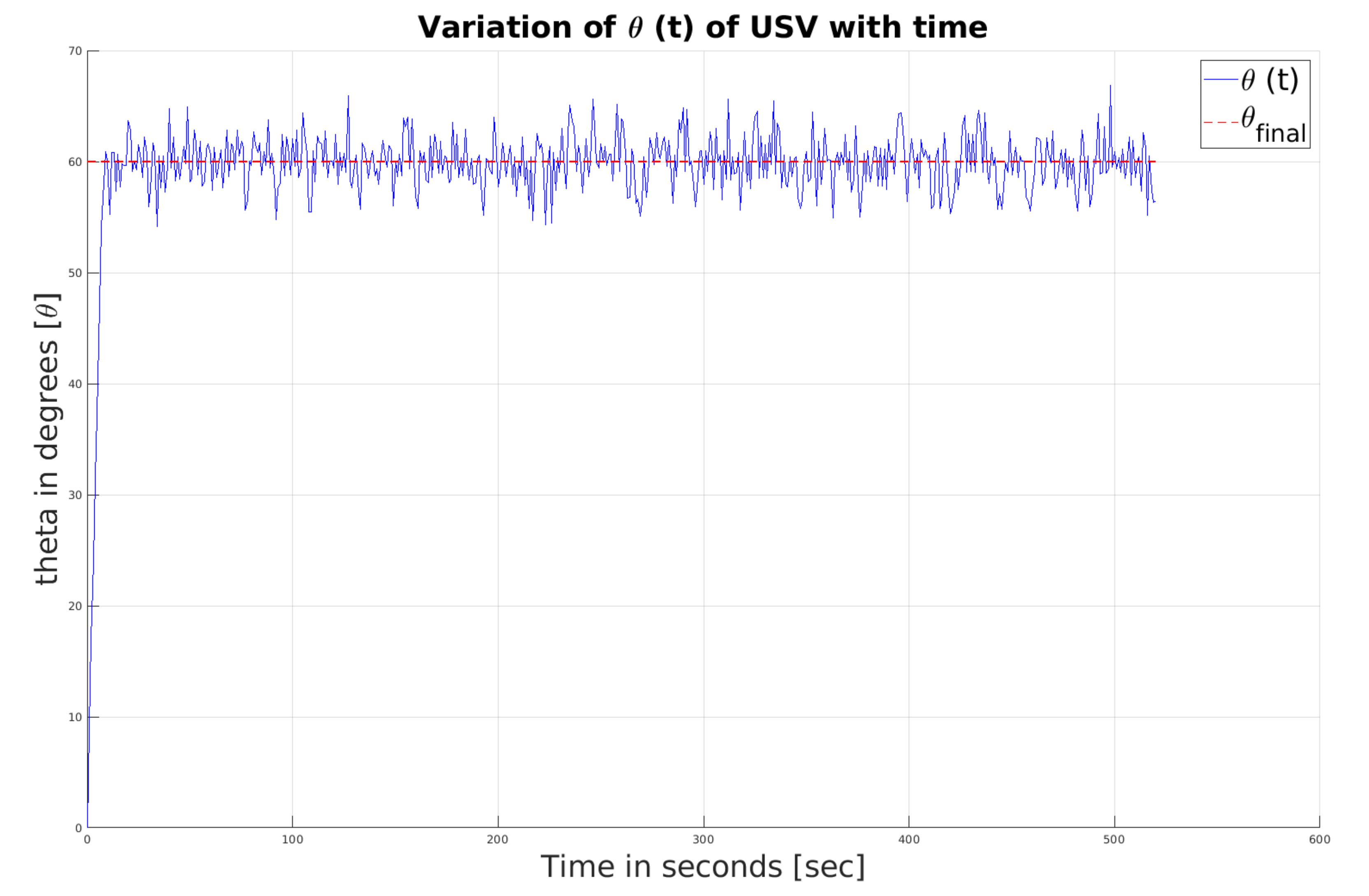
to the AUV at time t = 0. Once the AUV obtains information, both vehicles travel in the same direction. Within 20 s, both of them achieve the same heading angle; see
Figure 1 and
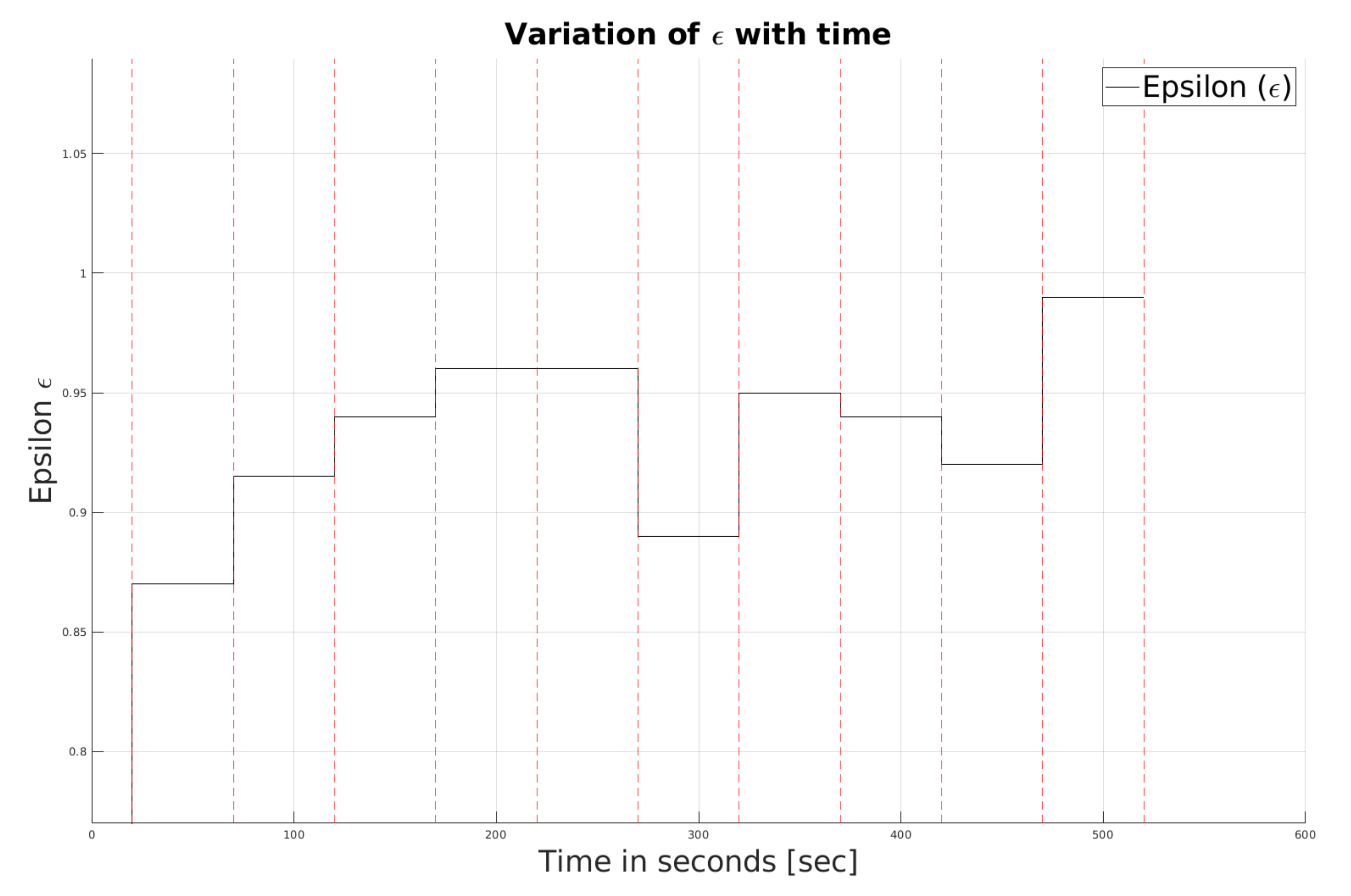
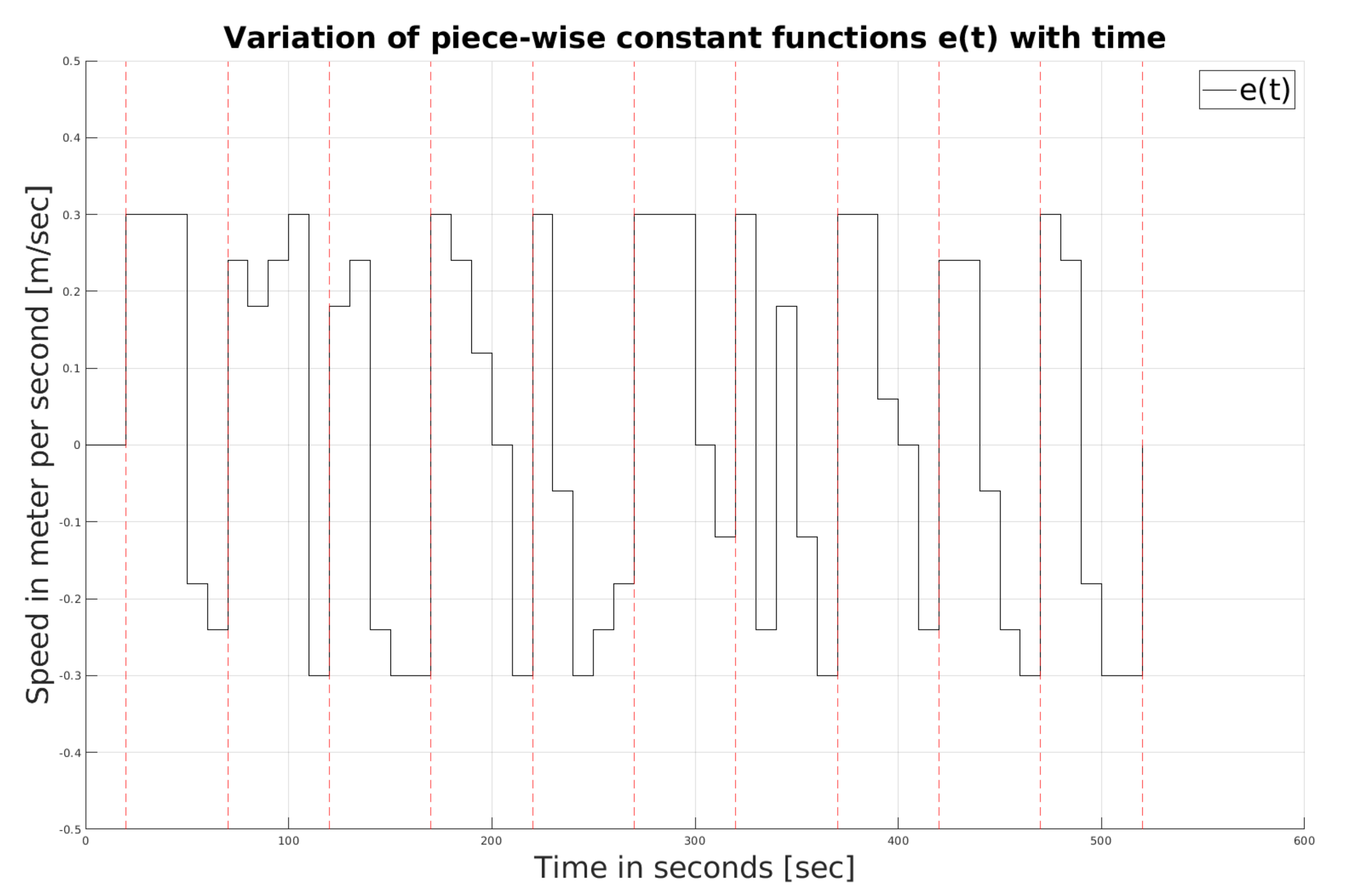
Figure 2. The chattering visible in the figures is due to the presence of a sign function in the controller. At the end of 20 s, Assumption III.1 is verified; subsequently, the value of the
function is generated for the next 50 s; see
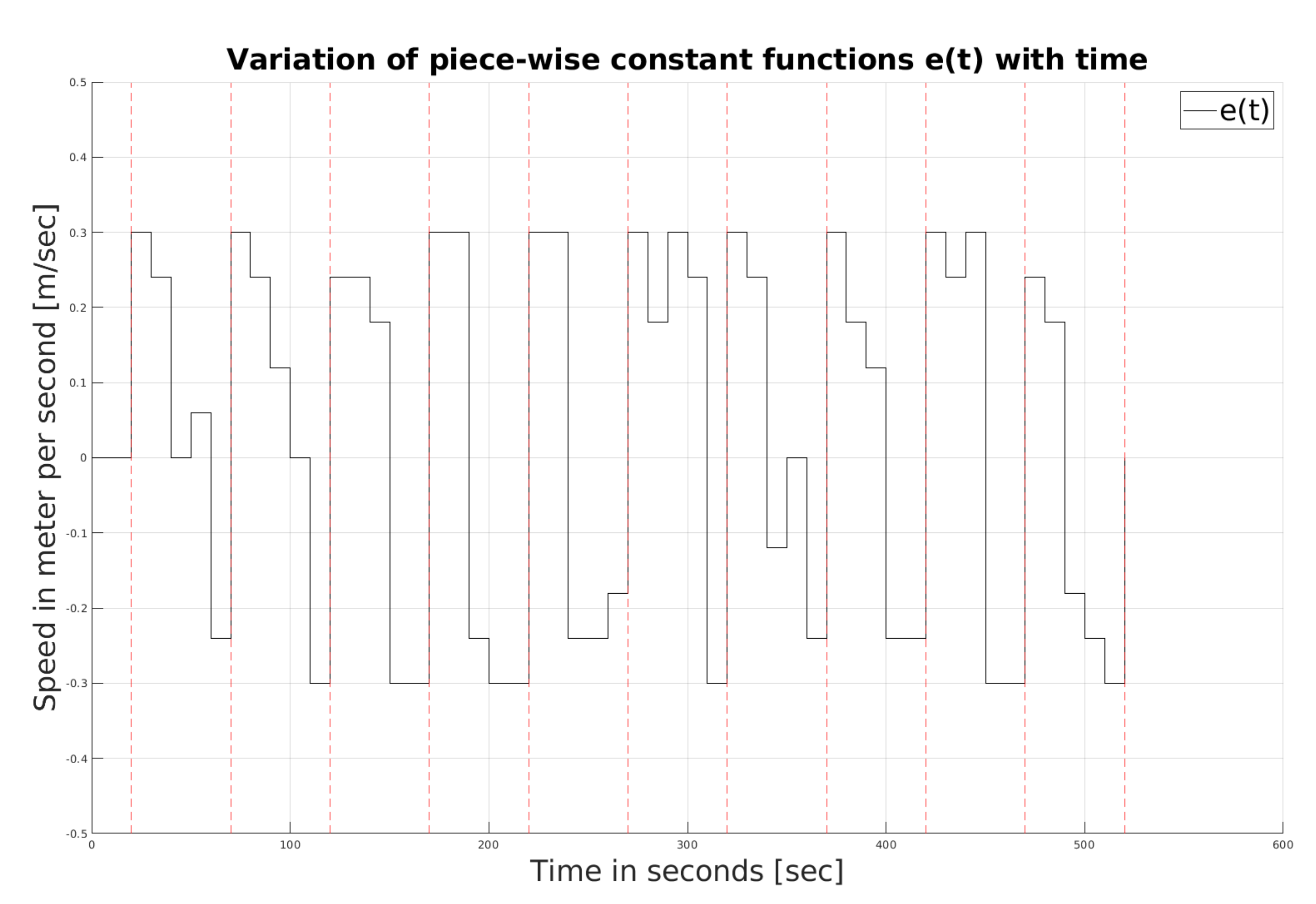
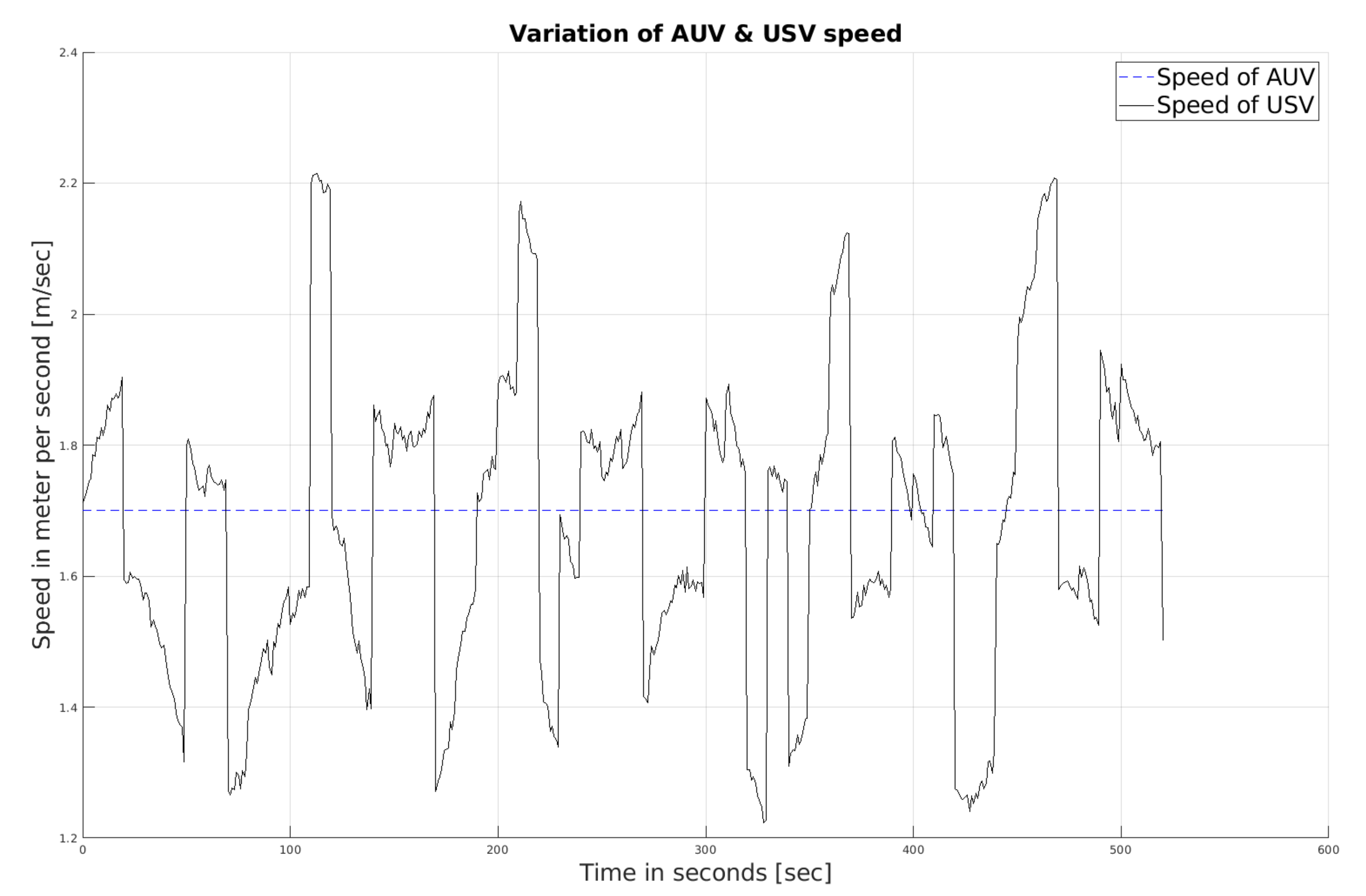
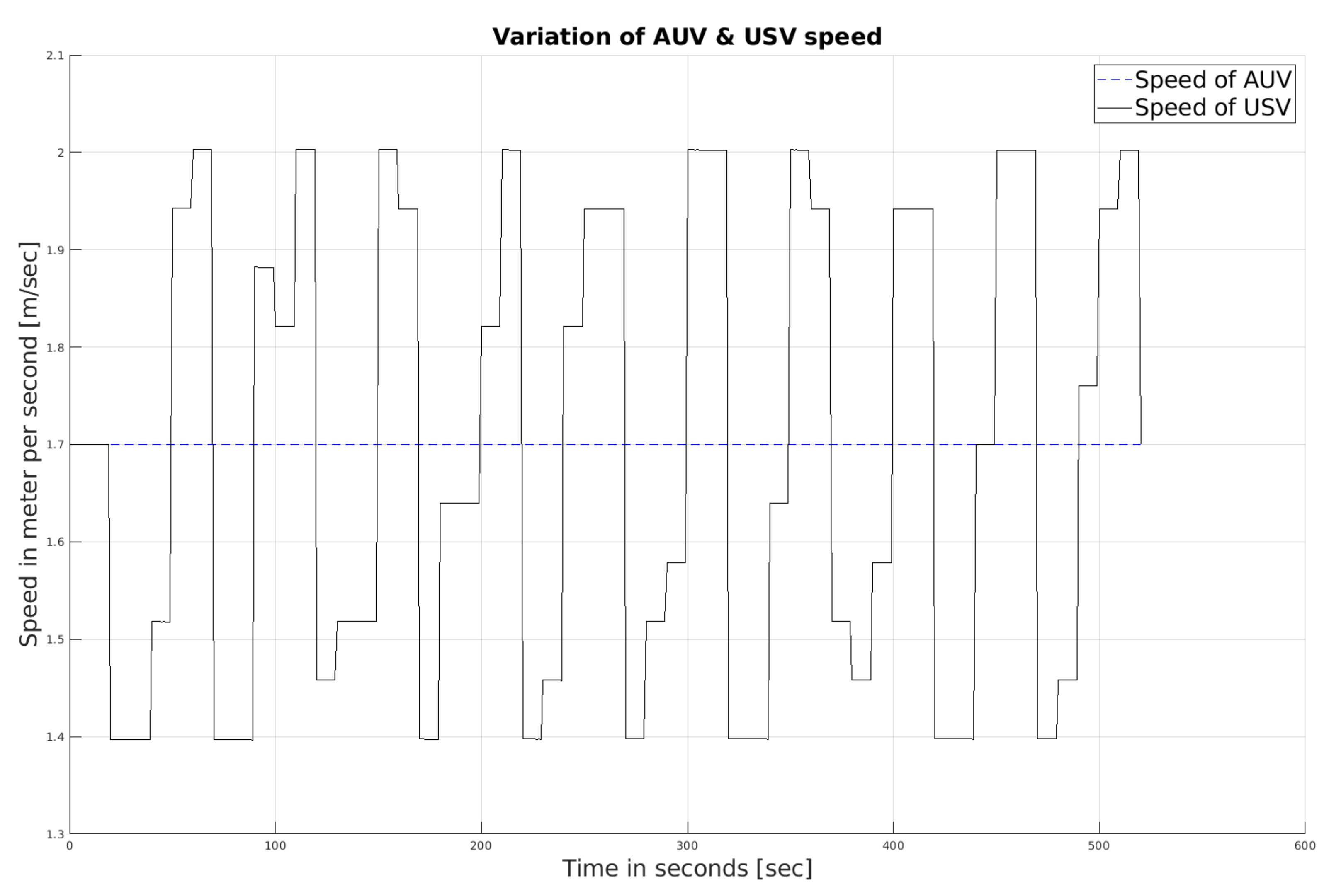
Figure 3. Once calculated, the navigation law NL2 applies to the USV, controlling the speed of the USV; see
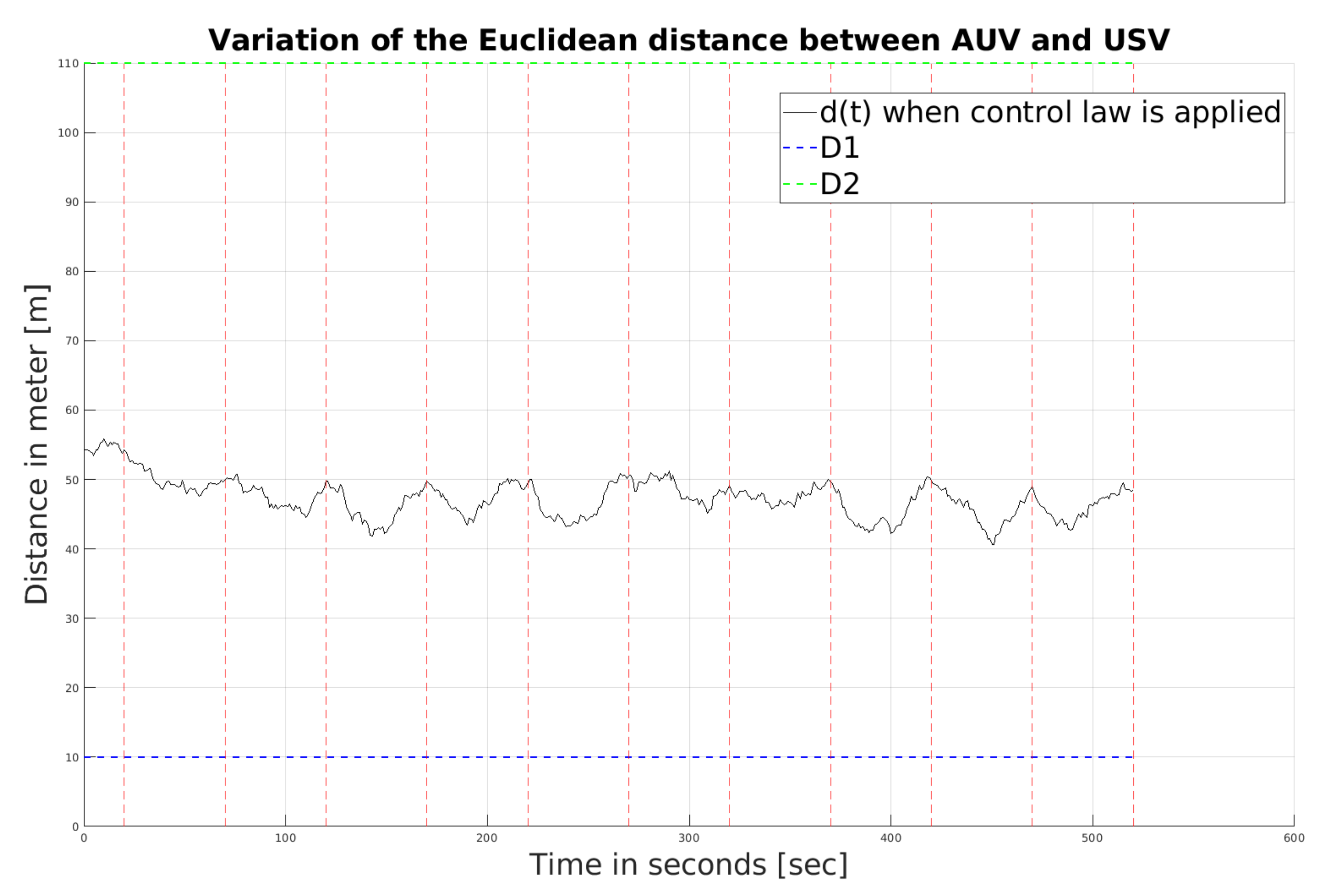
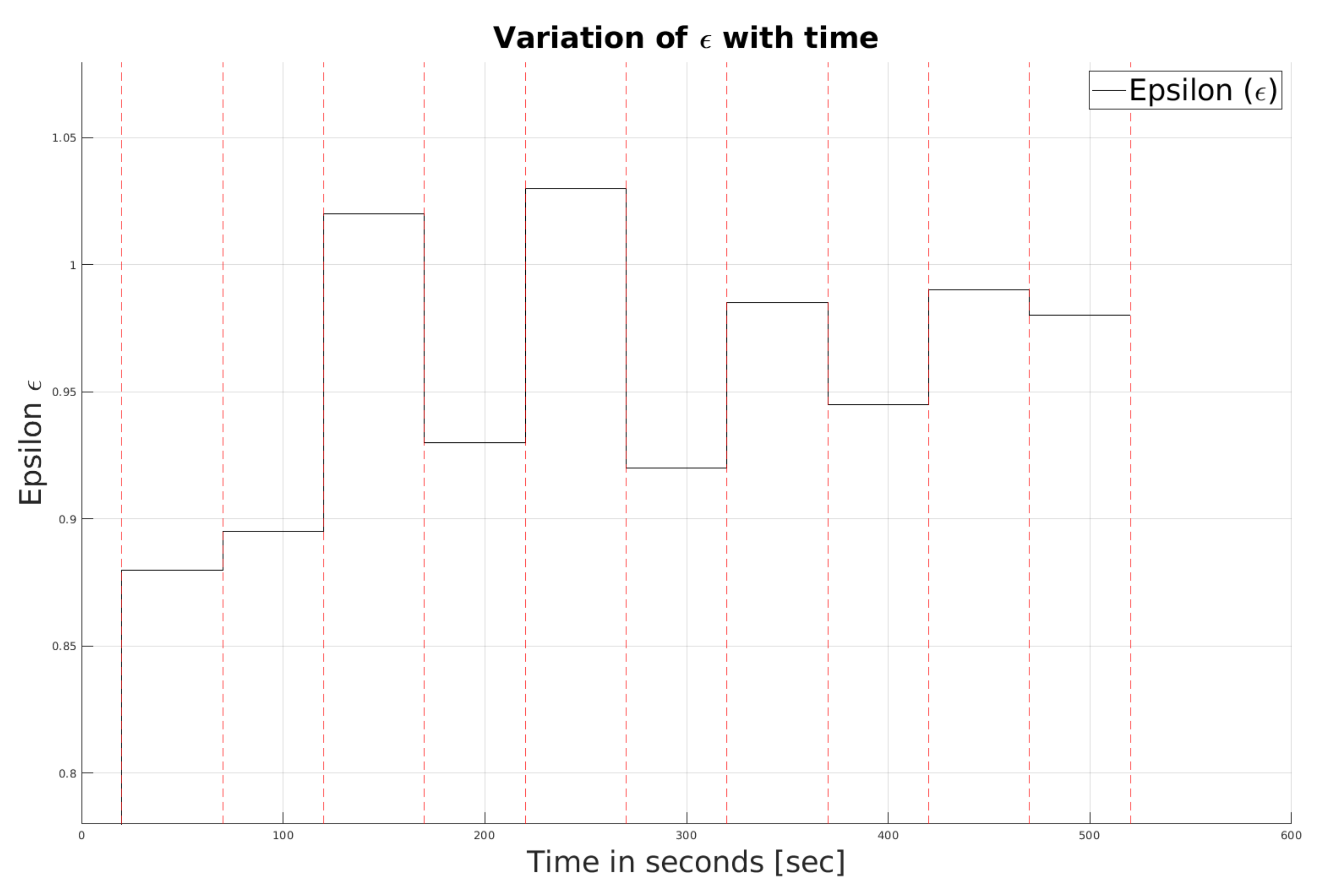
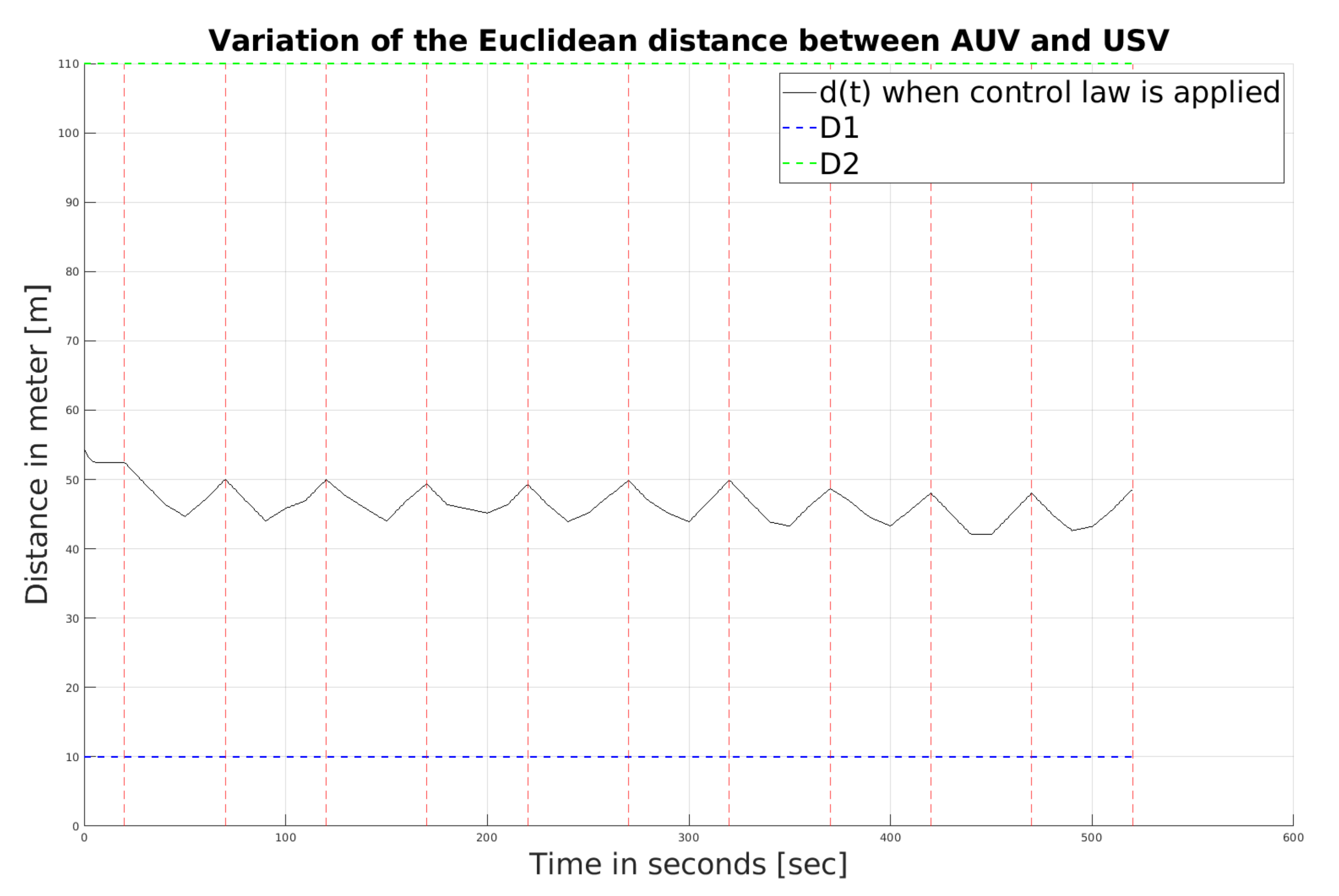
Figure 4. It also causes the value of
to fluctuate as shown in
Figure 5. In a nutshell, at the end of each interval,
is calculated to compute
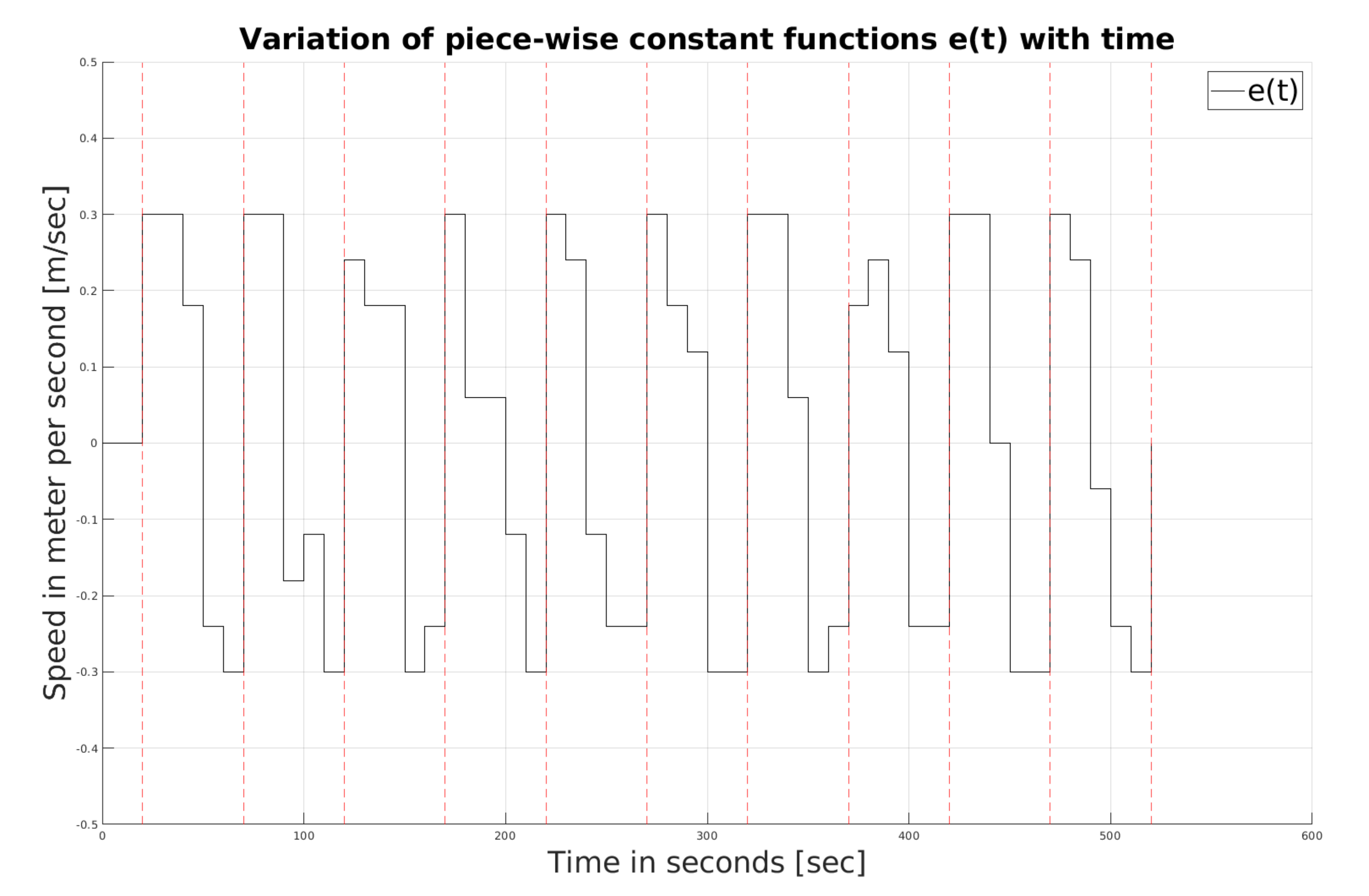
for the next interval. The whole process is repeated until the end of the simulation. In each interval, the piecewise constant
has to be selected carefully before calculating
; see
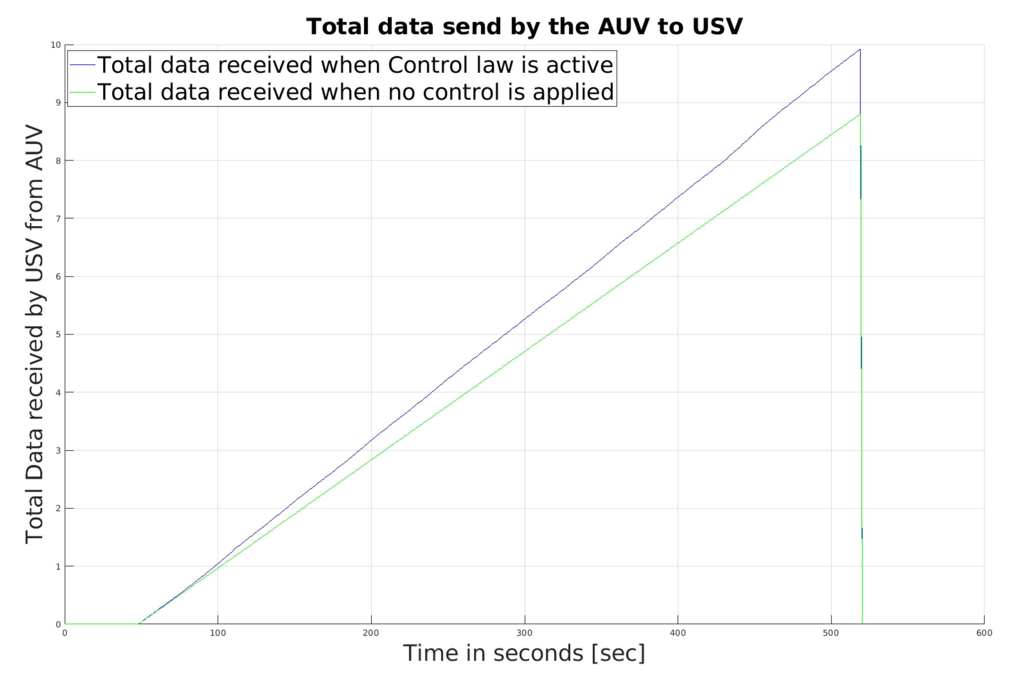
Figure 6. In general, the distance is increased to avoid collision and decreased to improve data transmission. As observed from
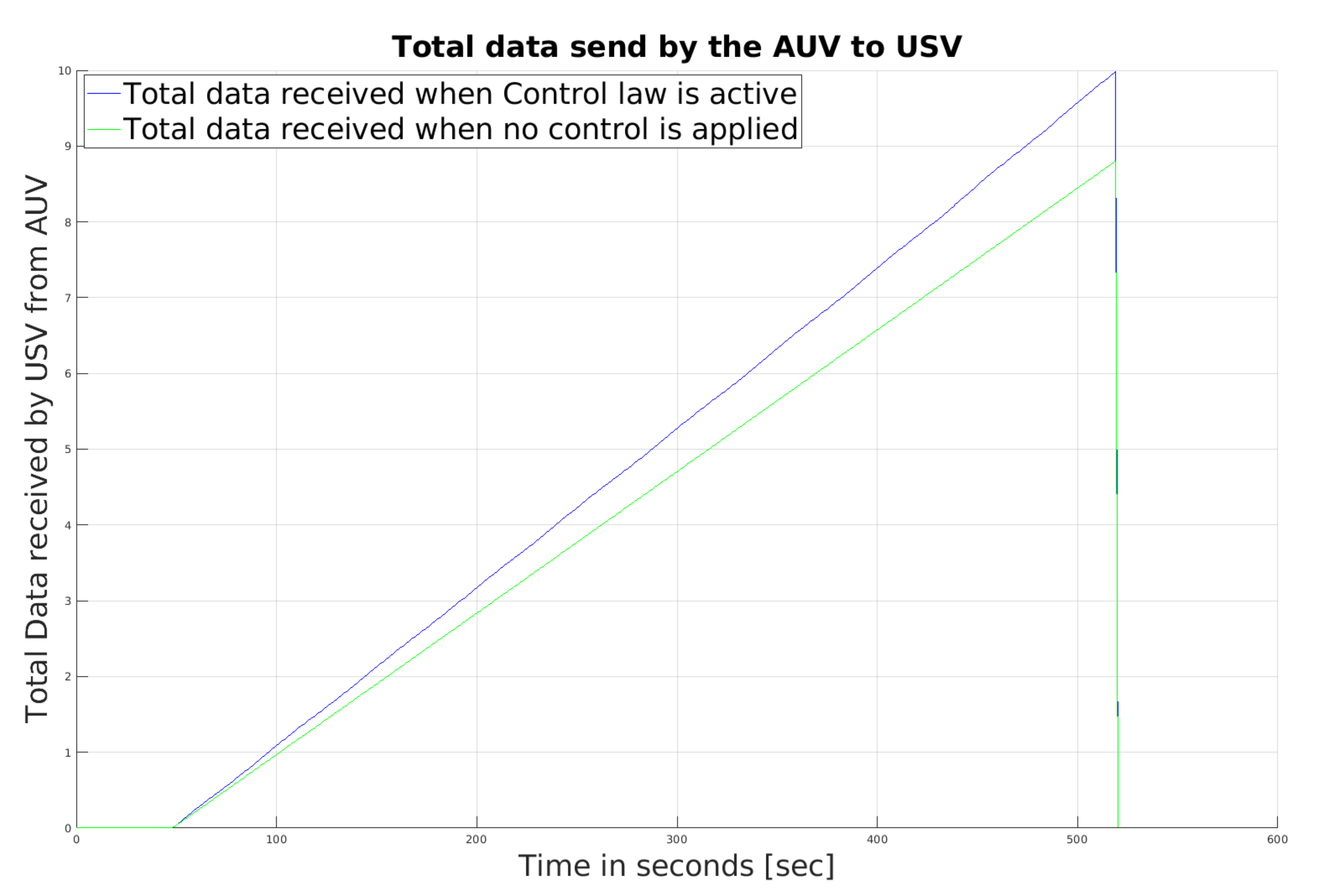
Figure 5, over ten intervals, the separation between the AUV and the USV decreases, and the probability of collision increases slightly. The total amount of data sent from AUV to USV until time
t, where
, is illustrated in
Figure 7. As seen from the figure, when NL1 and NL2 are active, the cumulative number of data packets received by USV at time
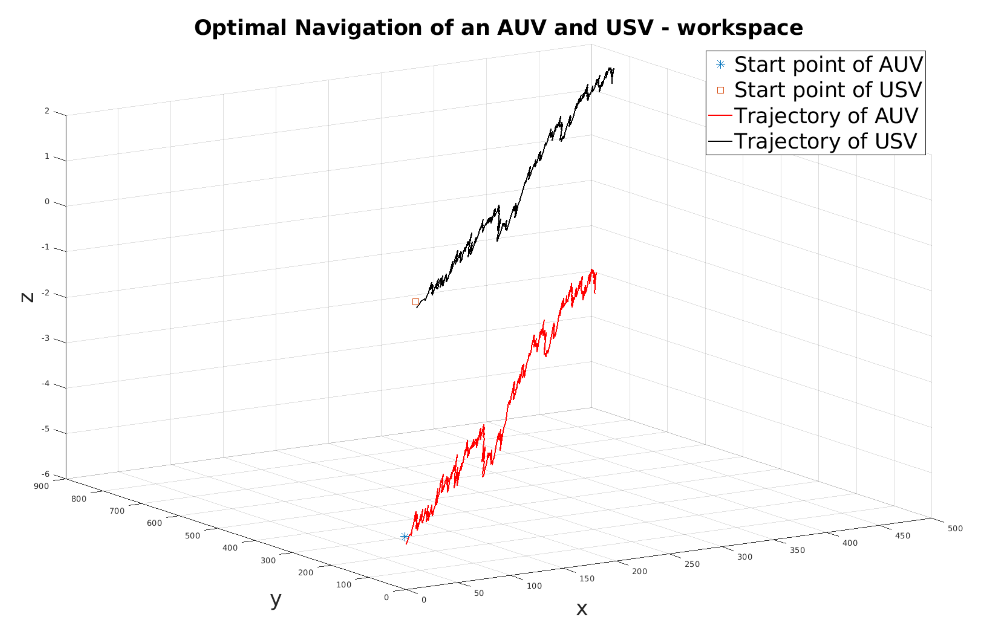
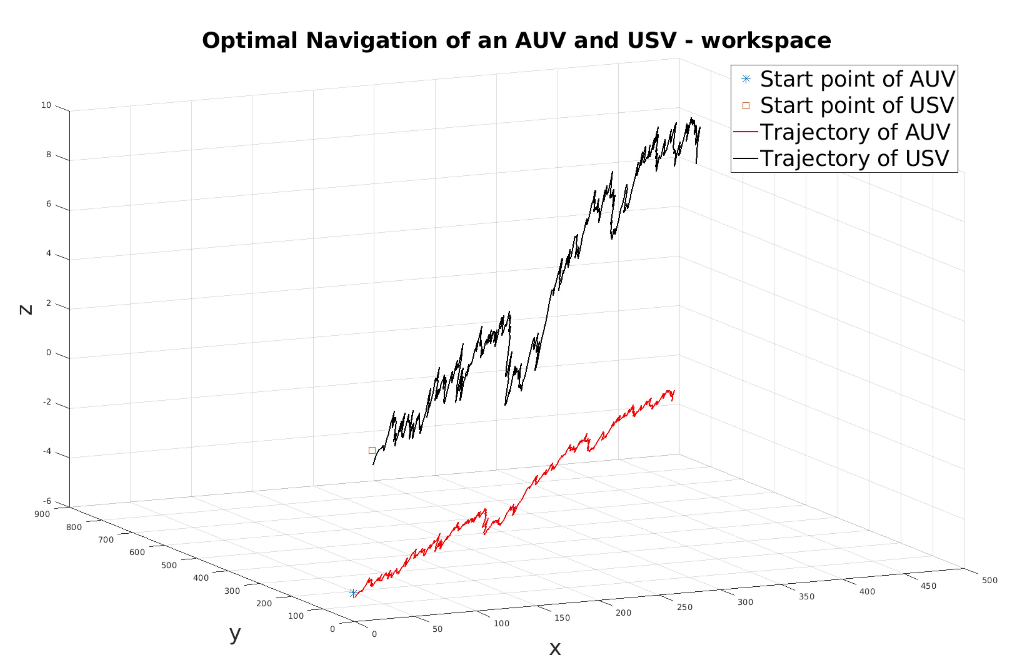
t is greater than when only NL1 is active. The trajectory of both vehicles looks straight after the first 20 s. The AUV follows the USV as shown in
Figure 8.
5.2. Scenario II
White noise is added to the motion models of the USV and the AUV. A normally distributed random signal
and
with zero mean is added to the motion model of the AUV and the USV. The variance of
is
and
is
, respectively. As a result,
, the relative speed and bearing angles of the AUV and the USV, has noise components; see
Figure 9,
Figure 10,
Figure 11 and
Figure 12. Overall, the system is stable in the presence of uncertainty in the model. In comparison with the previous scenario, trajectories of variables, such as
, constant
, speed of USV and
are different. The values of
are distinct at each time interval. The
function depends on
while the other parameters are constant. Therefore, the noisy model leads to different
from Scenario I after the initial 20 s. Dissimilar
functions are computed for subsequent intervals. Hence, by the end, completely different trajectories of
,
,
and the speed of the USV are observed in
Figure 9,
Figure 10,
Figure 13 and
Figure 14. The paths of the AUV and USV during the simulation time are shown in
Figure 15. The uneven motion is due to the noise. The amount of data transmitted from AUV to USV at time
t is similar to Scenario I as seen from
Figure 16.
5.3. Scenario III
This scenario tries to mimic real-life conditions and test the performance of the algorithm. White noise is added to the speed of the USV and the motion models of both vehicles. Like the previous case, noise signals
and
are added to the motion models. Moreover,
is added to the speed of the USV. The variance of
is
,
is
and
is
, respectively. A sinusoidal periodic function is also added to
to replicate the effect of sea surface waves on the USV. The amplitude of the wave is
ms
and its frequency is
rads
. Graphs of
and
are shown in
Figure 17. As observed, the speed of the USV varies sinusoidally. And as expected, the distance
in
Figure 18, constant
in
Figure 19 and the function
in
Figure 20 have different trajectories compared to the previous two scenarios. However, notice that in all the above scenarios, overall separation has decreased over the ten intervals. Therefore, the amount of data transfer is overall similar to previous scenarios; see
Figure 21. The variation of the bearing angles of the AUV and the USV is similar to the previous case. See
Figure 22 and
Figure 23. The path followed by both vehicles during the complete simulation shown in
Figure 24 is similar to
Figure 15.
6. Conclusions and Future Work
A novel navigation problem for two collaborating marine unmanned vehicles was introduced. In this problem, a submerged autonomous underwater vehicle acoustically transmits collected data to an unmanned surface vehicle. The aim is to navigate two autonomous vehicles so that the amount of data successfully transmitted between them using underwater acoustic communications is maximised while collisions between the vehicles are avoided. We proposed an easily implementable, real-time navigation algorithm belonging to the class of sliding mode control laws. Moreover, the developed autonomous navigation algorithm is asymptotically optimal in the sense that as the interval subdivision parameters of the algorithm tend to infinity, the value of the cost function describing the amount of successfully transmitted data converges to the global maximum. Illustrative examples and computer simulations showed the efficiency of the proposed approach.
There is considerable scope to improve the results from this preliminary investigation, particularly in regards to improved models for the system dynamics and the underwater communication systems. The models (
1) and (
3) studied in this paper are well-known kinematic models. An important direction for future research is to study more advanced models, taking into account the vehicles’ dynamics, hydrodynamic effects and underwater acoustic communications characteristics. Then the navigation laws developed in this paper will be supplemented with robust controllers such as
controllers (see, e.g., [
43] and references therein) that will stabilise vehicle motion and reduce fluctuations in vehicle headings. Moreover, the next stage of research will involve implementation and testing the developed control algorithms with real marine vehicles in a real environment. We hope to pursue these directions in future work.
In this paper, we have considered the case of a USV operating in proximity to a submerged AUV. A more challenging scenario is the case of a USV operating in proximity to a surfaced AUV. Under this scenario, the AUV has restricted or zero capability to manouevre. It is also subject to wave motions and surface currents that may cause it to sporadically submerge, at which times radio-frequency communications such as Wi-Fi will be lost, while acoustic connectivity will be particularly unreliable. This is an important and interesting direction for future research.
Finally, a challenging direction of future research is to extend the studied problem to scenarios with a USV collaborating with a few AUVs and even further to teams consisting of several USVs and AUVs. In such scenarios, we will need to develop some sophisticated decentralised scheduling algorithms that decide how each AUV selects a suitable USV and a time period for acoustic communication. Some existing algorithms for large teams of cooperating UAVs (see [
12] and references therein) might be modified for this class of problems.


