Article

Demystifying the Differences between Structure-from-MotionSoftware Packages for Pre-Processing Drone Data

1
College of Science and Engineering, James Cook University Townsville, Bebegu Yumba Campus, 1 James Cook Drive, Douglas, QLD 4811, Australia
2
GeoNadir, Trinity Beach, QLD 4879, Australia
3
TropWATER/College of Science and Engineering, James Cook University Cairns, Nguma-bada Campus, 14-88 McGregor Road, Smithfield, QLD 4878, Australia
*
Authors to whom correspondence should be addressed.
Drones 2022, 6(1), 24; https://doi.org/10.3390/drones6010024
Submission received: 16 December 2021 / Revised: 9 January 2022 / Accepted: 9 January 2022 / Published: 14 January 2022
(This article belongs to the Special Issue Feature Papers of Drones)

Abstract

:
With the increased availability of low-cost, off-the-shelf drone platforms, drone data become easy to capture and are now a key component of environmental assessments and monitoring. Once the data are collected, there are many structure-from-motion (SfM) photogrammetry software options available to pre-process the data into digital elevation models (DEMs) and orthomosaics for further environmental analysis. However, not all software packages are created equal, nor are their outputs. Here, we evaluated the workflows and output products of four desktop SfM packages (AgiSoft Metashape, Correlator3D, Pix4Dmapper, WebODM), across five input datasets representing various ecosystems. We considered the processing times, output file characteristics, colour representation of orthomosaics, geographic shift, visual artefacts, and digital surface model (DSM) elevation values. No single software package was determined the “winner” across all metrics, but we hope our results help others demystify the differences between the options, allowing users to make an informed decision about which software and parameters to select for their specific application. Our comparisons highlight some of the challenges that may arise when comparing datasets that have been processed using different parameters and different software packages, thus demonstrating a need to provide metadata associated with processing workflows.

1. Introduction

Drone data use within environmental sciences has increased considerably over the past 20 y. This is due in part to the increased availability of drone platforms on the market, technological advances providing better sensors, a longer battery life, easier-to-use systems, and enhanced structure-from-motion (SfM) software that is able to process these datasets into orthomosaics and digital elevation models (DEMs) [1]. Further, in contrast to traditional aerial survey and satellite data capture, drones are able to survey at a fine resolution from a low altitude, be deployed on flexible time schedules, and fly below clouds for unobstructed data collection [2]. In some ways, a drone can capture data more akin to field surveys, though over larger and potentially inaccessible areas, thus effectively bridging the gap between satellite and on-ground data collection across terrestrial and marine environments [3].
Drone data have been captured to provide information across a range of environmental fields, predominantly to assess vegetation coverage, composition, and/or structure in the terrestrial environment (e.g., [4,5,6,7,8]). However, they have also been used to study a range of other environments, including mangroves [9,10,11], oyster reefs [12], coral reefs [13,14], coastal dunes [15,16], and seagrass beds [17]. They have also been used to identify invasive plant species [18,19,20] and estimate animal populations [21,22,23]. Drones are also commonly used within agriculture (e.g., [24,25]), forestry [26], and urban settings (e.g., [27,28]).
Most of these environmental applications require the drone data to undergo some form of preprocessing before the data are suitable for mapping analyses. Typically, individual drone images will retain metadata not only of the time and date of capture, but also the x, y, z coordinate location of the drone (longitude, latitude, altitude), its orientation, and the angular rotations of the platform and camera. The combination of imagery and metadata is used by SfM photogrammetry software to commence the pre-processing workflow.
The two most commonly used outputs of an SfM workflow include a DEM and an orthomosaic. DEMs are spatial datasets that describe surface terrain features and are broken up into two categories: digital terrain models (DTMs) and digital surface models (DSMs) [29]. DTMs measure the elevation of the mapped surface, minus objects on the surface (e.g., trees, buildings), whereas DSMs measure the mapped elevation including surface objects. The derived DEM is then used in the process of building an orthomosaic.
Orthomosaics are created by stitching together a series of individual, overlapping orthorectified aerial images to produce a single continuous image/map [30]. This process corrects for distortions in the image, introduced by factors such as camera tilt, lens distortion, and environmental conditions [31]. The end product is a uniformly scaled, georeferenced image allowing for accurate estimation of the location, size, and shape of photographed objects.
The accessibility of drones and their derived data products allow scientists, land managers, and other users to collect and manage their own spatial datasets [1]. However, many end users remain unaware of the processes that take place within the workflow of a chosen software or the potential differences in the end product as a result of processing and software choices [32]. There are both proprietary and open-source software options available for conducting SfM photogrammetry. Provided one has sufficient skills in coding, open-source toolkits can be more flexible and allow customisation of many stages in the workflow. In contrast, proprietary software often provides a streamlined workflow to facilitate photogrammetric processing. However, these packages are often referred to as a “black box”-type solution because they offer little control or insight for users on the internal workings of the software, and in many cases, there is limited opportunity for customisation [33].
The uptake of SfM methods in research and monitoring requires some understanding of the data acquisition and image processing workflow to ensure research design repeatability and comparability [34]. Decisions in the image capturing process such as camera type, image resolution, level of image overlap, use of ground control points (GCPs), time of day, tides, and weather conditions can all affect the final orthomosaic and DEM [2]. Additionally, the different SfM software use different algorithms and processing options, which can also affect the final outputs [34]. The subtle difference in outputs between software types, combined with the limited photogrammetry background knowledge of many users of the software, means it is often difficult to reproduce or confidently compare results across photogrammetry studies.
While there have been some studies that have sought to compare the outputs provided by different photogrammetry software, they appear to have exclusively been conducted in the terrestrial environment, with a focus on forests [35,36], sandpits [37], agriculture [38,39], or urban environments [38]. Only Jiang et al. [38] investigated the output of different software across different types of datasets (urban and agricultural). There appear to be no assessments of the comparative accuracy or suitability of different photogrammetry software in processing unmanned aerial vehicle (UAV) data in marine or coastal environments that evaluate both orthomosaic and DSM outputs. This is particularly problematic since most terrestrial UAV mapping uses GCPs and real-time kinematic positioning (RTK) to enhance the accuracy of mapping outputs from photogrammetry software. Previous comparative studies that have assessed the performance of SfM software have focussed on the accuracy of GCPs compared to ground truth GPS measurements under differing levels of GCPs [37]. However, in the marine environment, the placement of GCPs and the use of RTK is extremely difficult, requiring photogrammetry software to produce orthomosaics with limited or no GCPs and RTK.
Through this research, we aim to assist others in selecting an appropriate SfM software package for pre-processing drone data. In order to do this, we provide qualitative and quantitative assessments of four desktop-based SfM photogrammetry packages, assessing their output file dimensions and specifications, orthomosaics, and digital surface models using input aerial drone data across a variety of terrestrial and marine environments, both natural and built. Finally, we compare the outputs of the software packages and against satellite-derived data in the same locations. We hope that these comparisons highlight some of the challenges that may arise when comparing spatial datasets that have been processed using different parameters and different software packages, thus demonstrating the need to provide the metadata associated with a processing workflow.

2. Methods

There are a multitude of SfM photogrammetry software packages available designed to pre-process drone data and create DEMs and orthomosaics. Within this study, we focussed on a subset of these packages and selected four of those that are commonly cited and are available in the desktop processing environment, namely Pix4Dmapper [40], AgiSoft Metashape [41], Correlator3D [42], and WebODM [43].

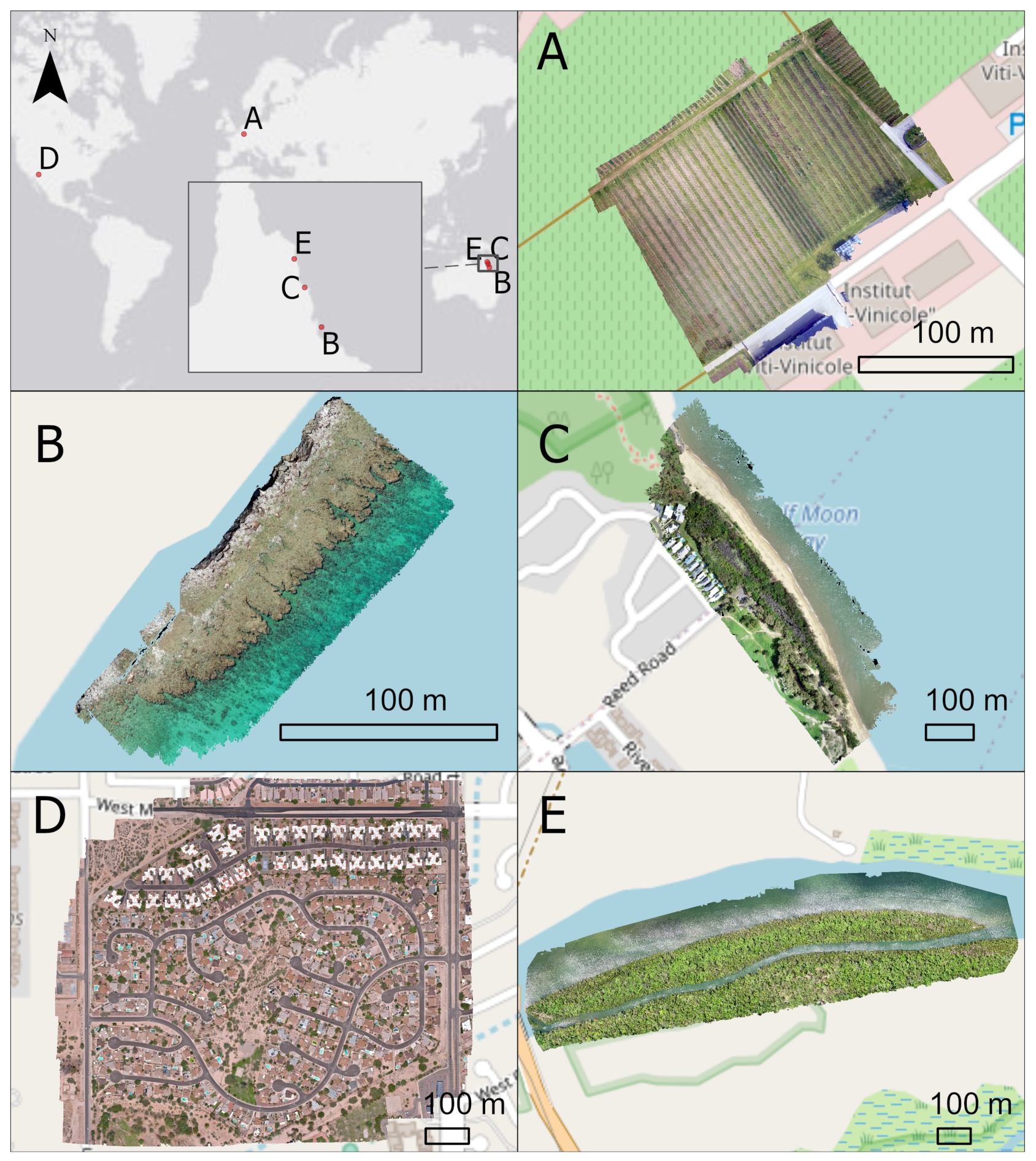
2.1. Study Sites and Input Data

Using the online drone data platform GeoNadir [44], we downloaded datasets representing variable and commonly studied ecosystems (agriculture, marine, coastal, and urban) (Figure 1). All drone images were captured during mapping missions. As such, the images have a high degree of overlap and sidelap between adjacent photos, were captured using an RGB camera at nadir angle, and include a location at the time of capture in the image metadata. The dataset specifications are included in Table 1.

2.2. Software Packages

We selected three commercial and one open-source desktop SfM photogrammetry software packages to construct a DSM and orthomosaic for each sample area:
  • AgiSoft Metashape 1.7.1 [41], formerly known as PhotoScan, is one of the most widely used commercial software packages and is frequently cited in academic literature. It supports a range of operating systems (OSs) including Linux, macOS, and Windows [45];
  • SimActive Correlator 3D Version 9.0.2 (C3D) [42] processes drone data, as well as other aerial and satellite imagery. It is only supported on Windows OS [46];
  • Pix4D Mapper (P4D) 4.2.26 [40] is available as a cloud-based solution, as well as supporting desktop OS (Windows, macOS) and mobile OSs (iOS and Android) [47];
  • Web Open Drone Map Version 2.6.4 (WebODM) [43] is a commercial-grade open-source software for drone image processing. Based on the open-source command line toolkit Open Drone Map [48], it can also be used across Linux, macOS, and Windows OS.
Figure 1. Study site locations and orthomosaic examples: (A) a vineyard (6°21 14.62042592 E, 49°32 41.87405578 N) located at Remich, Luxembourg [49]; (B) Fringing Reef on Yanooa (Pelorus) Island on the Great Barrier Reef (146°30 03.20650026 E, 18°33 37.06807973 S) located in Queensland, Australia [50]; (C) coastal suburban recreational beach (145°42 38.60723871 E, 16°47 52.90367696 S) in Trinity Park, Queensland, Australia [51]; (D) urban residential block (111°03 33.67593896 W, 32°20 56.84116378 N) located in Tucson, Arizona, USA [52]; and (E) Lung Island (145°13 49.31663938 E, 15°31 16.66610816 S) in Annan River (Yuku Baja-Muliku) National Park located in Cooktown, Queensland, Australia [53]. Service layer credits: HERE, Garmin, USGS, ESRI, ©OpenStreetMap (and) contributors, CC-BY-SA.
Drones 06 00024 g001
Each of the software packages have their own manufacturer-suggested workflows, in addition to a variety of parameters that can be manually altered depending on the user requirements. In this study, we opted to follow the suggested workflow of each package, based on the assumptions that many users are likely to opt for default settings at least initially and that the default settings have been selected by the manufacturer as producing the most consistent and hopefully optimal outcomes. It was outside the scope of this study to evaluate each and every parameter within the software themselves, and we refer interested persons to the user manuals of each software for further details.
With minor variations in terminology between software packages, each follows a similar workflow including loading data, aligning photos, bundle adjustment, creating a dense point cloud and/or mesh, creating a DSM, and building an orthomosaic. We used the “True Ortho” Correlator3D wizard workflow; the “3D Maps—Standard” Pix4D workflow; and the default template for WebODM. As AgiSoftMS does not have a templated automated workflow, we selected the manufacturer-recommended components, namely align photos, optimise alignment, build dense cloud, build DEM, and build orthomosaic. We accepted the default recommended settings for each package.
While we recognise the benefit of including independent GCPs to improve the spatial registration of the output products, we did not have access to the required reference data for this study. Further, there are many circumstances where it may not be possible to obtain sufficient GCP data (e.g., in marine environments). This study therefore evaluated the software outputs in their absence, but remains relevant as a relative comparison of the “worst-case” spatial registration between each software package.
All processing was performed using a computer with Windows 10 Enterprise OS, an Intel(R) Core(TM) i7-7700 CPU @ 3.60 GHz, 32 GB of installed RAM, and an NVIDIA Quadro P1000 GPU with 4096 MB RAM. All spatial analyses to compare the output products were conducted in ArcGIS Pro [54], and quantitative analytics were completed using Python [55].

2.3. Comparing Output File Dimensions and Specifications

After processing all datasets using the manufacturer-recommended default parameters, we compared the output details for every software and dataset combination including output file size, projected coordinate system, geographic coordinate system, x and y resolution, absolute geographical coverage, and relative coverage. The areal coverage of each orthomosaic was obtained by extracting the polygon footprint of the projected DSM and orthomosaic boundary, excluding the “no data” values.
We selected the output from AgiSoft Metashape as the baseline product to which the other datasets were compared to obtain the relative areal coverage.

2.4. Comparing Orthomosaics

To compare the output orthomosaics, we assessed the following:
a
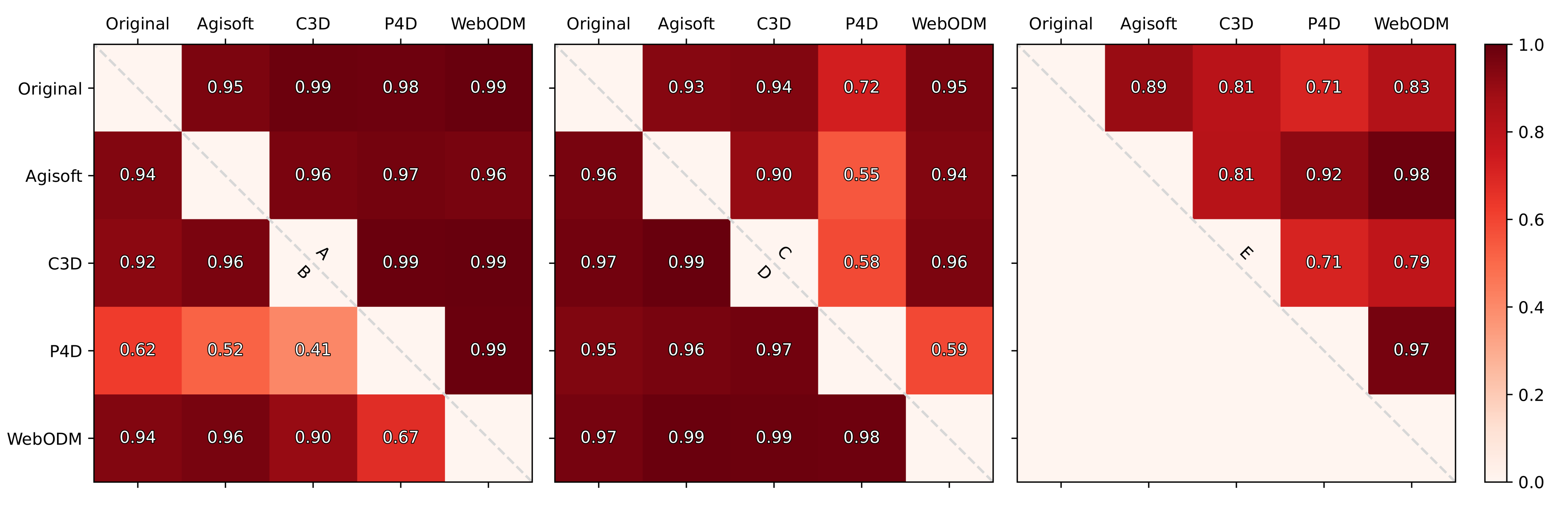
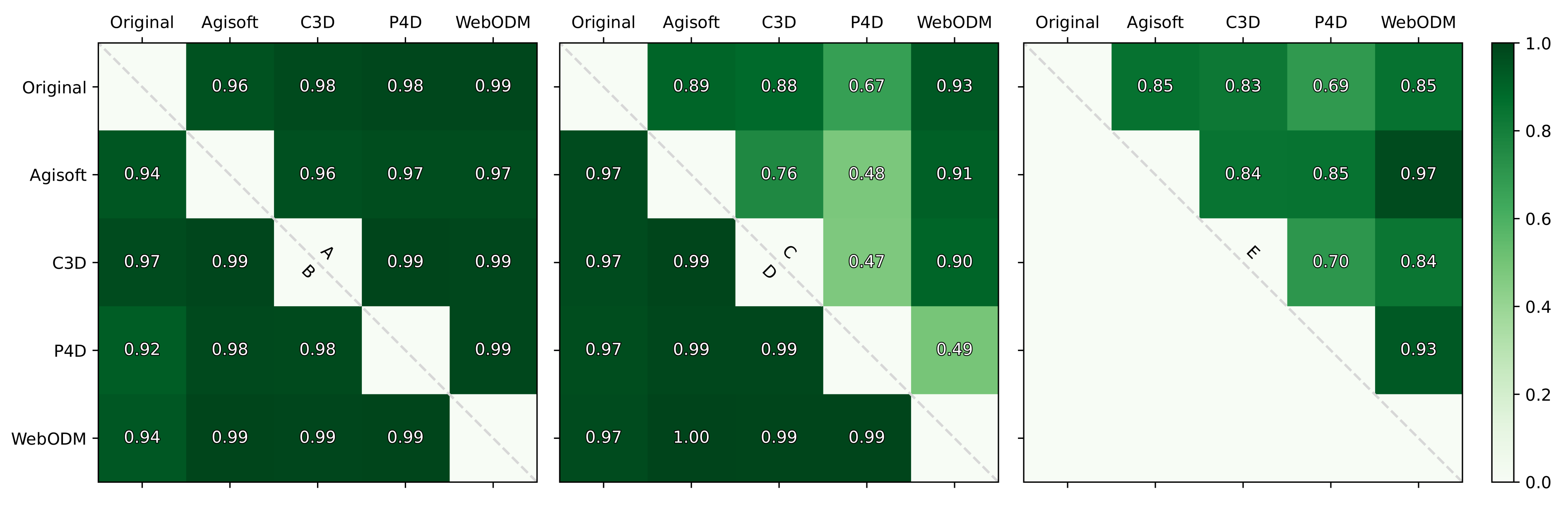
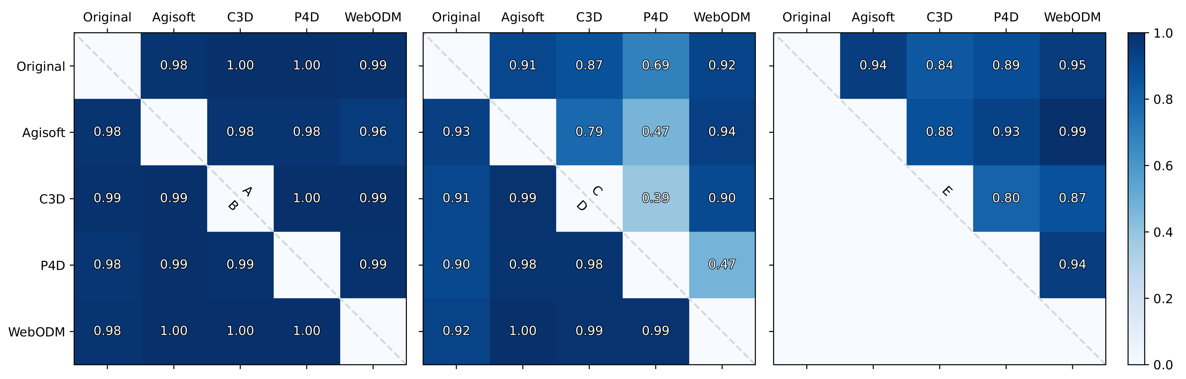
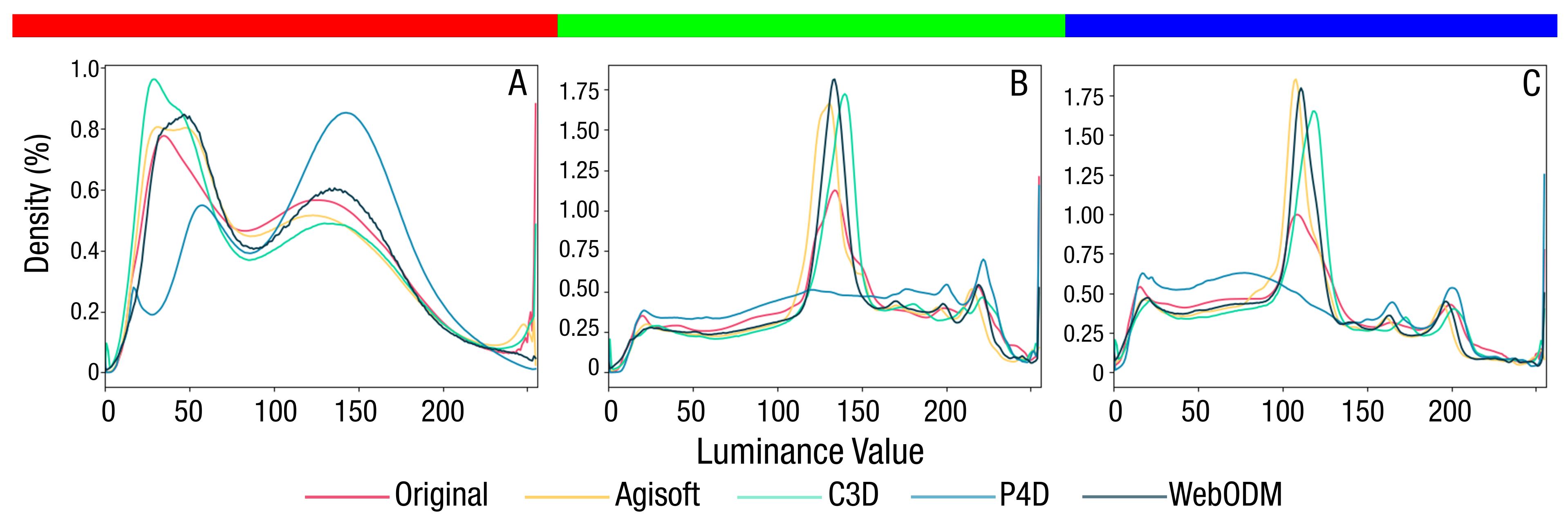
Colour correlation score: The luminance value of each pixel was extracted from each colour channel (red, green, and blue) from the original drone images, as well as the output orthomosaic. A density histogram was subsequently plotted to visualise the similarity between the unprocessed and the processed image of each colour band. A correlation score [56] was also calculated to quantify the resemblance of each histogram with each other using the equation below:
d H 1 , H 2 = l H 1 ( I ) H ¯ 1 H 2 ( I ) H ¯ 2 l H 1 ( I ) H ¯ 1 2 i H 2 ( I ) H ¯ 2 2
where H 1 and H 2 are the colour density histograms of any two out of five sources (original drone images and outputs from four software) being compared,
H ¯ k = 1 N j H k ( J )
and N is the total number of histogram bins (256 for 8 bit true colour images). A correlation score close to one indicates high similarity between the colour density of the input images and that of the orthomosaic, while a score approaching zero indicates low similarity;
b
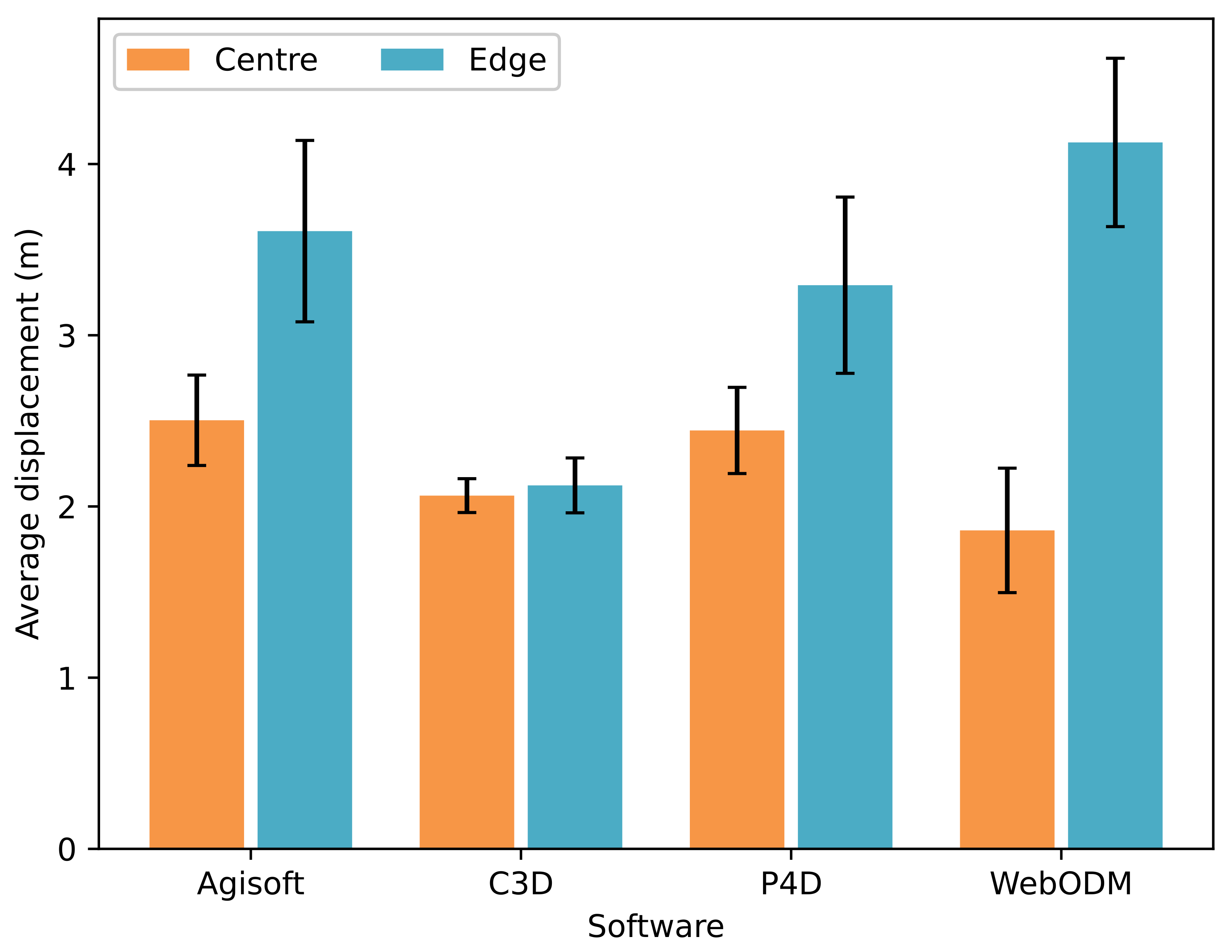
Geographic shift: As no GCPs were available, traditional horizontal and vertical accuracy assessments (i.e., [37]) could not be conducted; instead, Dataset D had very clear and identifiable features within an urban environment, and we used it to calculate the geographic shift resulting after processing with the different software packages. We digitised the polygon boundaries of 20 identifiable features across each of the four orthomosaics, plus a reference satellite image available within the Esri ArcGIS Pro base maps [57]. We ensured that 50% of identifiable features were outlined in the centre region (within 150 m of the orthomosaic centre) and 50% around the edge (within 150 m of the orthomosaic edge). We then calculated the centroid coordinates of each polygon and the distance between feature locations in each software orthomosaic in relation to the same feature location within the satellite base map. Averages (±SE) of the distance from satellite features were calculated for each software at both the centre and edge of orthomosaics;
c
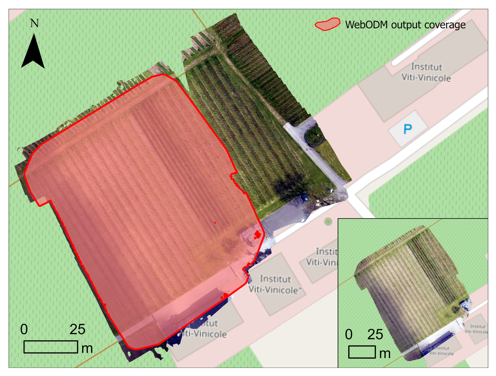
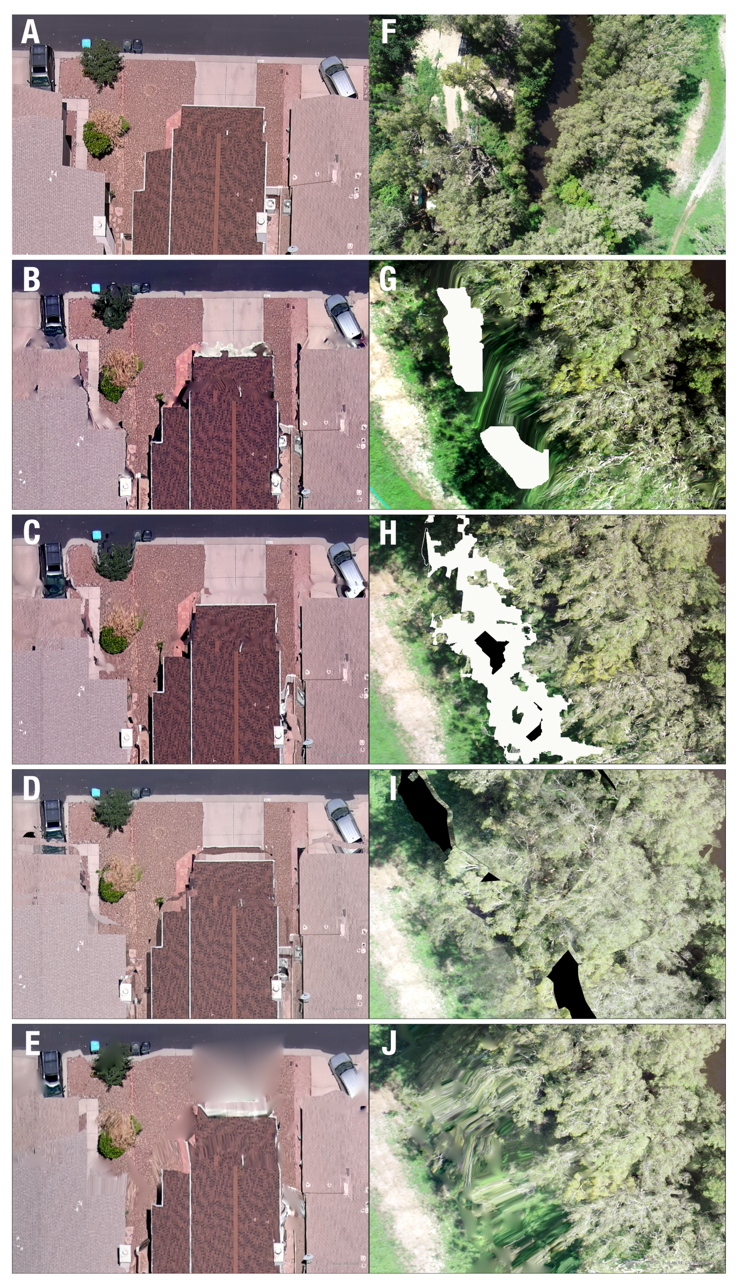
Visible artefacts: All orthomosaic outputs were visually scanned through to select obvious distortion and artefacts in the map, ensuring both the middle and edges of the datasets were evaluated.

2.5. Comparing Digital Surface Models

DSMs are often associated with various uncertainties and errors that could happen at either the data collection time or during the processing time [58]. In the absence of high-resolution LiDAR or field-verified elevation data, all DSM outputs were compared to each other and to the DSM derived from the Space Shuttle Radar Topography Mission (SRTM) DEM 1 Arc-Second Global data (approximately 30 m resolution) [59]. At each site, the four SfM-derived DSMs, in addition to the SRTM DSM, were paired up with each other (i.e., n = 10 combinations per site). Within each pair, both DSMs were resampled to the smaller pixel size of the pair and using the following statistical measures adapted from Szypuła [60]:
a
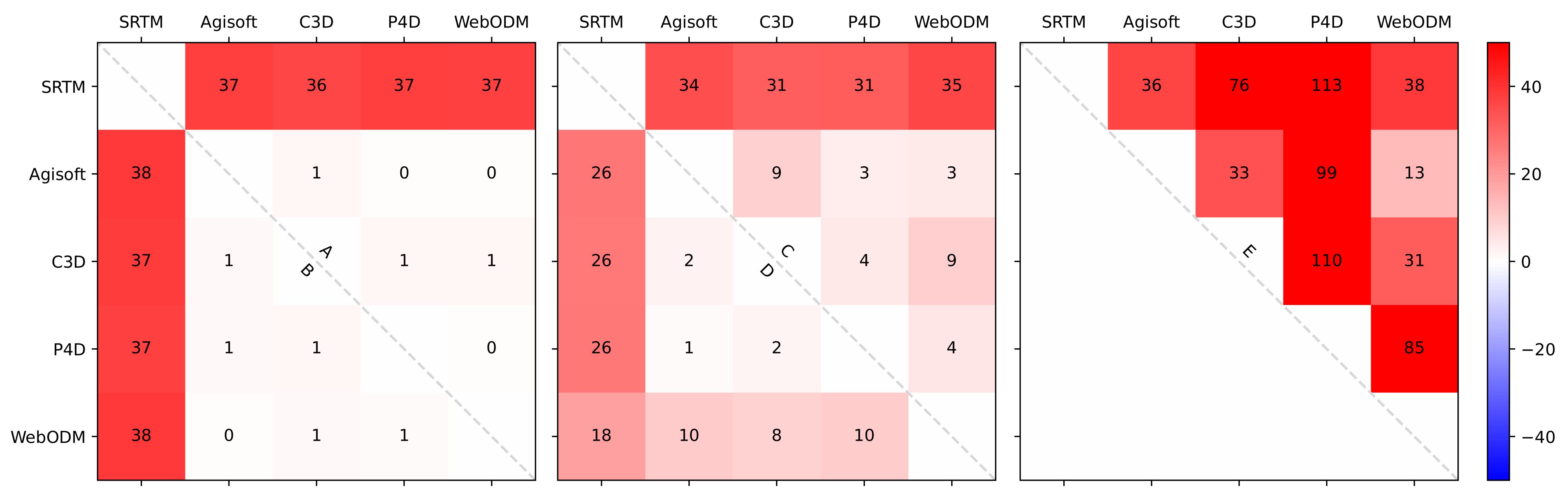
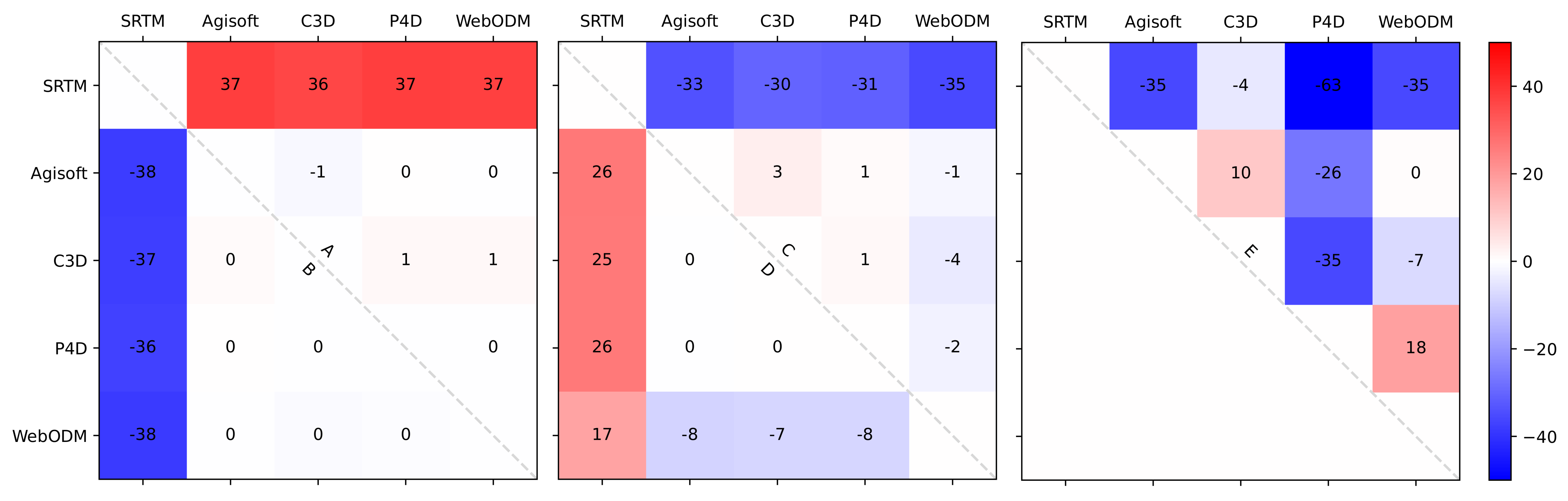
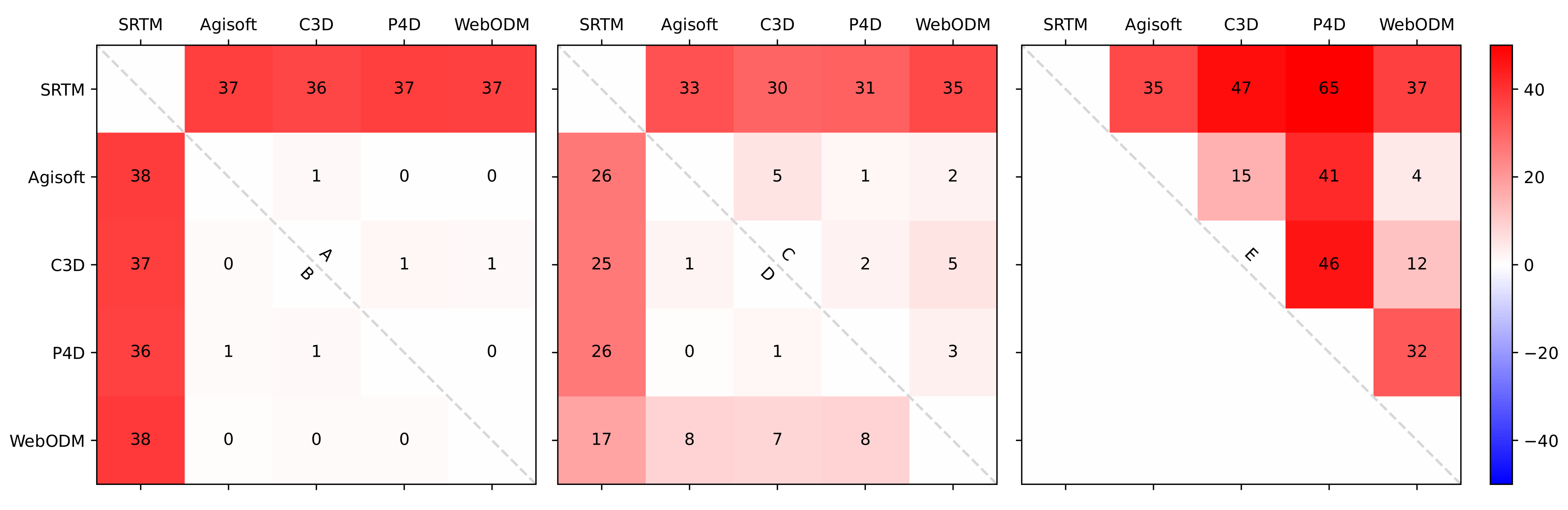
The mean bias error (MBE) measures the average magnitude of differences (i.e., errors) between any two DSM outputs. It also takes the error direction into consideration (Equation (3));
b
The mean absolute error (MAE) measures the average of the absolute differences between two DSM layers, where all individual differences have equal weight (Equation (4));
c
The root-mean-squared error (RMSE) is a quadratic scoring rule that also measures the average magnitude of the error and is the square root of the average of the squared differences between two observations (Equation (5)). Combining the MBE and MAE will demonstrate the magnitude and direction (i.e., higher or lower) of the difference between any two DSM datasets. Combining the MAE and RMSE, on the other hand, will provide the variance of the difference (i.e., all pixel have a relative uniform difference or not) between two DSMs.
M B E = i = 1 N a i b i N 1
M A E = i = 1 N a i b i N 1
R M S E = i = 1 N a i b i N 1
where a i , b i are the pixel values (i.e., elevation) at the same location of the paired up DSMs and N is the total number of overlapping pixels.

3. Results and Discussion

All software packages were able to successfully build a DSM and orthomosaic using the input datasets; however, we observed differences in the output file size, projected coordinate system, geographic coordinate system, x and y resolution, geographical coverage, relative coverage, and processing time between software packages.
Unsurprisingly, the total processing time was closely and linearly related to the number of images processed (Figure 2). In most cases, C3D was the fastest-performing software package, followed by AgiSoftMS. With the three smaller datasets, P4D was the slowest-performing software; however, with the two larger datasets, WebODM became the slowest. It is likely that the slow performance of WebODM for large datasets was due to it using the CPU for processing, while the other three packages are able to access the GPU for higher performance. Of particular note, P4D had a processing time of up to 348% more than that of C3D (Figure 3). The longer processing time for Pix4D is likely related to the additional processing steps requiring the software to generate a 3D mesh and also automatically exporting the DEM and orthomosaic. These features are not included in the recommended templates for the other packages, where 3D models are not required or where the export of files occurs after the processing stage. There was only one case where Correlator 3D was outperformed on speed (Dataset C—Trinity Park), where AgiSoftMS processed these data in 29 min compared to 34 min, or 85% of the time taken for C3D (Figure 3).
When time is money, the speed of processing is likely to influence software selection, particularly when multiple large datasets are captured. Yet, this cannot be considered in isolation, as the quality of the output is most likely the primary determinant of SfM software choice. We also note that it is possible to reduce the processing time of each of these packages by modifying the standard workflows (e.g., deselect the mesh option for P4D and WebODM), with the caveat that the modification may reduce the quality of the output products, so it should be evaluated accordingly.

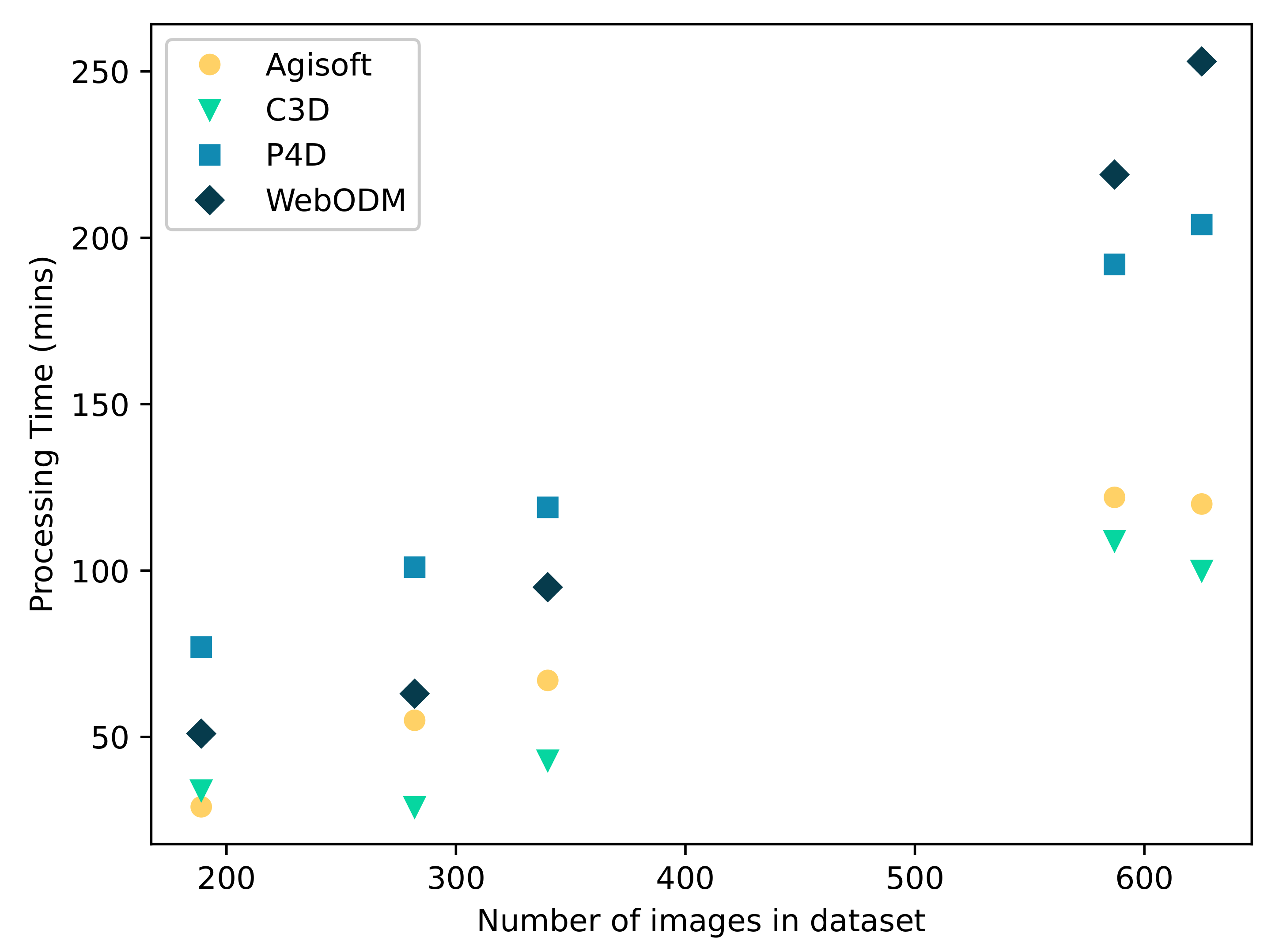
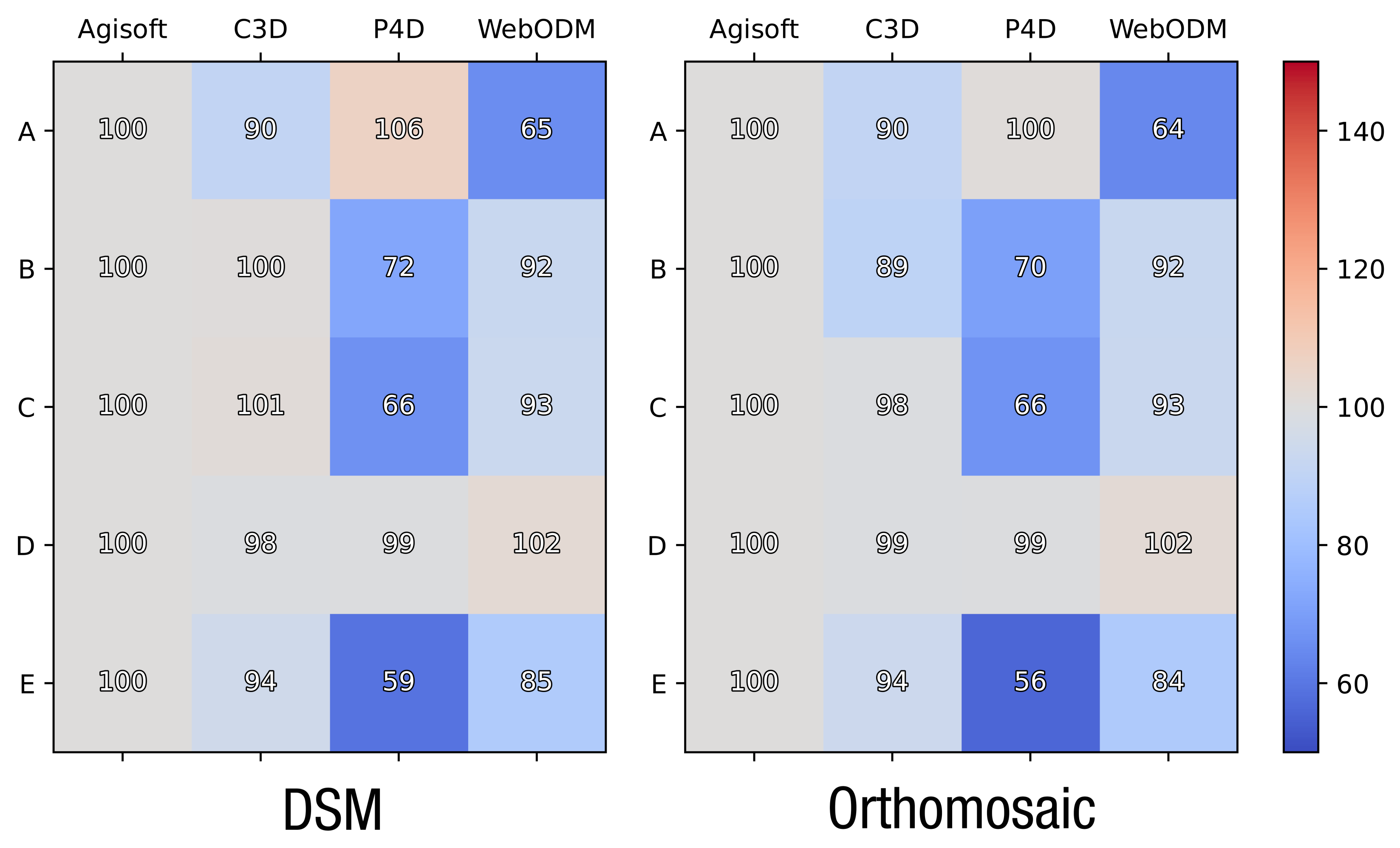
3.1. Comparing Output File Dimensions and Specifications

The output orthomosaic and DSM file sizes varied considerably between the software packages (see the details in Table A1 and Table A2). This is a result of a combination of the output image resolution and the area that was successfully processed. For example, the default WebODM processing resamples the output to a resolution of 5 × 5 cm per pixel. This lower resolution results in the lowest output file size among all software, which is useful for sharing data between collaborators or hosting on online servers. However, the loss of detail may prove problematic for some users. The other packages tend to generate the maximum resolution output by default, which is closer to the ground sample distance (GSD) of the original input drone images. As with all other parameters, the user can deviate from the default settings to stipulate the desired output resolution, and the software will resample the output accordingly. This might be important for maintaining consistency across multiple datasets, in particular for time series analysis, but resampling will inevitably alter the output image accuracy.
In combination with the output pixel size, the total areal coverage also impacts the file size. In Figure 4, we compare each of the software DSM and orthomosaic outputs to the areal coverage generated by AgiSoftMS and note the considerable differences. Pix4D in particular returns smaller areal coverages for both the DSM and orthomosaic in each of the datasets that contain water bodies (B, C, and E—Yanooa Reef, Trinity Park, and Lung Island). P4D and, to some extent, WebODM clearly have difficulty aligning and resolving water and submerged features—in particular where there is sunglint on the water’s surface—and consequently crop these features from the final products (Figure 5). WebODM failed to reconstruct the crop field on the right half of Dataset A, also resulting in a comparatively small areal coverage for those output products (Figure 6).

3.2. Comparing Orthomosaics

In comparing the orthomosaics, we aimed to evaluate the similarity in colour between the input and output data; any geographic shift between the output products and reference satellite imagery; and the visual consistency between the output product and ground features.

3.2.1. Colour Density Correlation Score

During the process of building an orthomosaic, pixel values are averaged in areas of overlap, and as we already demonstrated with the coastal datasets, some pixels are excluded entirely. The colour density correlation score provides further evidence for the differences seen between the SfM packages and original drone images (Figure 7, Figure 8 and Figure 9). In particular, the density histogram for the red channel for the P4D orthomosaics created from Dataset B (Figure 10A) are very different from the original images and other software outputs, which could be due to the cropped water feature pixels (Figure 5). The green and blue channels (Figure 10B,C) show closer alignment between all software packages with the exception of P4D, in particular in the middle range values for luminance (i.e., pixels that are neither very bright nor dark). This also results in decreased contrast across the orthomosaic scene. In cases where it is important to retain the input absolute pixel values (e.g., for quantitative mapping and assessments), it is worth further investigating the methods of feathering and averaging between images in overlapping areas to ensure the appropriate algorithms are used.

3.2.2. Geographic Shift

When compared to the satellite data available in Esri base maps within ArcGIS Pro [57], the drone data show between two and four metres of displacement (Figure 11), which is reasonable considering the positional accuracy of Global Navigation Satellite System (GNSS) units on drone platforms, in particular without additional ground control (Kalacska et al. 2020). The geographical shift is more prominent towards the edges of the orthomosaic than in the centre, due to the lower overlap of the input images in these areas. This reinforces the need to plan data capture missions that cover areas beyond the bounds of the central region of interest. In the centre of all software-generated orthomosaics, all features were within 2.50 m of the satellite features (WebODM: 1.86 ± 0.36 m, C3D: 2.06 ± 0.10 m, P4D: 2.44 ± 0.25 m, AgiSoftMS: 2.50 ± 0.26 m).
In contrast, at the orthomosaic edges, P4D, AgiSoftMS, and WebODM showed slightly larger displacement from the satellite features (Pix4DMapper: 3.29 ± 0.51 m, AgiSoftMS: 3.61 ± 0.53 m, WebODM: 4.13 ± 0.49 m). C3D, however, displayed similar displacement at the orthomosaic edges to the centre, (2.12 ± 0.16 m), making it the nearest to the satellite imagery at the orthomosaic edges. Interestingly, while WebODM appeared to be nearest to the satellite imagery in the centre of the orthomosaic, displacement at the edges was the furthest, at 2.2-times further from the satellite imagery than the centre features.
There are a range of factors in both the data collection and image processing phases that can influence geographic shift/geometrical accuracy. These include flight path, camera quality, calibration, georeferencing strategy (use of GCPs or reliance on the direct onboard georeferencing Global Navigation Satellite System (GNSS) with RTK), and the SfM algorithms [61]. While georeferencing strategies that have employed GCPs have been found to result in finer horizontal accuracy at the decimetre/centimetre scale [61,62,63], direct methods that rely on GNSS (i.e., non-RTK drones) alone have resulted in accuracies at the metre scale [31]. The metre scale of horizontal accuracy found in these previous studies that have not employed GCPs or the GNSS with RTK appear to correspond to the results of this study where average displacement ranged from 1.86–2.50 m in the centre of the orthomosaics and 2.12–4.13 m at the orthomosaic edges. If users are seeking accuracy at much finer scales, the software choice is not likely to improve the outcome greatly, and they will need to consider the addition of GCPs or the use of a GNSS with RTK to achieve centimetre-scale accuracy [64,65]. The SfM algorithms employed by each software are another possible source of variation in the geographic shift observed. Although C3D appeared more consistent in the geographic shift across the orthomosaic, this is based on the assumption that the satellite imagery represents the true location of the features. A previous study comparing both horizontal and vertical accuracy across software platforms found AgiSoft PhotoScan to be more accurate than Pix4D web-based image processing and Bundler SfM algorithms [66], but did not evaluate C3D or WebODM. Additionally, a study that compared the accuracy of five different software packages that included AgiSoft and Pix4D in their assessment found little difference in accuracy; however, this was under differing levels of GCPs as opposed to what the software can produce without these inputs [37]. While these differences were attributed to differences in the algorithms in this case, it remains difficult to directly compare the cause due to the lack of detailed information released by proprietary software developers [34,66]. This however serves as a reminder to always retain copies of the original imagery so the data can be re-processed using the best available methods, as software packages and their algorithms will change and hopefully improve over time.

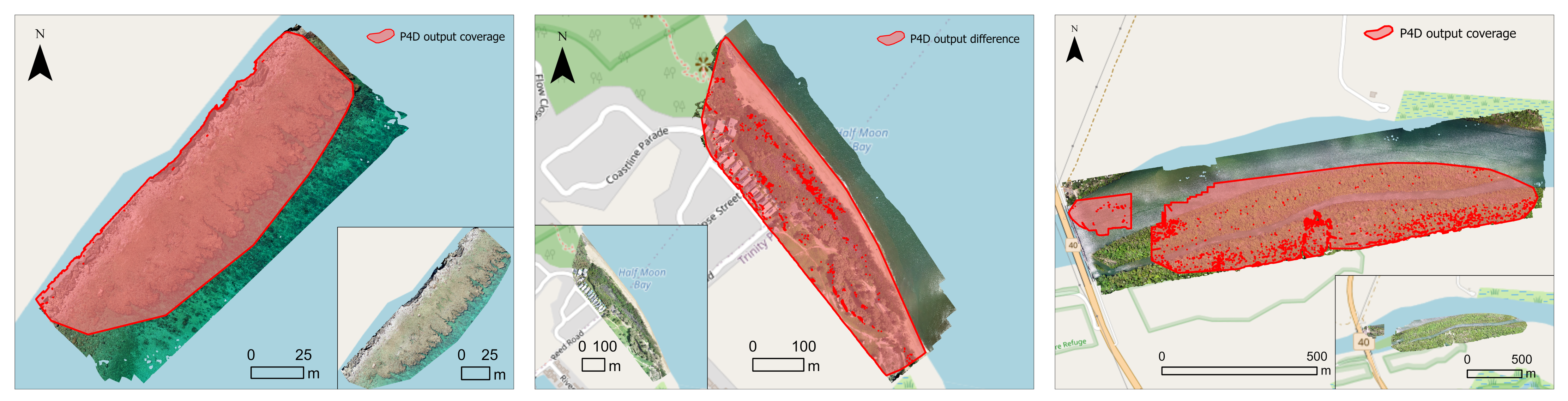
3.2.3. Visual Artefacts

The qualitative analysis of artefacts contained within orthomosaics found that all software contained more artefacts at the edges of the orthomosaic, compared to the centre. Centre artefacts were generally at a smaller scale and were only evident once viewed at increased zoom. Artefacts were also more evident in areas where DSM values in neighbouring pixels changed rapidly, such as at the edges of buildings or trees and forests (Figure 12). Artefacts presented in the form of missing data or gaps in information; “filled” data through smoothing, interpolation, extrapolation, or filtering; and cutlines at feature edges. Cutlines in the orthomosaic often produce visual artefacts at high zoom levels and will also present challenges for automated information extraction at later processing stages. Alternatively, the user can deviate from the standard workflow to create the orthomosaic using the derived DTM instead of the DSM, which tends to result in fewer visual artefacts, though can introduce a greater geographic shift of tall features in the imagery due to uncorrected radial displacement. The users must therefore determine for themselves the most suitable outcome for their specific application.
Each software’s default appears to deal with missing data in different ways. C3D simply excludes pixels where it cannot reconstruct portions of the image, presenting them as “no data” fill in the orthomosaic (see Figure 12I). Pix4DMapper and AgiSoftMS have interpolation enabled in the default settings to fill the space based on surrounding values resulting in warped or shaded sections on an orthomosaic (see Figure 12G). However, interpolation will only fill when there are enough close points, and a lack of information from close points can result in areas that are filtered out of the final DSM and orthomosaic and present as holes (See Figure 12G,H). Close inspection of the DSM and the final orthomosaic is recommended to detect holes and warped areas, as these may not be detected until zooming in on smaller features in the orthomosaic.

3.2.4. Comparing Digital Surface Model

When using similarity metrics to evaluate the output DSMs, we found that there was very little overall difference between the software outputs except Dataset E, though all differed somewhat from the SRTM data. The MAE (Figure 13) and RMSE (Figure 14) had little difference in Datasets A, B, and D, between comparison pairs, which indicates that the difference between all the pixels was fairly even. A mixture of terrestrial and aquatic features yet led to a greater variance of the difference (the RMSE of Datasets C and E was higher than the MAE). The depth (or “negative elevation”) of underwater features was inadequately represented across all models, though none of them boast a capability in this respect, and bathymetric LiDAR would certainly be a better option for deriving depth information [67].
For the datasets dominated by terrestrial features, drone-derived elevation was overestimated, producing a positive MBE in Datasets A and D when compared to the SRTM data (Figure 15). Most of the differences between the drone-derived DSMs from AgiSoftMS, C3D, and P4D were minor (seen as light shading in Figure 15), indicating that the software algorithm is not the most important factor in obtaining an accurate elevation estimate. However, WebODM displayed greater differences from the other drone-derived DSM values, in particular with Dataset D. WebODM was also more closely aligned to the SRTM data for Dataset D than the other software packages. As a previous review pointed out, the accuracies of UAV true colour image-derived DSM are comparable to those obtained by LiDAR [68]. Regardless of the usage of GCP or check points, the absolute difference between LiDAR and true colour image-derived DSM was less than 4 m [69,70]. The similarity between software outputs was as expected (Figure 13, Figure 14 and Figure 15). On the other hand, the relatively large difference between SRTM data and the software outputs is worth noting since UAV imagery is considered as a new tool to fill in the gaps between satellite imagery and in-person field surveys. However, with such a small sample size, inconsistent findings between datasets, and no GCP information, these results are inconclusive. Given the significant difference in resolution between the SRTM and the true-colour-image-derived DSMs, this technique fits better for comparisons at the regional scale. Higher-resolution DSMs (e.g., derived from UAV-based LiDAR sensors or commercial-level satellites) would allow for more detailed comparison at the pixel level.
In most cases, if deriving absolute elevation is an important project consideration, using the standard processing workflows listed above will be insufficient. Similar to reducing geographic shift, large improvements in elevation accuracy are unlikely to be achieved through software or algorithm choice at this stage, based on the options available. Rather, previous research has indicated that the use of GCPs is highly important to calibrate DEMs [61], and additional direct georeferencing also improves the precision and accuracy [66]. There is growing potential for platforms with onboard RTK GNSS capability to also address this challenge [71]. Employing these technologies where available will undoubtedly increase the output product’s accuracy, but will require an increase in the user’s time and financial investment across both data capture and processing.

4. Conclusions

In this study, we tested the prescribed workflows and output products (DEMs and orthomosaics) of four different SfM photogrammetry packages using five drone image datasets. We observed considerable differences in processing times, with Correlator3D and AgiSoft outperforming Pix4Dmapper and WebODM, in particular with large datasets. It was also clear that Pix4Dmapper in particular struggled to reconstruct underwater features, while the other software packages provided suitable outputs in reef and coastal ecosystems. Each software package introduced visual artefacts in the output orthomosaic products, in particular around the edges of buildings and tall vegetation, and we leave the opinion of the acceptable level of artefacts to the users and their particular application. Based on our qualitative and quantitative assessments of the output orthomosaics and DSMs, we caution users against comparing multitemporal drone datasets that have been processed using different software packages and algorithms. Using the same software will give users greater confidence that any detected change is in fact a change in an ecosystem and not due to the processing workflows. The information contained herein will allow users to make informed decisions about future software selections and the impact that their choices may have on the output product’s accuracy.

Author Contributions

Conceptualisation, K.E.J., T.P., and J.Y.Q.L.; methodology, T.P. and J.Y.Q.L.; data collection: K.E.J.; formal analysis, T.P. and J.Y.Q.L.; original draft preparation: T.P., J.Y.Q.L., and K.E.J.; review and editing: T.P., J.Y.Q.L., and K.E.J. All authors have read and agreed to the published version of the manuscript.

Funding

This research received no external funding.

Data Availability Statement

Acknowledgments

We thank Margherita Bruscolini, Jack Koci, David Rogers, and Mick Hale, as well as their colleagues for capturing and for uploading their data to GeoNadir to be findable, accessible, interoperable, and reusable (FAIR). We owe deep gratitude to Anne Crosby for her valuable feedback on the manuscript. We acknowledge the useful assessments and corrections from the anonymous reviewers, as well as the Journal Editors.

Conflicts of Interest

The authors declare no conflict of interest.

Abbreviations

The following abbreviations are used in this manuscript:
AgiSoftMSAgiSoft Metashape
C3DCorrelator3D
DEMDigital elevation model
DSMDigital surface model
DTMDigital terrain model
ODMOpenDroneMap
OSOperating system
P4DPix4Dmapper
GCPGround control point
GNSSGlobal Navigation Satellite System
GPSGlobal Positioning System
GSDGround sampling distance
RTKReal-time kinematic positioning
SfMStructure-from-Motion
UAVUnmanned aerial vehicle

Appendix A

Detailed output file dimensions and specifications.
Table A1. Output file specifications for the DSMs.
FeaturesDatasetAgiSoftC3DP4DWebODM
File size (MB)A631344823
B9311961713
C10614541084
D2071711590242
E284.4372.1930365.4
X resolution (cm)A3.740.765
B2.53.30.65
C8.6102.15
D10.712.52.45
E1012.52.555
Y resolution (cm)A3.740.765
B2.53.30.65
C8.2102.15
D10.712.52.45
E1012.52.555
Coverage ( m 2 )A13,54112,28614,4378850
B12,50712,591904311,626
C149,168151,48999248139,317
D537,804531,526534,68355,1744
E544,650517,100322,233465,383
Relative coverage (%)A1009110765
B1001017293
C1001026793
D1009999103
E100955985
Projected coordinate systemA WGS 1984 UTM Zone 32N
B WGS 1984 UTM Zone 55S
CNAWGS 1984 UTM Zone 55S
D WGS 1984 UTM Zone 12N
E WGS 1984 UTM Zone 55S
Geographic coordinate systemA
B
CWGS 1984
D
E
Table A2. Output file specifications for the orthomosaics.
FeaturesDatasetAgiSoftC3DP4DWebODM
File size (MB)A1110152061712
B1510292075216
C12802810620150
D327035402160565
E429064501310674.2
X resolution (cm)A0.90.80.765
B0.60.60.65
C2.1225
D2.70.252.45
E2.62.62.555
Y resolution (cm)A0.60.80.765
B0.60.60.65
C2.1225
D2.32.52.45
E2.52.62.555
Coverage ( m 2 )A13,43912,18013,5588640
B12,50011,186883311,584
C148,473146,79999,288138,452
D536,672532,164532,849549,017
E542,947510,800304,165461,166
Relative coverage (%)A1009110164
B100897193
C100996793
D1009999102
E100945685
Projected coordinate systemA WGS 1984 UTM Zone 32N
B WGS 1984 UTM Zone 55S
CNAWGS 1984 UTM Zone 55S
D WGS 1984 UTM Zone 12N
E WGS 1984 UTM Zone 55S
Geographic coordinate systemA
B
CWGS 1984
D
E

References

  1. Anderson, K.; Westoby, M.J.; James, M.R. Low-Budget Topographic Surveying Comes of Age: Structure from Motion Photogrammetry in Geography and the Geosciences. Prog. Phys. Geogr. Earth Environ. 2019, 43, 163–173. [Google Scholar] [CrossRef]
  2. Joyce, K.; Duce, S.; Leahy, S.; Leon, J.; Maier, S. Principles and Practice of Acquiring Drone-Based Image Data in Marine Environments. Mar. Freshw. Res. 2019, 70, 952–963. [Google Scholar] [CrossRef]
  3. Anderson, K.; Gaston, K.J. Lightweight Unmanned Aerial Vehicles Will Revolutionize Spatial Ecology. Front. Ecol. Environ. 2013, 11, 138–146. [Google Scholar] [CrossRef] [Green Version]
  4. Barnetson, J.; Phinn, S.; Scarth, P. Mapping Woody Vegetation Cover across Australia’s Arid Rangelands: Utilising a Machine-Learning Classification and Low-Cost Remotely Piloted Aircraft System. Int. J. Appl. Earth Obs. Geoinf. 2019, 83, 101909. [Google Scholar] [CrossRef]
  5. Almeida, A.; Gonçalves, F.; Silva, G.; Mendonça, A.; Gonzaga, M.; Silva, J.; Souza, R.; Leite, I.; Neves, K.; Boeno, M.; et al. Individual Tree Detection and Qualitative Inventory of a Eucalyptus Sp. Stand Using UAV Photogrammetry Data. Remote Sens. 2021, 13, 3655. [Google Scholar] [CrossRef]
  6. Talucci, A.C.; Forbath, E.; Kropp, H.; Alexander, H.D.; DeMarco, J.; Paulson, A.K.; Zimov, N.S.; Zimov, S.; Loranty, M.M. Evaluating Post-Fire Vegetation Recovery in Cajander Larch Forests in Northeastern Siberia Using UAV Derived Vegetation Indices. Remote Sens. 2020, 12, 2970. [Google Scholar] [CrossRef]
  7. Furukawa, F.; Laneng, L.A.; Ando, H.; Yoshimura, N.; Kaneko, M.; Morimoto, J. Comparison of RGB and Multispectral Unmanned Aerial Vehicle for Monitoring Vegetation Coverage Changes on a Landslide Area. Drones 2021, 5, 97. [Google Scholar] [CrossRef]
  8. Lam, O.H.Y.; Dogotari, M.; Prüm, M.; Vithlani, H.N.; Roers, C.; Melville, B.; Zimmer, F.; Becker, R. An Open Source Workflow for Weed Mapping in Native Grassland Using Unmanned Aerial Vehicle: Using Rumex Obtusifolius as a Case Study. Eur. J. Remote Sens. 2021, 54, 71–88. [Google Scholar] [CrossRef]
  9. Hsu, A.J.; Kumagai, J.; Favoretto, F.; Dorian, J.; Guerrero Martinez, B.; Aburto-Oropeza, O. Driven by Drones: Improving Mangrove Extent Maps Using High-Resolution Remote Sensing. Remote Sens. 2020, 12, 3986. [Google Scholar] [CrossRef]
  10. Cohen, M.C.L.; de Souza, A.V.; Liu, K.b.; Rodrigues, E.; Yao, Q.; Ryu, J.; Dietz, M.; Pessenda, L.C.R.; Rossetti, D. Effects of the 2017–2018 Winter Freeze on the Northern Limit of the American Mangroves, Mississippi River Delta Plain. Geomorphology 2021, 394, 107968. [Google Scholar] [CrossRef]
  11. Cohen, M.C.L.; de Souza, A.V.; Liu, K.B.; Rodrigues, E.; Yao, Q.; Pessenda, L.C.R.; Rossetti, D.; Ryu, J.; Dietz, M. Effects of Beach Nourishment Project on Coastal Geomorphology and Mangrove Dynamics in Southern Louisiana, USA. Remote Sens. 2021, 13, 2688. [Google Scholar] [CrossRef]
  12. Windle, A.E.; Poulin, S.K.; Johnston, D.W.; Ridge, J.T. Rapid and Accurate Monitoring of Intertidal Oyster Reef Habitat Using Unoccupied Aircraft Systems and Structure from Motion. Remote Sens. 2019, 11, 2394. [Google Scholar] [CrossRef] [Green Version]
  13. Fallati, L.; Saponari, L.; Savini, A.; Marchese, F.; Corselli, C.; Galli, P. Multi-Temporal UAV Data and Object-Based Image Analysis (OBIA) for Estimation of Substrate Changes in a Post-Bleaching Scenario on a Maldivian Reef. Remote Sens. 2020, 12, 2093. [Google Scholar] [CrossRef]
  14. David, C.G.; Kohl, N.; Casella, E.; Rovere, A.; Ballesteros, P.; Schlurmann, T. Structure-from-Motion on Shallow Reefs and Beaches: Potential and Limitations of Consumer-Grade Drones to Reconstruct Topography and Bathymetry. Coral Reefs 2021, 40, 835–851. [Google Scholar] [CrossRef]
  15. Laporte-Fauret, Q.; Marieu, V.; Castelle, B.; Michalet, R.; Bujan, S.; Rosebery, D. Low-Cost UAV for High-Resolution and Large-Scale Coastal Dune Change Monitoring Using Photogrammetry. J. Mar. Sci. Eng. 2019, 7, 63. [Google Scholar] [CrossRef] [Green Version]
  16. Fabbri, S.; Grottoli, E.; Armaroli, C.; Ciavola, P. Using High-Spatial Resolution UAV-Derived Data to Evaluate Vegetation and Geomorphological Changes on a Dune Field Involved in a Restoration Endeavour. Remote Sens. 2021, 13, 1987. [Google Scholar] [CrossRef]
  17. Rende, S.F.; Bosman, A.; Di Mento, R.; Bruno, F.; Lagudi, A.; Irving, A.D.; Dattola, L.; Giambattista, L.D.; Lanera, P.; Proietti, R.; et al. Ultra-High-Resolution Mapping of Posidonia Oceanica (L.) Delile Meadows through Acoustic, Optical Data and Object-based Image Classification. J. Mar. Sci. Eng. 2020, 8, 647. [Google Scholar] [CrossRef]
  18. Benjamin, A.R.; Abd-Elrahman, A.; Gettys, L.A.; Hochmair, H.H.; Thayer, K. Monitoring the Efficacy of Crested Floatingheart (Nymphoides Cristata) Management with Object-Based Image Analysis of UAS Imagery. Remote Sens. 2021, 13, 830. [Google Scholar] [CrossRef]
  19. Higgisson, W.; Cobb, A.; Tschierschke, A.; Dyer, F. Estimating the Cover of Phragmites Australis Using Unmanned Aerial Vehicles and Neural Networks in a Semi-Arid Wetland. River Res. Appl. 2021, 37, 1312–1322. [Google Scholar] [CrossRef]
  20. Papp, L.; van Leeuwen, B.; Szilassi, P.; Tobak, Z.; Szatmári, J.; Árvai, M.; Mészáros, J.; Pásztor, L. Monitoring Invasive Plant Species Using Hyperspectral Remote Sensing Data. Land 2021, 10, 29. [Google Scholar] [CrossRef]
  21. Drever, M.C.; Chabot, D.; O’Hara, P.D.; Thomas, J.D.; Breault, A.; Millikin, R.L. Evaluation of an Unmanned Rotorcraft to Monitor Wintering Waterbirds and Coastal Habitats in British Columbia, Canada. J. Unmanned Veh. Syst. Virtual Issue 2016, 1, 256–267. [Google Scholar] [CrossRef]
  22. Oosthuizen, W.C.; Krüger, L.; Jouanneau, W.; Lowther, A.D. Unmanned Aerial Vehicle (UAV) Survey of the Antarctic Shag (Leucocarbo Bransfieldensis) Breeding Colony at Harmony Point, Nelson Island, South Shetland Islands. Polar Biol. 2020, 43, 187–191. [Google Scholar] [CrossRef]
  23. Mustafa, O.; Braun, C.; Esefeld, J.; Knetsch, S.; Maercker, J.; Pfeifer, C.; Rümmler, M.C. Detecting Antarctic Seals and Flying Seabirds by UAV. ISPRS Ann. Photogramm. Remote Sens. Spatial Inf. Sci. 2019, IV-2/W5, 141–148. [Google Scholar] [CrossRef] [Green Version]
  24. Mhango, J.K.; Harris, E.W.; Green, R.; Monaghan, J.M. Mapping Potato Plant Density Variation Using Aerial Imagery and Deep Learning Techniques for Precision Agriculture. Remote Sens. 2021, 13, 2705. [Google Scholar] [CrossRef]
  25. Tsouros, D.C.; Terzi, A.; Bibi, S.; Vakouftsi, F.; Pantzios, V. Towards a Fully Open-Source System for Monitoring of Crops with UAVs in Precision Agriculture. In Proceedings of the 24th Pan-Hellenic Conference on Informatics, Athens, Greece, 20–22 November 2020; Association for Computing Machinery: New York, NY, USA, 2020; pp. 322–326. [Google Scholar] [CrossRef]
  26. Gallardo-Salazar, J.L.; Pompa-García, M. Detecting Individual Tree Attributes and Multispectral Indices Using Unmanned Aerial Vehicles: Applications in a Pine Clonal Orchard. Remote Sens. 2020, 12, 4144. [Google Scholar] [CrossRef]
  27. Kucharczyk, M.; Hugenholtz, C.H. Pre-Disaster Mapping with Drones: An Urban Case Study in Victoria, British Columbia, Canada. Nat. Hazards Earth Syst. Sci. 2019, 19, 2039–2051. [Google Scholar] [CrossRef] [Green Version]
  28. Jiménez-Jiménez, S.I.; Ojeda-Bustamante, W.; Ontiveros-Capurata, R.E.; Marcial-Pablo, M.d.J. Rapid Urban Flood Damage Assessment Using High Resolution Remote Sensing Data and an Object-Based Approach. Geomat. Nat. Hazards Risk 2020, 11, 906–927. [Google Scholar] [CrossRef]
  29. Berra, E.F.; Peppa, M.V. Advances and Challenges of Uav Sfm Mvs Photogrammetry and Remote Sensing: Short Review. In The International Archives of the Photogrammetry, Remote Sensing and Spatial Information Sciences; Copernicus GmbH: Göttingen, Germany, 2020; Volume XLII-3-W12-2020, pp. 267–272. [Google Scholar] [CrossRef]
  30. Xin, Y.; Li, J.; Cheng, Q. Automatic Generation of Remote Sensing Image Mosaics for Mapping Large Natural Hazards Areas. In Geomatics Solutions for Disaster Management; Li, J., Zlatanova, S., Fabbri, A.G., Eds.; Lecture Notes in Geoinformation and Cartography; Springer: Berlin/Heidelberg, Germany, 2007; pp. 61–73. [Google Scholar] [CrossRef]
  31. Turner, D.; Lucieer, A.; Watson, C. An Automated Technique for Generating Georectified Mosaics from Ultra-High Resolution Unmanned Aerial Vehicle (UAV) Imagery, Based on Structure from Motion (SfM) Point Clouds. Remote Sens. 2012, 4, 1392–1410. [Google Scholar] [CrossRef] [Green Version]
  32. James, M.; Robson, S.; d’Oleire-Oltmanns, S.; Niethammer, U. Optimising UAV Topographic Surveys Processed with Structure-from-Motion: Ground Control Quality, Quantity and Bundle Adjustment. Geomorphology 2017, 280, 51–66. [Google Scholar] [CrossRef] [Green Version]
  33. Tmušić, G.; Manfreda, S.; Aasen, H.; James, M.R.; Gonçalves, G.; Ben-Dor, E.; Brook, A.; Polinova, M.; Arranz, J.J.; Mészáros, J.; et al. Current Practices in UAS-based Environmental Monitoring. Remote Sens. 2020, 12, 1001. [Google Scholar] [CrossRef] [Green Version]
  34. Smith, M.; Carrivick, J.; Quincey, D. Structure from Motion Photogrammetry in Physical Geography. Prog. Phys. Geogr. Earth Environ. 2016, 40, 247–275. [Google Scholar] [CrossRef] [Green Version]
  35. Brach, M.; Chan, J.C.W.; Szymanski, P. Accuracy Assessment of Different Photogrammetric Software for Processing Data from Low-Cost UAV Platforms in Forest Conditions. iForest Biogeosci. For. 2019, 12, 435. [Google Scholar] [CrossRef]
  36. Gross, J.W.; Heumann, B.W. A Statistical Examination of Image Stitching Software Packages for Use with Unmanned Aerial Systems. Photogramm. Eng. Remote Sens. 2016, 82, 419–425. [Google Scholar] [CrossRef]
  37. Casella, V.; Chiabrando, F.; Franzini, M.; Manzino, A.M. Accuracy Assessment of a UAV Block by Different Software Packages, Processing Schemes and Validation Strategies. ISPRS Int. J. Geo-Inf. 2020, 9, 164. [Google Scholar] [CrossRef] [Green Version]
  38. Jiang, S.; Jiang, C.; Jiang, W. Efficient Structure from Motion for Large-Scale UAV Images: A Review and a Comparison of SfM Tools. ISPRS J. Photogramm. Remote Sens. 2020, 167, 230–251. [Google Scholar] [CrossRef]
  39. Chen, P.F.; Xu, X.G. A Comparison of Photogrammetric Software Packages for Mosaicking Unmanned Aerial Vehicle (UAV) Images in Agricultural Application. Acta Agron. Sin. 2020, 46, 1112–1119. [Google Scholar] [CrossRef]
  40. Pix4D. Pix4Dmapper; Pix4D: Denver, CO, USA, 2017; Available online: https://support.pix4d.com/hc/en-us/articles/202557839-Interface (accessed on 13 December 2021).
  41. AgiSoft LLC. AgiSoft Metashape; AgiSoft LLC: St. Petersburg, Russia, 2021; Available online: http://agisoft.ca/ (accessed on 13 December 2021).
  42. SimActive. Correlator 3D; SimActive: Montreal, QC, Canada, 2021; Available online: https://www.simactive.com/ (accessed on 13 December 2021).
  43. OpenDroneMap. Web Open Drone Map (ODM). Available online: https://www.opendronemap.org/ (accessed on 13 December 2021).
  44. Geonadir. Available online: https://data.geonadir.com/ (accessed on 13 December 2021).
  45. AgiSoft LLC. AgiSoft Metashape User Manual—Professional Edition, Version 1.5; AgiSoft LLC: St. Petersburg, Russia, 2019. [Google Scholar]
  46. SimActive. Correlator3DTM User Manual, Version 8.3.0; SimActive: Montréal, QC, Canada, 2019. [Google Scholar]
  47. Pix4D. Pix4Dmapper User Manual, Version 4.1; Pix4D: Denver, CO, USA, 2017; Available online: https://support.pix4d.com/hc/en-us/articles/204272989-Offline-Getting-Started-and-Manual-pdf (accessed on 13 December 2021).
  48. OpenDroneMap. ODM-A Command Line Toolkit to Generate Maps, Point Clouds, 3D Models and DEMs from Drone, Balloon or Kite Images; OpenDroneMap: Gurugram, India, 2020; Available online: https://opendronemap.org (accessed on 13 December 2021).
  49. Bruscolini, M. Vineyard in Luxembourg. Available online: https://data.geonadir.com/project-details/341 (accessed on 13 December 2021).
  50. Joyce, K.E.; Koci, J.; Duce, S. SE Pelorus March 2021 Part 1. Available online: https://data.geonadir.com/project-details/139 (accessed on 13 December 2021).
  51. Joyce, K.E. Trinity Park January 2021. Available online: https://data.geonadir.com/project-details/98 (accessed on 13 December 2021).
  52. Rogers, D. Tucson Arizona. Available online: https://data.geonadir.com/project-details/353 (accessed on 13 December 2021).
  53. Hale, M. Lung Island Annan River Yuku Baja. Available online: https://data.geonadir.com/project-details/523 (accessed on 13 December 2021).
  54. Esri Inc. ArcGIS Pro; Esri Inc.: Redlands, CA, USA, 2019. [Google Scholar]
  55. Van Rossum, G.; Drake, F.L. Python 3 Reference Manual; CreateSpace: Scotts Valley, CA, USA, 2009. [Google Scholar]
  56. Bradski, G. The OpenCV Library. Dr. Dobb’s J. Softw. Tools 2000, 25, 120–123. [Google Scholar]
  57. Esri. World Imagery—Overview. Available online: https://www.arcgis.com/home/item.html?id=10df2279f9684e4a9f6a7f08febac2a9 (accessed on 13 December 2021).
  58. Wechsler, S.P. Uncertainties Associated with Digital Elevation Models for Hydrologic Applications: A Review. Hydrol. Earth Syst. Sci. Discuss. 2007, 11, 1481–1500. [Google Scholar] [CrossRef] [Green Version]
  59. Observation, E.R.; Center, S.E. Shuttle Radar Topography Mission (SRTM) 1 Arc-Second Global. 2017. Available online: https://www.usgs.gov/centers/eros/science/usgs-eros-archive-digital-elevation-shuttle-radar-topography-mission-srtm-1?qt-science_center_objects=0#qt-science_center_objects (accessed on 13 December 2021).
  60. Szypuła, B. Quality Assessment of DEM Derived from Topographic Maps for Geomorphometric Purposes. Open Geosci. 2019, 11, 843–865. [Google Scholar] [CrossRef]
  61. Sanz-Ablanedo, E.; Chandler, J.H.; Rodríguez-Pérez, J.R.; Ordóñez, C. Accuracy of Unmanned Aerial Vehicle (UAV) and SfM Photogrammetry Survey as a Function of the Number and Location of Ground Control Points Used. Remote Sens. 2018, 10, 1606. [Google Scholar] [CrossRef] [Green Version]
  62. Tonkin, T.N.; Midgley, N.G. Ground-Control Networks for Image Based Surface Reconstruction: An Investigation of Optimum Survey Designs Using UAV Derived Imagery and Structure-from-Motion Photogrammetry. Remote Sens. 2016, 8, 786. [Google Scholar] [CrossRef] [Green Version]
  63. Agüera-Vega, F.; Carvajal-Ramírez, F.; Martínez-Carricondo, P. Accuracy of Digital Surface Models and Orthophotos Derived from Unmanned Aerial Vehicle Photogrammetry. J. Surv. Eng. 2017, 143, 04016025. [Google Scholar] [CrossRef]
  64. Hutton, J.J.; Lipa, G.; Baustian, D.; Sulik, J.; Bruce, R.W. High Accuracy Direct Georeferencing of the Altum Multi-Spectral UAV Camera and Its Application to High Throughput Plant Phenotyping. In The International Archives of the Photogrammetry, Remote Sensing and Spatial Information Sciences; Copernicus GmbH: Göttingen, Germany, 2020; Volume XLIII-B1-2020, pp. 451–456. [Google Scholar] [CrossRef]
  65. Hugenholtz, C.; Brown, O.; Walker, J.; Barchyn, T.; Nesbit, P.; Kucharczyk, M.; Myshak, S. Spatial Accuracy of UAV-Derived Orthoimagery and Topography: Comparing Photogrammetric Models Processed with Direct Geo-Referencing and Ground Control Points. Geomatica 2016, 70, 21–30. [Google Scholar] [CrossRef]
  66. Turner, D.; Lucieer, A.; Wallace, L. Direct Georeferencing of Ultrahigh-Resolution UAV Imagery. IEEE Trans. Geosci. Remote Sens. 2014, 52, 2738–2745. [Google Scholar] [CrossRef]
  67. Mandlburger, G.; Pfennigbauer, M.; Schwarz, R.; Flöry, S.; Nussbaumer, L. Concept and Performance Evaluation of a Novel UAV-Borne Topo-Bathymetric LiDAR Sensor. Remote Sens. 2020, 12, 986. [Google Scholar] [CrossRef] [Green Version]
  68. Vélez-Nicolás, M.; García-López, S.; Barbero, L.; Ruiz-Ortiz, V.; Sánchez-Bellón, Á. Applications of Unmanned Aerial Systems (UASs) in Hydrology: A Review. Remote Sens. 2021, 13, 1359. [Google Scholar] [CrossRef]
  69. Liao, J.; Zhou, J.; Yang, W. Comparing LiDAR and SfM Digital Surface Models for Three Land Cover Types. Open Geosci. 2021, 13, 497–504. [Google Scholar] [CrossRef]
  70. Rogers, S.R.; Manning, I.; Livingstone, W. Comparing the Spatial Accuracy of Digital Surface Models from Four Unoccupied Aerial Systems: Photogrammetry Versus LiDAR. Remote Sens. 2020, 12, 2806. [Google Scholar] [CrossRef]
  71. Ekaso, D.; Nex, F.; Kerle, N. Accuracy Assessment of Real-Time Kinematics (RTK) Measurements on Unmanned Aerial Vehicles (UAV) for Direct Geo-Referencing. Geo-Spat. Inf. Sci. 2020, 23, 165–181. [Google Scholar] [CrossRef] [Green Version]
Figure 2. Comparison between the number of images to be processed and the time taken for each software package to complete the processing.
Drones 06 00024 g002
Figure 3. Comparison of the percentageof time taken for each software package to complete the processing, using Correlator 3D as the baseline. Blue shades depict a faster comparison time, while red shades indicate slower comparison times. The darker the tone, the greater the difference is.
Drones 06 00024 g003
Figure 4. Relative coverage for the DSM (left) and orthomosaic (right) in all datasets where the cell colouring is blue, the output areal extent is smaller than the AgiSoft reference, while shades of red indicate an area larger in extent.
Drones 06 00024 g004
Figure 5. AgiSoft vs. P4D with Dataset B (left), Dataset C (middle), and Dataset E (right). The red shade and the inset at the bottom right corner are the coverage of the orthomosaic generated by P4D. The red cluster scattered in the shade is voids that have no value in the orthomosaic datasets. This is overlaid with the output from AgiSoft to show the difference of coverage.
Drones 06 00024 g005
Figure 6. AgiSoft vs. WebODM with Dataset A. The red shade and the inset at the bottom right corner are the coverage of the orthomosaic generated by WebODM. The red cluster scattered in the bottom right edge of the shade is voids that have no value in the orthomosaic datasets. This is overlaid with the output from AgiSoft to show the difference of coverage.
Drones 06 00024 g006
Figure 7. Correlation scoreof red pixel luminance values. The results from each dataset comprise half of the square presented, separated by the diagonal dashed line and labelled with the corresponding letter. Both columns and rows are labelled with orthomosaic sources, and “Original” refers to the original drone images. Darker shading denotes a higher correlation score, i.e., similar luminance value density.
Drones 06 00024 g007
Figure 8. Correlation score of green pixel luminance values. The results from each dataset comprise half of the square presented, separated by the diagonal dashed line and labelled with the corresponding letter. Both columns and rows are labelled with orthomosaic sources, and “Original” refers to the original drone images. Darker shading denotes a higher correlation score, i.e., similar luminance value density.
Drones 06 00024 g008
Figure 9. Correlation score of blue pixel luminance values. The results from each dataset comprise half of the square presented, separated by the diagonal dashed line and labelled with the corresponding letter. Both columns and rows are labelled with orthomosaic sources, and “Original” refers to the original drone images. Darker shading denotes a higher correlation score, i.e., similar luminance value density.
Drones 06 00024 g009
Figure 10. A subset of colour density histograms that show the most variance (i.e., lowest correlation score) between different software packages and original drone images. (A) Red channel colour density plot for Dataset B, where the lowest score (0.55) occurs between P4D and AgiSoft outputs. (B) Green channel colour density plot for Dataset C, where the lowest score (0.47) occurs between P4D and C3D outputs. (C) Blue channel colour density plot for Dataset C, where the lowest score (0.39) occurs between P4D and C3D outputs.
Drones 06 00024 g010
Figure 11. Average displacement (m) (±SE) of the centre and edge features on the AgiSoft Metashape, Correlator3D, Pix4DMapper, and WebODM Orthomosaics from satellite imagery [57]).
Drones 06 00024 g011
Figure 12. Examples of artefacts found in Dataset D (AE) and Dataset C (FJ) orthomosaics generated from various image processing software where: (A) raw image, (B) AgiSoftMS, (C) Correlator3D, D: Pix4DMapper, and (E) WebODM for Dataset D; (F) raw image, (G) AgiSoftMS, (H) Correlator3D, (I) Pix4DMapper, and (J) WebODM for Dataset C.
Drones 06 00024 g012
Figure 13. Mean absolute error (MAE) comparison between each DSM output. The results from each dataset comprise half of the square presented, separated by the diagonal dashed line and labelled with the corresponding letter. Both columns and rows are labelled with DSM sources (SRTM and drone derived). Darker shading denotes higher MAE values.
Drones 06 00024 g013
Figure 14. Root-mean-squared error (RMSE) comparison between each DSM output. The results from each dataset comprises half of the square presented, separated by the diagonal dashed line and labelled with the corresponding letter. Both columns and rows are labelled with DSM sources (SRTM and drone derived). Darker shading denotes higher RMSE values.
Drones 06 00024 g014
Figure 15. Mean bias error (MBE) comparison between each dataset. Each dataset takes up half of the quadrant, separated by the diagonal dash line and labelled with the corresponding letter. Both columns and rows are labelled with DSM sources (SRTM and drone derived). In each quadrant, for the top right half, c e l l v a l u e = D S M r o w D S M c o l u m n . For the bottom left half, c e l l v a l u e = D S M c o l u m n D S M r o w .
Drones 06 00024 g015
Table 1. Details of each drone image collection dataset.
Common FeaturesNo. of ImagesDroneSensorArray Size
AAgricultural crops, road282DJI Phantom 3 Standard1/2.3 CMOS4000 × 3000
BWater, coral reef340DJI Phantom 4 Pro1 CMOS5472 × 3648
CMangroves, tree, beach, water, road, residential buildings189DJI Phantom 4 Pro1 CMOS4864 × 3648
DRoad, cars, residential buildings587Autel Robotics Evo II Pro1 CMOS5472 × 3648
ERiver, tree, forest625DJI Phantom 4 Pro1 CMOS5472 × 3648
Publisher’s Note: MDPI stays neutral with regard to jurisdictional claims in published maps and institutional affiliations.

