A 3D Vision Cone Based Method for Collision Free Navigation of a Quadcopter UAV among Moving Obstacles

Abstract

In the near future, it’s expected that unmanned aerial vehicles (UAVs) will become ubiquitous surrogates for human-crewed vehicles in the field of border patrol, package delivery, etc. Therefore, many three-dimensional (3D) navigation algorithms based on different techniques, e.g., model predictive control (MPC)-based, navigation potential field-based, sliding mode control-based, and reinforcement learning-based, have been extensively studied in recent years to help achieve collision-free navigation. The vast majority of the 3D navigation algorithms perform well when obstacles are sparsely spaced, but fail when facing crowd-spaced obstacles, which causes a potential threat to UAV operations. In this paper, a 3D vision cone-based reactive navigation algorithm is proposed to enable small quadcopter UAVs to seek a path through crowd-spaced 3D obstacles to the destination without collisions. The proposed algorithm is simulated in MATLAB with different 3D obstacles settings to demonstrate its feasibility and compared with the other two existing 3D navigation algorithms to exhibit its superiority. Furthermore, a modified version of the proposed algorithm is also introduced and compared with the initially proposed algorithm to lay the foundation for future work.

1. Introduction

With the development of unmanned ground vehicles (UGVs) and unmanned aerial vehicles (UAVs), unmanned vehicles progressively take the place of human-operated vehicles to conduct complex or dangerous missions such as specific area searching and surveillance [1,2,3,4,5,6], farming [7,8,9,10], package delivery [11,12,13,14], and disaster relief [15,16,17,18]. In these applications, due to the high space utilization and multi-terrain adaptation property, UAVs can play a more important role than UGVs. The UAVs’ obstacle detection and avoidance capabilities play a significant role since the UAVs operate in unknown dynamic environments potentially occupied with multiple stationary or moving obstacles that may collide with the UAVs. It could be more difficult in non-cooperative scenarios where UAVs have no prior information on the flight trajectory of obstacles and cooperative communication between them is unavailable.

The collision-free 3D navigation among moving obstacles has been a classic research topic in robotics. As a result, various collision-free navigation methods were proposed for autonomous unmanned vehicles [19,20,21,22,23,24,25,26,27]. Nevertheless, the vast majority of the existing algorithms are derived from the 2D case of planar vehicles and require the altitude of the UAV fixed when doing obstacle avoidance, which significantly decreases the travel efficiency of the UAV. Furthermore, they fail to seek a path through the crowd-spaced obstacles and make the UAVs collide with the obstacles or be tracked in a specific 3D space. The drawbacks and limitations of different existing 3D navigation approaches motivate us to develop a new 3D navigation algorithm, which eventually enables UAVs to seek a safe path through crowd-spaced 3D obstacles and navigates UAVs to the destination point with collision-free.

The 3D navigation problem can be divided into three parts, e.g., “obstacle detection”, “obstacle avoidance”, and “destination reaching” aspects, respectively. In this paper, a 3D vision cone model is proposed to handle the “obstacle detection” task. Furthermore, a sliding-mode controller (SMC), which is the derivative of the one proposed in [28], is introduced to handle the “obstacle avoidance” and “destination reaching” tasks. We combine these two to propose a novel 3D vision cone-based 3D navigation algorithm to enable a UAV to seek a path through the crowd-spaced 3D obstacles and navigate the UAV to the destination point without collisions. The performance of the proposed algorithm is verified in the computer simulation with MATLAB. Moreover, we compare our proposed algorithm with other state-of-the-art collision-free 3D navigation algorithms [28,29]. Both Wang–Savkin–Garratt algorithm [28] and Yang–Alvarez–Bruggemann algorithm [29] can only avoid obstacles one at a time and cannot avoid multiple obstacles simultaneously. Then, the UAVs that navigate under these two algorithms may lead to collisions when facing crowd-spaced obstacles. We will simulate and compare our proposed navigation algorithm with the other two in a crow-spaced obstacle environments to prove the superiority of our proposed algorithm when facing densely placed obstacles in a 3-D environment. Furthermore, a modified version of the proposed algorithm is introduced and compared with the initially proposed algorithm to reveal the potential performance improvement strategy and lay the foundation for future work.

The main contributions of this work can be concluded as follows:

(1)

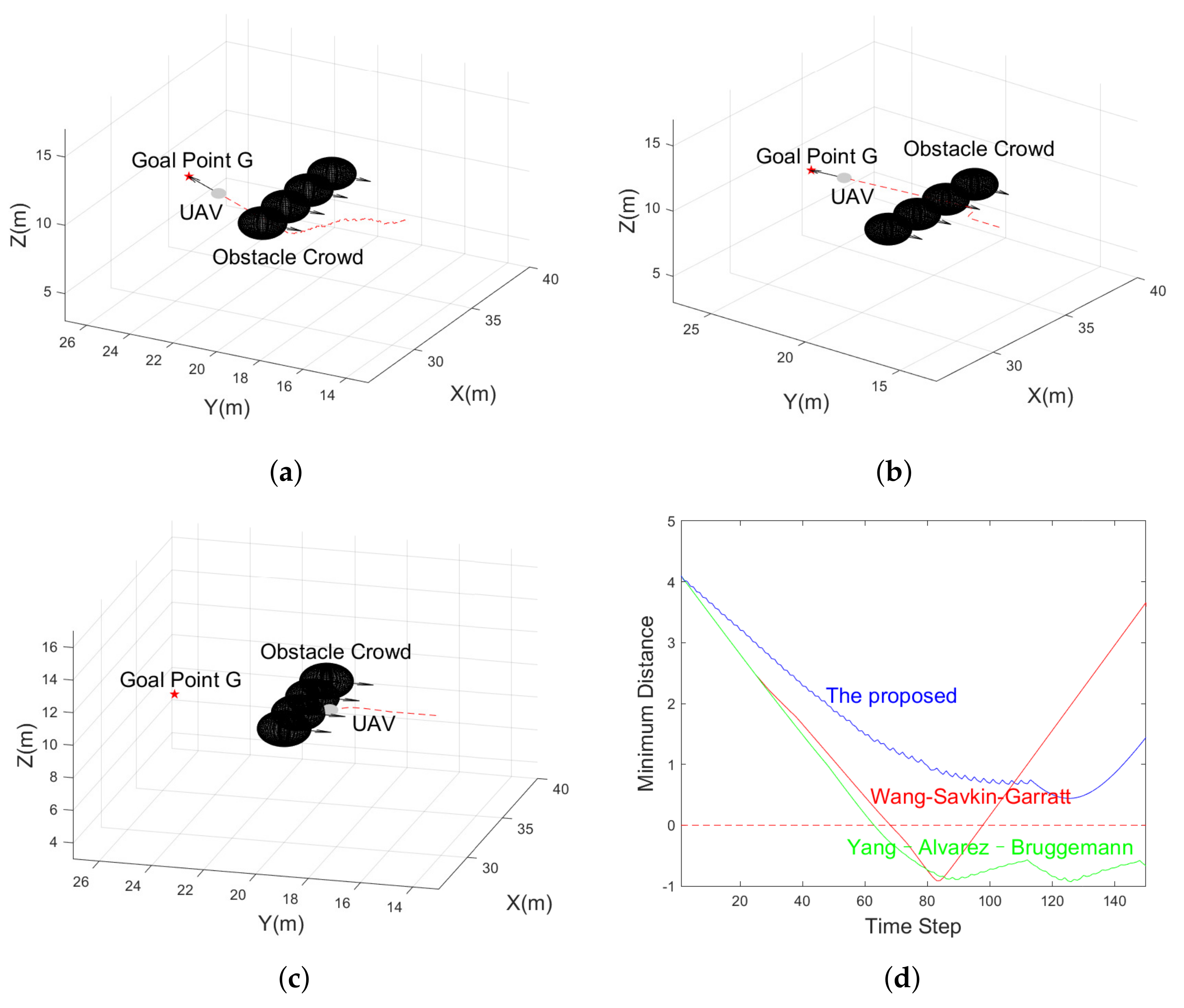
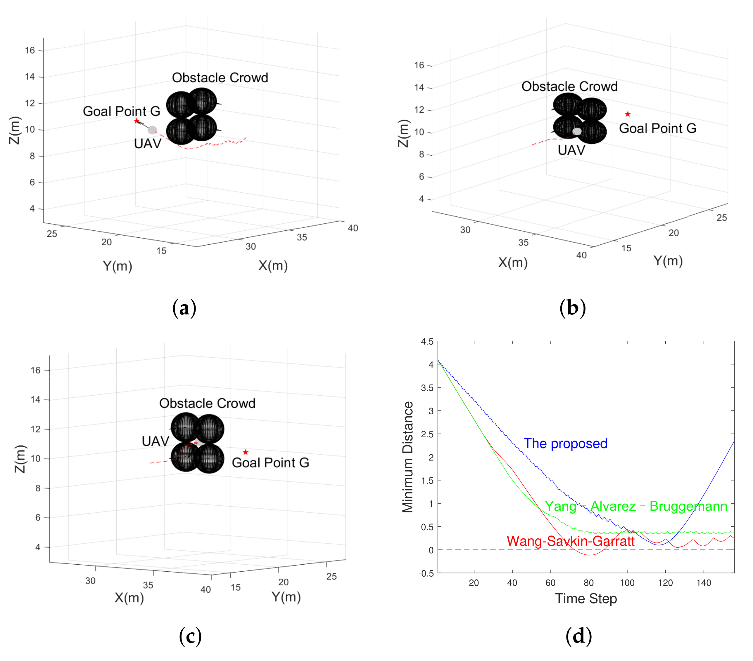
Two existing 3D navigation algorithms are simulated in different obstacles settings, and their drawbacks are pointed out.

(2)

A 3D vision cone-based navigation algorithm is proposed, enabling the UAV to seek a path through crowd-spaced obstacles in the unknown dynamic environments and non-cooperative scenarios.

(3)

Several simulations are conducted in MATLAB to compare the proposed algorithm with the other two state-of-the-art navigation algorithms in different unknown dynamic environments. As a result, the feasibility and superiority of the proposed 3D navigation algorithm are verified.

(4)

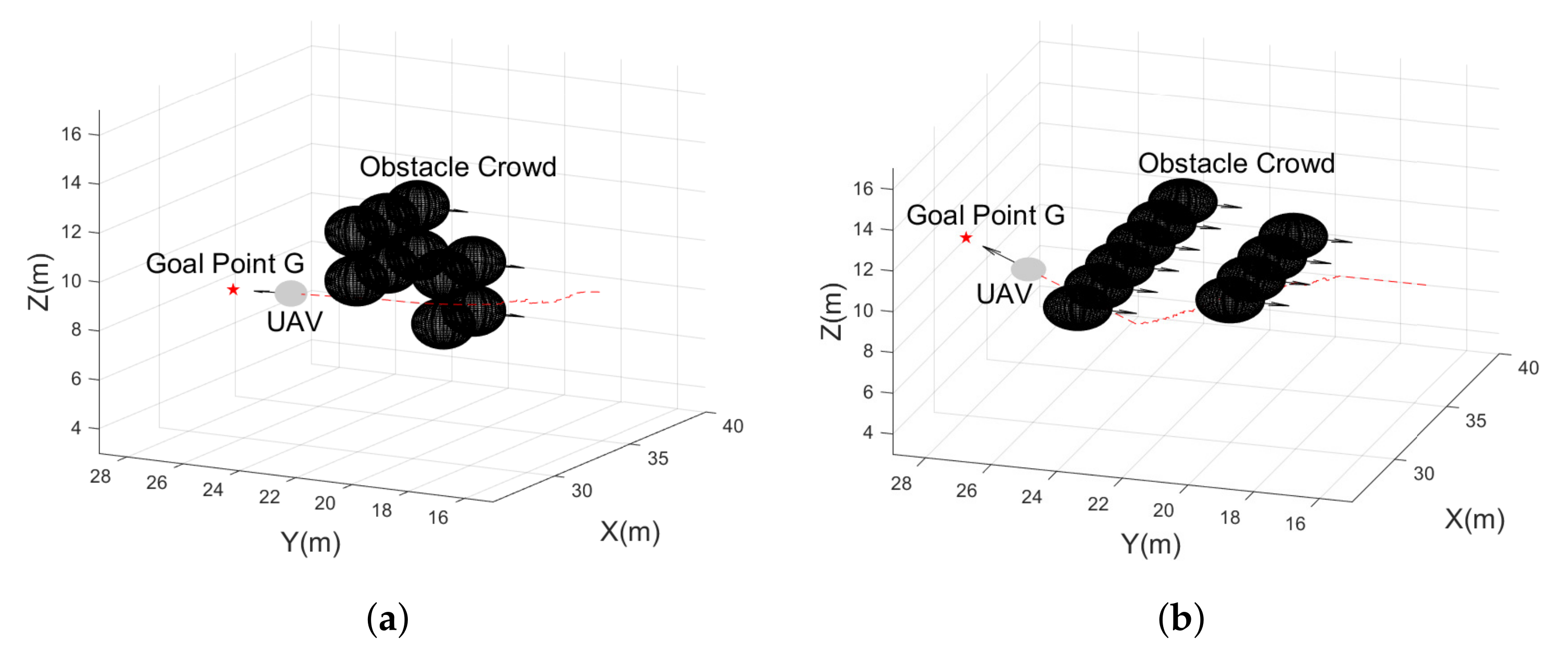
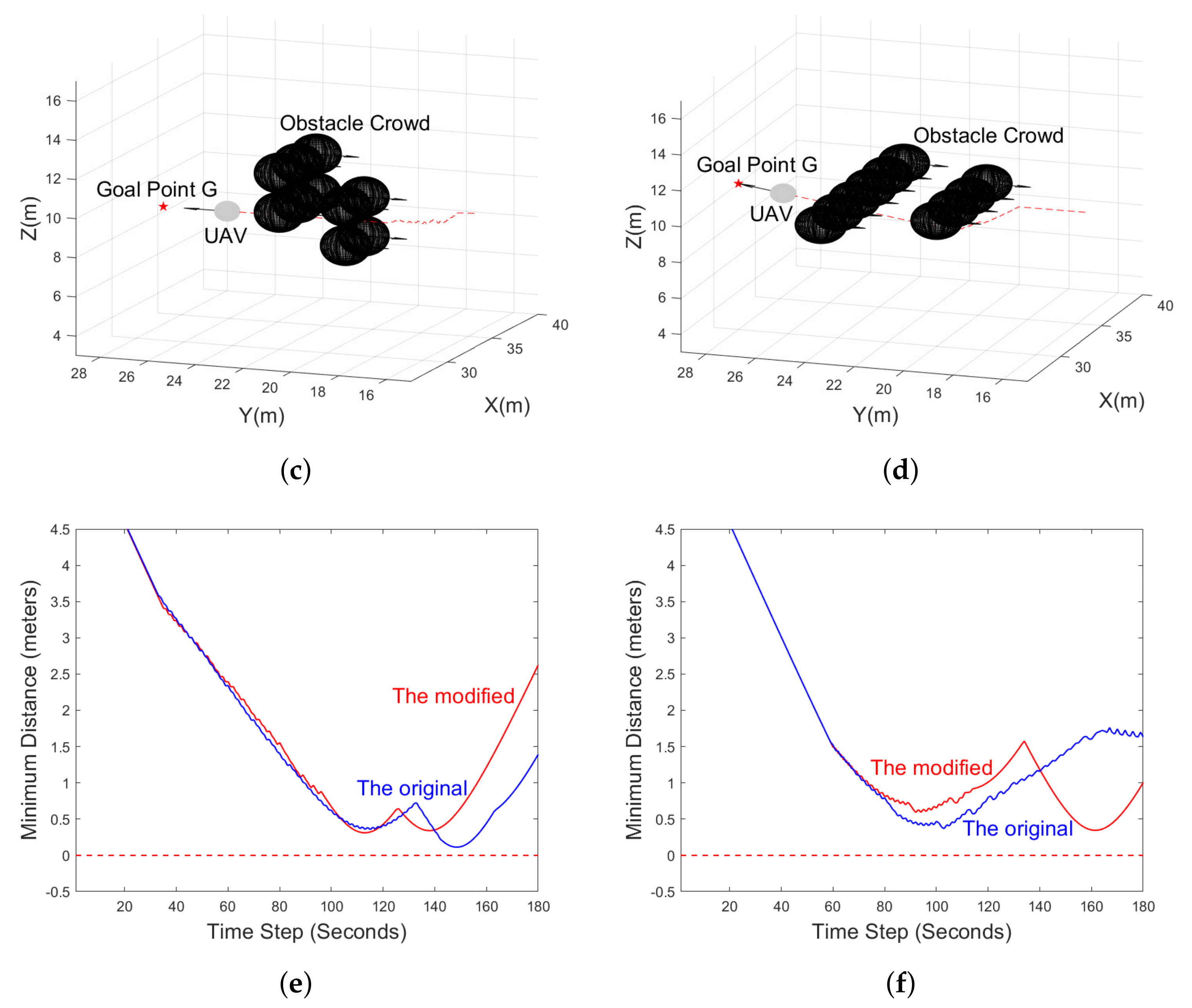
A modified idea of the proposed navigation algorithm is studied to improve the algorithm’s navigation performance further.

The rest of the paper is divided into six sections. Section 2 explains the background and introduces the existing literature in the 3D navigation domain. Section 3 presents the problem statement. Section 4 introduces the proposed navigation algorithm. Section 5 presents performance of the proposed algorithm via computer simulations. Moreover, comparisons with other 3D navigation algorithms are conducted to demonstrate the superiority of the proposed method. Finally, Section 6 gives the conclusion.

2. Related Work

In general, navigation algorithms can be divided into two categories. The first category is called the global planer, which is a map-level planer. It can figure out the shortest path or feasible path from a starting point to a destination point in the map. Classic algorithms in this domain are Dijkstra [30], A* [31], and RRT [32]. The second category is the local planer aiming at generating a feasible local collision-free path/direction to guide the UAV to avoid obstacles. The 3D local planer is our primary study object.

In [33], the authors propose a navigation potential field approach to bypass multiple obstacles simultaneously. In the paper, the authors first assume all the obstacles can be represented as cylinders, and the UAV’s altitude is fixed when doing obstacle avoidance maneuvers. This algorithm’s underlying idea is to use the navigation potential field to generate some new waypoints that can lead the UAV to bypass those detected obstacles simultaneously. Obviously, the advantage of this algorithm is that it can navigate the UAV to bypass multiple obstacles simultaneously. Still, this algorithm constrains the UAV’s altitude under evasive maneuvers, which removes one degree of freedom of the UAV. Moreover, when dealing with other flying objects in the outdoor environment, the cylinder representation of the obstacles occupies too much space in the vertical direction. Therefore, it makes the 3D space utility efficiency low.

In [34], the authors propose a novel cost function of the model predictive controller (MPC), which takes obstacle avoidance into consideration to generate the control input u to navigate the UAV. The optimal control signal is calculated through dynamic programming techniques embedded in the MPC over a finite receding horizon N. There are two matrix parameters in the MPC controller, Q, and R. The Q matrix is the state penalty matrix, and the R matrix is the input penalty matrix. Both matrixes represent the corresponding state’s weight during the optimization process. Thus, we can constrain a specific state or control signal by setting the corresponding elements in the Q or R matrix. The authors further improves the algorithm by introducing a dual-mode strategy. During a routine flight, the navigation algorithm will set the entries of parameter matrix Q and R to relatively large values to improve the destination point navigation performance. Once the potential collision is detected and the evasive maneuver is needed, the algorithm will set the entries of parameter matrix Q and R to a relatively small values to strengthen the obstacle avoidance performance. This algorithm’s advantage is that it can navigate the UAV to the destination point with collision-free and potentially bypass multiple obstacles simultaneously. Nevertheless, the MPC algorithm always suffers from the heavy calculation burden effect. If the algorithm wants to acquire a good real-time performance, the length of finite receding horizon N can not be very long. However, the short length of the receding horizon decreases the control performance. Thus, there exists a trade-off between the real-time performance and the quality of control input signal generation. Therefore, the sampling period between each step in the finite receding horizon and its total length must be carefully picked.

In [29], a collision-free navigation approach by maintaining a constant bearing and elevation angle concerning the closest obstacle is proposed. The underlying is that the algorithm first acquires the nearest obstacle’s position. A vector starting from UAV’s current position ending at the obstacle’s current position is obtained. Rotating this vector with respect to the x-axis and y-axis consecutively with the user preset angle to achieve the relative bearing and elevation angle maintain purpose. The obstacle avoidance performance heavily relies on the bearing and elevation angle settings. If both angles are set to a small values or the obstacle’s size is very large, the algorithm may fail to navigate the UAV to bypass the obstacles. Furthermore, when dealing with multiple obstacles, this algorithm fails to navigate the UAV to bypass crowd-placed obstacles in the space even if the bearing and elevation angle is set large enough.

In [28], a 2D-vision cone-based navigation algorithm is proposed. The authors use a covering sphere scheme to represent all the obstacles, and this representation allows the obstacle to deform or change its shape. The algorithm requires lots of prior knowledge regarding the obstacles, e.g., the velocity $v_i\left(t\right)$, and the position $x\left(t\right)$ of each obstacle. Based on the information, the algorithm will first identify the most dangerous obstacle, e.g., the closest one. Then, a pointing vector starting from the UAV’s current position ending at the picked obstacle’s current position is constructed. A 2D plane is constructed based on the UAV’s current motion direction vector a(t) and pointing vector. In this constructed 2D plane, the boundary of the 2D vision cone is calculated and generated. The two boundary vectors will be enlarged in the next stage to enable the UAV to bypass the obstacle. This algorithm has the same limitation as the one proposed in [29], which assumes a relatively large space between each obstacle, so the algorithm can navigate the UAV to bypass the obstacles one after another until the UAV reaches the final destination point. Once this assumption fails to hold in practice, the UAV will be tracked in a particular space or collide with the obstacles.

In [35], the authors use an RGB-D camera indoor supervision system combined with an onboard IMU sensor to acquire the obstacle’s position and measure the free space in the horizontal and vertical directions with respect to the current closest obstacles. The navigation control is straightforward. Once the free space in the horizontal and vertical direction is detected, the navigation control law will set a mid-target point to drive the UAV to that point to avoid the obstacle.

In [36], a hybrid navigation method is proposed to allow the UAV safe operation in partially unknown dynamic environments. The authors combine the global path planning algorithm called RRT-Connect with a SMC-based reactive control law to enable the UAV to avoid the obstacles efficiently. The performance of the proposed algorithm is verified in the MATLAB simulation with sparsely located static and dynamic obstacles. Nevertheless, this algorithm is never tested under crowd-spaced obstacles setting, and its safe navigation property is not guaranteed in this scenario.

In [37], an optimized transfer-convolutional neural network (CNN) approach based on an improved bat algorithm is proposed to safely navigate the UAV through the obstacles. Furthermore, to benefit from the automatic image classification technique applied to the algorithm, the training problem that supervised learning requires that a large amount of labeled data is solved. The resulting well-trained neural network achieved $94.84\%$ prediction accuracy on the test set announced by the authors. The camera array is installed on the top of the UAV to enhance its front environment perception capability. However, this navigation algorithm is only feasible when dealing with static obstacles. The proposed algorithm’s perception and obstacle avoidance capability needed to be further studied when facing dynamic obstacles.

In [38], a novel 3D local dynamic map (LDM) generation algorithm is proposed for the perception system of the UAV. The authors take memory usage and fast operation speed into consideration and use a circular buffer to implement this algorithm efficiently. The LDM is generated based on the sensor readings, position, and velocity estimated from the particle filter, and it keeps updating during the UAV flight. This 3D occupancy map generation algorithm indicated the vacancy space near the UAV well and gave the UAV a relatively accurate estimation of the obstacle’s velocity and position. However, its computation burden increases significantly when generating a large map to enhance the perception capability or using more particles to get better estimation, even though it uses an efficient data structure to implement.

In [39], a method that searches for obstacles across a cylindrical safety volume and finds an optimal escape point from a spiral for obstacle avoidance is proposed. The authors rely on a depth camera with a limited field of view and sensing range to generate a set of point clouds that are used to generate a map to reveal the near environment of the UAV. The resulting map representation is implemented on graphics processing unit (GPU) and central processing unit (CPU), respectively, to verify the real-time performance. A robust but straightforward navigation algorithm that uses a spiral is introduced to enable the UAV to achieve obstacle avoidance.

In [40], unlike the 3D occupancy map generation approaches for environment perception, this approach uses the object detection neural network to detect the drones. The authors tested a set of CNN-based object detection systems, such as Single Shot MultiBox Detector (SSD) with MobileNet v1 as backbone [41,42], Faster Region Based Convolutional Neural Networks (Faster-RCNN) [43], You Only Look Once v2 (YOLO v2) [44], and Tiny YOLO [45], to detect and track flying objects on the UAV’s current flying trajectory. However, due to the diversity constraint of the training data, the resulting network’s object detection accuracy cannot be guaranteed under all environments.

In recent years, reinforcement learning (RL) based approaches have been widely investigated in the UAV navigation domain [46,47,48,49,50,51,52,53,54]. The classic Q-learning (CQL) algorithm proposed in [55] has the underlying principle that when the UAV observes the environment information at time step k and takes actions based on the environment information obtained, an immediate reward can be obtained from the environment. This reward can either refer to collisions with the environment’s obstacles or bypassing the obstacles in the UAV navigation scenario. The goal of the CQL applied in the navigation is to navigate the UAV from the initial position to the destination point with maximum reward. One obvious advantage of the CQL is that it does not require any prior knowledge regarding the UAV’s current environment. CQL training process can be done by letting the UAV take action and gain reward in the environment. After training many times to make the CQL cost converge, the CQL-based approach can find the optimal path to navigate the UAV to bypass the obstacles. Nevertheless, during the training process of the CQL, a Q table is required to store the Q values from state to state, which makes the CQL hard to use when the UAV copes with a dynamic environment.

A neural Q learning (NQL) based approach is proposed in [51]. The authors combine the CQL with the Back Propagation Neural Network (BPN) to obtain the resulting NQL, which can be trained to achieve the obstacle avoidance purpose. There are two navigation control laws proposed in this algorithm. The first control law is called the fast approach policy used to navigate the UAV to the destination point directly when the obstacles are not detected. The second control law is NQL which is used as obstacles avoidance control law to navigate the UAV to bypass the obstacles when detected. The authors also briefly explore the difference between Deep Q Network (DQN), which is another RL and deep neural network (DNN) combined network, and NQL in their paper. In general, DQN has three different essential parts with NQL. Firstly, the CNN is used in DQN to extract the feature from images rather than using BPN to calculate Q values as in NQL. Hence, the input to the DQN is the image acquired from the on-board camera. Secondly, a training technique called the experience replay approach is adopted to train the DQN. Lastly, two Q networks exist in the DQN to achieve the obstacle avoidance and destination reaching.

In [52], a novel RL approach that combines the object detection network (ODN) with DQN is proposed. The authors point out the significant drawback of traditional deep reinforcement learning (DRL) that its prediction performance is not highly stable, which results in the UAV’s movement oscillate in the real-world application. Furthermore, to train the Deep Reinforcement Learning network (DRL), a specific image dataset is required. The well-trained DRL’s prediction performance may decrease significantly when the UAV operation environment is substantially different from the training dataset. Hence, an ODN+DQN scheme is proposed to solve the problems listed above. This scheme successfully reduces the flying time by $25\%$ and cut-down the unnecessary turns by $50\%$ announced by the author. Nevertheless, we have noticed that this algorithm is a 2D obstacle avoidance scheme developed from the UGVs scenario, and input states regarding the UAV’s coordination only contain x and y. Hence, the UAV’s altitude is fixed when doing obstacle avoidance operations.

The vast majority of the 3D navigation algorithms mentioned above either fixed the UAV’s altitude while doing obstacle avoidance or failed to bypass multiple crowd-spaced 3D obstacles simultaneously. In order to solve those limitations, we develop a novel 3D vision cone-based navigation method. The method we proposed can enable the UAV to conduct evasive maneuvers in any direction in a 3D environment rather than fixing the movement of the UAV in a specific 2D plane in 3D space. Moreover, it also enables the UAV to avoid multiple crowd-spaced obstacles simultaneously. A formal problem statement and 3D vision cone model are given in the following section, and the proposed method is presented in Section 4.

3. Problem Statement

In this paper, we study the under-actuated non-holonomic small quadcopter, and we further assume that the wind power is tiny in the UAV’s operation environment. Thus, the effect of the wind on the UAVs can be ignored. This assumption is valid when UAVs operate in an ample indoor space or outdoor space with good weather. Its mathematical model can be described as

$$P\left(t\right)=\left[x\left(t\right),y\left(t\right),z\left(t\right)\right]$$

(1)

which is the 3D vector UAV’s Cartesian coordinates. The motion of the UAV is described by the equation

$$v\left(t\right)=\dot{P}\left(t\right)=V\left(t\right)·a\left(t\right)$$

(2)

and

$$\dot{a}\left(t\right)=w\left(t\right)$$

(3)

In the above equations, $v\left(t\right)$ is the velocity vector of the UAV, $a\left(t\right)$ is the UAV’s motion direction. $V\left(t\right)$ and $w\left(t\right)$ are the control inputs, $V\left(t\right)$ is the scalar variable refers to the linear velocity of the UAV, $w\left(t\right)$ is applied to change the direction of the UAV’s motion. The kinematic model represented in Equations (1)–(3) was first proposed in [56], and rigorous mathematical analysis has been conducted to verify its viability to represent many unmanned aerial and underwater vehicles. We adopt this model to perform simulation coding and algorithm development in the rest of the paper. Furthermore, we require the following constraints hold.

$$∥a\left(t\right)∥=1$$

(4)

$$∥w\left(t\right)∥⩽W_{max}$$

(5)

$$V\left(t\right)\in \left[V_{min},V_{max}\right]$$

(6)

$$⟨a\left(t\right),w\left(t\right)⟩=0$$

(7)

Here, $∥·∥$ denotes the L2 norm operator, $⟨·,·⟩$ denotes the inner product operator. The scalar variables $W_{max}$, $V_{min}$, and $V_{max}$ are determined based on the performance of each UAV.

We study a quite general three-dimensional problem of autonomous vehicle navigation with collision avoidance. In particular, we assume that there are several disjoint moving obstacles and a stationary final destination point G in the 3D space. The objective is to drive the UAV to this final destination point while avoiding collisions with the moving obstacles. We assume that all obstacles are always inside some moving sphere of a known radius constructed by the UAV’s navigation system, those spheres are said to be the covering sphere of the obstacles, and the minimum distance from any obstacles to the UAV as well as their velocities are unknown, but any obstacle’s velocity $v_i\left(t\right)$ must satisfy the constraint:

$$v_i\left(t\right)<V_{obs}<V_{max}$$

(8)

In inequality (8), the $V_{obs}$ refers to the maximum velocity that obstacles can reach, and UAV knows the coordinate of the goal point G. Obviously, only condition (8) meets, then our UAV is capable of avoiding the obstacles safely.

In order to detect 3D space obstacles and perceive the UAV’s front environment, several 3D vision cones are adopted with a depth camera, where each 3D vision cone is acquired by drawing a circle on the depth map that the depth camera returned. Each circle’s boundary is divided into M pixels, and each pixel coordinate in the world frame serves as the end of the boundary of each 3D vision cone. The perception capability of each 3D vision cone can be improved with more M pixels, but the computation burden increases as well. Therefore, there is a trade-off between perception capability determined by the number of 3D vision cones, boundaries and computation burden. The vision cones are exhibited in Figure 1.

Figure 1. Three-dimensional vision cones.

Each 3D vision cone shares the same height, and each boundary of the 3D vision cone will check the intersect with the obstacles to find the vacant space, which will lead the UAV to conduct obstacle avoidance. Furthermore, the inner structure of each 3D vision cone can be described by using Figure 2.

Figure 2. Inner structure of 3D vision cone. $\theta$: the apex angle of the 3D vision cone. l: the length of the boundary of this 3D vision cone. h: the height of this 3D vision cone. r: the radius of the bottom circle of this 3D vision cone.

We denote $\theta$ as the apex angle, l refers to the boundary length, h is the height of the 3D vision cone and is determined by the capability of the depth camera, and r is the radius of the bottom circle. It is worth noting that once the apex angle $\theta$ and height h are specified, the other two parameters are also determined. Moreover, the apex angle serves as the range-sensing angle, which spanned over the interval [$0^{\circ }$, ${90}^{\circ }$) to acquire all the environment information in front of the UAV. Nevertheless, in practice, due to physical constraints, the angle sensing range is much smaller. The user can define the total number of 3D vision cones as long as the outermost 3D vision cone is within the sensor’s sensing range. That is, each UAV has a maximum apex angle and its associate 3D vision cone due to the physical constraint of the sensor. In our case, we only define four vision cones to simplify the simulation process and make it easy to represent the idea. After defining the outermost 3D vision cone, the number of inner 3D vision cones can be arbitrarily large depending on the users’ navigation requirements, such as a more accurate avoidance trajectory or an avoidance trajectory with less control effort. In our simulation, we pick $\theta$ equals to $5^{\circ }$, ${10}^{\circ }$, ${15}^{\circ }$, and ${20}^{\circ }$ to construct the four 3D vision cones used to detect the obstacles.

Furthermore, due to the physical constraint of the field of view of the camera, the obstacle with large volume beyond the outermost 3D vision cone’s sensing range will cause the proposed algorithm to fail to find an optimal motion direction, and this scenario is well demonstrated in Figure 3. Therefore, we assume that all obstacles should have a volume that is smaller than the outermost 3D vision cone’s sensing range to ensure the proposed algorithm can operate well in the unknown dynamic environments.

Figure 3. Obstacle with large volume beyond the outermost 3D vision cone’s sensing range.

This study aims to develop a destination reaching with collision avoidance navigation strategy for UAVs where only limited obstacles’ information is available. The proposed algorithm exhibited in the next section is a local planer rather than a global planer that navigates the UAVs in the unknown dynamic environments.

4. 3D Vision Cone-Based UAV Navigation Algorithm

The proposed navigation algorithm consists of two control laws: (1) 3D vision cone-based obstacle avoidance control law and (2) destination reaching control law. The switching condition between two control laws is that when all 3D vision cones do not detect any obstacles, the destination reaching control law is executed to drive our UAV to the destination point G. Nevertheless, once the 3D vision cones detect any obstacles, the obstacle avoidance control law is invoked to drive the UAV to bypass any detected obstacles until all the 3D vision cones no longer see any obstacles.

4.1. 3D Vision Cone-Based Obstacle Avoidance Control Law

As mentioned at the end of Section 3 we adopt four vision cones to find the vacant space and determine the optimal motion direction of the UAV. Each boundary segment on the 3D vision cone will be used to detect the free space in its current heading direction. The intersection condition of each boundary segment with any stationary or moving obstacles will be checked and recorded. The following example explains the detailed procedure to generate the optimal motion direction from those 3D vision cones when facing crowd-spaced obstacles.

Figure 4 corresponds to the intersection condition exhibited in Figure 1. Value 1 indicates that the corresponding boundary has no intersection with any obstacles, and value 0 shows the corresponding boundary has an intersection with the obstacles and the direction of that boundary heading is not vacant. The user can determines the number of boundaries of each 3D vision cone. More boundaries will result in better optimal motion direction, but the computation burden of the proposed algorithm will increase; it’s a tunable parameter. In our case, we choose 100 boundaries to make it easy to represent our ideas. Since all 3D vision cones have a bottom circle, each boundary can be identified as the vertices on the bottom circle connected to the vertex of the 3D cone. We use polar coordinates to give the sequence of each boundary starting from 0 degrees on the x-axis to 360 degrees counterclockwise, and this process is exhibited in Figure 5. Thus, each neighbored boundary has a polar angle difference equal to 360/100 degrees.

Figure 4. Intersection condition of each 3D vision cone.

Figure 5. Boundary sequence generation process. 1 refers to 1th boundary, 2 refers to 2th boundary, 3 refers to 3th boundary, 4 refers to the 4th boundary, $\mathsf{\alpha }$: the difference angle between each boundary projected on the bottom circle.

According to the information shown in Figure 4, there are eight free intervals in total. The optimal motion direction $a_{opt}$ is generated by first checking the most inner 3D vision cone’s boundaries to find the boundaries that have no intersection with obstacles. In our case, since all boundaries of the most inner 3D vision cone have intersected with obstacles, we move to the second most inner 3D vision cone and check the intersection condition of its boundaries. Once an interval formed of vacant boundaries is found, we will measure its length and compare it with other intervals that come from the same 3D vision cone. Once the free interval with the longest length is identified, we choose the intermediate boundary from this longest free interval. Then, we normalize this chosen boundary and let it be the UAV’s optimal motion direction $a_{opt}$. Since the neighbor boundaries of the chosen boundary are all from the same longest free interval in the same 3D vision cone and have no intersection with any obstacles, this chosen boundary is pointing toward the middle of the vacant space. Therefore, it can be used as the desired motion direction to navigate our UAV bypass the obstacle crowd.

After an optimal UAV’s motion direction $a_{opt}\left(t\right)$ is determined, a sliding mode controller (SMC), which is the derivative of the controller proposed in [28], is adopted to drive the UAVs toward this optimal UAV’s motion direction. The control input $w\left(t\right)$ is calculated through the equation

$$w\left(t\right)=W_{max}·H\left(a\left(t\right),a_{opt}\left(t\right)\right)$$

(9)

and

$$H\left(a_1,a_2\right)=\left\{\begin{array}{cc}0\hfill & h\left(a_1,a_2\right)=0\hfill \\ \frac{h\left(a_1,a_2\right)}{∥h\left(a_1,a_2\right)∥}\hfill & h\left(a_1,a_2\right)\ne 0\hfill \end{array}\right.$$

(10)

$$h\left(a_1,a_2\right)=a_2-⟨a_1,a_2⟩·a_1$$

(11)

Function H in Equations (9) and (10) takes two 3D vectors, $a_1$ and $a_2$ as input, and generates a 3D vector that is orthogonal to the input vector $a_1$ and pointing toward the second input vector $a_2$, as output. The relationship between two input 3D vectors and one output 3D vector is well exhibited in Figure 6. In our case, $a_1=a\left(t\right)$, which is our UAV’s current motion direction, and $a_2=a_{opt}\left(t\right)$, which is our UAV’s optimal motion direction, can guide UAV to do obstacle avoidance or destination reaching. Therefore, it ensures the generated control input $w\left(t\right)$ will drive the UAV’s current motion direction $a\left(t\right)$ toward the optimal direction $a_{opt}\left(t\right)$. As for another control input $V\left(t\right)$, it is a tunable scalar parameter that should be picked in the range $\left(V_{obs},V_{max}\right]$.

Figure 6. Relationship between $H\left(a_1,a_2\right)$ and $a_1$, $a_2$.

4.2. Destination Reaching Control Law

Under destination reaching control law, the control input $w\left(t\right)$ is calculated based on the Equation (5) with modified content as

$$w\left(t\right)=W_{max}·H\left(a\left(t\right),b\left(t\right)\right)$$

(12)

$$b\left(t\right)=\frac{G-P\left(t\right)}{∥G-P\left(t\right)∥}$$

(13)

In this case, $b\left(t\right)$, which is the vector heading toward the final destination 3D point, becomes the optimal motion vector for the UAV. Besides, due to the fact that there are no obstacles that threaten our UAV under this control law, another control input $V\left(t\right)$ is set to be $V\left(t\right)=V_{max}$ to navigate the UAV to the destination as fast as possible.

Based on the two control laws given in Section 4.1 and Section 4.2, when any obstacles getting close to the UAV, 3D vision cones will first detect those obstacles and find an optimal motion direction that indicates the vacant space. Then, a sliding mode controller will take this optimal motion direction vector and the UAV’s current motion direction vector as inputs and generate a control signal as output. The control signal will then be applied to change the UAV’s current motion direction toward that optimal motion direction to achieve obstacle avoidance. Finding the optimal motion direction and generating the control signal will keep going until all 3D vision cones no longer detect any obstacles, which means the UAV has successfully avoided all the obstacles that the 3D vision cones detected before. At this moment, there are no more obstacles that threaten our UAV’s safety. So, the destination reaching law in Section 4.2 will be executed, which uses the same sliding mode controller in Section 4.1 to generate the control signal that navigates the UAV to the final destination until the 3D vision cones detect new obstacles or the final destination point is reached. The execution logic of the proposed navigation algorithm is well exhibited as a flowchart in Figure 7.

Figure 7. Flowchart of proposed navigation algorithm.

We will further demonstrate the effectiveness of the proposed approach via extensive computer simulations and conduct a comparison study against other methods in the following section.

5. Computer Simulation Results

We demonstrate the performance of the proposed 3D vision cone-based navigation algorithm with MATLAB simulation. In our simulation, we set sampling rate $∆T=0.1$ second, the height of each 3D vision cone $h=3.5$ m, and four 3D vision cones with apex angles $5^{\circ }$, ${10}^{\circ }$, ${15}^{\circ }$, ${20}^{\circ }$, respectively. At the very beginning, we start with a simple scenario where the UAV tries to bypass a single obstacle, as shown in Figure 8.

Figure 8. UAV bypass single obstacle. (a) Simulation initial setup. (b) Switch from navigation to avoidance. (c) Switch from avoidance to navigation. (d) Destination reaching. (e) Distance between obstacle and UAV.

Figure 8a shows the initial setup of the simulation. In Figure 8b, four 3D vision cones are depicted and used to represent that the UAV perceives the existence of the obstacle. Then, the proposed navigation algorithm is executed to find the optimal UAV motion direction and drive the UAV toward that direction to bypass the obstacle. After the obstacle is successfully bypassed, destination reaching law is invoked to drive the UAV moves toward the final destination point G as depicted in Figure 8c,d. Figure 8e shows the distance between the obstacle and UAV, and it indicates there is no collision with the obstacle. This simulation demonstrates that the proposed 3D vision cone-based navigation algorithm is capable of maintaining a safe distance between UAV and obstacle and drive the UAV to the final destination.

In Figure 9, the proposed navigation algorithm is tested in a more challenging scenario where the UAV tries to reach the goal point while avoiding multiple moving obstacles.

Figure 9. UAV bypasses multiple obstacles. (a) Simulation initial setup. (b) Simulation result at time step 160. (c) Simulation result at time step 260. (d) Destination reaching. (e) Top View. (f) Minimum distance between obstacles and UAV.

Figure 9a exhibit the initial setup, Figure 9b,d exhibit the significant moments when the UAV bypass the obstacles. Figure 9e exhibit the top view of the whole trajectory. Figure 9f shows the minimum distance between the closest obstacle and UAV, and it demonstrates that there is no collision with any obstacles. These simulations again verify that the proposed navigation algorithm can keep a safe distance to the obstacle even in a challenging environment with multiple moving obstacles.

Finally, we compare the performance of the proposed 3D vision cone-based navigation algorithm with Wang–Savkin–Garratt algorithm [28] and Yang–Alvarez–Bruggemann algorithm [29] in two different crowd-spaced obstacles scenarios. The simulation results will verify that our proposed 3D navigation algorithm can seek a path through crowd-spaced obstacles and outperform these two algorithms.

Figure 10a shows that the proposed 3D vision cone-based navigation algorithm successfully found a path to avoid those four moving obstacles simultaneously. In contrast, Wang–Savkin–Garratt algorithm [28] is failed to bypass the crowd-spaced obstacles and collide with one of the obstacles, exhibited in Figure 10b. Figure 10c represents the simulation result of the Yang–Alvarez–Bruggemann algorithm [29], again it failed to navigate the UAV to bypass those four obstacles and make the UAV collide with one of the obstacles. Figure 10d shows the minimum distance between the UAV and the closest obstacle among the four during the navigation. We can observe from Figure 10 that the proposed 3D navigation algorithm never collides with any obstacles and successfully drive the UAV to move away from the obstacles. In contrast, the Wang–Savkin–Garratt algorithm [28] and the Yang–Alvarez–Bruggemann algorithm [29] propelled the UAV to collide with the obstacles multiple times and failed to drive the UAV to reach the destination point in this scenario.

Figure 10. UAV facing crowd-spaced obstacles. (a) The proposed algorithm. (b) Wang–Savkin–Garratt algorithm [28]. (c) Yang–Alvarez–Bruggemann algorithm [29]. (d) Minimum distance between obstacles and UAV.

In Figure 11, a different crowd-spaced obstacles are presented to test the performance of each 3D navigation algorithms.

Figure 11. UAV facing another crowd-spaced obstacles. (a) The proposed algorithm. (b) Wang–Savkin–Garratt algorithm [28]. (c) Yang–Alvarez–Bruggemann algorithm [29]. (d) Minimum distance between obstacles and UAV.

Again, Figure 11a shows that the proposed 3D navigation algorithm successfully found a path to avoid those four moving obstacles simultaneously with collision-free. However, the Wang–Savkin–Garratt algorithm [28] is failed to bypass the crowd-spaced obstacles and collide with one of the obstacles, exhibited in Figure 11b. Figure 11c represents the simulation result of the Yang–Alvarez–Bruggemann algorithm [29], it did not make the UAV collide with any obstacles but made the UAV tracked in the specific position. Figure 11d shows the minimum distance between the UAV and the closest obstacle among the four during the navigation. Furthermore, it proves the previous analysis.

During the simulation, we discovered that the performance of the proposed 3D vision cone-based navigation algorithm could be further improved by modifying the switching condition of two control laws. As long as the innermost 3D vision cone no longer detects any obstacles, the destination reaching control law is executed to navigate the UAV to the goal point G. We assume that the radius of the bottom circle of the innermost 3D vision cone is larger than the UAV covering sphere to ensure the safe navigation. The navigation performance of the modified version of the proposed algorithm is compared with the initially proposed algorithm shown in Figure 12.

Figure 12. Performance comparison of the original and modified versions of the proposed algorithm. (a) The proposed algorithm. (b) The proposed algorithm. (c) The modified proposed algorithm. (d) The modified proposed algorithm. (e) Minimum distance between obstacles and UAV. (f) Minimum distance between obstacles and UAV.

Figure 12a,b exhibit the simulation result of the originally proposed algorithm in two different crow-spaced obstacles scenarios. Furthermore, there is an obvious left turn in two scenarios that make the UAV travel more space to bypass the obstacle crowd. In contrast, Figure 12c,d exhibit the simulation result of the modified version of the proposed algorithm, and it drives the UAV to travel a more efficient path and get to the goal point G faster than the originally proposed algorithm. Figure 12e,f represents the minimum distance between the UAV and obstacles under two navigation algorithms driven and in two different obstacle crowd scenarios, respectively. Those two figures verify that the modified algorithm makes the UAV fly away from the obstacles faster than the initially proposed algorithm. However, the risk of colliding with obstacles is increased under specific scenarios. Thus, there exists a trade-off between travel efficiency and safe obstacle avoidance, and worth study in the future.

Furthermore, we simulate our proposed and modified navigation algorithms in a more complex environment, where multiple crowd-spaced obstacles exist, to demonstrate their obstacles avoidance performance. The simulation result is well exhibited in Figure 13.

Figure 13. Performance of the original and modified versions of the proposed algorithm in multiple crowd-spaced obstacles environment. (a) The proposed algorithm. (b) The proposed algorithm. (c) The modified proposed algorithm. (d) The modified proposed algorithm. (e) The minimum distance between obstacles and UAV. (f) The minimum distance between obstacles and UAV.

Figure 13e,f represent the minimum distance between UAV and obstacles under two navigation algorithms driven and in two different obstacle crowd scenarios, respectively. Those two figures verify that both navigation algorithms can navigate the UAV to bypass multiple crowd-spaced obstacles without collisions as long as the volume of the crowd-spaced obstacles is within the outermost 3D vision cone’s sensing range.

6. Conclusions

In this paper, a 3D vision cone-based reactive navigation algorithm and its modified version are proposed to enable a UAV to seek a path through the crowd-spaced 3D obstacles to the destination without collisions. The proposed algorithm is first simulated in MATLAB with several different 3D obstacles settings to demonstrate its feasibility. Then, we compared our proposed algorithm with Wang–Savkin–Garratt algorithm [28] and Yang–Alvarez–Bruggemann algorithm [29]. Both algorithms are state-of-the-art collision-free 3D navigation algorithms that can only avoid obstacles one at a time and cannot avoid multiple obstacles simultaneously. Therefore, the UAVs that navigate under these two algorithms may lead to collision when facing crowd-spaced obstacles. We simulated and compared our proposed navigation algorithm with these two in a crow-spaced obstacle environment to prove the superiority of our proposed algorithm when facing densely placed obstacles in a 3D environment. Moreover, the modified version of the proposed algorithm, which changes the switching condition between two control laws, is compared with the initially proposed algorithm to reveal the potential performance improvement strategy and lay the foundation for future work.

References

1. Xiang, W.; Xinxin, W.; Jianhua, Z.; Jianchao, F.; Xiu and, S.; Dejun, Z. Monitoring the thermal discharge of hongyanhe nuclear power plant with aerial remote sensing technology using a UAV platform. In Proceedings of the 2017 IEEE International Geoscience and Remote Sensing Symposium (IGARSS), Fort Worth, TX, USA, 23–28 July 2017; pp. 2958–2961. [Google Scholar] [CrossRef]
2. Li, X.; Savkin, A.V. Networked Unmanned Aerial Vehicles for Surveillance and Monitoring: A Survey. Future Internet 2021, 13, 174. [Google Scholar] [CrossRef]
3. Zhang, J.; Huang, H. Occlusion-Aware UAV Path Planning for Reconnaissance and Surveillance. Drones 2021, 5, 98. [Google Scholar] [CrossRef]
4. de Moraes, R.S.; de Freitas, E.P. Multi-UAV Based Crowd Monitoring System. IEEE Trans. Aerosp. Electron. Syst. 2020, 56, 1332–1345. [Google Scholar] [CrossRef]
5. Moranduzzo, T.; Melgani, F. Monitoring structural damages in big industrial plants with UAV images. In Proceedings of the 2014 IEEE Geoscience and Remote Sensing Symposium, Quebec City, QC, Canada, 13–18 July 2014; pp. 4950–4953. [Google Scholar] [CrossRef]
6. Marinov, M.B.; Topalov, I.; Ganev, B.; Gieva, E.; Galabov, V. UAVs Based Particulate Matter Pollution Monitoring. In Proceedings of the 2019 IEEE XXVIII International Scientific Conference Electronics (ET), Sozopol, Bulgaria, 12–14 September 2019; pp. 1–4. [Google Scholar] [CrossRef]
7. Gupta, M.; Abdelsalam, M.; Khorsandroo, S.; Mittal, S. Security and Privacy in Smart Farming: Challenges and Opportunities. IEEE Access 2020, 8, 34564–34584. [Google Scholar] [CrossRef]
8. Lottes, P.; Khanna, R.; Pfeifer, J.; Siegwart, R.; Stachniss, C. UAV-based crop and weed classification for smart farming. In Proceedings of the 2017 IEEE International Conference on Robotics and Automation (ICRA), Singapore, 29 May–3 June 2017; pp. 3024–3031. [Google Scholar] [CrossRef]
9. Tokekar, P.; Hook, J.V.; Mulla, D.; Isler, V. Sensor Planning for a Symbiotic UAV and UGV System for Precision Agriculture. IEEE Trans. Robot. 2016, 32, 1498–1511. [Google Scholar] [CrossRef]
10. Reddy, P.K.; Hakak, S.; Alazab, M.; Bhattacharya, S.; Gadekallu, T.R.; Khan, W.Z.; Pham, Q. Unmanned Aerial Vehicles in Smart Agriculture: Applications, Requirements, and Challenges. IEEE Sens. J. 2021, 21, 17608–17619. [Google Scholar] [CrossRef]
11. Khosravi, M.; Pishro-Nik, H. Unmanned Aerial Vehicles for Package Delivery and Network Coverage. In Proceedings of the 2020 IEEE 91st Vehicular Technology Conference (VTC2020-Spring), Antwerp, Belgium, 25–28 May 2020; pp. 1–5. [Google Scholar] [CrossRef]
12. Sawadsitang, S.; Niyato, D.; Tan, P.; Wang, P. Joint Ground and Aerial Package Delivery Services: A Stochastic Optimization Approach. IEEE Trans. Intell. Transp. Syst. 2019, 20, 2241–2254. [Google Scholar] [CrossRef] [Green Version]
13. Huang, H.; Savkin, A.V.; Huang, C. Round Trip Routing for Energy-Efficient Drone Delivery Based on a Public Transportation Network. IEEE Trans. Transp. Electrif. 2020, 6, 1368–1376. [Google Scholar] [CrossRef]
14. Sawadsitang, S.; Niyato, D.; Tan, P.S.; Wang, P. Supplier Cooperation in Drone Delivery. In Proceedings of the 2018 IEEE 88th Vehicular Technology Conference (VTC-Fall), Chicago, IL, USA, 27–30 August 2018; pp. 1–5. [Google Scholar] [CrossRef] [Green Version]
15. Liu, X.; Ansari, N. Resource Allocation in UAV-Assisted M2M Communications for Disaster Rescue. IEEE Wirel. Commun. Lett. 2019, 8, 580–583. [Google Scholar] [CrossRef]
16. Liang, Y.; Xu, W.; Liang, W.; Peng, J.; Jia, X.; Zhou, Y.; Duan, L. Nonredundant Information Collection in Rescue Applications via an Energy-Constrained UAV. IEEE Internet Things J. 2019, 6, 2945–2958. [Google Scholar] [CrossRef]
17. Atif, M.; Ahmad, R.; Ahmad, W.; Zhao, L.; Rodrigues, J.J. UAV-Assisted Wireless Localization for Search and Rescue. IEEE Syst. J. 2021, 15, 3261–3272. [Google Scholar] [CrossRef]
18. Aiello, G.; Hopps, F.; Santisi, D.; Venticinque, M. The Employment of Unmanned Aerial Vehicles for Analyzing and Mitigating Disaster Risks in Industrial Sites. IEEE Trans. Eng. Manag. 2020, 67, 519–530. [Google Scholar] [CrossRef]
19. Matveev, A.S.; Wang, C.; Savkin, A.V. Real-time navigation of mobile robots in problems of border patrolling and avoiding collisions with moving and deforming obstacles. Robot. Auton. Syst. 2012, 60, 769–788. [Google Scholar] [CrossRef]
20. Low, E.M.P.; Manchester, I.R.; Savkin, A.V. A biologically inspired method for vision-based docking of wheeled mobile robots. Robot. Auton. Syst. 2007, 55, 769–784. [Google Scholar] [CrossRef]
21. Hoy, M.C.; Matveev, A.S.; Savkin, A.V. Algorithms for collision-free navigation of mobile robots in complex cluttered environments: A Survey. Robotica 2018, 33, 463–497. [Google Scholar] [CrossRef] [Green Version]
22. Matveev, A.S.; Savkin, A.V.; Hoy, M.C.; Wang, C. Safe Robot Navigation among Moving and Steady Obstacles; Elsevier: Amsterdam, The Netherlands, 2015. [Google Scholar]
23. Savkin, A.V.; Wang, C. Seeking a path through the crowd: Robot navigation in unknown dynamic environments with moving obstacles based on an integrated environment representation. Robot. Auton. Syst. 2014, 62, 1568–1580. [Google Scholar] [CrossRef]
24. Hernandez, J.D.; Vidal, E.; Vallicrosa, G.; Galceran, E.; Carreras, M. Online path planning for autonomous underwater vehicles in unknown Environments. In Proceedings of the IEEE International Conference on Robotics and Automation (ICRA), Seattle, WA, USA, 26–30 May 2015; pp. 1152–1157. [Google Scholar]
25. Tordesillas, J.; How, J.P. MADER: Trajectory planner in multiagent and dynamic environments. IEEE Trans. Robot. 2021. [Google Scholar] [CrossRef]
26. Munoz, F.; Espinoza, E.; Gonzalez, I.; Garcia Carrillo, L.; Salazar, S.; Lozano, R. A UAS obstacle avoidance strategy based on spiral trajectory tracking. In Proceedings of the International Conference on Unmanned Aircraft Systems, Denver, CO, USA, 9–12 June 2015; pp. 593–600. [Google Scholar]
27. Li, H.; Savkin, A.V. Wireless Sensor Network Based Navigation of Micro Flying Robots in the Industrial Internet of Things. IEEE Trans. Ind. Inform. 2018, 14, 3524–3533. [Google Scholar] [CrossRef]
28. Wang, C.; Savkin, A.; Garratt, M. A strategy for safe 3D navigation of non-holonomic robots among moving obstacles. Robotica 2018, 36, 275–297. [Google Scholar] [CrossRef]
29. Yang, X.; Alvarez, L.M.; Bruggemann, T. A 3D Collision Avoidance Strategy for UAVs in a Non-Cooperative Environment. J. Intell. Robot Syst. 2013, 70, 315–327. [Google Scholar] [CrossRef] [Green Version]
30. Dijkstra, E. A note on two problems in connexion with graphs. Numer. Math. 1959, 1, 269–271. [Google Scholar] [CrossRef] [Green Version]
31. Hart, P.E.; Nilsson, N.J.; Raphael, B. A Formal Basis for the Heuristic Determination of Minimum Cost Paths. IEEE Trans. Syst. Sci. Cybern. 1968, 4, 100–107. [Google Scholar] [CrossRef]
32. LaValle, S.M. Rapidly-Exploring Random Trees: A New Tool for Path Planning; Technical Report; Computer Science Department, Iowa State University: Ames, IA, USA, 1998. [Google Scholar]
33. Salau, B.; Challoo, R. Multi-obstacle avoidance for UAVs in indoor applications. In Proceedings of the 2015 International Conference on Control Instrumentation, Communication and Computational Technologies (ICCICCT), Kumaracoil, India, 18–19 December 2015; pp. 786–790. [Google Scholar] [CrossRef]
34. Shim, D.H.; Sastry, S. An Evasive Maneuvering Algorithm for UAVs in See-and-Avoid Situations. In Proceedings of the 2007 American Control Conference, New York, NY, USA, 9–13 June 2007; pp. 3886–3891. [Google Scholar] [CrossRef]
35. Santos, M.C.P.; Santana, L.V.; Brandão, A.S.; Sarcinelli-Filho, M. UAV obstacle avoidance using RGB-D system. In Proceedings of the 2015 International Conference on Unmanned Aircraft Systems (ICUAS), Denver, CO, USA, 9–12 June 2015; pp. 312–319. [Google Scholar] [CrossRef]
36. Elmokadem, T.; Savkin, A.V. A Hybrid Approach for Autonomous Collision-Free UAV Navigation in 3D Partially Unknown Dynamic Environments. Drones 2021, 5, 57. [Google Scholar] [CrossRef]
37. Wang, S.; Wang, L.; He, X.; Cao, Y. A Monocular Vision Obstacle Avoidance Method Applied to Indoor Tracking Robot. Drones 2021, 5, 105. [Google Scholar] [CrossRef]
38. Lee, J.-W.; Lee, W.; Kim, K.-D. An Algorithm for Local Dynamic Map Generation for Safe UAV Navigation. Drones 2021, 5, 88. [Google Scholar] [CrossRef]
39. Azevedo, F.; Cardoso, J.S.; Ferreira, A.; Fernandes, T.; Moreira, M.; Campos, L. Efficient Reactive Obstacle Avoidance Using Spirals for Escape. Drones 2021, 5, 51. [Google Scholar] [CrossRef]
40. Wei, B.; Barczyk, M. Experimental Evaluation of Computer Vision and Machine Learning-Based UAV Detection and Ranging. Drones 2021, 5, 37. [Google Scholar] [CrossRef]
41. Liu, W.; Anguelov, D.; Erhan, D.; Szegedy, C.; Reed, S.; Fu, C.Y.; Berg, A.C. Ssd: Single shot multibox detector. In European Conference on Computer Vision; Springer: Cham, Switzerland, 2016; pp. 21–37. [Google Scholar]
42. Howard, A.G.; Zhu, M.; Chen, B.; Kalenichenko, D.; Wang, W.; Weyand, T.; Adam, H. Mobilenets: Efficient convolutional neural networks for mobile vision applications. arXiv 2017, arXiv:1704.04861. [Google Scholar]
43. Ren, S.; He, K.; Girshick, R.; Sun, J. Faster r-cnn: Towards real-time object detection with region proposal networks. Adv. Neural Inf. Process. Syst. 2018, 28, 91–99. [Google Scholar] [CrossRef] [Green Version]
44. Redmon, J.; Farhadi, A. YOLO9000: Better, faster, stronger. In Proceedings of the IEEE Conference on Computer Vision and Pattern Recognition, Salt Lake City, UT, USA, 18–22 June 2018; pp. 7263–7271. [Google Scholar]
45. Khokhlov, I.; Davydenko, E.; Osokin, I.; Ryakin, I.; Babaev, A.; Litvinenko, V.; Gorbachev, R. Tiny-YOLO object detection supplemented with geometrical data. In Proceedings of the 2020 IEEE 91st Vehicular Technology Conference (VTC2020-Spring), Antwerp, Belgium, 25–28 May 2020; pp. 1–5. [Google Scholar]
46. Sadeghi, F.; Levine, S. Cad2rl: Real single-image flight without a single real image. arXiv 2016, arXiv:1611.042012016. [Google Scholar]
47. Gandhi, D.; Pinto, L.; Gupta, A. Learning to fly by crashing. In Proceedings of the 2017 IEEE/RSJ International Conference on Intelligent Robots and Systems (IROS), Vancouver, BC, Canada, 24–28 September 2017; pp. 3948–3955. [Google Scholar]
48. Loquercio, A.; Maqueda, A.; Del-Blanco, C.; Scaramuzza, D. Dronet: Learning to fly by driving. IEEE Robot. Autom. Lett. 2018, 3, 1088–1095. [Google Scholar] [CrossRef]
49. Mnih, V.; Kavukcuoglu, K.; Silver, D.; Graves, A.; Antonoglou, I.; Wierstra, D.; Riedmiller, M. Playing atari with deep reinforcement learning. arXiv 2013, arXiv:1312.56022013. [Google Scholar]
50. Kahn, G.; Villaflor, A.; Ding, B.; Abbeel, P.; Levine, S. Selfsupervised deep reinforcement learning with generalized computation graphs for robot navigation. In Proceedings of the 2018 IEEE International, Kansas City, MI, USA, 16–19 September 2018. [Google Scholar]
51. Zhou, B.; Wang, W.; Wang, Z.; Ding, B. Neural Q Learning Algorithm based UAV Obstacle Avoidance. In Proceedings of the 2018 IEEE CSAA Guidance, Navigation and Control Conference (CGNCC), Xiamen, China, 10–12 August 2018; pp. 1–6. [Google Scholar] [CrossRef]
52. Chen, Y.; González-Prelcic, N.; Heath, R.W. Collision-Free UAV Navigation with a Monocular Camera Using Deep Reinforcement Learning. In Proceedings of the 2020 IEEE 30th International Workshop on Machine Learning for Signal Processing (MLSP), Espoo, Finland, 21–24 September 2020; pp. 1–6. [Google Scholar] [CrossRef]
53. Lee, T.; Mckeever, S.; Courtney, J. Flying Free: A Research Overview of Deep Learning in Drone Navigation Autonomy. Drones 2021, 5, 52. [Google Scholar] [CrossRef]
54. Muñoz, G.; Barrado, C.; Çetin, E.; Salami, E. Deep Reinforcement Learning for Drone Delivery. Drones 2019, 3, 72. [Google Scholar] [CrossRef] [Green Version]
55. Watkins, C.; Dayan, P. Q-learning. Mach. Learn. 1992, 8, 279–292. [Google Scholar] [CrossRef]
56. Matveev, A.S.; Hoy, M.C.; Savkin, A.V. 3D environmental extremum seeking navigation of a nonholonomic mobile robot. Automatica 2014, 50, 1802–1815. [Google Scholar] [CrossRef]
Publisher’s Note: MDPI stays neutral with regard to jurisdictional claims in published maps and institutional affiliations.
Article Metrics
Citations
Article Access Statistics
Multiple requests from the same IP address are counted as one view.