Multiloop Multirate Continuous-Discrete Drone Stabilization System: An Equivalent Single-Rate Model

Abstract

The article discusses the UAV lateral motion stabilization system, as a MIMO multiloop multirate continuous-discrete system, specified in the form of an input–output model in the domain of discrete Laplace transform or in the form of a structural diagram. Approaches to the construction of equivalent T and NT single-rate models for MIMO multiloop multirate continuous-discrete systems are considered. Here, T is the largest common divisor of the sampling periods of the system, N is a natural number that is the smallest common multiple of the numbers characterizing the sampling periods of the system. The resulting impulse representations of the outputs of equivalent models are in the form of rational functions. The basis for the construction of these models is a matrix of sampling densities—a structural invariant of sampling chains. An example of the construction of the indicated matrix and an equivalent single-rate model are given. Obtaining equivalent single-rate models for MIMO multiloop multirate systems allows us to extend the methods of research and synthesis of MIMO continuous and continuous-discrete systems to a common theoretical base—the theory of polynomials and rational functions, which are typical elements of the description of these classes of systems.

1. Introduction

The MIMO multiloop multirate continuous-discrete system is a mathematical model that describes the stabilization system of a drone with a multiprocessor onboard computer. Such systems are considered due to the need to optimize the performances of systems with different dynamic modes and efficiently use available hardware resources [1,2]. Usually, MIMO stabilization systems are considered, which have vector characters of control, disturbances, parameters of the control system, and outputs [3,4,5,6,7]. There are two approaches to the description of the multirate continuous-discrete system: models in the time domain and models obtained using the discrete Laplace transform or z-transform. The advantages of describing the considered class of systems in the time domain are detailed in [1]. A large number of publications have solved the problem of describing multiloop multirate continuous-discrete systems in the time domain [1,8,9,10,11,12].

The description of the considered system in the domain of discrete Laplace transform or z-transform does not lose its relevance.

The drone stabilization system is considered for the first time [13] as a multiloop multirate control system (Figure 1). Similar systems are considered in [14,15,16].

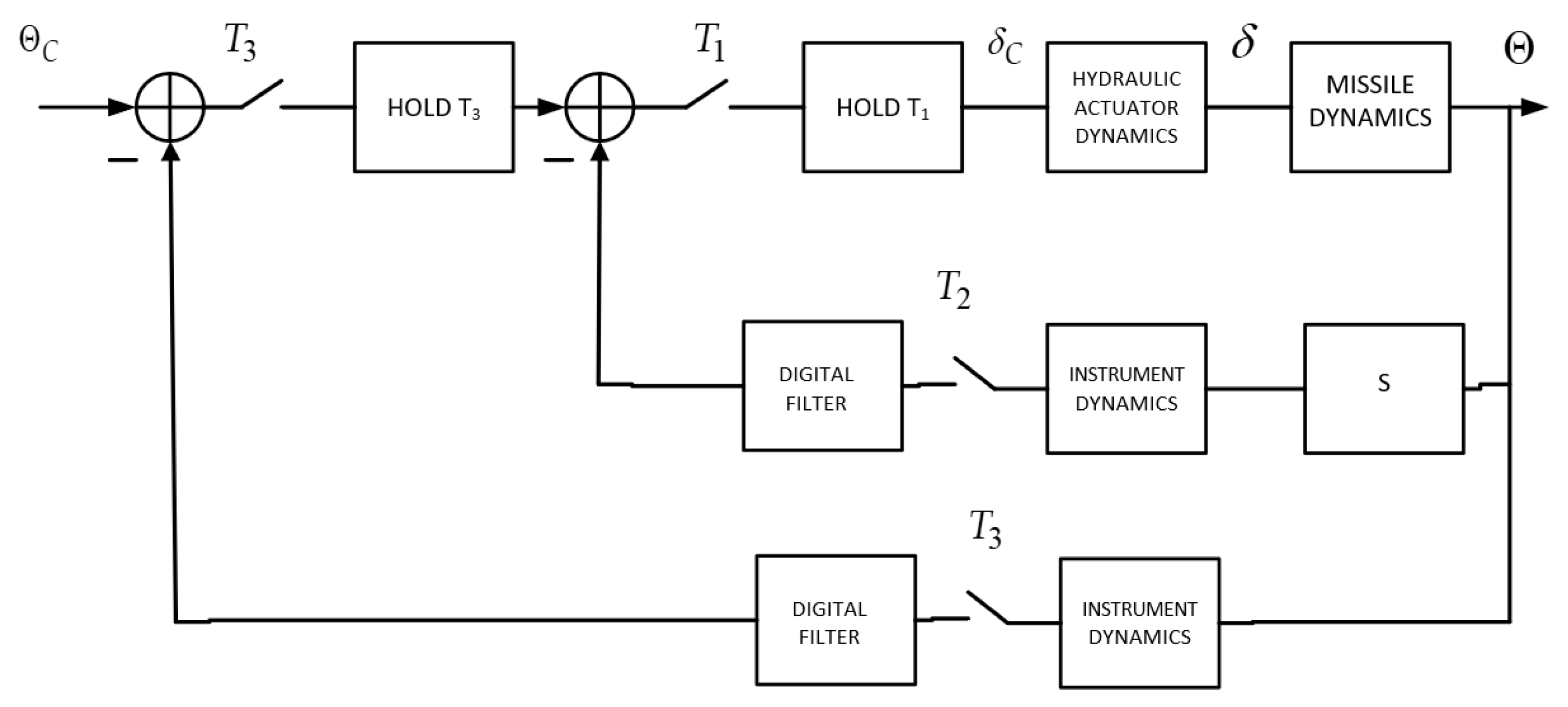
We consider the stabilization system of the lateral movement of the aircraft-type drone when solving the problem of a UAV landing on a non-aircraft-carrying ship [17]. The stabilization system of the lateral movement for the autonomous drone, with an onboard computer in the control loop, is considered in [18], in the form of a structural diagram (Figure 2). The system in Figure 2 is a multiloop multirate continuous-discrete system.

In this figure, $\psi$—yaw angle, $\gamma$—roll angle, ${\delta }_N$, and ${\delta }_E$—angles of deflection of the rudders and ailerons, respectively; ${\epsilon }_N$ and ${\epsilon }_E$—stabilization errors. The corresponding transfer functions are: ${\Phi }_{ST}(s)=\frac{W_{PT}(s)}{1+W_{PT}(s)}$—steering track, $W_{KL}(s)=a_{41}\frac{-\frac{b_{16}{s}^2}{{\mu }_2}+\frac{b_{16}{b}_{33}s}{{\mu }_2}+1}{s(\frac{b_{36}s}{{\mu }_2}+1)}$—kinematic link, $W_e(s)$—extrapolator, $W_{GT}(s)=\frac{s}{(T_{GT}^2{s}^2+2{\zeta }_{GT}{T}_{GT}s+1)({\tau }_{GT}s+1)}$—gyrotachometer, $b_{ij}$—aerodynamic coefficients, $W_{PT}(s)=k_{PT}{W}_{PM}(s)W_{\mu y}(s)$, $W_{PM}(s)=\frac{e^{-{\tau }_{PM}s}}{s(T_{PM}s+1)}$, $W_{\mu y}(s)=\frac{1}{T_{\mu y}s+1}$, $T$ and $\tau$ with the corresponding indices–time constants. The transfer functions of the control object $W_{{\delta }_N\psi }(s)=\frac{\psi (s)}{{\delta }_N(s)}$, $W_{{\delta }_N\gamma }(s)=\frac{\gamma (s)}{{\delta }_N(s)}$, $W_{{\delta }_E\gamma }(s)=\frac{\gamma (s)}{{\delta }_E(s)}$, $W_{{\delta }_E\psi }(s)=\frac{\psi (s)}{{\delta }_E(s)}$ can be determined by transforming, using the Laplace transform for a system of differential equations, describing the rotational motion of the aircraft around the center of mass in the horizontal plane [18]. The transfer function $W_{\psi {\delta }_H}^y(s)$, which characterizes the effect on the dynamics of stabilization of elastic vibrations of a moving UAV, is not taken into account in further consideration. The model of the $W_{\psi {\delta }_H}^y(s)$ is given in [18]. $T_1,\hspace{0.17em}{T}_2,\hspace{0.17em}{T}_3$ are the sampling periods of digital feedback circuits of control signals.

To solve the problem of analysis or synthesis of the system shown in Figure 2, we need to obtain an adequate mathematical model.

The mathematical models obtained using the discrete Laplace transform or z-transform are considered with sufficient simplification. The studies were limited to SISO systems and generally resulted in very cumbersome formulas [1].

Although the problems of analyzing and synthesizing multirate systems appeared a long time ago, there is no explicit and complete methodology for constructing their equivalent mathematical model [1].

Development in the issue of constructing mathematical models of multi-loop control systems with different sampling periods specified using transfer functions was achieved, thanks to the works in references [19,20,21,22]. In these works, it was proposed to replace the pulse elements (keys), which sample signals with different sampling periods, with an equivalent system containing one key and some delay elements. Such an equivalent system operates with a uniform time sampling period. Further description of the considered system is carried out using modified z-transformations, which makes it possible to introduce the time delays of the equivalent system into the description [21]. A description of multiloop multirate systems, in the form of transfer functions and two different algorithms for calculating the characteristic polynomial, was proposed in [19,21]. These two methods, for constructing the characteristic polynomial of a multiloop multirate control system, are equivalent [13].

The main disadvantage of the approach proposed in [19] is the complexity of the implementation associated with the inconvenience of numerical calculations of topological operations [13].

As in most other works, attention in [13] was paid to the construction of characteristic equations of multiloop discrete control systems, containing impulse elements with different sampling periods, and not to the construction of the entire mathematical model of the system suitable for analysis and synthesis.

Thus, existing approaches to the construction of the models of multiloop multirate continuous-discrete systems, in the form of transfer functions, allow one to obtain equations suitable only for studying stability. The existing approaches do not allow a wide range of analysis and synthesis of the specified class of control systems and reduce the efficiency of their research.

Note that the problem of synthesis and analysis of linear continuous-discrete multiloop UAV stabilization systems contains two essential aspects of complexity: the system’s multidimensionality and the multirate of sampling chains. In the case of commensurate periods (their multiplicity to a certain “effective” period), the second aspect is equivalent to the first, significantly strengthening it at large numbers of the multiplicity of sampling periods to the “effective” sampling period. In this case (rationally commensurate sampling periods), it is possible to transform the mathematical model of a multirate system to an equivalent mathematical model of a single-rate system of increased dimension. In the theory of impulse systems, such transformations are usually performed based on the “parallelization” of impulse circuits [1].

In this article, we propose a complete description of a general approach to the construction of an equivalent single-rate model, which makes it possible to transform the vector–matrix model of the original MIMO multiloop multirate system into a vector–matrix model of a single-rate system, in the form typical for vector–matrix models of continuous systems. The construction includes complete descriptions of the equivalent T-single-rate and NT-single-rate, where T is the largest common divisor of the sampling periods of the system, and N is a natural number that is the least common multiple of the numbers characterizing the sampling periods of the system. Detailed descriptions of these characteristics are given below, describing the central element of the construction—a structural invariant of sampling chains—a matrix, which, in the general case, describes a complex situation of the mutual influence of sampling processes in digital circuits of a closed-loop MIMO multirate stabilization system with different sampling periods. The dimension and complexity of this matrix are due to the mutual numerical characteristics of digital circuits.

2. The Mathematical Model of the Stabilization System

To build an equivalent mathematical model of the multirate system, we write the fundamental equation in the input–output form of the Laplace transform. The complete construction of the basic mathematical model in the input–output form of the Laplace transform for the MIMO multiloop multirate continuous-discrete system is given in [18,23].

The continuous object equation and analog circuit stabilization system equation from the object to the sampling keys are

$$\begin{array}{l}y(s)=W_0(s)u(s),\\ x(s)=E(s)y(s)+B(s)u(s),\end{array}$$

(1)

where $W_0(s),\hspace{0.17em}\hspace{0.17em}E(s),\hspace{0.17em}\hspace{0.17em}B(s)$ are the matrices of transfer functions. Usually, $B(s)=0$, and in the future, we will take this into account.

$x(s)={[x_1(s),\hspace{0.17em}{x}_2(s),\dots ,x_r(s)]}^T$ is a vector of the sampling variables with periods $T_1=n_{1}T,\hspace{0.17em}\hspace{0.17em}{T}_2=n_{2}T,\hspace{0.17em}\hspace{0.17em}\dots ,\hspace{0.17em}{T}_r=n_{r}T$, respectively (among which there may be equal ones), where $n_1,\hspace{0.17em}{n}_2,\hspace{0.17em}\dots ,\hspace{0.17em}{n}_r$ are natural numbers. The control vector is a vector $u(s)$. $y(s)$—the vector of outputs.

For the system shown in Figure 2, $x(s)={[x_1(s),\hspace{0.17em}{x}_2(s),x_3(s),x_4(s),x_5(s),x_6(s)]}^T$. For the variables of the vector $x(s)$, the sequence of sampling periods is $T_1,\hspace{0.17em}\hspace{0.17em}{T}_3,\hspace{0.17em}{T}_1,\hspace{0.17em}{T}_3,\hspace{0.17em}{T}_3,\hspace{0.17em}{T}_2$. The vector of outputs $y(s)=\left[\begin{array}{c}\psi \\ \gamma \end{array}\right]$. The “k-th” component of the vector of control, $u_k(s)=-{\displaystyle \sum _{i=1}^r{d}_{ki}(s)x_{i{T}_i}^{*}(s)+u_{Zk}(s)}$, where $d_{ki}(s)$—the transfer function of parallel digital circuits, $x_{1T_1}^{*}(s),\hspace{0.17em}\hspace{0.17em}\hspace{0.17em}{x}_{2T_2}^{*}(s),\hspace{0.17em}\dots ,\hspace{0.17em}{x}_{r{T}_r}^{*}(s)$—discrete Laplace transforms sampled concerning the sampling periods $T_1,\hspace{0.17em}{T}_2,\dots ,T_r$ of the variables $x_1(t),\hspace{0.17em}\hspace{0.17em}{x}_2(t),\hspace{0.17em}\dots ,\hspace{0.17em}{x}_r(t)$, respectively.

As considered in Figure 2, schemes $u_{Z1}(s)={\psi }_Z$, $u_{Z2}(s)={\gamma }_Z$, and the transfer matrixes, $E(s)={\left[\begin{array}{cccccc}0& 0& W_{GT}& 1& s(W_{kZ}+b_{73})& W_{kL}(K_Z(1+K_{Z}s)\\ W_{GT}& 1& 0& 0& 0& 0\end{array}\right]}^T$, $W_0=\left[\begin{array}{cc}{\Phi }_{ST}{W}_{{\delta }_N\psi }& {\Phi }_{ST}{W}_{{\delta }_E\psi }\\ {\Phi }_{ST}{W}_{{\delta }_N\gamma }& {\Phi }_{ST}{W}_{{\delta }_E\gamma }\end{array}\right]$.

Thus

$$x(s)=U(s)u(s)=E(s)W_0(s)u(s).$$

(2)

Writing the equations for the control in a vector–matrix form:

$$u(s)=-W_e(s)W_{*}(s)x_{*}(s)+W_e(s)v^{*}(s),$$

where $W_{*}(s)$ is a matrix with elements $W_{ki{T}_i}^{*}(s)$ and vectors $x_{*}(s),\hspace{0.17em}\hspace{0.17em}\hspace{0.17em}{v}^{*}(s)$ with elements $x_{i{T}_i}^{*}(s)$ and $u_{kzT}^{*}(s)$. The symbol “*” at the bottom marks the property of periodicity of the matrix $W_{*}(s)$ and the vector $x_{*}(s)$ for the corresponding periods. All elements of $W_{*}(s)$ and $x_{*}(s)$ satisfy the relation $x(s+2\pi j/T)=x(s)$. For $W_{*}(s)$ and $x_{*}(s)$ is fulfilled [24,25]

$${(c{b}_{*})}_T^{*}=c_T^{*}{b}_{*}, (\mathrm{or} {(b_{*}c)}_T^{*}{b}_{*}{c}_T^{*}).$$

(3)

Finally, we obtain a mathematical model of the MIMO multiloop multirate continuous-discrete drone stabilization system, which takes into account both the influence of all sampling periods of the system and its multiloop, including the cross-connections of control channels

$$u(s)=-G(s)W_{*}(s)x_{*}(s)+G(s)v^{*}(s),$$

(4)

$$x(s)=-C(s)W_{*}(s)x_{*}(s)+C(s)v^{*}(s),$$

(5)

$$y(s)=-L(s)W_{*}(s)x_{*}(s)+L(s)v^{*}(s),$$

(6)

where $G(s)=W_e(s)I,$ $C(s)=U(s)G(s),$ $L(s)=W_0(s)G(s)$.

Due to the presence in the description of factors that take into account the different sampling periods, the presented mathematical model is not suitable for solving problems of analysis and synthesis. It is a basic model for constructing an equivalent mathematical model, which, in turn, can be used to extend analysis and synthesis methods for multidimensional single-rate systems to the class of multirate systems.

3. Results

As noted earlier, for a fundamental possible transfer of the synthesis and analysis methods of MIMO continuous and discrete systems, to the class of continuous-discrete multirate drone stabilization systems, it is necessary to construct equivalent mathematical models of a single-rate system in a form characteristic for vector–matrix models of continuous systems. Approaches to the construction of equivalent mathematical models are briefly presented in [23]. Now, we give their full description.

3.1. The Equivalent T-Single-Rate Model of the Stabilization System

The given model of a multirate drone stabilization system can be transformed into a model of a single-rate system with a sampling period $T$, which is the greatest common divisor of the sampling periods $T_1,\hspace{0.17em}{T}_2,\dots T_r$.

We will proceed from Equation (11)

$$y_{nT}^{*}(s)=\frac{1}{n}{\displaystyle \sum _{k=1}^n{y}_T^{*}(s+\frac{2\pi j}{nT}(k-1))}, {(x{y}_{nT}^{*})}_T^{*}=x_T^{*}{y}_{nT}^{*}.$$

(7)

Further, until the final results, the symbol $T$ in the designation of the corresponding impulse transformation will be omitted, i.e., for any function $z(s)$, instead of $z_T^{*}(s)$ we will write $z^{*}(s)$.

Consider Equation (4). By property (3), we have

$$x^{*}(s)=-C^{*}(s)W_{*}(s)x_{*}(s)+C^{*}(s)v^{*}(s).$$

(8)

Replacing $s$ in this relation by $s+\frac{2\pi j}{NT}(\nu -1)$, where $N$, $\nu$ are natural numbers, we have

$$x^{*\nu }(s)=-C^{*\nu }(s)W_{*}^{\nu }(s)x_{*}^{\nu }(s)+C^{*\nu }(s)v^{*\nu }(s),$$

(9)

where for any function $\phi (s)$, we further take ${\phi }^{\nu }(s)=\phi (s+\frac{2\pi j}{NT}(\nu -1))$.

Setting in Equation (9), $\nu =1,\dots ,N$, we write

$${\widehat{x}}^{*}(s)=-{\widehat{C}}^{*}(s){\widehat{W}}_{*}(s){\widehat{x}}_{*}(s)+{\widehat{C}}^{*}(s){\widehat{v}}^{*}(s),$$

(10)

where

$$\begin{gathered} \widehat{x}(s)={[x^1(s)\hspace{0.17em}\hspace{0.17em}\hspace{0.17em}{x}^2(s)\hspace{0.17em}\dots \hspace{0.17em}{x}^N(s)]}^T,{\widehat{x}}_{*}(s)={[x_{*}^1(s)\hspace{0.17em}\hspace{0.17em}{x}_{*}^2(s)\hspace{0.17em}\hspace{0.17em}\dots \hspace{0.17em}\hspace{0.17em}{x}_{*}^N(s)]}^T, \\ \widehat{v}(s)={[v^1(s)\hspace{0.17em}\hspace{0.17em}{v}^2(s)\hspace{0.17em}\hspace{0.17em}\hspace{0.17em}\dots \hspace{0.17em}\hspace{0.17em}\hspace{0.17em}{v}^N(s)]}^T, \widehat{C}(s)=diag[C^1(s),\hspace{0.17em}{C}^2(s),\dots ,C^N(s)], \\ \widehat{W}(s)=diag[W^1(s),\hspace{0.17em}{W}^2(s),\dots ,W^N(s)]. \end{gathered}$$

(11)

Consider the components of the vector $x_{*}^{\nu }(s)$

$$x_{i{T}_i}^{\ast \nu }(s)=\frac{1}{n_i}{\displaystyle \sum _{k=1}^{n_i}{x}_i^{\ast }(s+\frac{2\pi j}{NT}(\nu -1)+\frac{2\pi j}{n_{i}T}(k-1))}.$$

(12)

$N$—the least common multiple of numbers $n_1,\hspace{0.17em}{n}_2,\hspace{0.17em}\dots ,\hspace{0.17em}{n}_r$ such that $N={\nu }_1{n}_1,\hspace{0.17em}\hspace{0.17em}\hspace{0.17em}N={\nu }_2{n}_2,\hspace{0.17em}\dots ,\hspace{0.17em}N={\nu }_r{n}_r$, where ${\nu }_1,\hspace{0.17em}{\nu }_2,\dots ,\hspace{0.17em}{\nu }_r$ are natural numbers. Then Equation (12) can be written in the form

$$x_{i{T}_i}^{\ast \nu }(s)=\frac{1}{n_i}{\displaystyle \sum _{k=1}^{n_i}{x}_i^{\ast }(s+\frac{2\pi j}{NT}[\nu +{\nu }_i(k-1)-1])},\hspace{0.17em}\hspace{0.17em}\hspace{0.17em}i=1,\dots ,r.$$

(13)

Note that, for any $p>N$ we have, setting $p=N+\nu$,

$$x_i^{*}(s+\frac{2\pi j}{NT}p)=x_i^{*}(s+\frac{2\pi j}{NT}\nu )$$

(14)

due to the periodicity of the function $x_i^{*}(s)$ in $s$ with a period $2\pi j/T$.

Due to (14), the right-hand side of (13) contains only values $x_i^{*\nu }(s),\hspace{0.17em}\hspace{0.17em}\hspace{0.17em}\nu \in \overline{1,\hspace{0.17em}N},$ which means that there is a linear transformation of the vector ${\widehat{x}}^{*}(s)$ to ${\widehat{x}}_{*}(s)$. We can write

$${\widehat{x}}_{*}(s)=\Pi {\widehat{x}}^{*}(s)$$

(15)

where $\Pi -rN\times rN$ a numerical matrix, the rules for finding, which we indicate below.

Substituting Equation (15) into (10), we find

$${\widehat{x}}^{*}(s)={(I_{rN}+{\widehat{C}}^{*}(s){\widehat{W}}_{*}(s)\prod )}^{-1}{\widehat{C}}^{*}(s){\widehat{v}}^{*}(s).$$

(16)

Writing the equation

$$\widehat{y}(s)=-\widehat{L}(s){\widehat{W}}_{*}(s){\widehat{x}}_{*}(s)+\widehat{L}(s){\widehat{v}}^{*}(s),$$

where $\widehat{y}(s)={[y^1(s)\hspace{0.17em}{y}^2(s)\dots \hspace{0.17em}{y}^N(s)]}^T$, $\widehat{L}(s)=diag[L^1(s),\hspace{0.17em}{L}^2(s),\dots ,\hspace{0.17em}{L}^N(s)]\hspace{0.17em}$, and using (15), (16) we find

$$\widehat{y}(s)=\widehat{L}(s)\{-{\widehat{W}}_{*}(s)\prod {(I_{rN}+{\widehat{C}}^{*}(s){\widehat{W}}_{*}(s)\prod )}^{-1}{\widehat{C}}^{*}(s)+I_{mN}\}{\widehat{v}}^{*}(s).$$

(17)

Applying the identity [26,27,28] ${I-\mathrm{A}(I+\mathrm{BA})}^{-1}{\mathrm{B}=(I+\mathrm{AB})}^{-1}$, we also find

$$\begin{gathered} \widehat{y}(s)=\widehat{L}(s){(I_{mN}+{\widehat{W}}_{*}(s)\prod {\widehat{C}}^{*}(s))}^{-1}{\widehat{v}}^{*}(s), \\ {\widehat{y}}^{*}(s)={\widehat{L}}^{*}(s){(I_{mN}+{\widehat{W}}_{*}(s)\prod {\widehat{C}}^{*}(s))}^{-1}{\widehat{v}}^{*}(s). \end{gathered}$$

(18)

The defining matrix $\Pi =\left\{{\Pi }_{\nu p}\right\},\hspace{0.17em}\hspace{0.17em}\nu ,p\in \overline{1,\hspace{0.17em}N}$ as block type, where ${\Pi }_{\nu p}\hspace{0.17em}-\hspace{0.17em}r\times r$ matrix, and introducing the notation

$$W^{*}(s)={\widehat{W}}_{*}(s)\prod {\widehat{C}}^{*}(s)$$

(19)

we define the elements of the block representation of this matrix

$$W^{*}(s)=\{W_{\nu p}^{*}(s)\},\hspace{0.17em}\nu ,p\in \overline{1,\hspace{0.17em}N}, W_{\nu p}^{*}(s)=W_{*}^{\nu }(s){\prod }_{\nu p}{C}^{*p}(s),\hspace{0.17em}\nu ,p\in \overline{1,\hspace{0.17em}N}.$$

(20)

where ${\prod }_{\nu p}=diag[{\pi }_{\nu p}^1,\hspace{0.17em}{\pi }_{\nu p}^2,\dots ,\hspace{0.17em}{\pi }_{\nu p}^r]$.

From (20). we obtain the equation for the elements of the matrix $W_{\nu p}^{*}(s)$

$$W_{\nu p}^{\ast \sigma \mu }(s)={\displaystyle \sum _{i=1}^r{\pi }_{\nu p}^i{W}_{\ast \sigma i}(s+(\nu -1)\frac{2\pi j}{NT})C_{i\mu }^{\ast }(s+(p-1)\frac{2\pi j}{NT})}.$$

(21)

The construction of the matrix (20) of an equivalent T-single-rate system allows one to find the outputs of the closed original system, sampled at the moments $kT,\hspace{0.17em}\hspace{0.17em}\hspace{0.17em}k=0,\hspace{0.17em}1,\hspace{0.17em}\dots$.

Defining, for this purpose, the block type matrix

$$H^{*}{\left(s\right)=(I}_{\mathrm{mN}}{+W}^{*}{\left(s\right))}^{-1}, H^{*}{=\{H}_{\nu p}^{*}\}, \nu ,\hspace{0.17em}p\in \overline{1, N},$$

we find

$$y^{*}(s)={\displaystyle \sum _{p=1}^N{L}^{*}(s)H_{1p}^{*}(s)u^{*p}(s)},$$

(22)

where $y^{*}(s)=y^{*1}(s),$ $L^{*}(s)=L^{*1}(s)$.

3.2. The Equivalent T-Single-Rate Model of the Stabilization System: The Analog Control

In order to not change the notation of the matrices, we assume that $v(s)$ is a vector with elements $\frac{1}{W_e(s)}{u}_{kz}(s),\hspace{0.17em}\hspace{0.17em}\hspace{0.17em}k=1,\hspace{0.17em}\dots ,r$.

Instead of (4)–(6), we now consider the equations

$$u(s)=-G(s)W_{*}(s)x_{*}(s)+G(s)v(s),$$

$$x(s)=-C(s)W_{*}(s)x_{*}(s)+C(s)v(s),$$

$$y(s)=-L(s)W_{*}(s)x_{*}(s)+L(s)v(s).$$

Determining, as above, the extended vectors and matrices (14), we find

$${\widehat{x}}^{*}(s)=-{\widehat{C}}^{*}(s){\widehat{W}}_{*}(s){\widehat{x}}_{*}(s)+{[\widehat{C}(s)\widehat{v}(s)]}^{*},$$

$${\widehat{x}}^{*}(s)={(I_{rN}+{\widehat{C}}^{*}(s){\widehat{W}}_{*}(s)\Pi )}^{-1}{[\widehat{C}(s)\widehat{v}(s)]}^{*},$$

$${\widehat{y}}^{*}(s)=-{\widehat{L}}^{*}(s){\widehat{W}}_{*}(s)\Pi {(I_{rN}+{\widehat{C}}^{*}(s){\widehat{W}}_{*}(s)\Pi )}^{-1}{[\widehat{C}(s)\widehat{v}(s)]}^{*}+{[\widehat{L}(s)\widehat{v}(s)]}^{*},$$

(23)

Hence, what follows is the corresponding representation for the impulse transformation of the vector of outputs, similar to Equation (22).

3.3. The Equivalent NT-Single-Rate Model of the Stabilization System

The construction of the sequence $y(kT),\hspace{0.17em}\hspace{0.17em}\hspace{0.17em}k=0,1,\hspace{0.17em}\dots$ allows, of course, to isolate the sequence $y(kNT),\hspace{0.17em}\hspace{0.17em}\hspace{0.17em}k=0,1,\hspace{0.17em}\dots$. At the same time, if the last sequence is determined from the discrete Laplace transformation $y_{NT}^{*}(s)$, then this one can see some additional possibilities of analyzing the dynamics of the initial multirate stabilization system. Therefore, it is of interest to consider $NT$—a single-rate equivalent model—an impulse stabilization system with a sampling period $NT$, where, as before, $N$ is the least common multiple of numbers $n_1,\hspace{0.17em}\dots ,\hspace{0.17em}{n}_r$$(N={\nu }_1{n}_1,\hspace{0.17em}N={\nu }_2{n}_2,\hspace{0.17em}\dots ,\hspace{0.17em}N={\nu }_r{n}_r)$.

The starting point for building an $NT$—single-rate equivalent model is the [29]

$$y_T^{*}(s)={\displaystyle \sum _{k=1}^n{e}^{-(k-1)Ts}{[y(s)e^{(k-1)Ts}]}_{nT}^{*}}.$$

(24)

Taking into account $T_i=NT/{\nu }_i,\hspace{0.17em}\hspace{0.17em}i=1,\hspace{0.17em}\hspace{0.17em}\dots ,\hspace{0.17em}r$,

$$x_{i{T}_i}^{*}(s)={\displaystyle \sum _{\nu =1}^{{\nu }_i}{e}^{-(\nu -1)T_{i}s}{[x_i(s)e^{(\nu -1)T_{i}s}]}_{NT}^{*}={\displaystyle \sum _{\nu =1}^{{\nu }_i}{e}_{\nu i}^{-}{[x_i(s)e_{\nu i}^{+}]}_{NT}^{*}}},$$

(25)

where the numbers $e_{\nu i}^{\pm }=e^{\pm (\nu -1)T_{i}s},\hspace{0.17em}\hspace{0.17em}\hspace{0.17em}\nu =1,\hspace{0.17em}\dots ,\hspace{0.17em}{\nu }_i;\hspace{0.17em}\hspace{0.17em}i=1,\hspace{0.17em}\dots ,\hspace{0.17em}r$.

Equation (25) can be written as

$$x_{i{T}_i}^{*}(s)={\displaystyle \sum _{\nu =1}^{N_i}{e}_{\nu i}^{-}{x}_{\nu iNT}^{*}(s)=E_i^{-}(s){\widehat{x}}_{iNT}^{*}(s)},$$

(26)

where $E_i^{-}(s)=[e_{1i}^{-},\hspace{0.17em}\hspace{0.17em}{e}_{2i}^{-},\hspace{0.17em}\dots \hspace{0.17em},\hspace{0.17em}{e}_{{\nu }_{i}i}^{-}]$, ${\widehat{x}}_i(s)={[x_{1i}(s)\hspace{0.17em}\hspace{0.17em}{x}_{2i}(s)\dots x_{{\nu }_{i}i}(s)]}^T,\hspace{0.17em}\hspace{0.17em}\hspace{0.17em}\hspace{0.17em}i=1,\hspace{0.17em}\dots ,\hspace{0.17em}r$, $x_{\nu i}(s)=e_{\nu i}^{+}{x}_i(s)$.

Using Equation (25) and the block matrix $E(s)=diag[E_1^{-}(s)\hspace{0.17em}\hspace{0.17em}\hspace{0.17em}{E}_2^{-}(s)\hspace{0.17em}\hspace{0.17em}\hspace{0.17em}\dots \hspace{0.17em}\hspace{0.17em}\hspace{0.17em}{E}_r^{-}(s)]\hspace{0.17em}$ with dimension $r\times ({\nu }_1+{\nu }_2+\cdots +{\nu }_r)$ for a vector $x_{*}(s)={[x_{1T_1}^{*}(s)\hspace{0.17em}\hspace{0.17em}\hspace{0.17em}\hspace{0.17em}{x}_{2T_2}^{*}(s)\dots \hspace{0.17em}\hspace{0.17em}\hspace{0.17em}\hspace{0.17em}{x}_{r{T}_r}^{*}(s)]}^T$, we can write $x_{*}(s)=E^{-}(s){\widehat{x}}_{NT}^{*}(s)$ and

$$x(s)=-C(s)W_{*}(s)E^{-}(s){\widehat{x}}_{NT}^{*}(s)+C(s)v^{*}(s),$$

(27)

We now introduce the matrix $E_i^{+}(s)={[e_{1i}^{+}(s)\hspace{0.17em}\hspace{0.17em}\hspace{0.17em}{e}_{2i}^{+}(s)\dots \hspace{0.17em}\hspace{0.17em}\hspace{0.17em}{e}_{{\nu }_{i}i}^{+}(s)]}^T$ and block matrix $E(s)=diag[E_1^{+}(s),\hspace{0.17em}\hspace{0.17em}\hspace{0.17em}{E}_2^{+}(s),\hspace{0.17em}\hspace{0.17em}\dots ,\hspace{0.17em}\hspace{0.17em}\hspace{0.17em}{E}_r^{+}(s)\hspace{0.17em}]$ with a dimension $({\nu }_1+{\nu }_2+\cdots +{\nu }_r)\times r$ that allows writing $E^{+}(s)x(s)=\widehat{x}(s)$.

Therefore, multiplying (27) on the left by the matrix $E^{+}(s)$, we obtain

$$\widehat{x}(s)=-E^{+}(s)C(s)W_{*}(s)E^{-}(s){\widehat{x}}_{NT}^{*}(s)+E^{+}(s)C(s)v^{*}(s).$$

(28)

Introducing, for convenience, $C^{+}(s)=E^{+}(s)C(s)$, $W_{*}^{-}(s)=W_{*}(s)E^{-}(s)$ and $W_{NT}^{*}(s)={[C^{+}(s)W_{*}^{-}(s)]}_{NT}^{*}$, by Equation (28), we find

$${\widehat{x}}_{NT}^{*}(s)={[I_{\sigma }+W_{NT}^{*}(s)]}^{-1}{[C^{+}(s)v^{*}(s)]}_{NT}^{*},$$

(29)

where $\sigma ={\nu }_1+{\nu }_2+\cdots +{\nu }_r$.

We also find

$$y_{NT}^{*}(s)=-{[L(s)W_{*}^{-}(s)]}_{NT}^{*}{[I_{\sigma }+W_{NT}^{*}(s)]}^{-1}{[C^{+}(s)v^{*}(s)]}_{NT}^{*}+{[L(s)v^{*}(s)]}_{NT}^{*}.$$

(30)

The relations (29) and (30) define the equivalent single-rate model of the closed-loop drone stabilization system with a sampling period $NT$.

An alternative approach to constructing an equivalent single-rate model of the closed-loop drone stabilization system with a sampling period $NT$ is given in [28].

3.4. The Structural Invariant of Sampling Chains of the Stabilization System

3.4.1. The Construction Method of the Structural Invariant of Sampling Chains of the Stabilization System

When, in stabilization system (4)–(6), the same sampling period is T, then $n_1=n_2=\dots =n_r=1$ and $N=1$. The block vectors and matrices introduced above degenerate (consist of one block element). Equation (18) takes the form

$$y^{*}(s)=L^{*}(s){(I_m+W^{*}(s)C^{*}(s))}^{-1}{v}^{*}(s).$$

(31)

Here, the matrix $\Pi =I_r$ degenerates into one block with diagonal elements equal to one.

In the general case of modeling multidimensional multiloop multirate stabilization systems, there is a complex situation of the mutual influence of sampling processes in digital circuits of a closed system with different sampling periods. A characteristic element of the description of this complex situation is the matrix $\Pi$, i.e., transformation (15).

The dimension and complexity of this matrix determine the dimension and complexity of the processes in the stabilization system, and is due to the mutual numerical characteristics of the digital circuits—the numbers $n_1,\dots ,n_r$ that determine the relationship between the sampling periods and $N$—is the least common multiple of the indicated numbers.

As can be seen from Equations (13) and (15), only numbers $\frac{1}{n_i},\hspace{0.17em}i=1,\dots ,r$ are nonzero entries of this matrix. Since these numbers have the meaning of relative sampling period densities (ratios of the number of “rare” samples to the number of “frequent” ones), the matrix $\Pi$ will be called the matrix of tilt densities. Since the structure of the system, in particular, the arrangement of digital chains and sampling keys, does not affect the matrix $\Pi$ in any way, it is a structural invariant of the sampling chains.

To complete the formation of an equivalent single-rate model of the stabilization system, we now indicate a method for calculating the elements of the matrix $\Pi$. We will look for them in the form of the matrix ${\prod }_{\nu p}=diag[{\pi }_{\nu p}^1,\hspace{0.17em}{\pi }_{\nu p}^2,\dots ,\hspace{0.17em}{\pi }_{\nu p}^r]$. To do this, consider the equation

$${\displaystyle \sum _{p=1}^N{\pi }_{\nu p}^i{x}_i^{*p}=\frac{1}{n_i}}{\displaystyle \sum _{k=1}^{n_i}{x}_i^{*\nu +(k-1){\nu }_i}},$$

(32)

which takes place by Equations (13) and (15) with the notation

$$x_i^{*p}(s)=x_i^{*}(s+(p-1)\frac{2\pi j}{NT}),\hspace{0.17em}i=1,\dots ,r.$$

Considering Equation (32), one should take into account the periodicity relation

$$x_i^{*N+p}=x_i^{*p},\hspace{0.17em}p=1,2,\dots ,$$

as property (14) of functions $x_i^{*}(s),\hspace{0.17em}i=1,\dots ,r$.

For this purpose, consider the right-hand side of relation (32) and the set of numbers

$$p(k)=\nu +(k-1){\nu }_i,\hspace{0.17em}k=1,\dots ,\hspace{0.17em}{n}_i,$$

(33)

with fixed indices $\nu ,\hspace{0.17em}i$.

The numbers of this set have the property

$$p(k^{″})>p(k^{\prime }),\hspace{0.17em}{k}^{″}>k^{\prime }.$$

$p_{\max }$ be the largest of the numbers $p(k,\hspace{0.17em}\nu ,\hspace{0.17em}i)=\nu +(k-1){\nu }_i$, $k\in \overline{1,\hspace{0.17em}{n}_i};\hspace{0.17em}\nu \in \overline{1,\hspace{0.17em}N};\hspace{0.17em}i\in \overline{1,\hspace{0.17em}r}$. This number has the form

$$p_{\max }=\underset{i\in \overline{1,r}}{\max }(N+(n_i-1){\nu }_i)=N+N-\overline{\nu }=N+\overline{\gamma }.$$

where $\overline{\nu }$ is the smallest of the numbers ${\nu }_i,\hspace{0.17em}i\in \overline{1,r}$.

Due to the $N=n_i{\nu }_i$, at least one of the numbers ${\nu }_i,\hspace{0.17em}i\in \overline{1,r}$ is less then $N$ (at least one of the numbers $n_i,\hspace{0.17em}i\in \overline{1,r}$ is greater than (1), which means $\overline{\gamma }<N$.

As a result, all numbers of form (33) exceeding $N$ are numbers of the form $N+\gamma ,\hspace{0.17em}0\le \gamma \le N-1$. Now, let, for arbitrarily taken $k^{″},\hspace{0.17em}{k}^{\prime },\hspace{0.17em}k$, such that $k^{″}>k^{\prime }>k$, we have

$$p(k)=\nu +(k-1){\nu }_i=\gamma \le N,$$

$$p(k^{\prime })=\nu +(k^{\prime }-1){\nu }_i=N+{\gamma }^{\prime }$$

$$p(k^{″})=\nu +(k^{″}-1){\nu }_i=N+{\gamma }^{″}$$

Subtracting, we find that

$$\begin{array}{l}{\gamma }^{″}-{\gamma }^{\prime }=(k^{″}-k^{\prime }){\nu }_i,\hspace{0.17em}\\ \gamma -{\gamma }^{\prime }=(k-k^{″}){\nu }_i+N=(n_i+k-k^{″}){\nu }_i.\end{array}$$

Hence,

$${\gamma }^{\prime }<{\gamma }^{″}<\gamma .$$

Because of the above, from (35), we obtain the following rule for calculating the elements ${\pi }_{\nu l}^i,\hspace{0.17em}l=1,\dots ,N$ of the matrix $\Pi$ of quantization densities for fixed indices $\nu ,\hspace{0.17em}i$

$${\pi }_{\nu l}^i=\{\begin{array}{l}1/n_i,\hspace{0.17em}\hspace{0.17em}l=l(k)=p(k),\hspace{0.17em}\hspace{0.17em}\hspace{0.17em}p(k)\le N\\ 1/n_i,\hspace{0.17em}\hspace{0.17em}l=l(k)=p(k)-N,\hspace{0.17em}\hspace{0.17em}p(k)>N\\ 0\hspace{0.17em}\hspace{0.17em}\hspace{0.17em}\hspace{0.17em}\hspace{0.17em}\hspace{0.17em}\hspace{0.17em}l\ne l(k),\end{array}$$

where the values $p(k),\hspace{0.17em}k=1,\dots ,n_i$ are calculated by (33).

3.4.2. The Algorithm of Construction the Structural Invariant of Sampling Chains of the Stabilization System

In this part, we present the corresponding algorithm. We build the table to construct the matrix $\Pi$ (

Table 1. The table to construct the matrix $\Pi$.

p	1	2		*			*		N
$\delta (p)$			…0	1	0	…0	1	0…

).

The top line of the table is a series of natural numbers from 1 to $N$, some of them are marked with an asterisk —*. The second line contains values $\delta (p)$ equal to 1 under the marked upper numbers and 0 otherwise.

The rule for marking the numbers on the top line is as follows. The values are calculated

$$p\left(k\right)=\nu +(k-1){\nu }_i,\hspace{0.17em}k=1,\dots ,n_i.$$

If $p(k)\le N$, then the marked number $p_{*}=p(k)$, if

$$p(k)=N+\gamma (k),$$

then $p_{*}={\gamma }_k$.

In this way, the bottom line defines the values $\delta \left(p\right),\hspace{0.17em}l=1,\dots ,\hspace{0.17em}N$, and

$${\pi }_{\nu p}^i=\frac{1}{n_i}\delta (p),\hspace{0.17em}p=1,\dots ,\hspace{0.17em}N.$$

Thus, this method determines the entire row of the matrix $\Pi$, i.e., diagonal elements with fixed indices $\nu ,\hspace{0.17em}i$ of all block matrices equal to either $\frac{1}{n_i}$ or 0.

Adopting $\nu =1$ and applying the algorithm n times for $i=1,\dots ,\hspace{0.17em}r$, we finally find the first row of the block representation of the density matrix $\Pi$

$${\Pi }_{11},\hspace{0.17em}{\Pi }_{12},\hspace{0.17em}\dots \hspace{0.17em},\hspace{0.17em}{\Pi }_{1N-1},\hspace{0.17em}{\Pi }_{1N}.$$

This row defines the entire matrix $\Pi$ using a sequential circular permutation. For example, the second line will be

$${\Pi }_{1N},\hspace{0.17em}{\Pi }_{11},\hspace{0.17em}\dots ,\hspace{0.17em}{\Pi }_{1N-2},\hspace{0.17em}{\Pi }_{1N-1}, \mathrm{etc}.$$

For example, for $N=3$, the entire matrix has the form

$$\Pi =\Vert \begin{array}{ccc}{\Pi }_{11}& {\Pi }_{12}& {\Pi }_{13}\\ {\Pi }_{13}& {\Pi }_{11}& {\Pi }_{12}\\ {\Pi }_{12}& {\Pi }_{13}& {\Pi }_{11}\end{array}\Vert .$$

Note the possibility of forming the given blocks of the matrix $\Pi$. For example, we are talking about a block ${\Pi }_{\nu p}$. Diagonal elements ${\pi }_{\nu p}^i,\hspace{0.17em}i=1,\dots ,\hspace{0.17em}r$ should be defined with, given $\nu ,\hspace{0.17em}p$. Then:

• If $k\in \overline{1,n_i}$ exists, satisfying one of the equations

  $$\nu +(k-1){\nu }_i=p,\hspace{0.17em}\nu +(k-1){\nu }_i-N=p,$$

  (34)

  then ${\pi }_{\nu p}^i=\frac{1}{n_i}$, and
• If $k\in \overline{1,n_i}$ does not exist, then ${\pi }_{\nu p}^i=0$.

Thus, the construction algorithm is fully formulated.

3.4.3. Example

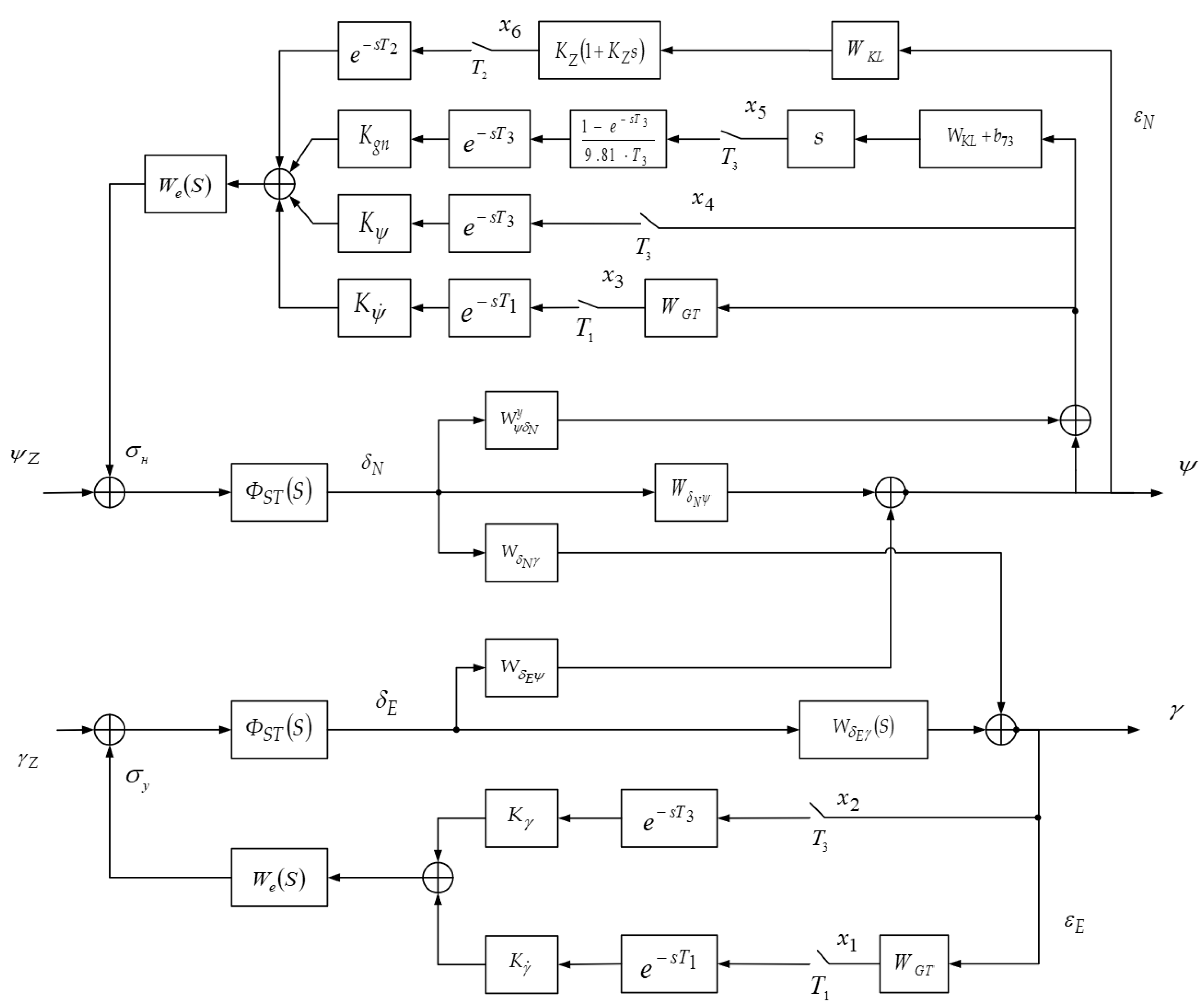
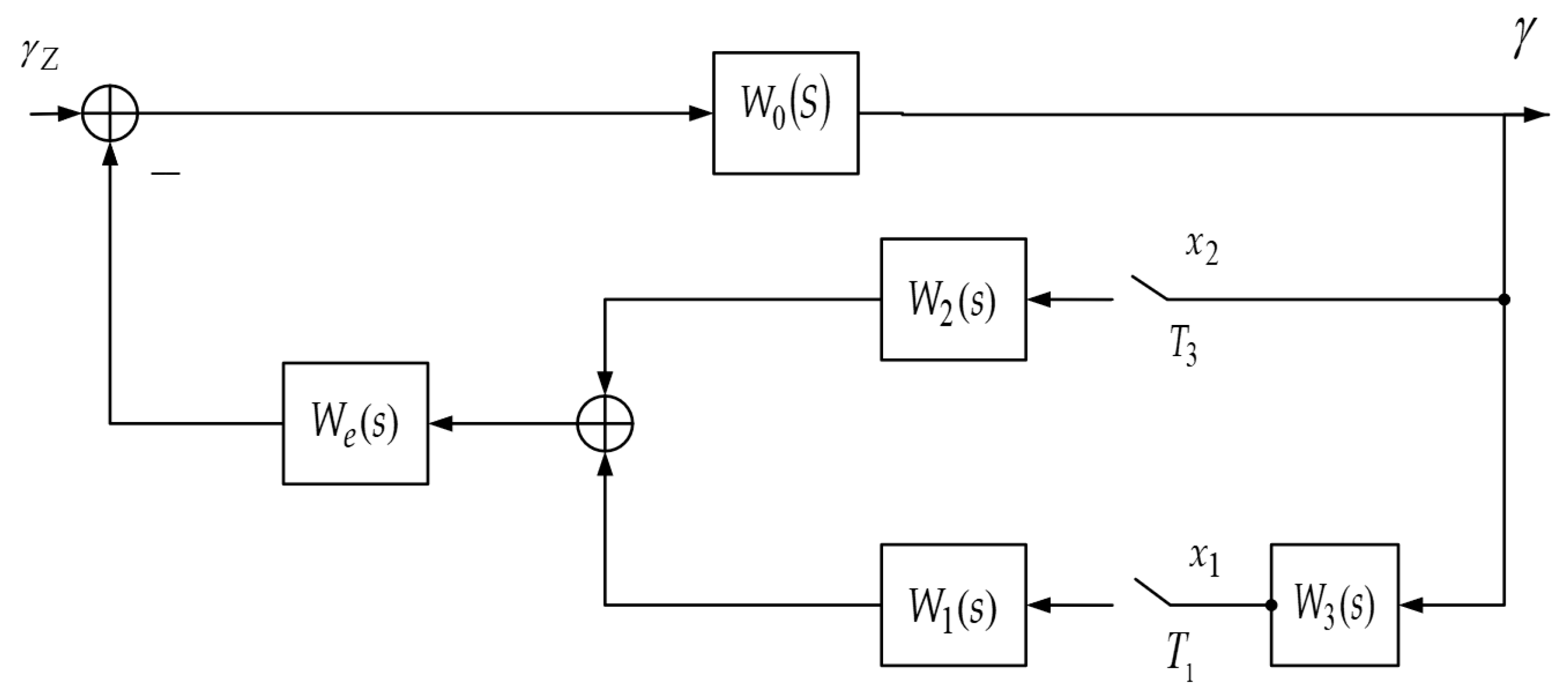
Consider a part of the lateral motion stabilization system—a modified roll stabilization contour (Figure 3).

For the system shown in Figure 3, according to the notation introduced in Section 2, we have: $W_0(s)={\Phi }_{ST}(s)\cdot W_{{\delta }_E\gamma }(s)$, $x(s)={\left[\begin{array}{cc}{x}_1(s)& x_2(s)\end{array}\right]}^T$,$y(s)=\gamma$, $E(s)={\left[W_1(s)\hspace{0.17em}\hspace{0.17em}\hspace{0.17em}{W}_2(s)\right]}^T$, $B(s)=0$, $W_{*}(s)=\left[\begin{array}{cc}{W}_{1T_1}^{*}(s)& W_{2T_3}^{*}(s)\end{array}\right]$, $G(s)=W_e(s)$,$L(s)=W_e(s)W_0(s)$, $C(s)=\left[\begin{array}{c}{W}_e(s)W_3(s)W_0(s)\\ W_e(s)W_0(s)\end{array}\right]$.

From the above diagram, it is clear that the methods based on the analysis of the location of the poles are not available with such a representation of the system.

Using Equations (1)–(6), we obtain an expression for the output of the system

$$y(s)=-W_e(s)W_0(s)[W_{1*}(s)\hspace{0.17em}{W}_{2*}(s)]\left[\begin{array}{l}{x}_{1*}(s)\\ x_{2*}(s)\end{array}\right]+W_e(s)W_0(s)u^{*}(s),$$

(35)

To construct an equivalent model, the usual matrix operations are used. A separate issue is the construction of a matrix of sampling densities.

For the considered in a Figure 3 system $r=2,\hspace{0.17em}{n}_1=1,\hspace{0.17em}{n}_2=3$ (defined above). Using the above equations, we obtain $N=3,\hspace{0.17em}{\nu }_1=3,\hspace{0.17em}{\nu }_2=1$.

For block ${\Pi }_{11}$, we have the equations

$$\begin{array}{l}i=1\hspace{0.17em}\hspace{0.17em}\hspace{0.17em}\hspace{0.17em}\hspace{0.17em}\hspace{0.17em}1+(k-1)3=1,\hspace{0.17em}\hspace{0.17em}\hspace{0.17em}\hspace{0.17em}1+(k-1)3-3=1,\hspace{0.17em}\hspace{0.17em}\hspace{0.17em}k\in \overline{1};\\ i=2\hspace{0.17em}\hspace{0.17em}\hspace{0.17em}\hspace{0.17em}\hspace{0.17em}1+(k-1)1=1,\hspace{0.17em}\hspace{0.17em}\hspace{0.17em}\hspace{0.17em}\hspace{0.17em}1+(k-1)1-3=1,\hspace{0.17em}\hspace{0.17em}\hspace{0.17em}\hspace{0.17em}k\in \overline{1,3}.\end{array}$$

Therefore, ${\pi }_{11}^1=1,\hspace{0.17em}{\pi }_{11}^2=\frac{1}{3}$.

For block ${\Pi }_{12}$:

$$\begin{array}{l}i=1\hspace{0.17em}\hspace{0.17em}\hspace{0.17em}\hspace{0.17em}\hspace{0.17em}\hspace{0.17em}1+(k-1)3=2,\hspace{0.17em}\hspace{0.17em}\hspace{0.17em}\hspace{0.17em}1+(k-1)3-3=2,\hspace{0.17em}\hspace{0.17em}\hspace{0.17em}k\in \overline{1};\\ i=2\hspace{0.17em}\hspace{0.17em}\hspace{0.17em}\hspace{0.17em}\hspace{0.17em}1+(k-1)1=2,\hspace{0.17em}\hspace{0.17em}\hspace{0.17em}\hspace{0.17em}\hspace{0.17em}1+(k-1)1-3=2,\hspace{0.17em}\hspace{0.17em}\hspace{0.17em}\hspace{0.17em}k\in \overline{1,3}.\end{array}$$

Therefore, ${\pi }_{12}^1=0,\hspace{0.17em}{\pi }_{12}^2=\frac{1}{3}$.

For block ${\Pi }_{13}$

$$\begin{array}{l}i=1\hspace{0.17em}\hspace{0.17em}\hspace{0.17em}\hspace{0.17em}\hspace{0.17em}\hspace{0.17em}1+(k-1)3=3,\hspace{0.17em}\hspace{0.17em}\hspace{0.17em}\hspace{0.17em}1+(k-1)3-3=3,\hspace{0.17em}\hspace{0.17em}\hspace{0.17em}k\in \overline{1};\\ i=2\hspace{0.17em}\hspace{0.17em}\hspace{0.17em}\hspace{0.17em}\hspace{0.17em}1+(k-1)1=3,\hspace{0.17em}\hspace{0.17em}\hspace{0.17em}\hspace{0.17em}\hspace{0.17em}1+(k-1)1-3=3,\hspace{0.17em}\hspace{0.17em}\hspace{0.17em}\hspace{0.17em}k\in \overline{1,3}.\end{array}$$

Therefore, ${\pi }_{13}^1=0,\hspace{0.17em}{\pi }_{12}^2=\frac{1}{3}$.

The entire density matrix has the form

$$\Pi =\left[\begin{array}{cccccc}1& 0& 0& 0& 0& 0\\ 0& \frac{1}{3}& 0& \frac{1}{3}& 0& \frac{1}{3}\\ 0& 0& 1& 0& 0& 0\\ 0& \frac{1}{3}& 0& \frac{1}{3}& 0& \frac{1}{3}\\ 0& 0& 0& 0& 0& 0\\ 0& \frac{1}{3}& 0& \frac{1}{3}& 0& \frac{1}{3}\end{array}\right].$$

The difference in the sampling densities is reflected in the matrix $\Pi$ by the inhomogeneous filling of its blocks. When the sampling density in all circuits is the same, i.e., $n_1=n_2=\cdots =n_r=n,\hspace{0.17em}N=n$ and ${\nu }_1={\nu }_2=\cdots ={\nu }_r=1$, then the matrix $\Pi$ turns out to be maximally filled—all of its block elements ${\Pi }_{\nu p},\hspace{0.17em}\nu ,p=1,\dots ,\hspace{0.17em}n$ turn out to be equal

$${\Pi }_{\nu p}=\frac{1}{n}{I}_r.$$

where $I_r$—identity $r\hspace{0.17em}x\hspace{0.17em}r$ matrix. Hence, ${\pi }_{\nu p}^i=\frac{1}{n_i},\hspace{0.17em}i\in \overline{1,r}$.

For the system under consideration, to construct a T—single-rate equivalent model, we will have the following vectors and matrices used to construct the model:

$${\widehat{x}}_{*}(s)=\left[\begin{array}{c}{x}_{*}^1(s)\\ x_{*}^2(s)\\ x_{*}^3(s)\end{array}\right] \mathrm{with} \mathrm{dimension} 3 \times 1; \widehat{v}(s)=\left[\begin{array}{c}{v}^1(s)\\ v^2(s)\\ v^3(s)\end{array}\right] \mathrm{with} \mathrm{dimension} 3 \times 1;$$

$$\widehat{C}(s)=\left[\begin{array}{ccc}{C}^1(s)& & 0\\ & C^2(s)& \\ 0& & C^3(s)\end{array}\right] \mathrm{with} \mathrm{dimension} 6 \times 3,$$

where the dimension of the matrix block $C^i(s)$—2 × 1;

$$\widehat{W}(s)=\left[\begin{array}{ccc}{W}^1(s)& & 0\\ & W^2(s)& \\ 0& & W^3(s)\end{array}\right] \mathrm{with} \mathrm{dimension} 3 \times 6;$$

where the dimension of the matrix block $W^i(s)$—1 × 2;

$$\widehat{L}(s)=\left[\begin{array}{ccc}{L}^1(s)& & 0\\ & L^2(s)& \\ 0& & L^3(s)\end{array}\right] \mathrm{with} \mathrm{dimension} 3 \times 1;$$

$$\widehat{y}(s)=\left[\begin{array}{c}{y}^1(s)\\ y^2(s)\\ y^3(s)\end{array}\right] \mathrm{with} \mathrm{dimension} 3 \times 1$$

.

Knowing the indicated matrices, we get

$${\widehat{y}}^{*}(s)={\widehat{L}}^{*}(s){(I_{mN}+{\widehat{W}}_{*}(s)\prod {\widehat{C}}^{*}(s))}^{-1}{\widehat{v}}^{*}(s),$$

or

$$\begin{array}{l}\left[\begin{array}{c}{y}^{*1}(s)\\ y^{*2}(s)\\ y^{*3}(s)\end{array}\right]=\left[\begin{array}{ccc}{L}^1(s)& 0& 0\\ 0& L^2(s)& 0\\ 0& 0& L^3(s)\end{array}\right]\times \\ \times {\left(\begin{array}{l}\left[\begin{array}{ccc}1& 0& 0\\ 0& 1& 0\\ 0& 0& 1\end{array}\right]+\left[\begin{array}{cccccc}{W}_{1T_1}^{*1}& W_{2T_2}^{*1}& 0& 0& 0& 0\\ 0& 0& W_{1T_1}^{*2}& W_{2T_2}^{*2}& 0& 0\\ 0& 0& 0& 0& W_{1T_1}^{*3}& W_{2T_2}^{*3}\end{array}\right]\left[\begin{array}{cccccc}1& 0& 0& 0& 0& 0\\ 0& \frac{1}{3}& 0& \frac{1}{3}& 0& \frac{1}{3}\\ 0& 0& 1& 0& 0& 0\\ 0& \frac{1}{3}& 0& \frac{1}{3}& 0& \frac{1}{3}\\ 0& 0& 0& 0& 0& 0\\ 0& \frac{1}{3}& 0& \frac{1}{3}& 0& \frac{1}{3}\end{array}\right]\times \\ \times \left[\begin{array}{ccc}{C}_1^{1*}& 0& 0\\ C_2^{1*}& 0& 0\\ 0& C_1^{2*}& 0\\ 0& C_2^{2*}& 0\\ 0& 0& C_1^{3*}\\ 0& 0& C_2^{3*}\end{array}\right]\end{array}\right)}_{}^{-1}\left[\begin{array}{c}{u}_{}^{1*}\\ u_{}^{2*}\\ u_{}^{3*}\end{array}\right].\end{array}$$

By separating $y^{*1}(s)$, we get an equivalent single-rate model as a result. The rest of the equivalent models given in the article are obtained in the same way.

A comparative analysis of the step response of stabilization systems for the different types of models was carried out in [18]: a complete continuous-discrete system, taking into account the presence of different sampling periods, a model of a system in which all quantization periods are considered small, and are excluded from the model, and the model in which the periods of quantization are taken the same. In this case, the transfer functions were not transformed and their parameters remained the same. It was shown in [18] that a simple change of sampling periods without performing equivalent transformations leads to various transient processes of systems.

Now we simulate the continuous-discrete system considered in Figure 3 with different sampling periods $T_1$ and $T_3$. In the system $T_1=0.1$, $T_3=0.3$, $W_0(s)=\frac{-48.6s^3-144s^2-228s-216}{s^5+4.28s^4-25.3s^3-57.7s^2+6.3s}$, $W_1(s)=-0.708$, $W_2(s)=-0.13$, $W_3(s)=s$.

The expression for the obtained equivalent single-rate representation of the system in the z domain with a sample period T, which is the greatest common divisor of the sampling periods, has the form

$$y(z)=\frac{\begin{array}{l}-0.09645z^{10}+0.01635z^9+0.52773z^8+0.1572z^7-0.78658z^6+0.09531z^5+\\ +0/901137z^4-0.016177z^3-0.43913z^2+0.005319z+0.087335\end{array}}{-0.23952z^{10}+1.107978z^8-2.284746z^6+2.20171z^4-1.0785z^2+0.210444},$$

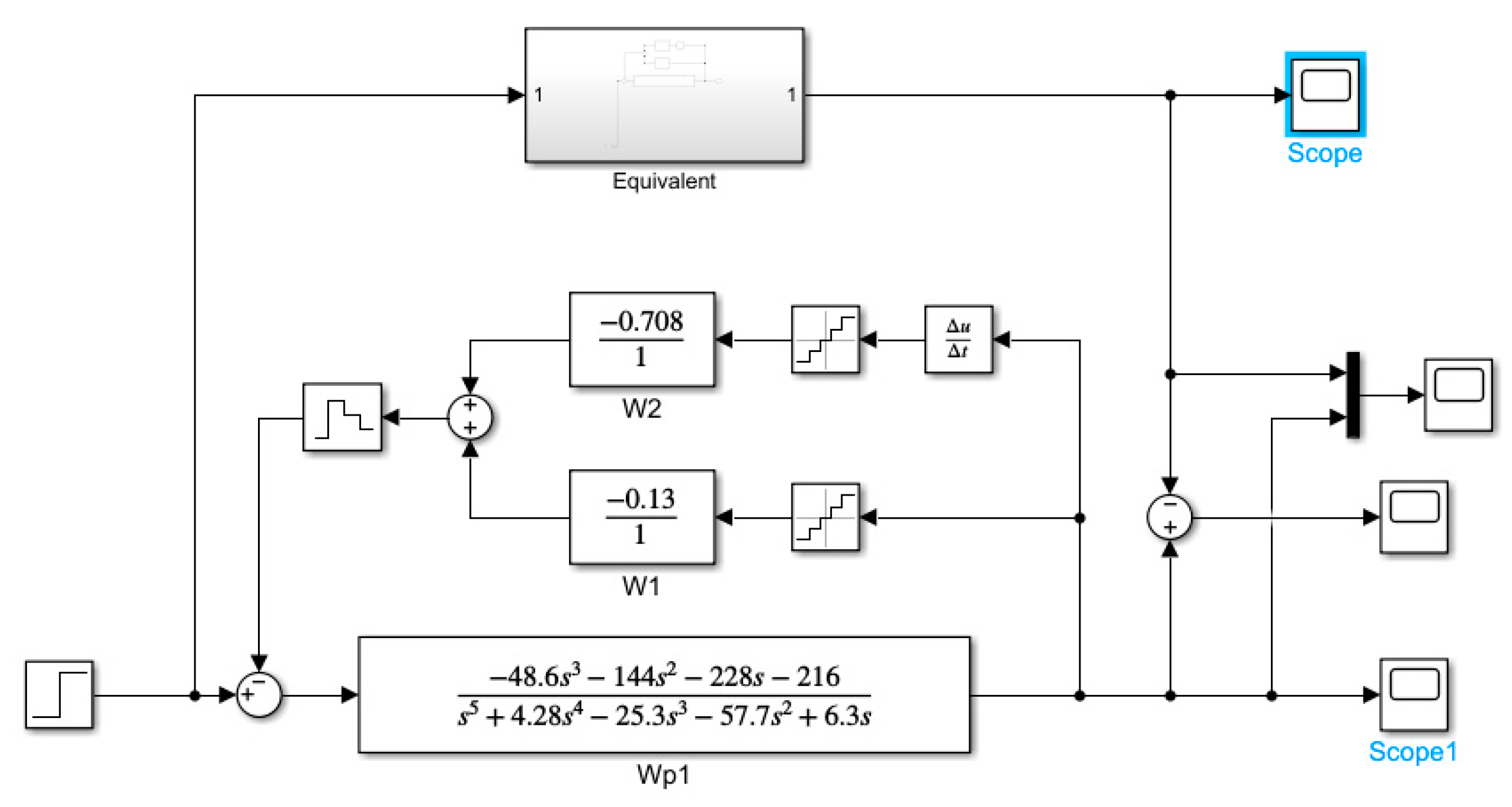
A Simulink calculation scheme is shown in Figure 4.

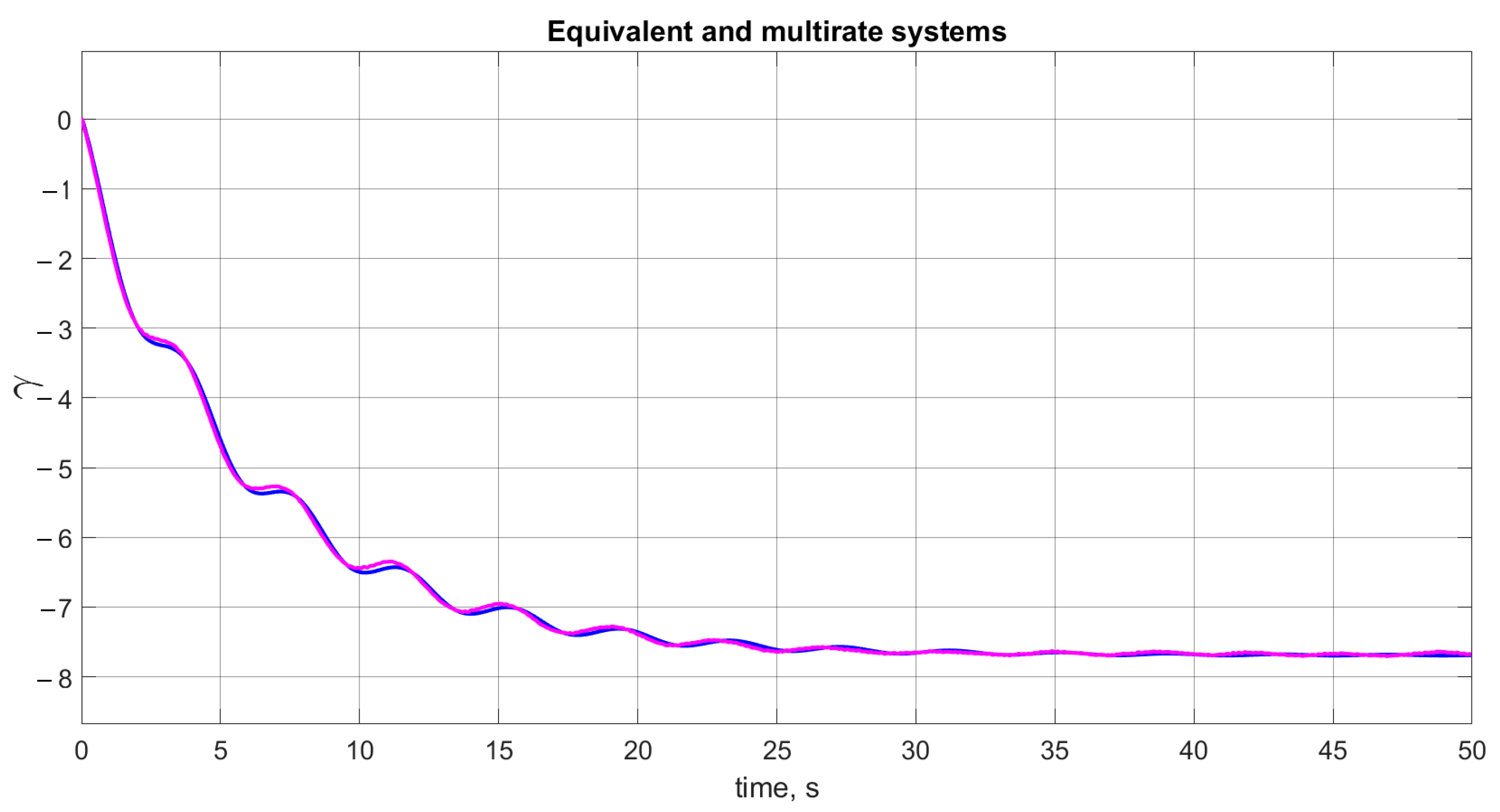
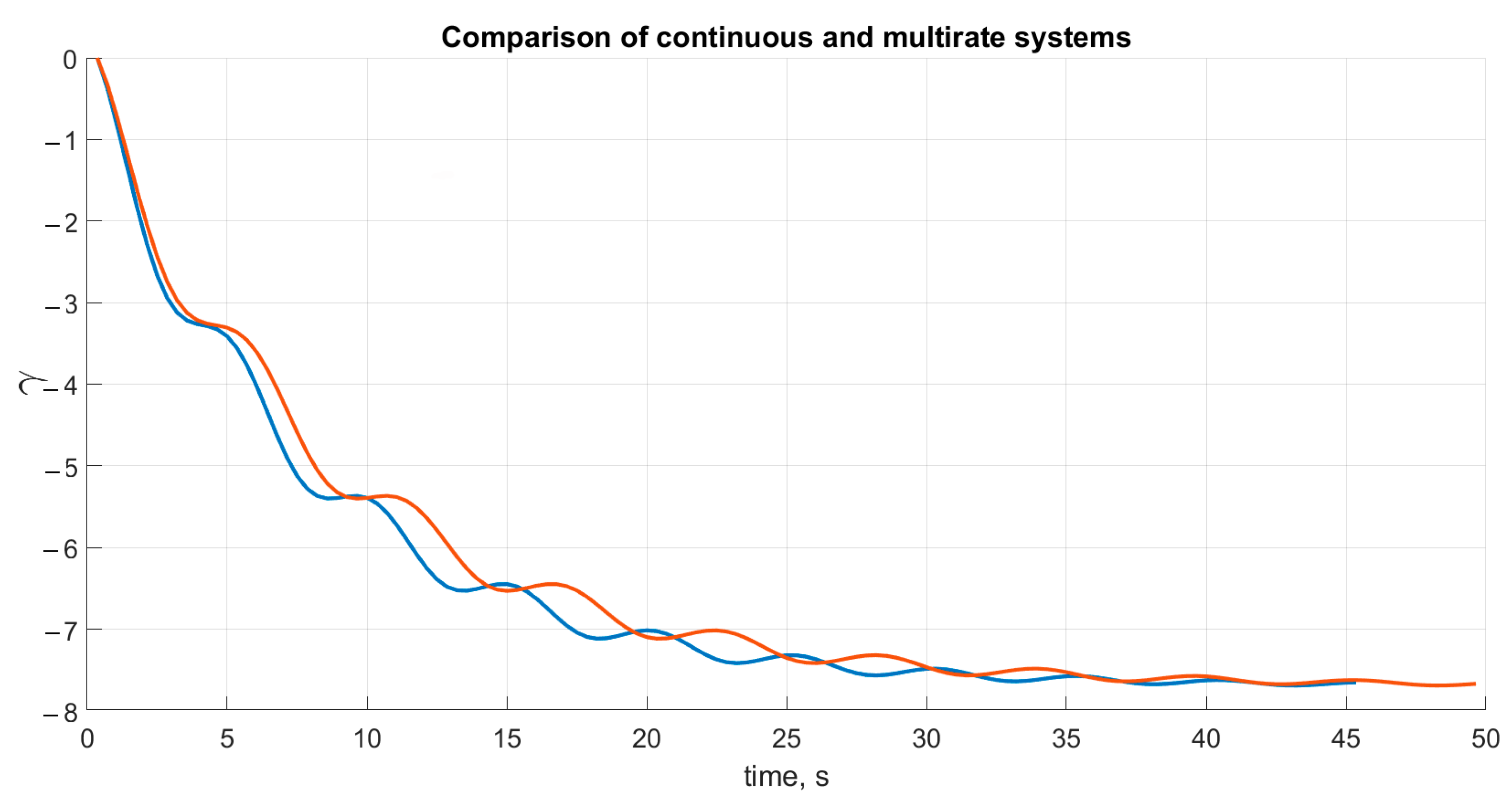
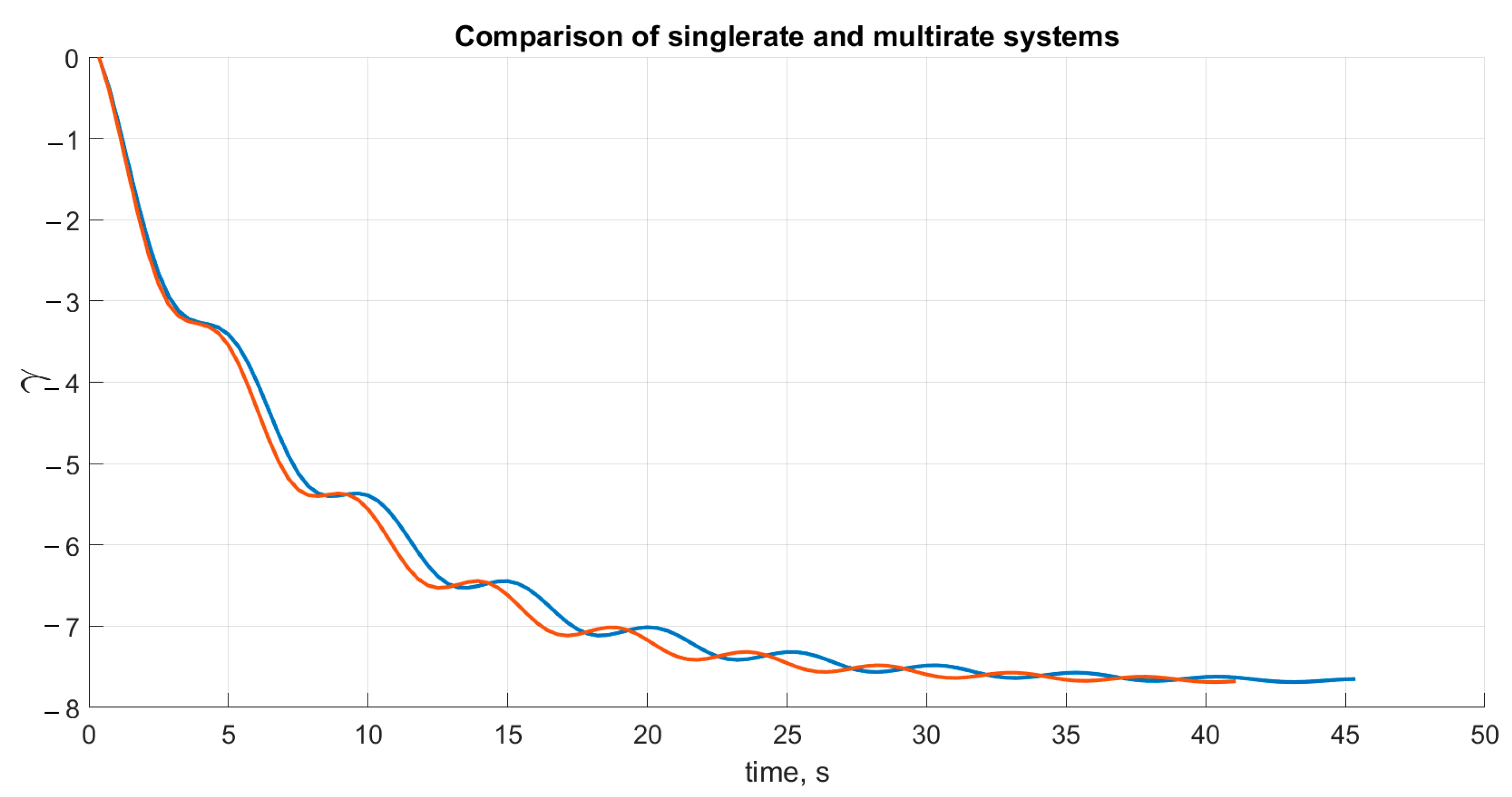
As equivalent models, we will take a continuous system with the same transfer functions, but with continuous circuits in the feedback, a discrete single-rate system with equal sampling periods in feedback loops, and an equivalent system with a sampling period T, which is the greatest common divisor of the sampling periods.

The simulation results are shown in Figure 5, Figure 6, Figure 7 and Figure 8.

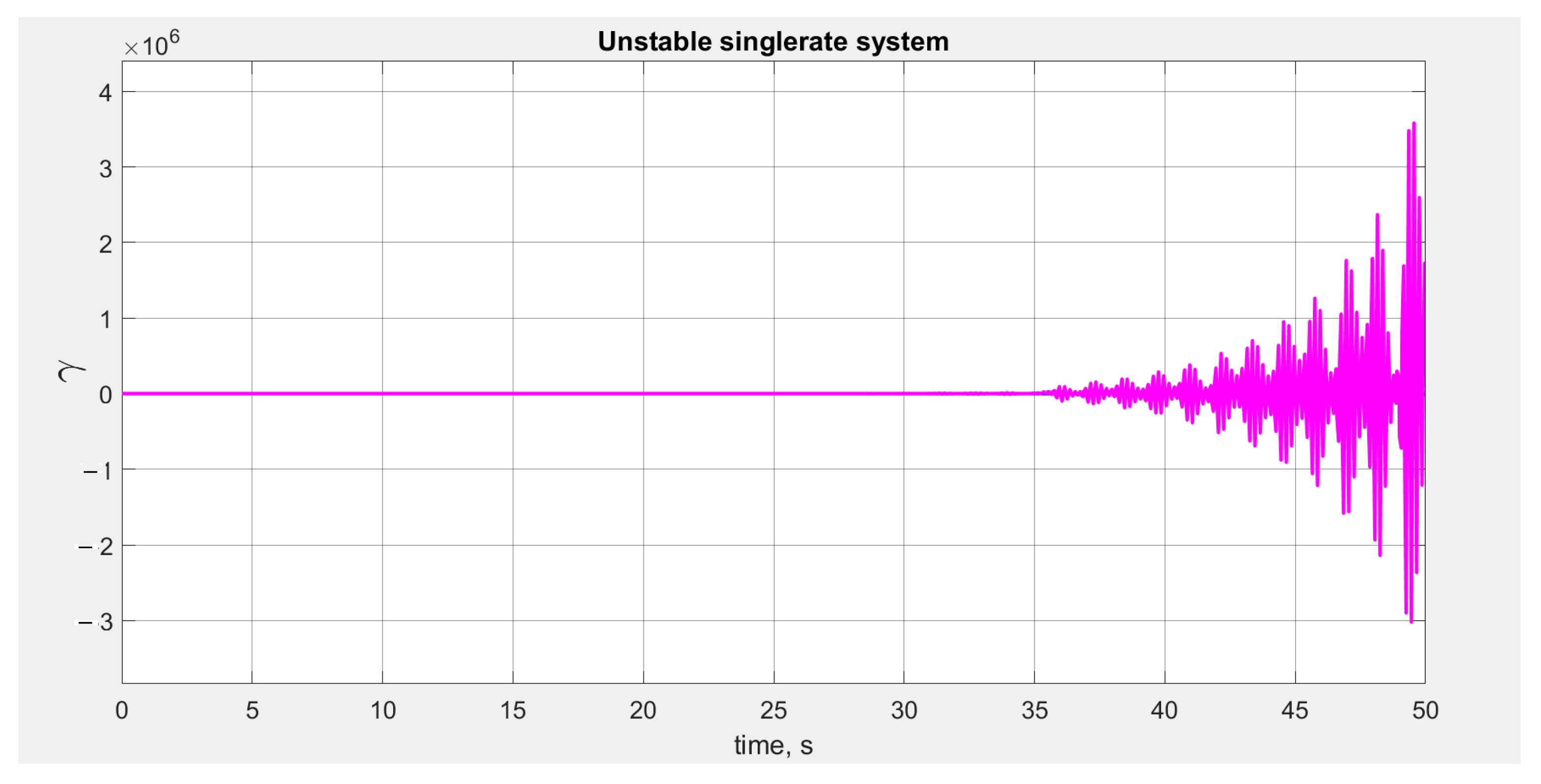
Analyzing the results, we conclude that a simple replacement of a multirate system with a continuous and single-rate system leads to unsatisfactory results. In the case of a single-rate system, the system becomes unstable at certain values of the sampling period. The transient process of the constructed equivalent system practically coincides with the transient process of the original model.

4. Discussion

If the system contains several digital information-processing circuits with different periods, then its study is greatly complicated. In the general case of incommensurate quantization periods, the mathematical apparatus of the study is practically not developed. In the case of rationally commensurate quantization periods (the periods are integer multiples of a certain “effective” period), it is possible to transform a multirate system to an equivalent single-rate of the increased dimension. In the theory of impulse systems, such transformations are usually performed based on parallelizing impulse circuits.

As a result, vector–matrix equivalent single-rate models are obtained using the discrete Laplace transform of MIMO multirate multiloop stabilization systems given by relations (4)–(6), or by structural diagrams, an example of which is shown in Figure 2.

Because of the construction of equivalent mathematical models, it becomes fundamentally possible to transfer the synthesis and analysis methods of continuous MIMO systems to the class of continuous-discrete MIMO multiloop multirate systems.

On the one hand, we obtained an effective tool for constructing an equivalent single-rate form for describing MIMO multiloop multirate stabilization systems, to which the methods of synthesis and analysis of continuous MIMO systems can be extended. On the other hand, implementing the proposed technique leads to cumbersome calculations and work with large transfer function matrices. The dimension of the equivalent system is influenced by the mutual numerical characteristics of digital circuits. Thus, the general construction of the system model complication is indicated due to the increase in the dimension of the equivalent model at significant values of the clock multiplicity numbers and the number of quantization chains. This is illustrated by an example, including constructing a matrix of quantization densities—a structural invariant of quantization chains.

Linear MIMO control systems—systems with multiple inputs and multiple outputs —are part of the linear system class. Therefore, their theory is based on the same foundation as the theory of SISO systems [30,31,32]. If we talk about models of linear systems of a complex domain (domains of Laplace transformations, z-transformations), then this dynamics is determined by the input–output relations in the form of the corresponding rational functions-scalar for a one-dimensional matrix for multidimensional systems. At the same time, the class of multidimensional systems (more complex by the property of multidimensionality) in comparison with the class of one-dimensional systems requires further development of the theory of linear systems, in connection with special mathematical problems of research, which are absent in the class of one-dimensional systems or appear in a much simpler form. Thus, for example, the solution of several problems requires the use of equivalent transformations of polynomial matrices that determine the transfer matrix of the system to a relatively simple form.

Implementing the corresponding computational procedures is a difficult task, the solution of which becomes more complex with an increase in the dimension of the system. Thus, for example, the solution of several problems requires using equivalent transformations of polynomial matrices that determine the transfer matrix of the system to a relatively simple form. Methods for constructing the most significant common divisors of polynomial matrices also play an essential role in implementing these transformations.

5. Conclusions

The input–output model of the system in the domain of discrete Laplace transform is adopted as the initial description in the article. The construction of the matrix of transfer functions of a MIMO system is a difficult task, the solution of which is based on the mathematical apparatus of the theory of polynomial matrices. Considerable attention has been paid to this problem, primarily within the framework of the theory of continuous systems [31,32]. In principle, the methods of this theory can be easily transferred to multidimensional impulse (continuous-discrete) single-rate systems. Therefore, in consideration of multirate continuous-discrete, significant attention is paid to the problem of constructing an equivalent impulse single-rate system, the complete solution of which, as shown, is possible in the case of rationally commensurate quantization periods in the digital circuits of the system.

In all cases, the impulse representations of the outputs of the equivalent T- and NT-models have the form of rational functions of the indicated variables

$$\begin{array}{l}{y}_T^{*}(s)=f(\psi (e^{sT}),\hspace{0.17em}{\psi }_1(e^{s{T}_1}),\dots ,\hspace{0.17em}{\psi }_r(e^{s{T}_r})),\\ y_{NT}^{*}(s)=F(\Psi (e^{sT}),\hspace{0.17em}{\Psi }_1(e^{s{T}_1}),\dots ,\hspace{0.17em}{\Psi }_r(e^{s{T}_r})).\end{array}$$

The solution to this problem fundamentally allows developing methods for analyzing and synthesizing MIMO continuous and discrete systems on a common theoretical basis—the theory of polynomials and rational functions, which are typical elements of the descriptions of these classes of systems.