
Self-Localization of Tethered Drones without a Cable Force Sensor in GPS-Denied Environments


Abstract
:1. Introduction
2. System Dynamics and Accelerometer Principles
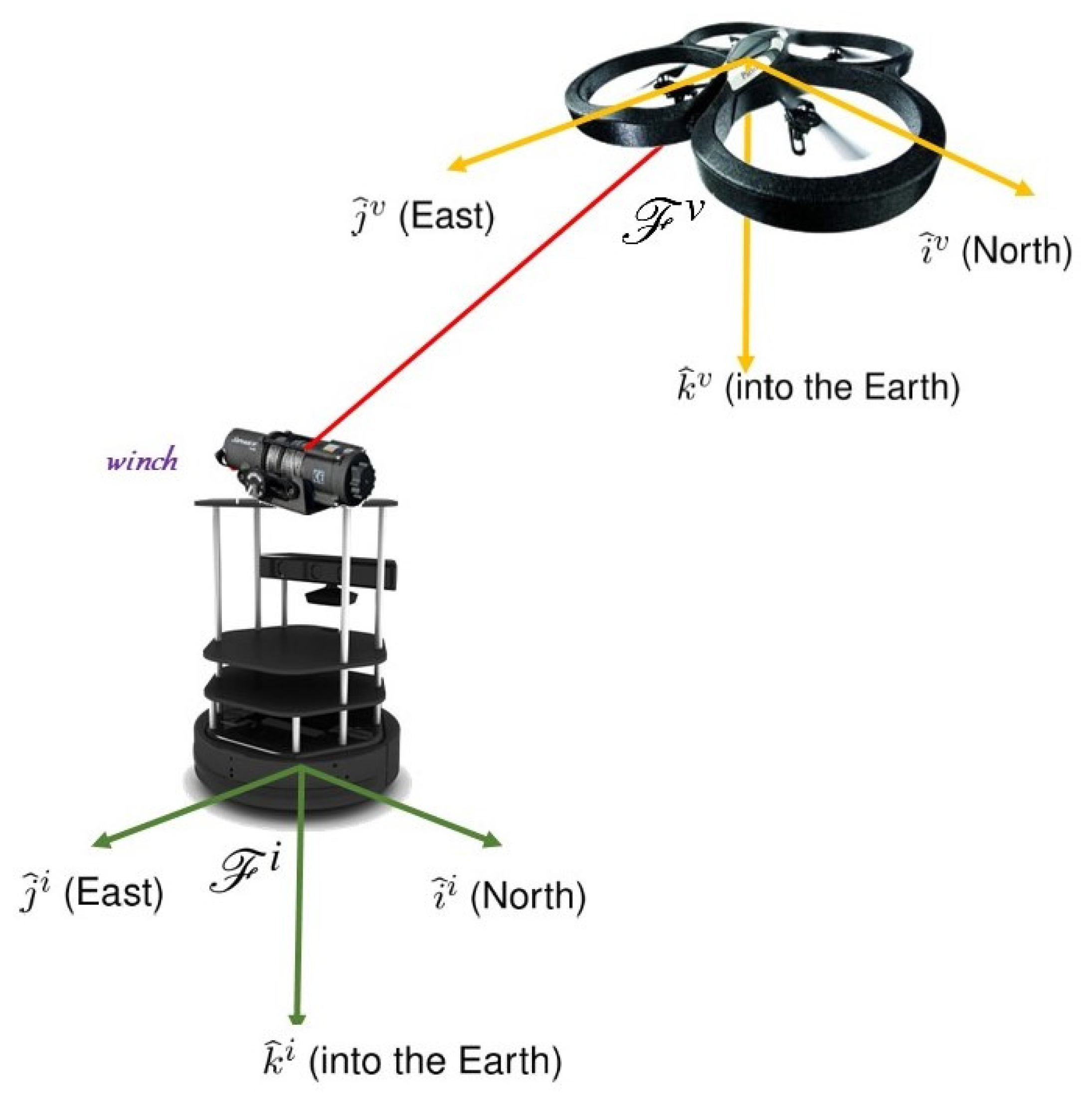
2.1. Coordinate Frames
2.1.1. The Inertial Frame
2.1.2. The Vehicle Frame
2.1.3. The Body Frame
2.2. Tethered Drone Dynamics
2.3. Accelerometer Principle
Kinematic Accelerations and Specific Forces
2.4. External Forces of Tethered Drone
3. Self-Localization of Tethered Drone
3.1. Problem Statement
3.2. State-Space Model for Self-Localization
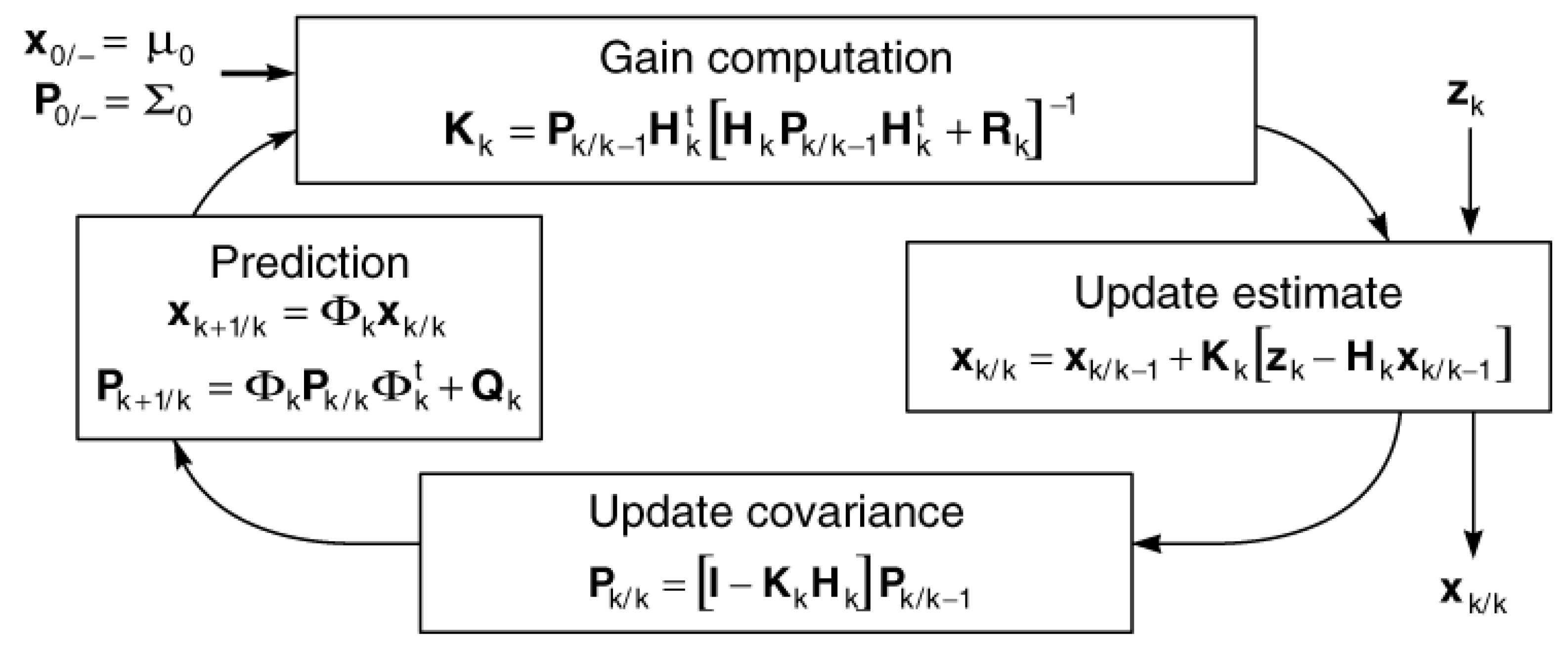
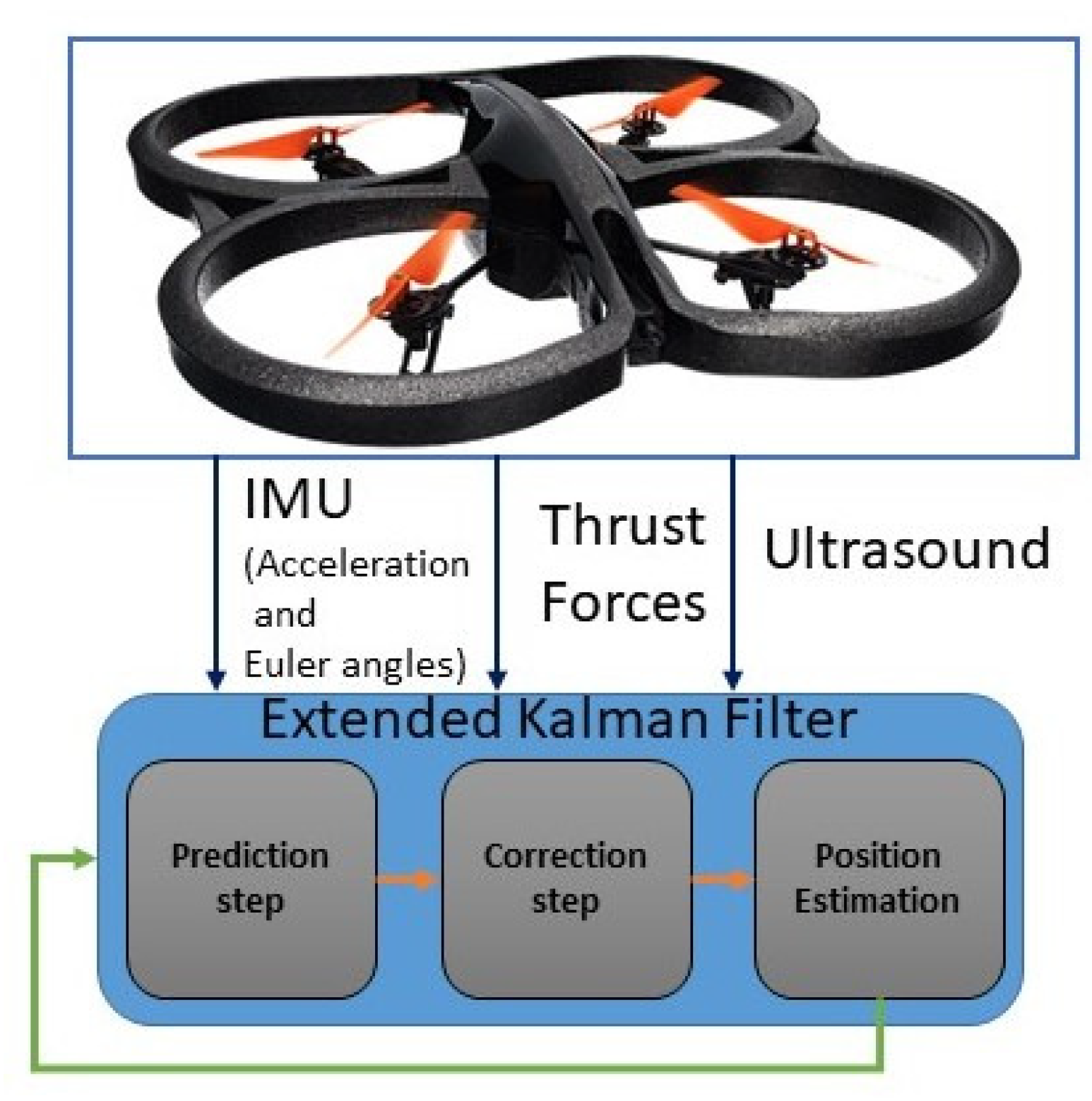
4. Extended Kalman Filter
| Algorithm 1 Extended Kalman Filter [35]. |
1: Initialize: 2: At each sample time , 3: for i = 1 to N do {Prediction} 4: 5: 6: 7: Calculate A, P, and C 8: end for 9: if measurement has been received from sensor i then {Correction:Measurement Update} 10: 11: 12: 13: 14:end if |
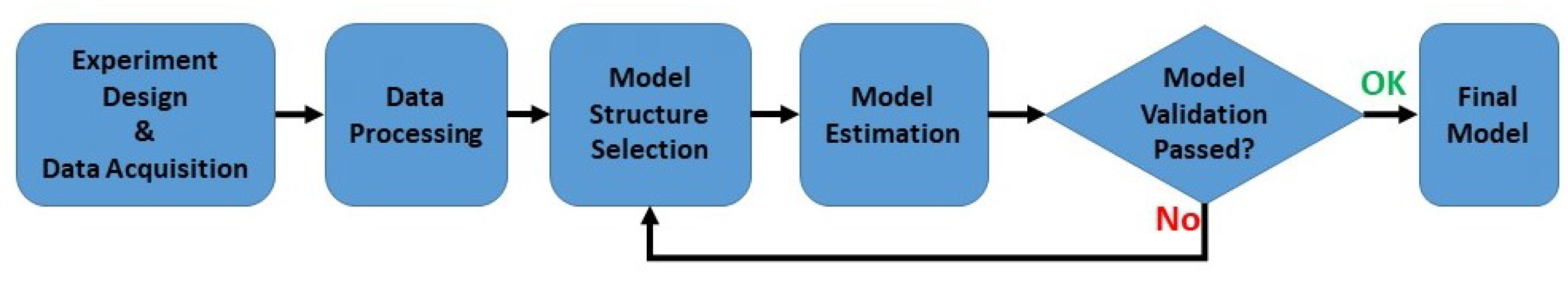
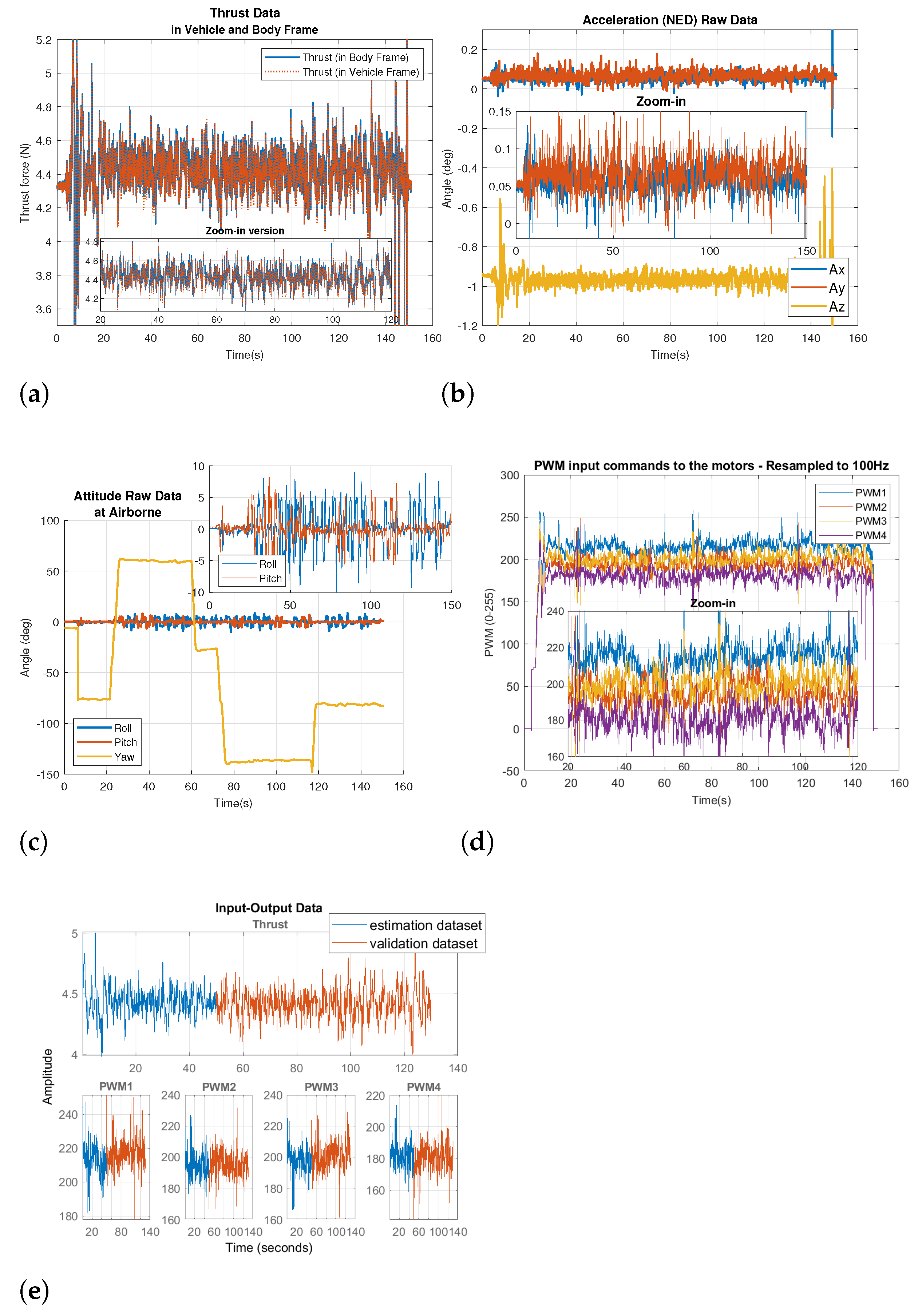
5. System Identification for Motor Coefficients
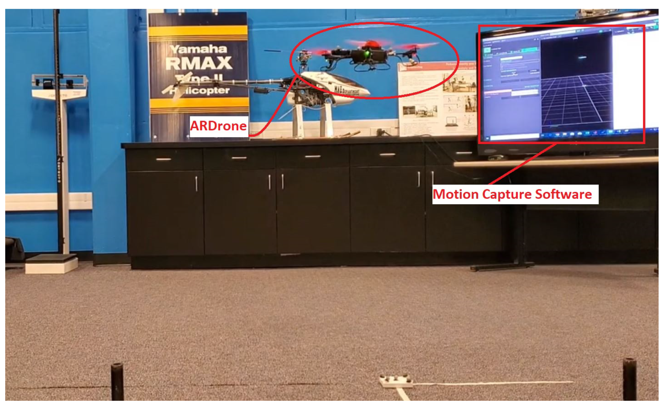
5.1. Experiment Design and Data Acquisition
5.2. Data Processing
5.3. Model Structure Selection, Estimation, and Validation
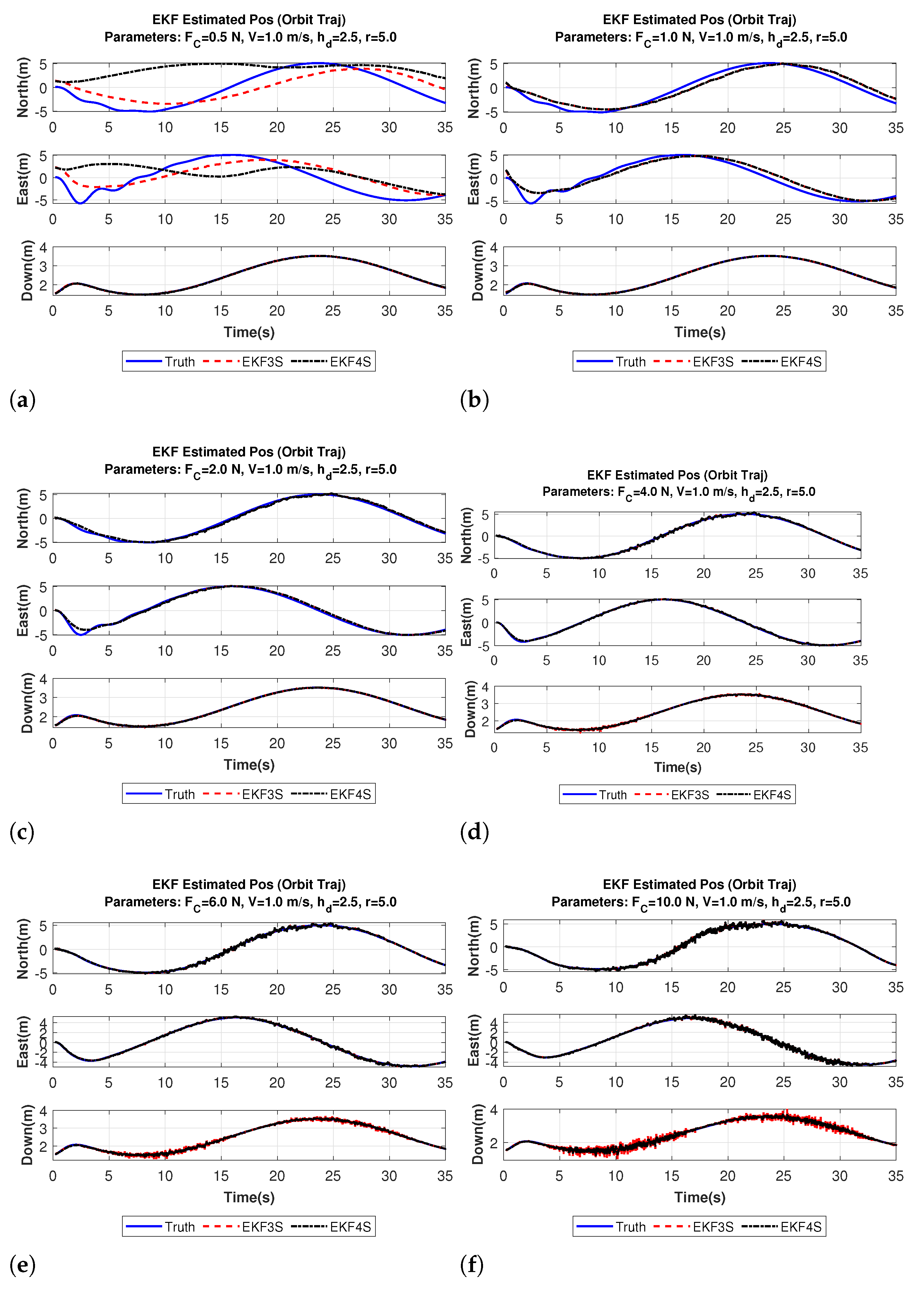
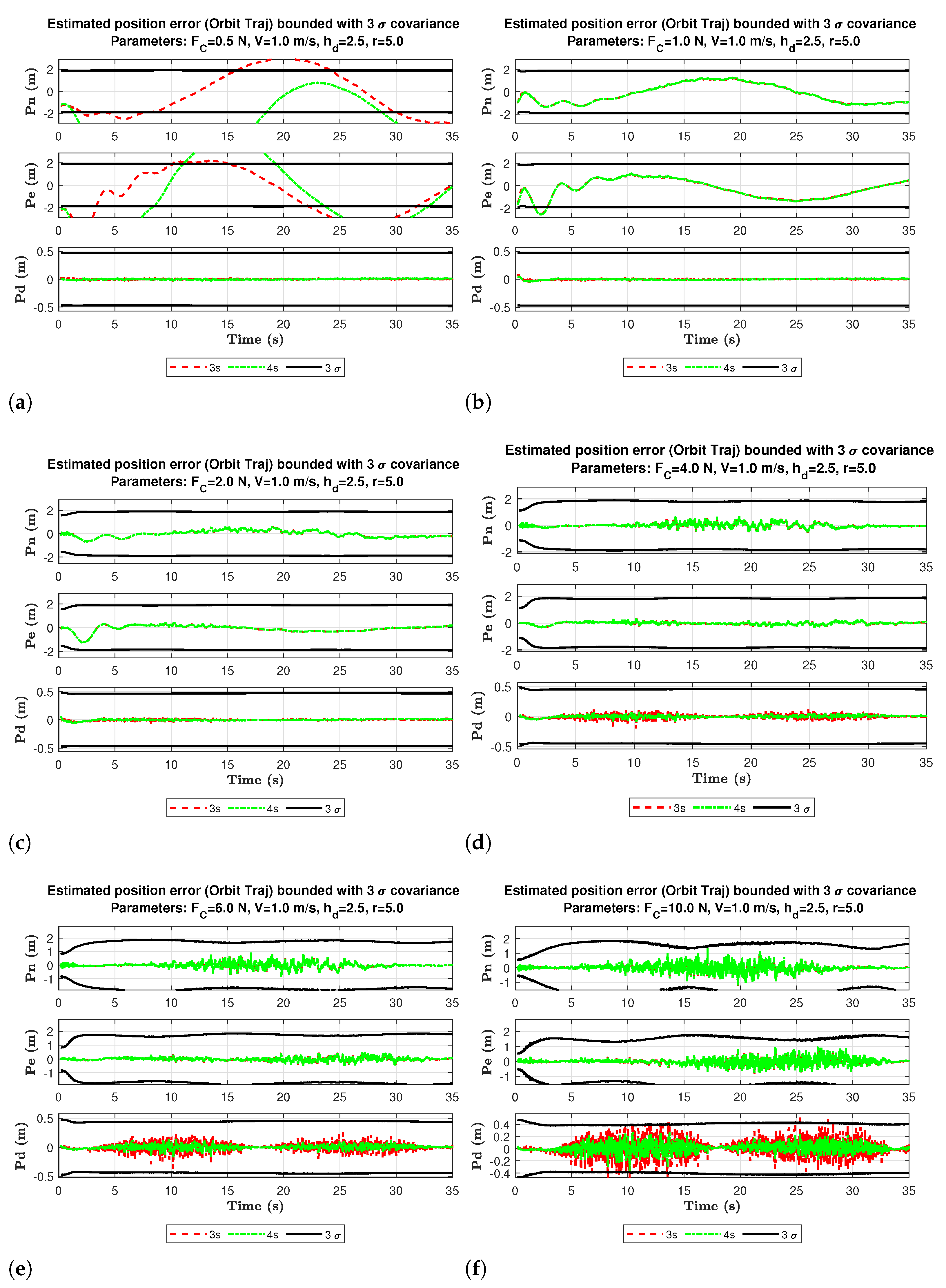
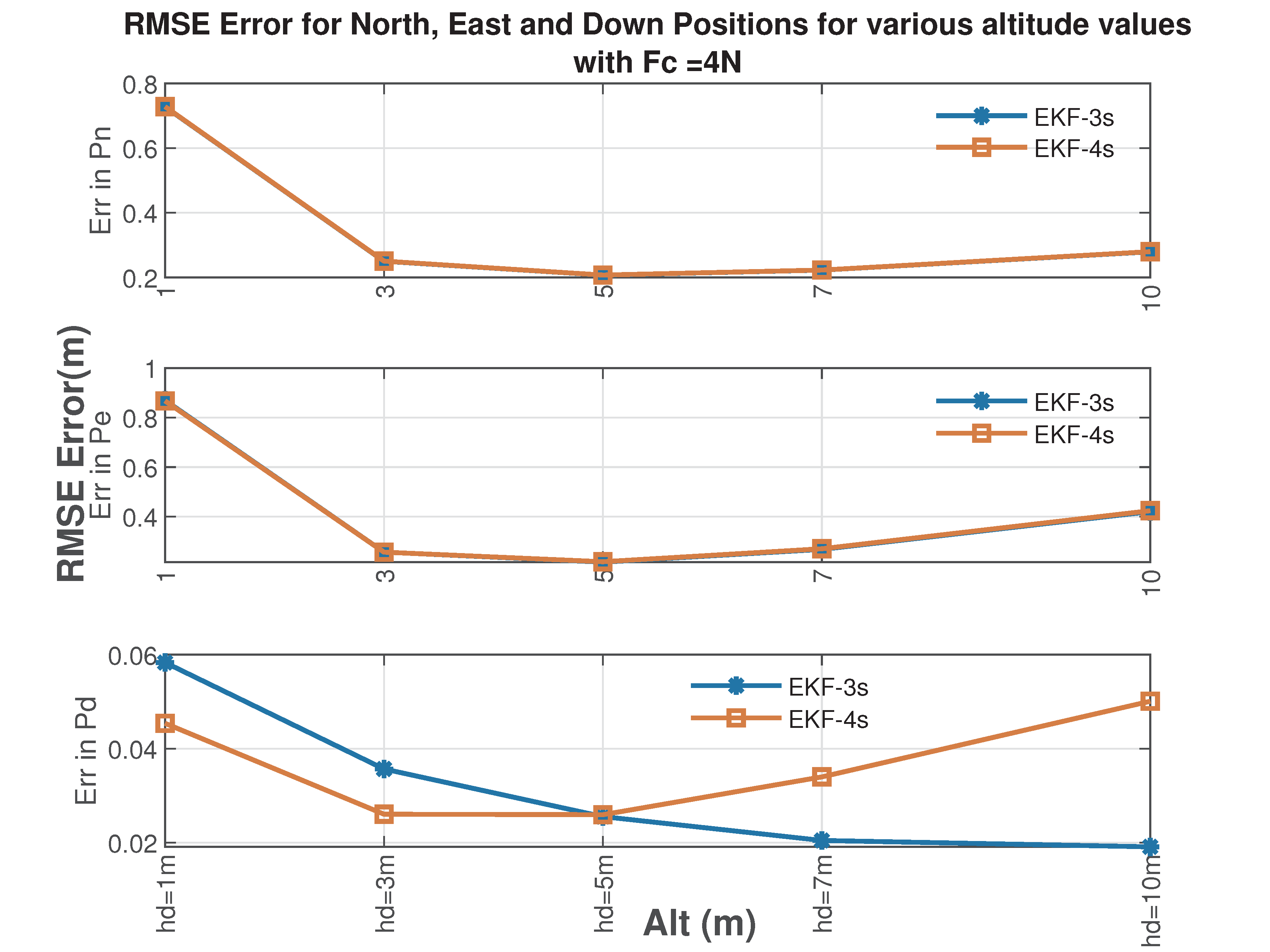
6. Simulation Results and Discussion
7. Conclusions
8. Future Work
Author Contributions
Funding
Institutional Review Board Statement
Informed Consent Statement
Data Availability Statement
Conflicts of Interest
Appendix A
References
- ELISTAIR. Available online: https://elistair.com/orion-tethered-drone/ (accessed on 1 September 2021).
- Prior, S.D. Tethered drones for persistent aerial surveillance applications. In Defence Global; Barclay Media Limited: Manchester, UK, 2015; pp. 78–79. [Google Scholar]
- Al Nuaimi, O.; Almelhi, O.; Almarzooqi, A.; Al Mansoori, A.A.S.; Sayadi, S.; Swamidoss, I. Persistent surveillance with small Unmanned Aerial Vehicles (sUAV): A feasibility study. In Electro-Optical Remote Sensing XII; International Society for Optics and Photonics: Berlin, Germany, 2018; Volume 10796, p. 107960K. [Google Scholar]
- Tarchi, D.; Guglieri, G.; Vespe, M.; Gioia, C.; Sermi, F.; Kyovtorov, V. Search and rescue: Surveillance support from RPAs radar. In Proceedings of the 2017 European Navigation Conference (ENC), Lausanne, Switzerland, 9–12 May 2017; pp. 256–264. [Google Scholar]
- Dorn, L. Heavy Duty Tethered Cleaning Drones That Safely Wash Windows of High Altitude Skyscrapers. 2021. Available online: https://laughingsquid.com/aerones-skyscraper-window-washing-drone/ (accessed on 1 September 2021).
- Kumparak, G. Lucid’s Drone Is Built to Clean the Outside of Your House or Office. 2019. Available online: https://techcrunch.com/2019/08/27/lucids-drone-is-built-to-clean-the-outside-of-your-house-or-office/ (accessed on 1 September 2021).
- What Are the Benefits of Tethered Drones? 2021. Available online: https://elistair.com/tethered-drones-benefits/ (accessed on 1 September 2021).
- This Drone Can Clean Wind Turbines. 2018. Available online: https://www.irishnews.com/magazine/technology/2018/03/27/news/this-drone-can-clean-wind-turbines-1289122/ (accessed on 1 September 2021).
- Drones and Robots that Clean Wind Turbines. 2021. Available online: https://www.nanalyze.com/2019/12/drones-robots-clean-wind-turbines/ (accessed on 1 September 2021).
- Reagan, P.B.J. Fotokite Launches Tethered Drone System for Firefighters. 2019. Available online: https://dronelife.com/2019/04/17/fotokite-launches-tethered-drone-system-for-firefighters/ (accessed on 1 September 2021).
- Estrada, C.; Sun, L. Trajectory Tracking Control of a Drone-Guided Hose System for Fluid Delivery. In Proceedings of the AIAA Scitech 2021 Forum, Nashville, TN, USA, 11–15 January 2021; p. 1003. [Google Scholar]
- Al-Radaideh, A.; Al-Jarrah, M.; Jhemi, A. UAV testbed building and development for research purposes at the american university of sharjah. In Proceedings of the ISMA’10 7th International Symposium on Mechatronics and Its Applications, Sharjah, United Arab Emirates, 20–22 April 2010. [Google Scholar]
- Al-Radaideh, A. Guidance, Control and Trajectory Tracking of Small Fixed Wing Unmanned Aerial Vehicles (UAV’s) A THESIS IN MECHATRONICS. Master’s Thesis, American University of Sharjah, Sharjah, United Arab Emirates, 2009. [Google Scholar]
- Al-Radaideh, A.; Al-Jarrah, M.A.; Jhemi, A.; Dhaouadi, R. ARF60 AUS-UAV modeling, system identification, guidance and control: Validation through hardware in the loop simulation. In Proceedings of the 2009 6th International Symposium on Mechatronics and Its Applications, Sharjah, United Arab Emirates, 23–26 March 2009; pp. 1–11. [Google Scholar]
- Martin, P.; Salaün, E. The true role of accelerometer feedback in quadrotor control. In Proceedings of the 2010 IEEE International Conference on Robotics and Automation, Anchorage, AK, USA, 3–7 May 2010; pp. 1623–1629. [Google Scholar]
- Hoffmann, G.; Huang, H.; Waslander, S.; Tomlin, C. Quadrotor helicopter flight dynamics and control: Theory and experiment. In Proceedings of the AIAA Guidance, Navigation, and Control Conference and Exhibit, San Francisco, CA, USA, 15–18 August 2007. [Google Scholar]
- Escareno, J.; Salazar-Cruz, S.; Lozano, R. Embedded control of a four-rotor UAV. In Proceedings of the 2006 American Control Conference, Minneapolis, MN, USA, 14–16 June 2006. [Google Scholar] [CrossRef]
- He, R.; Prentice, S.; Roy, N. Planning in information space for a quadrotor helicopter in a GPS-denied environment. In Proceedings of the 2008 IEEE International Conference on Robotics and Automation, Pasadena, CA, USA, 19–23 May 2008; pp. 1814–1820. [Google Scholar] [CrossRef] [Green Version]
- Grzonka, S.; Grisetti, G.; Burgard, W. Towards a navigation system for autonomous indoor flying. In Proceedings of the 2009 IEEE International Conference on Robotics and Automation, Kobe, Japan, 12–17 May 2009; pp. 2878–2883. [Google Scholar]
- Bouabdallah, S.; Siegwart, R. Full control of a quadrotor. In Proceedings of the 2007 IEEE/RSJ International Conference on Intelligent Robots and Systems, San Diego, CA, USA, 29 October–2 November 2007; pp. 153–158. [Google Scholar]
- Guenard, N.; Hamel, T.; Mahony, R. A practical visual servo control for an unmanned aerial vehicle. IEEE Trans. Robot. 2008, 24, 331–340. [Google Scholar] [CrossRef] [Green Version]
- Kendoul, F.; Fantoni, I.; Nonami, K. Optic flow-based vision system for autonomous 3D localization and control of small aerial vehicles. Robot. Auton. Syst. 2009, 57, 591–602. [Google Scholar] [CrossRef] [Green Version]
- Xu, Q.; Wang, Z.; Gerber, A.; Mao, Z.M. Cellular Data Network Infrastructure Characterization and Implication on Mobile Content Placement. In Proceedings of the ACM SIGMETRICS 2011 International Conference on Measurement and Modeling of Computer Systems, San Jose, CA, USA, 7–11 June 2011; pp. 317–328. [Google Scholar]
- Lupashin, S.; D’Andrea, R. Stabilization of a flying vehicle on a taut tether using inertial sensing. In Proceedings of the 2013 IEEE/RSJ International Conference on Intelligent Robots and Systems, Tokyo, Japan, 3–7 November 2013; pp. 2432–2438. [Google Scholar] [CrossRef]
- Tognon, M.; Dash, S.S.; Franchi, A. Observer-Based Control of Position and Tension for an Aerial Robot Tethered to a Moving Platform. IEEE Robot. Autom. Lett. 2016, 1, 732–737. [Google Scholar] [CrossRef] [Green Version]
- Lima, R.R.; Pereira, G.A. On the Development of a Tether-based Drone Localization System. In Proceedings of the 2021 International Conference on Unmanned Aircraft Systems (ICUAS), Athens, Greece, 15–18 June 2021; pp. 195–201. [Google Scholar]
- Amalthea, A. World Premier: Tethered Drones at Paris Airports. Available online: https://elistair.com/tethered-drone-at-paris-airports/ (accessed on 1 September 2021).
- Hoverfly—Tethered Drone Technology for Infinite Flight Time. Available online: https://hoverflytech.com/ (accessed on 1 September 2021).
- Al-Radaidehl, A.; Sun, L. Observability Analysis and Bayesian Filtering for Self-Localization of a Tethered Multicopter in GPS-Denied Environments. In Proceedings of the 2019 International Conference on Unmanned Aircraft Systems (ICUAS), Atlanta, GA, USA, 11–14 June 2019; pp. 1041–1047. [Google Scholar]
- Al-Radaideh, A.; Sun, L. Self-localization of a tethered quadcopter using inertial sensors in a GPS-denied environment. In Proceedings of the 2017 International Conference on Unmanned Aircraft Systems (ICUAS), Miami, FL, USA, 13–16 June 2017; pp. 271–277. [Google Scholar] [CrossRef]
- Jeurgens, N.L.M. Implementing a Simulink controller in an AR. Drone 2.0. Master’s Thesis, Eindhoven University of Technology, Eindhoven, The Netherlands, 2016. [Google Scholar]
- Capello, E.; Park, H.; Tavora, B.; Guglieri, G.; Romano, M. Modeling and experimental parameter identification of a multicopter via a compound pendulum test rig. In Proceedings of the 2015 Workshop on Research, Education and Development of Unmanned Aerial Systems (RED-UAS), Cancun, Mexico, 23–25 November 2015; pp. 308–317. [Google Scholar]
- Chovancová, A.; Fico, T.; Chovanec, L.; Hubinsk, P. Mathematical modelling and parameter identification of quadrotor (a survey). Procedia Eng. 2014, 96, 172–181. [Google Scholar] [CrossRef] [Green Version]
- Elsamanty, M.; Khalifa, A.; Fanni, M.; Ramadan, A.; Abo-Ismail, A. Methodology for identifying quadrotor parameters, attitude estimation and control. In Proceedings of the 2013 IEEE/ASME International Conference on Advanced Intelligent Mechatronics, Wollongong, NSW, Australia, 9–12 July 2013; pp. 1343–1348. [Google Scholar]
- Beard, R.W.; McLain, T.W. Small Unmanned Aircraft: Theory and Practice; Princeton University Press: Princeton, NJ, USA, 2012. [Google Scholar]
- Rauw, M.O. FDC 1.2-A Simulink Toolbox for Flight Dynamics and Control Analysis; Delft University of Technology: Delft, The Netherlands, 2001; pp. 1–7. [Google Scholar]
- Levy, L.J. The Kalman filter: Navigation’s integration workhorse. GPS World 1997, 8, 65–71. [Google Scholar]
- Orderud, F. Comparison of Kalman Filter Estimation Approaches for State Space Models with Nonlinear Measurements; Fagbokforlaget Vigmostad & Bjorke AS: Trondheim, Norway, 2005; pp. 1–8. [Google Scholar]
- Angarita, J.E.; Schroeder, K.; Black, J. Quadrotor Model Generation using System Identification Techniques. In Proceedings of the 2018 AIAA Modeling and Simulation Technologies Conference, Kissimmee, FL, USA, 8–12 January 2018; p. 1917. [Google Scholar]
- Ljung, L. Approaches to identification of nonlinear systems. In Proceedings of the 29th Chinese Control Conference, Beijing, China, 29–31 July 2010; pp. 1–5. [Google Scholar]
- Ljung, L. Identification of Nonlinear Systems; Linköping University Electronic Press: Linköping, Sweden, 2007. [Google Scholar]
- Al-Radaideh, A.; Jhemi, A.; Al-Jarrah, M.A. System identification of the Joker-3 unmanned helicopter. In Proceedings of the AIAA Modeling and Simulation Technologies Conference, Minneapolis, MN, USA, 13–16 August 2012; p. 4725. [Google Scholar]
- Simmons, B.M. System Identification of a Nonlinear Flight Dynamics Model for a Small, Fixed-Wing UAV. Ph.D. Thesis, Virginia Tech, Blacksburg, Virginia, 2018. [Google Scholar]
- Andersson, L.; Jönsson, U.; Johansson, K.H.; Bengtsson, J. A Manual for System Identification; Laboratory Exercises in System Identification. KF Sigma i Lund AB. Department of Automatic Control, Lund Institute of Technology: Lund, Sweden, 2006; Volume 118. [Google Scholar]
- L’Erario, G.; Fiorio, L.; Nava, G.; Bergonti, F.; Mohamed, H.A.O.; Benenati, E.; Traversaro, S.; Pucci, D. Modeling, Identification and Control of Model Jet Engines for Jet Powered Robotics. IEEE Robot. Autom. Lett. 2020, 5, 2070–2077. [Google Scholar] [CrossRef] [Green Version]
- Ljung, L. System Identification Toolbox. Getting Started Guide Release 2017; The MathWorks, Inc.: Natick, MA, USA, 2017. [Google Scholar]
- Ljung, L. Identification for control: Simple process models. In Proceedings of the 41st IEEE Conference on Decision and Control, Las Vegas, NV, USA, 10–13 December 2002; Volume 4, pp. 4652–4657. [Google Scholar]
- Jones, R.H. Fitting autoregressions. J. Am. Stat. Assoc. 1975, 70, 590–592. [Google Scholar]
- Poli, A.A.; Cirillo, M.C. On the use of the normalized mean square error in evaluating dispersion model performance. Atmos. Environ. Part A Gen. Top. 1993, 27, 2427–2434. [Google Scholar] [CrossRef]
- Monajjemi, M. Ardrone Autonomy: A Ros Driver for Ardrone 1.0 & 2.0. 2012. Available online: https://github.com/AutonomyLab/ardrone_autonomy (accessed on 1 September 2021).


| Structure | Fit% | FPE | MSE |
|---|---|---|---|
| Transfer Function (mtf) | 46% | 0.002388 | 0.002343 |
| Process Model (midproc0) | 41.41% | 0.002796 | 0.002778 |
| Black-Box model-ARX Model (marx) | 96.77% | 8.478 × | 8.438 × |
| State-Space Models Using (mn4sid) | 99.56% | 1.589 × | 1.562 × |
| Box-Jenkins Model (bj) | 94.64% | 2.339 × | 2.326 × |
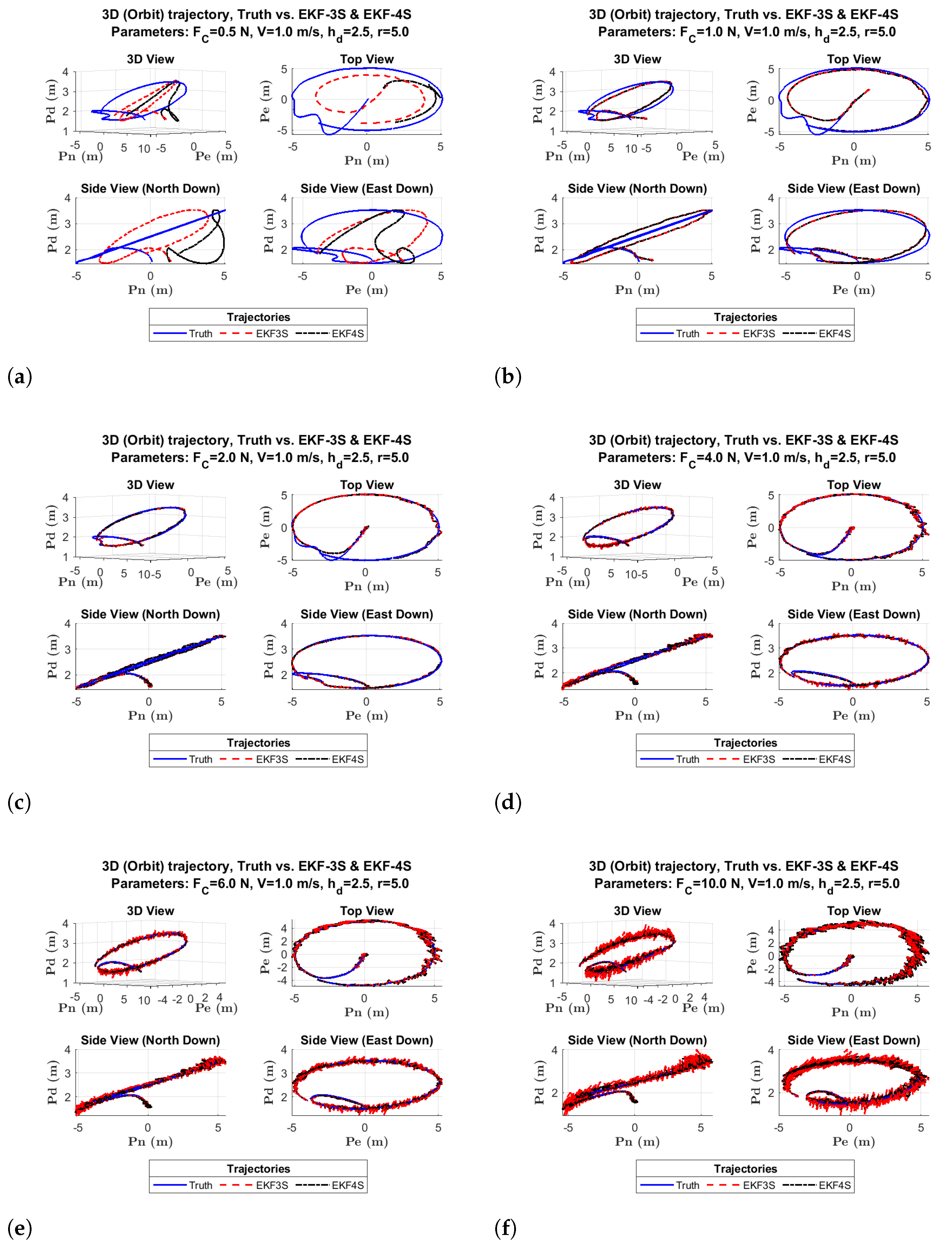
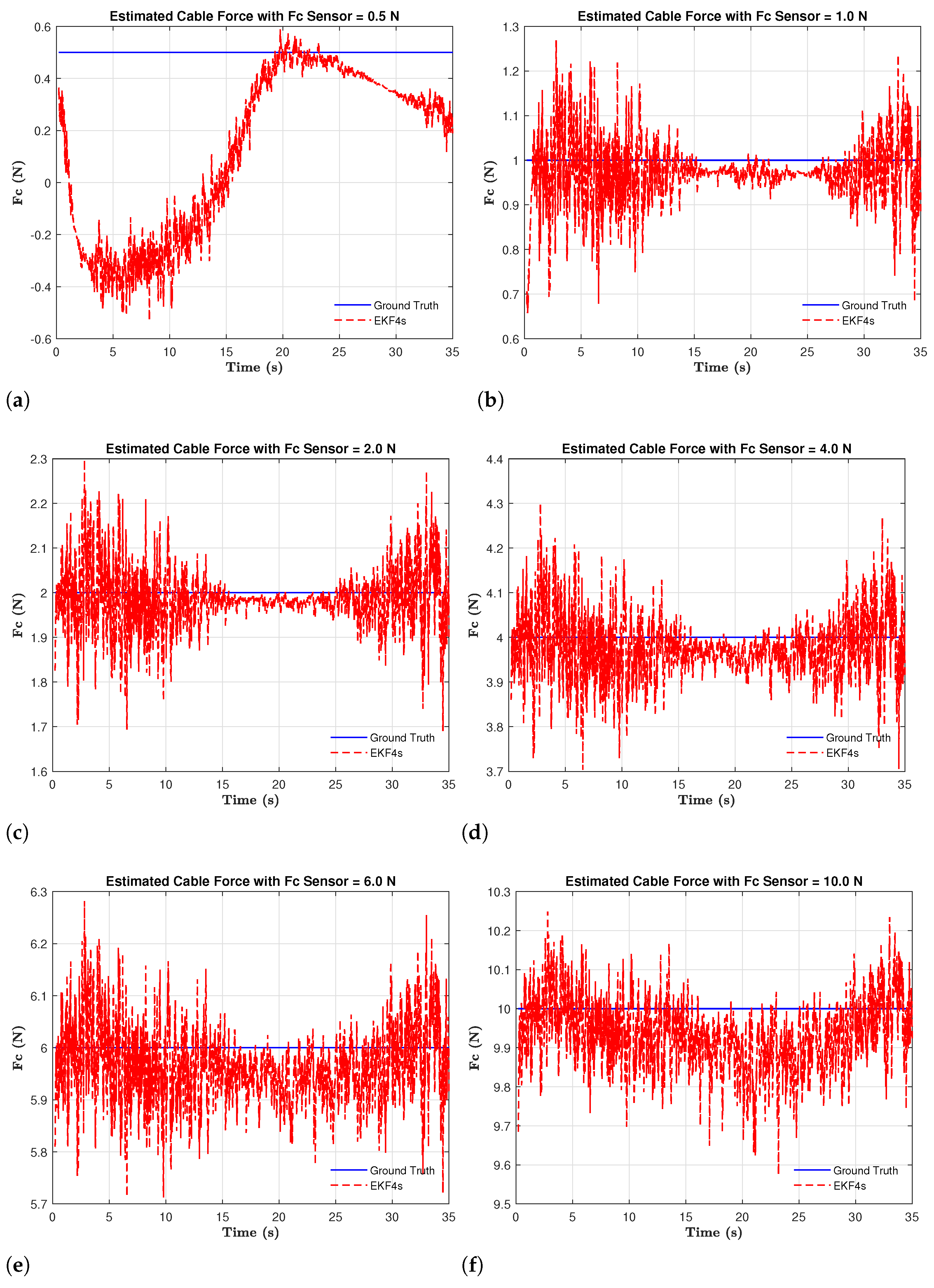
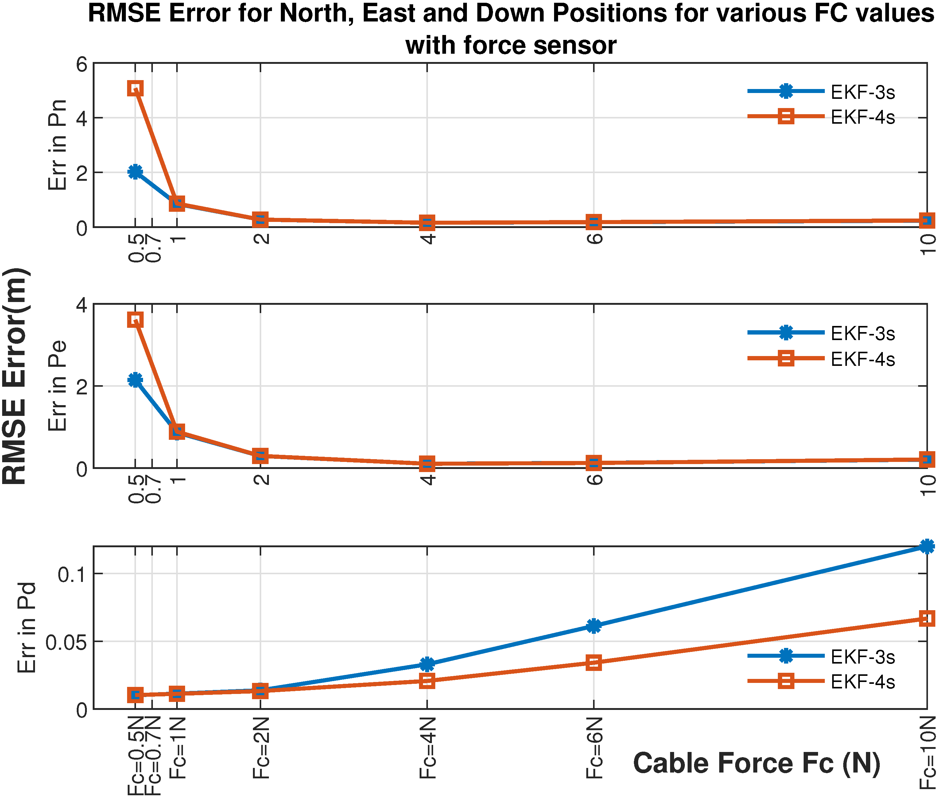
| 0.5 N | 2 N | 4 N | 10 N | |||||
|---|---|---|---|---|---|---|---|---|
| Position | 3S | 4S | 3S | 4S | 3S | 4S | 3S | 4S |
| North (m) | 2.022 | 5.075 | 0.275 | 0.276 | 0.159 | 0.156 | 0.236 | 0.243 |
| East (m) | 2.146 | 3.613 | 0.294 | 0.296 | 0.106 | 0.105 | 0.206 | 0.209 |
| Down (m) | 0.010 | 0.010 | 0.014 | 0.013 | 0.033 | 0.020 | 0.120 | 0.067 |
| (N) | - | 0.495 | - | 0.066 | - | 0.071 | - | 0.109 |
Publisher’s Note: MDPI stays neutral with regard to jurisdictional claims in published maps and institutional affiliations. |
© 2021 by the authors. Licensee MDPI, Basel, Switzerland. This article is an open access article distributed under the terms and conditions of the Creative Commons Attribution (CC BY) license (https://creativecommons.org/licenses/by/4.0/).
Share and Cite
Al-Radaideh, A.; Sun, L. Self-Localization of Tethered Drones without a Cable Force Sensor in GPS-Denied Environments. Drones 2021, 5, 135. https://doi.org/10.3390/drones5040135
Al-Radaideh A, Sun L. Self-Localization of Tethered Drones without a Cable Force Sensor in GPS-Denied Environments. Drones. 2021; 5(4):135. https://doi.org/10.3390/drones5040135
Chicago/Turabian StyleAl-Radaideh, Amer, and Liang Sun. 2021. "Self-Localization of Tethered Drones without a Cable Force Sensor in GPS-Denied Environments" Drones 5, no. 4: 135. https://doi.org/10.3390/drones5040135
APA StyleAl-Radaideh, A., & Sun, L. (2021). Self-Localization of Tethered Drones without a Cable Force Sensor in GPS-Denied Environments. Drones, 5(4), 135. https://doi.org/10.3390/drones5040135