

Advanced Leak Detection and Quantification of Methane Emissions Using sUAS


Abstract
:1. Introduction
2. Problem Overview
3. Sensors and Equipment
4. Advanced Leak Detection and Quantification Methods
4.1. Simulation-Based
4.1.1. Forward Modeling
4.1.2. Backward Lagrangian Stochastic (bLS)
4.1.3. Mesoscale Recursive Bayesian Least Squares Inverse (RB-LSI)
4.2. Optimization-Based
4.2.1. Point Source Gaussian (PSG)—OTM33A
4.2.2. Conditionally Sampled PSG (PSG-CS)
4.2.3. Recursive Bayesian Point Source Gaussian Method (PSG-RB)
4.2.4. Point Source Gaussian Sequential Bayesian Markov Chain Monte Carlo (PSG-SBM)
4.2.5. Near-Field Gaussian Plume Inversion (NGI)
4.3. Mass Balance Based
4.3.1. Vertical Flux Plane (VFP)
4.3.2. Cylindrical Flux Plane (CFP)
4.3.3. Path Integrated Vertical Flux Plane (PI-VFP)
4.3.4. Micrometeorological Mass Difference (MMD)
4.3.5. Gauss Divergence Theorem (GDT)
4.3.6. Vertical Flux Planes with GLM (GLM-VFP)
4.3.7. Vertical Radial Plume Mapping (VRPM)
4.4. Imaging-Based
4.4.1. Mid-Wave Infrared (MWIR) and Hyperspectral
4.4.2. Iterative Maximum a Posteriori Differential Optical Absorption Spectroscopy (IMAP-DOAS)
4.5. Correlation-Based
4.5.1. Tracer Correlation (TCM)
4.5.2. Eddy Covariance (EC)
5. Analysis of Methods and Assessment
6. Summary of Methods
7. Future Directions
8. Conclusions
Author Contributions
Funding
Acknowledgments
Conflicts of Interest
Abbreviations
| ADE | Advection diffusion equation |
| AJAX | Alpha Jet Atmospheric eXperiment |
| ALD | Advance Leak Detection |
| AMFC | Alberta Methane Field Challenge |
| AMOG | AutoMObile greenhouse Gas |
| ARPA-E | Advanced Research Projects Agency-Energy |
| AVIRIS-NG | Next generation Airborne visible/infrared imaging spectrometer |
| bLS | Backward Lagrangian Stochastic dispersion technique |
| bs-TDLAS | Back scatter tunable diode laser absorption spectrometer |
| CALMIM | California Landfill Methane Inventory Model |
| CARB | California Air Resources Board |
| CASIE | Characterization of Arctic Sea Ice Experiment |
| CFP | Cylindrical Flux Plane |
| CRDS | Cavity ring-down spectrometer |
| DiAL | Differential Absorption LiDAR Method |
| DT | Digital Twin |
| EC | Eddy Covariance |
| EDF | Environmental Defense Fund |
| EPA | Environmental Protection agency |
| EPA FLIGHT | EPA Facility Level Informationon Greenhouse gases Tool |
| FEAST | Fugitive Emissions Abatement Simulation Toolkit |
| FID | Flame Ionization Detector |
| FLEXPART-WRF | FLEXible PARTicle-Weather Research and Forecasting |
| FPE | Fokker–Planck equation |
| FTIR | Fourier Transform Infrared |
| GADEN | A 3D Gas Dispersion Simulator for Mobile Robot Olfaction in Realistic Environments |
| GDT | Gauss Divergence Theorem |
| GDM | Gas distribution mapping |
| GHG | Greenhouse gas |
| GLM | General linear model |
| GLM-VFP | General linear model vertical flux plane |
| GML | Gas Mapping LiDAR™ technology |
| GSL | Gas source localization |
| QOGI | Quantitative optical gas imaging |
| ICOS | Integrated cavity output spectroscopy |
| IDW | Inverse distance weighted |
| IMAP-DOAS | Iterative maximum a posteriori differential optical absorption spectroscopy |
| LDAQ | Leak detection and quantification |
| LDAR | Leak detection and repair |
| LES | Large eddie simulation |
| LiDAR | Light detection and ranging |
| LGR | Los Gatos Research |
| MCMC | Markov Chain Monte Carlo |
| MEMS | Micro electrical mechanical systems |
| METEC | Methane Emission Testing and Evaluation Center |
| MGGA | Micro greenhouse gas analyzer |
| MOX, CMOS, MOS | Ceramic Metal oxide sensor |
| MMC | Standford EDF Mobile Monitoring Challenge |
| MMD | Micrometeorological mass difference method |
| MONITOR | Methane Observation Networks with Innovative Technology to Obtain Reductions |
| MUST | Mock Urban Test Setting |
| MWIR | Mid-wave infrared |
| NDIR | Non-dispersive Infrared |
| NZMB | Non-zero minimum bootstrap |
| NGI | Near-field Gaussian plume inversion |
| OA-ICOS | Off axis integrated cavity output spectrometer |
| OGI | Optical gas imaging |
| OPLS | Open path laser spectrometer |
| OTM | Other test method |
| PID | Photo-ionization detector |
| PI-VFP | Path Integrated Vertical Flux Plane |
| PMT | Pollution mapping tool |
| PSG | Point source Gaussian |
| PSG-CS | Conditionally sampled point source Gaussian |
| PSG-RB | Recursive Bayesian point source Gaussian |
| PSG-SBM | PSG sequential Bayesian MCMC |
| QOGI | Quantitative Optical gas imaging |
| RANS | Reynolds averaged Navier Stokes |
| RB-LSI | Recursive Bayesian least squares inverse |
| RMLD | Remote methane leak detector |
| SDP | Source determination problem |
| SEBASS | Spatially-Enhanced Broadband Array Spectrograph System |
| SEM | Surface emission monitoring |
| SLAM | Simultaneous localization and mapping |
| STE | Source term estimation |
| sUAS | Unmanned aircraft system |
| SWIR | Short-wave infrared |
| TDLAS | Tunable diode laser absorption spectroscopy |
| TDM | Tracer dispersion method |
| TCM | Tracer correlation (or dilution) method |
| ATM | Atmospheric tracer method |
| TSEB | Two source energy balance |
| UA | Ultrasonic Anemometer |
| UGGA | LGR Ultraportable GHG analyzer |
| VCSEL | Vertical cavity surface emitting laser |
| VFP | Vertical Flux Plane |
| VRPM | Vertical Radial Plume Mapping Method |
| WRF | Weather Research and Forecasting Model |
References
- Alvarez, R.A.; Zavala-Araiza, D.; Lyon, D.R.; Allen, D.T.; Barkley, Z.R.; Brandt, A.R.; Davis, K.J.; Herndon, S.C.; Jacob, D.J.; Karion, A.; et al. Assessment of methane emissions from the US oil and gas supply chain. Science 2018, 361, 186–188. [Google Scholar]
- Allen, D.T. Methane emissions from natural gas production and use: Reconciling bottom-up and top-down measurements. Curr. Opin. Chem. Eng. 2014, 5, 78–83. [Google Scholar] [CrossRef] [Green Version]
- Allen, D.T.; Torres, V.M.; Thomas, J.; Sullivan, D.W.; Harrison, M.; Hendler, A.; Herndon, S.C.; Kolb, C.E.; Fraser, M.P.; Hill, A.D.; et al. Measurements of methane emissions at natural gas production sites in the United States. Proc. Natl. Acad. Sci. USA 2013, 110, 17768–17773. [Google Scholar] [CrossRef] [Green Version]
- Allen, D. Measurements of methane emissions at natural gas production sites in the United States (Supplementary). GPA Annu. Conv. Proc. 2013, 2013, 36–50. [Google Scholar]
- Christensen, J.; Olhoff, A. Lessons from a Decade of Emissions Gap Assessments; United Nations Environment Programme: Nairobi, Kenya, 2019; pp. 1–14. [Google Scholar]
- Jones, K.L.; Tratt, D.M. Mapping methane super-emitters in oil and gas fields: A tiered remote sensing strategy. arXiv 2020, arXiv:1011.1669v3. [Google Scholar]
- Nemo, B.L. Renewed Focus on Landfill Calculations as Waste Industry Faces Pressure to Reduce Emissions. Available online: https://www.wastedive.com/news/landfill-emissions-greenhouse-gas-climate-change-esg/596313/ (accessed on 29 September 2021).
- Nisbet, E.; Fisher, R.; Lowry, D.; France, J.; Allen, G.; Bakkaloglu, S.; Broderick, T.; Cain, M.; Coleman, M.; Fernandez, J.; et al. Methane mitigation: Methods to reduce emissions, on the path to the Paris Agreement. Rev. Geophys. 2020, 58, e2019RG000675. [Google Scholar] [CrossRef]
- Morales, R.P.; Ravelid, J.; Brennan, K.P.; Tuzson, B.; Emmenegger, L.; Brunner, D. Estimating Local Methane Sources from Drone-Based Laser Spectrometer Measurements by Mass-Balance Method. In Proceedings of the EGU General Assembly Conference Abstracts, Online, 4–8 May 2020; p. 14778. [Google Scholar]
- Manies, K.; Yates, E.; Christensen, L.; Fladeland, M.; Kolyer, R.; Euskirchen, E.; Waldrop, M. Can a drone equipped with a miniature methane sensor determine methane fluxes from an Alaskan wetland? Earth Space Sci. Open Arch. 2018. [Google Scholar] [CrossRef] [Green Version]
- Hollenbeck, D.; Manies, K.; Chen, Y.; Baldocchi, D.; Euskirchen, E.; Christensen, L. Evaluating a UAV-based mobile sensing system designed to quantify ecosystem-based methane. Earth Space Sci. Open Arch. 2021, 15. [Google Scholar] [CrossRef]
- Bastviken, D.; Cole, J.; Pace, M.; Tranvik, L. Methane emissions from lakes: Dependence of lake characteristics, two regional assessments, and a global estimate. Glob. Biogeochem. Cycles 2004, 18, 1–12. [Google Scholar] [CrossRef]
- Kyzivat, E.D.; Smith, L.C.; Gleason, C.J.; Pavelsky, T.; Langhorst, T.; Fayne, J.V.; Kuhn, C.; Harlan, M.; Ishitsuka, Y.; Feng, D.; et al. Boreal Wetland Mapping by UAV to Upscale Greenhouse Gas Emissions. AGU Fall Meet. Abstr. 2019, 2019, B24F-01. [Google Scholar]
- Kuhn, M. Methane Dynamics in Vernal Pools. Ph.D. Thesis, Wheaton College, Norton, MA, USA, 2015. [Google Scholar]
- Holgerson, M.A.; Zappa, C.J.; Raymond, P.A. Substantial overnight reaeration by convective cooling discovered in pond ecosystems. Geophys. Res. Lett. 2016, 43, 8044–8051. [Google Scholar] [CrossRef] [Green Version]
- Holgerson, M.A.; Farr, E.R.; Raymond, P.A. Gas transfer velocities in small forested ponds. J. Geophys. Res. Biogeosci. 2017, 122, 1011–1021. [Google Scholar] [CrossRef]
- Kifner, L.H.; Calhoun, A.J.; Norton, S.A.; Hoffmann, K.E.; Amirbahman, A. Methane and carbon dioxide dynamics within four vernal pools in Maine, USA. Biogeochemistry 2018, 139, 275–291. [Google Scholar] [CrossRef]
- Hodson, A.J.; Nowak, A.; Redeker, K.R.; Holmlund, E.S.; Christiansen, H.H.; Turchyn, A.V. Seasonal dynamics of Methane and Carbon Dioxide evasion from an open system pingo: Lagoon Pingo, Svalbard. Front. Earth Sci. 2019, 7, 30. [Google Scholar] [CrossRef] [Green Version]
- McArthur, K.J. Using vegetation cover type to predict and scale peatland methane dynamics. AGU Fall Abstr. 2015, 2015, B41C-0454. [Google Scholar]
- Oberle, F.K.; Gibbs, A.E.; Richmond, B.M.; Erikson, L.H.; Waldrop, M.P.; Swarzenski, P.W. Towards determining spatial methane distribution on Arctic permafrost bluffs with an unmanned aerial system. SN Appl. Sci. 2019, 1, 1–9. [Google Scholar] [CrossRef] [Green Version]
- GASMET. How to Measure Greenhouse Gas Soil Fluxes; Gasmet Technologies Oy: Vantaa, Finland, 2020. [Google Scholar]
- Pickering, D. New Solutions for Landfill Surface Emissions Monitoring; Waste Today: Valley View, OH, USA, 2021. [Google Scholar]
- U.S. EPA. Draft Other Test Method 33A: Geospatial Measurement of Air Pollution, Remote Emissions Quantification—Direct Assessment (GMAP-REQ-DA). 2014. Available online: https://www3.epa.gov/ttnemc01/prelim/otm33a.pdf (accessed on 29 September 2021).
- Luetschwager, E.; von Fischer, J.C.; Weller, Z.D. Characterizing detection probabilities of advanced mobile leak surveys: Implications for sampling effort and leak size estimation in natural gas distribution systems. Elem. Sci. Anth. 2021, 9, 00143. [Google Scholar] [CrossRef]
- Maazallahi, H.; Fernandez, J.M.; Menoud, M.; Zavala-Araiza, D.; Weller, Z.D.; Schwietzke, S.; von Fischer, J.C.; Denier van der Gon, H.; Röckmann, T. Methane mapping, emission quantification, and attribution in two European cities: Utrecht (NL) and Hamburg (DE). Atmos. Chem. Phys. 2020, 20, 14717–14740. [Google Scholar] [CrossRef]
- Weller, Z.D.; Yang, D.K.; von Fischer, J.C. An open source algorithm to detect natural gas leaks from mobile methane survey data. PLoS ONE 2019, 14, e0212287. [Google Scholar] [CrossRef] [Green Version]
- MacKay, K.; Lavoie, M.; Bourlon, E.; Atherton, E.; O’Connell, E.; Baillie, J.; Fougère, C.; Risk, D. Methane emissions from upstream oil and gas production in Canada are underestimated. Sci. Rep. 2021, 11, 8041. [Google Scholar] [CrossRef]
- Mønster, J.G.; Samuelsson, J.; Kjeldsen, P.; Rella, C.W.; Scheutz, C. Quantifying methane emission from fugitive sources by combining tracer release and downwind measurements—A sensitivity analysis based on multiple field surveys. Waste Manag. 2014, 34, 1416–1428. [Google Scholar] [CrossRef] [PubMed]
- Riquetti, P.V.; Fletcher, J.I.; Minty, C.D. Aerial Surveillance for Gas and Liquid Hydrocarbon Pipelines Using a Flame Ionization Detector (FID). In Proceedings of the 1996 1st International Pipeline Conference, Calgary, AB, Canada, 9–13 June 1996; American Society of Mechanical Engineers: New York, NY, USA, 1996; Volume 2, pp. 681–687. [Google Scholar]
- Thorpe, A.K.; Frankenberg, C.; Thompson, D.R.; Duren, R.M.; Aubrey, A.D.; Bue, B.D.; Green, R.O.; Gerilowski, K.; Krings, T.; Borchardt, J.; et al. Airborne DOAS retrievals of methane, carbon dioxide, and water vapor concentrations at high spatial resolution: Application to AVIRIS-NG. Atmos. Meas. Tech. 2017, 10, 3833–3850. [Google Scholar] [CrossRef] [Green Version]
- Thorpe, A.; Frankenberg, C.; Roberts, D. Retrieval techniques for airborne imaging of methane concentrations using high spatial and moderate spectral resolution: Application to AVIRIS. Atmos. Meas. Tech. 2014, 7, 491–506. [Google Scholar] [CrossRef] [Green Version]
- Rafiq, T.; Duren, R.M.; Thorpe, A.K.; Foster, K.; Patarsuk, R.; Miller, C.E.; Hopkins, F.M. Attribution of methane point source emissions using airborne imaging spectroscopy and the Vista-California methane infrastructure dataset. Environ. Res. Lett. 2020, 15, 124001. [Google Scholar] [CrossRef]
- Cambaliza, M.; Shepson, P.; Caulton, D.; Stirm, B.; Samarov, D.; Gurney, K.; Turnbull, J.; Davis, K.; Possolo, A.; Karion, A.; et al. Assessment of uncertainties of an aircraft-based mass balance approach for quantifying urban greenhouse gas emissions. Atmos. Chem. Phys. 2014, 14, 9029–9050. [Google Scholar] [CrossRef] [Green Version]
- Gasbarra, D.; Toscano, P.; Famulari, D.; Finardi, S.; Di Tommasi, P.; Zaldei, A.; Carlucci, P.; Magliulo, E.; Gioli, B. Locating and quantifying multiple landfills methane emissions using aircraft data. Environ. Pollut. 2019, 254, 112987. [Google Scholar] [CrossRef]
- Johnson, M.R.; Tyner, D.R.; Szekeres, A.J. Blinded evaluation of airborne methane source detection using Bridger Photonics LiDAR. Remote Sens. Environ. 2021, 259, 112418. [Google Scholar] [CrossRef]
- Kemp, C.E.; Ravikumar, A.P.; Brandt, A.R. Comparing natural gas leakage detection technologies using an open-source “virtual gas field” simulator. Environ. Sci. Technol. 2016, 50, 4546–4553. [Google Scholar] [CrossRef]
- Allen, D.; Stokes, S.; Tullos, E.; Smith, B.; Herndon, S.; Flowers, B. Field Trial of Methane Emission Quantification Technologies. In Proceedings of the SPE Annual Technical Conference and Exhibition, Virtual, 26–29 October 2020; Society of Petroleum Engineers: Houston, TX, USA, 2020. [Google Scholar]
- Ravikumar, A.P.; Wang, J.; Brandt, A.R. Are optical gas imaging technologies effective for methane leak detection? Environ. Sci. Technol. 2017, 51, 718–724. [Google Scholar] [CrossRef]
- Leifer, I.; Melton, C.; Fischer, M.L.; Fladeland, M.; Frash, J.; Gore, W.; Iraci, L.T.; Marrero, J.E.; Ryoo, J.M.; Tanaka, T.; et al. Atmospheric characterization through fused mobile airborne and surface in situ surveys: Methane emissions quantification from a producing oil field. Atmos. Meas. Tech. 2018, 11, 1689–1705. [Google Scholar] [CrossRef] [Green Version]
- Mommert, M.; Sigel, M.; Neuhausler, M.; Scheibenreif, L.; Borth, D. Characterization of Industrial Smoke Plumes from Remote Sensing Data. arXiv 2020, arXiv:2011.11344. [Google Scholar]
- Gómez-Carracedo, M.; Fernández-Varela, R.; Ballabio, D.; Andrade, J. Screening oil spills by mid-IR spectroscopy and supervised pattern recognition techniques. Chemom. Intell. Lab. Syst. 2012, 114, 132–142. [Google Scholar] [CrossRef]
- Hirst, B.; Randell, D.; Jones, M.; Chu, J.; Kannath, A.; Macleod, N.; Dean, M.; Weidmann, D. Methane emissions: Remote mapping and source quantification using an open-path laser dispersion spectrometer. Geophys. Res. Lett. 2020, 47, e2019GL086725. [Google Scholar] [CrossRef]
- Lilienthal, A.J.; Reggente, M.; Trincavelli, M.; Blanco, J.L.; Gonzalez, J. A statistical approach to gas distribution modeling with mobile robots-the kernel dm+ v algorithm. In Proceedings of the 2009 IEEE/RSJ International Conference on Intelligent Robots and Systems, St. Louis, MO, USA, 10–15 October 2009; pp. 570–576. [Google Scholar]
- Lilienthal, A.J.; Loutfi, A.; Blanco, J.L.; Galindo, C.; Gonzalez, J. A rao-blackwellisation approach to GDM-SLAM: Integrating SLAM and gas distribution mapping (GDM). In Proceedings of the 3rd European Conference on Mobile Robots, ECMR’07, Freiburg, Germany, 19–21 September 2017; pp. 126–131. [Google Scholar]
- Neumann, P.P. Gas Source Localization and Gas Distribution Mapping with a Micro-Drone. Ph.D. Thesis, Bundesanstalt für Materialforschung und-prüfung (BAM), Berlin, Germany, 2013. [Google Scholar]
- Luo, B.; Meng, Q.H.; Wang, J.Y.; Ma, S.G. Simulate the aerodynamic olfactory effects of gas-sensitive UAVs: A numerical model and its parallel implementation. Adv. Eng. Softw. 2016, 102, 123–133. [Google Scholar] [CrossRef]
- Ojeda, P.; Monroy, J.; Gonzalez-Jimenez, J. An evaluation of gas source localization algorithms for mobile robots. In Proceedings of the 3rd International Conference on Applications of Intelligent Systems, Las Palmas de Gran Canaria, Spain, 7–9 January 2020; pp. 1–6. [Google Scholar]
- Arain, M.A.; Hernandez Bennetts, V.; Schaffernicht, E.; Lilienthal, A.J. Sniffing out fugitive methane emissions: Autonomous remote gas inspection with a mobile robot. Int. J. Robot. Res. 2021, 40, 782–814. [Google Scholar] [CrossRef]
- Berman, E.S.; Fladeland, M.; Liem, J.; Kolyer, R.; Gupta, M. Greenhouse gas analyzer for measurements of carbon dioxide, methane, and water vapor aboard an unmanned aerial vehicle. Sens. Actuators B Chem. 2012, 169, 128–135. [Google Scholar] [CrossRef]
- Court, J. Estimation of the Concentration from a Moving Gaseous Source in the Atmosphere Using a Guided Sensing Aerial Vehicle. Ph.D. Thesis, Worcester Polytechnic Institute, Worcester, MA, USA, 2012. [Google Scholar]
- Khan, A.; Schaefer, D.; Roscoe, B.; Sun, K.; Tao, L.; Miller, D.; Lary, D.J.; Zondlo, M.A. Open-path greenhouse gas sensor for UAV applications. In CLEO: Applications and Technology; Optical Society of America: Washington, DC, USA, 2012; p. JTh1L–6. [Google Scholar]
- Amici, S.; Turci, M.; Giammanco, S.; Spampinato, L.; Giulietti, F. UAV thermal infrared remote sensing of an Italian mud volcano. Adv. Remote Sens. 2013, 2, 358–364. [Google Scholar] [CrossRef] [Green Version]
- Lindgren, P.; Grosse, G.; Walter Anthony, K.; Meyer, F. Detection and spatiotemporal analysis of methane ebullition on thermokarst lake ice using high-resolution optical aerial imagery. Biogeosciences 2016, 13, 27–44. [Google Scholar] [CrossRef] [Green Version]
- Araujo, M.; Siebenaler, S.; Baldor, S.; Dupont, E.; Davila, D.; Blaisdell, S. Automated Small Leak Detection from Hazardous Liquid Pipelines Using Multi-Platform Remote Sensing. In Proceedings of the 11th Pipeline Technology Conference, Estrel, Berlin, Germany, 23–25 May 2016; Volume 2016. [Google Scholar]
- Barchyn, T.E.; Hugenholtz, C.H.; Myshak, S.; Bauer, J. A UAV-based system for detecting natural gas leaks. J. Unmanned Veh. Syst. 2017, 6, 18–30. [Google Scholar] [CrossRef] [Green Version]
- Aurell, J.; Mitchell, W.; Chirayath, V.; Jonsson, J.; Tabor, D.; Gullett, B. Field determination of multipollutant, open area combustion source emission factors with a hexacopter unmanned aerial vehicle. Atmos. Environ. 2017, 166, 433–440. [Google Scholar] [CrossRef]
- Andersen, T.; Scheeren, B.; Peters, W.; Chen, H. A UAV-based active AirCore system for measurements of greenhouse gases. Atmos. Meas. Tech. 2018, 11, 2683–2699. [Google Scholar] [CrossRef] [Green Version]
- Gargiulo, G.; Martin, A. Detection of landfill gas emissions using drones. Air Qual. Clim. Chang. 2019, 53, 16. [Google Scholar]
- Neumann, P.P.; Kohlhoff, H.; Hüllmann, D.; Krentel, D.; Kluge, M.; Dzierliński, M.; Lilienthal, A.J.; Bartholmai, M. Aerial-based gas tomography–from single beams to complex gas distributions. Eur. J. Remote Sens. 2019, 52, 2–16. [Google Scholar] [CrossRef] [Green Version]
- Bel Hadj Ali, N.; Abichou, T.; Green, R. Comparing estimates of fugitive landfill methane emissions using inverse plume modeling obtained with Surface Emission Monitoring (SEM), Drone Emission Monitoring (DEM), and Downwind Plume Emission Monitoring (DWPEM). J. Air Waste Manag. Assoc. 2020, 70, 410–424. [Google Scholar] [CrossRef]
- Araujo, J.O.; Valente, J.; Kooistra, L.; Munniks, S.; Peters, R.J. Experimental flight patterns evaluation for a UAV-based air pollutant sensor. Micromachines 2020, 11, 768. [Google Scholar] [CrossRef]
- Daugėla, I.; Visockienė, J.S.; Kumpienė, J. Detection and analysis of methane emissions from a landfill using unmanned aerial drone systems and semiconductor sensors. Detritus-Multidiscip. J. Waste Resour. Residues 2020, 10, 127–138. [Google Scholar]
- Li, H.Z.; Mundia-Howe, M.; Reeder, M.D.; Pekney, N.J. Gathering pipeline methane emissions in utica shale using an unmanned aerial vehicle and ground-based mobile sampling. Atmosphere 2020, 11, 716. [Google Scholar] [CrossRef]
- Li, C.; Han, W.; Peng, M.; Zhang, M.; Yao, X.; Liu, W.; Wang, T. An Unmanned Aerial Vehicle-Based Gas Sampling System for Analyzing CO2 and Atmospheric Particulate Matter in Laboratory. Sensors 2020, 20, 1051. [Google Scholar] [CrossRef] [PubMed] [Green Version]
- D’hont, B.; Calders, K.; Bartholomeus, H.; Whiteside, T.; Bartolo, R.; Levick, S.; Krishna Moorthy, S.M.; Terryn, L.; Verbeeck, H. Characterising Termite Mounds in a Tropical Savanna with UAV Laser Scanning. Remote Sens. 2021, 13, 476. [Google Scholar] [CrossRef]
- Reuter, M.; Bovensmann, H.; Buchwitz, M.; Borchardt, J.; Krautwurst, S.; Gerilowski, K.; Lindauer, M.; Kubistin, D.; Burrows, J.P. Development of a small unmanned aircraft system to derive CO2 emissions of anthropogenic point sources. Atmos. Meas. Tech. 2021, 14, 153–172. [Google Scholar] [CrossRef]
- Pajares, G. Overview and current status of remote sensing applications based on unmanned aerial vehicles (UAVs). Photogramm. Eng. Remote Sens. 2015, 81, 281–330. [Google Scholar] [CrossRef] [Green Version]
- Hutchinson, M.; Oh, H.; Chen, W.H. A review of source term estimation methods for atmospheric dispersion events using static or mobile sensors. Inf. Fusion 2017, 36, 130–148. [Google Scholar] [CrossRef] [Green Version]
- Burgués, J.; Marco, S. Environmental chemical sensing using small drones: A review. Sci. Total Environ. 2020, 748, 141172. [Google Scholar] [CrossRef] [PubMed]
- Mønster, J.; Kjeldsen, P.; Scheutz, C. Methodologies for measuring fugitive methane emissions from landfills—A review. Waste Manag. 2019, 87, 835–859. [Google Scholar] [CrossRef] [PubMed]
- Cui, Y.Y.; Brioude, J.; McKeen, S.A.; Angevine, W.M.; Kim, S.W.; Frost, G.J.; Ahmadov, R.; Peischl, J.; Bousserez, N.; Liu, Z.; et al. Top-down estimate of methane emissions in California using a mesoscale inverse modeling technique: The South Coast Air Basin. J. Geophys. Res. Atmos. 2015, 120, 6698–6711. [Google Scholar] [CrossRef] [Green Version]
- Bakkaloglu, S.; Lowry, D.; Fisher, R.E.; France, J.L.; Brunner, D.; Chen, H.; Nisbet, E.G. Quantification of methane emissions from UK biogas plants. Waste Manag. 2021, 124, 82–93. [Google Scholar] [CrossRef]
- Drotman, C. Updates to GHG Regulations and Impacts to the Waste Industry. 2021. Available online: https://wasteadvantagemag.com/updates-to-ghg-regulations-and-impacts-to-the-waste-industry/ (accessed on 29 September 2021).
- Ko, J.H.; Xu, Q.; Jang, Y.C. Emissions and control of hydrogen sulfide at landfills: A review. Crit. Rev. Environ. Sci. Technol. 2015, 45, 2043–2083. [Google Scholar] [CrossRef]
- Czepiel, P.; Mosher, B.; Harriss, R.; Shorter, J.; McManus, J.; Kolb, C.; Allwine, E.; Lamb, B. Landfill methane emissions measured by enclosure and atmospheric tracer methods. J. Geophys. Res. Atmos. 1996, 101, 16711–16719. [Google Scholar] [CrossRef]
- Cambaliza, M.O.L.; Bogner, J.E.; Green, R.B.; Shepson, P.B.; Harvey, T.A.; Spokas, K.A.; Stirm, B.H.; Corcoran, M.; Helmig, D.; Wisthaler, A. Field measurements and modeling to resolve m2 to km2 CH4 emissions for a complex urban source: An Indiana landfill study. Elem. Sci. Anthr. 2017, 5, 36. [Google Scholar] [CrossRef] [Green Version]
- Babilotte, A. Field Comparison of Methods for Assessment of Methane Fugitive Emissions from Landfills; Environmental Research and Education Foundation (EREF): Raleigh, NC, USA, 2011. [Google Scholar]
- Bourn, M.; Allen, G.; Hollingsworth, P.; Kababbe, K.; Williams, P.I.; Ricketts, H.; Pitt, J.R.; Shah, A. The development of an unmanned aerial system for the measurement of methane emissions from landfill. In Proceedings of the Sixteenth International Waste Management and Landfill Symposium, S. Margherita di Pula, Cagliari, Italy, 2–6 October 2018. [Google Scholar]
- Fjelsted, L.; Christensen, A.; Larsen, J.; Kjeldsen, P.; Scheutz, C. Assessment of a landfill methane emission screening method using an unmanned aerial vehicle mounted thermal infrared camera—A field study. Waste Manag. 2019, 87, 893–904. [Google Scholar] [CrossRef]
- Irandoost, E. An Investigation on Methane Flux in Landfills and Correlation with Surface Methane Concentration. Master’s Thesis, Schulich School of Engineering, Calgary, AB, Canada, 2020. [Google Scholar]
- Lando, A.T.; Nakayama, H.; Shimaoka, T. Application of portable gas detector in point and scanning method to estimate spatial distribution of methane emission in landfill. Waste Manag. 2017, 59, 255–266. [Google Scholar] [CrossRef]
- Rees-White, T.; Mønster, J.; Beaven, R.; Scheutz, C. Measuring methane emissions from a UK landfill using the tracer dispersion method and the influence of operational and environmental factors. Waste Manag. 2019, 87, 870–882. [Google Scholar] [CrossRef] [Green Version]
- Arroyo-Mora, J.P.; Kalacska, M.; Lucanus, O.; Soffer, R.; Leblanc, G. Spectro-spatial relationship between UAV derived high resolution DEM and SWIR hyperspectral data: Application to an ombrotrophic peatland. In Proceedings of the Remote Sensing for Agriculture, Ecosystems, and Hydrology XIX, Warsaw, Poland, 11–14 September 2017; International Society for Optics and Photonics: Bellingham, WA, USA, 2017; Volume 10421, p. 104210. [Google Scholar]
- Lehmann, J.R.; Münchberger, W.; Knoth, C.; Blodau, C.; Nieberding, F.; Prinz, T.; Pancotto, V.A.; Kleinebecker, T. High-resolution classification of south patagonian peat bog microforms reveals potential gaps in up-scaled CH4 fluxes by use of Unmanned Aerial System (UAS) and CIR imagery. Remote Sens. 2016, 8, 173. [Google Scholar] [CrossRef] [Green Version]
- Fall, T.; Heiden, K.; Smyth, A.R.; Brym, Z.; Adamczyk, B. Greenhouse Gas Emissions from Subtropical Agriculture Fields Decrease Over Time. Exp. Results 2021, 2, 1–8. [Google Scholar] [CrossRef]
- Daniels, F. Meeting Review: AMS Workshop on Stability Classification Schemes and Sigma Curves—Summary of Recommendations. Am. Meteorol. Soc. 1977, 58, 1305–1309. [Google Scholar]
- Pasquill, F.; Smith, F.B. Atmospheric Diffusion; Ellis Hardwood Ltd.: Liverpool, UK, 1983. [Google Scholar]
- Foster-Wittig, T.A.; Thoma, E.D.; Albertson, J.D. Estimation of point source fugitive emission rates from a single sensor time series: A conditionally-sampled Gaussian plume reconstruction. Atmos. Environ. 2015, 115, 101–109. [Google Scholar] [CrossRef]
- Gryning, S.E.; Holtslag, A.; Irwin, J.S.; Sivertsen, B. Applied dispersion modeling based on meteorological scaling parameters. Atmos. Environ. (1967) 1987, 21, 79–89. [Google Scholar] [CrossRef]
- Foken, T. 50 years of the Monin–Obukhov similarity theory. Bound.-Layer Meteorol. 2006, 119, 431–447. [Google Scholar] [CrossRef]
- Fjelsted, L.; Thomasen, T.; Valbjørn, I.; Scheutz, C.; Christensen, A.; Kjeldsen, P. Development of an innovative UAV-mounted screening tool for landfill gas emissions. In Proceedings of the Sardinia 2015-15th International Waste Management and Landfill Symposium, S. Margherita di Pula, Cagliari, Italy, 5–9 October 2015; CISA Publisher: Padua, Italy, 2015. [Google Scholar]
- Gagnon, J.P. Quantification of VOC Emissions Using Remote Thermal Infrared Hyperspectral Imaging; Telops, Jean Baptiste: Québec, QC, Canada, 2020. [Google Scholar]
- Gålfalk, M.; Olofsson, G.; Crill, P.; Bastviken, D. Making methane visible. Nat. Clim. Chang. 2016, 6, 426–430. [Google Scholar] [CrossRef]
- Christensen, L.E. Miniature Tunable Laser Spectrometer for Detection of a Trace Gas. U.S. Patent 9,671,332, 6 June 2017. [Google Scholar]
- Emran, B.J.; Tannant, D.D.; Najjaran, H. Low-altitude aerial methane concentration mapping. Remote Sens. 2017, 9, 823. [Google Scholar] [CrossRef] [Green Version]
- Flesch, T.K.; McGinn, S.M.; Chen, D.; Wilson, J.D.; Desjardins, R.L. Data filtering for inverse dispersion emission calculations. Agric. For. Meteorol. 2014, 198, 1–6. [Google Scholar] [CrossRef]
- DeBruyn, Z.J.; Wagner-Riddle, C.; VanderZaag, A. Assessment of open-path spectrometer accuracy at low path-integrated methane concentrations. Atmosphere 2020, 11, 184. [Google Scholar] [CrossRef] [Green Version]
- Bretschneider, T.R.; Shetti, K. UAV-based gas pipeline leak detection. In Proceedings of the 35th Asian Conference on Remote Sensing 2014, ACRS 2014: Sensing for Reintegration of Societies, Nyaung Lay Pin, Myanmar, 27–31 October 2014. [Google Scholar]
- Bastviken, D. Supplement of Technical Note: Cost-efficient approaches to measure carbon dioxide (CO2) fluxes and concentrations in terrestrial and aquatic environments using mini loggers. Suppl. Biogeosci. 2015, 12, 3849–3859. [Google Scholar] [CrossRef] [Green Version]
- Bastviken, D.; Sundgren, I.; Natchimuthu, S.; Reyier, H.; Gålfalk, M. Cost-efficient approaches to measure carbon dioxide (CO2) fluxes and concentrations in terrestrial and aquatic environments using mini loggers. Biogeosciences 2015, 12, 3849–3859. [Google Scholar] [CrossRef] [Green Version]
- Bastviken, D.; Nygren, J.; Schenk, J.; Parellada Massana, R.; Thanh Duc, N. Technical note: Facilitating the use of low-cost methane (ch4) sensors in flux chambers-calibration, data processing, and an open-source make-it-yourself logger. Biogeosciences 2020, 17, 3659–3667. [Google Scholar] [CrossRef]
- Carrozzo, M.; De Vito, S.; Esposito, E.; Salvato, M.; Formisano, F.; Massera, E.; Di Francia, G.; Veneri, P.D.; Iadaresta, M.; Mennella, A. UAV intelligent chemical multisensor payload for networked and impromptu gas monitoring tasks. In Proceedings of the 5th IEEE International Workshop on Metrology for AeroSpace, MetroAeroSpace, Rome, Italy, 20–22 June 2018; pp. 112–116. [Google Scholar] [CrossRef]
- Arduini, F.; Cinti, S.; Scognamiglio, V.; Moscone, D.; Palleschi, G. How cutting-edge technologies impact the design of electrochemical (bio) sensors for environmental analysis. A review. Anal. Chim. Acta 2017, 959, 15–42. [Google Scholar] [CrossRef] [PubMed]
- Karakaya, D.; Ulucan, O.; Turkan, M. Electronic nose and its applications: A survey. Int. J. Autom. Comput. 2020, 17, 179–209. [Google Scholar] [CrossRef] [Green Version]
- Honeycutt, W.T.; Ley, M.T.; Materer, N.F. Precision and limits of detection for selected commercially available, low-cost carbon dioxide and methane gas sensors. Sensors 2019, 19, 3157. [Google Scholar] [CrossRef] [Green Version]
- Kim, Y.M.; Park, M.H.; Jeong, S.; Lee, K.H.; Kim, J.Y. Evaluation of error inducing factors in unmanned aerial vehicle mounted detector to measure fugitive methane from solid waste landfill. Waste Manag. 2021, 124, 368–376. [Google Scholar] [CrossRef]
- Hollenbeck, D.; Nunez, G.; Christensen, L.E.; Chen, Y. Wind measurement and estimation with small unmanned aerial systems (suas) using on-board mini ultrasonic anemometers. In Proceedings of the 2018 International Conference on Unmanned Aircraft Systems (ICUAS), Dallas, TX, USA, 12–15 June 2018; pp. 285–292. [Google Scholar]
- Thielicke, W.; Hübert, W.; Müller, U.; Eggert, M.; Wilhelm, P. Towards accurate and practical drone-based wind measurements with an ultrasonic anemometer. Atmos. Meas. Tech. 2021, 14, 1303–1318. [Google Scholar] [CrossRef]
- Hollenbeck, D.; Oyama, M.; Garcia, A.; Chen, Y. Pitch and roll effects of on-board wind measurements using sUAS. In Proceedings of the 2019 International Conference on Unmanned Aircraft Systems (ICUAS), Atlanta, GA, USA, 12–14 June 2019; pp. 1249–1254. [Google Scholar]
- Bruschi, P.; Piotto, M.; Dell’Agnello, F.; Ware, J.; Roy, N. Wind speed and direction detection by means of solid-state anemometers embedded on small quadcopters. Procedia Eng. 2016, 168, 802–805. [Google Scholar] [CrossRef]
- González-Rocha, J.; De Wekker, S.F.; Ross, S.D.; Woolsey, C.A. Wind profiling in the lower atmosphere from wind-induced perturbations to multirotor UAS. arXiv 2020, arXiv:2001.02740. [Google Scholar] [CrossRef] [Green Version]
- Ingenhorst, C.; Jacobs, G.; Stößel, L.; Schelenz, R.; Juretzki, B. Method for airborne measurement of the spatial wind speed distribution above complex terrain. Wind Energy Sci. 2021, 6, 427–440. [Google Scholar] [CrossRef]
- Brewer, M.J.; Clements, C.B. Meteorological profiling in the fire environment using UAS. Fire 2020, 3, 36. [Google Scholar] [CrossRef]
- Calmer, R.; Roberts, G.C.; Preissler, J.; Sanchez, K.J.; Derrien, S.; O’Dowd, C. Vertical wind velocity measurements using a five-hole probe with remotely piloted aircraft to study aerosol–cloud interactions. Atmos. Meas. Tech. 2018, 11, 2583–2599. [Google Scholar] [CrossRef] [Green Version]
- Brosy, C.; Krampf, K.; Zeeman, M.; Wolf, B.; Junkermann, W.; Schäfer, K.; Emeis, S.; Kunstmann, H. Simultaneous multicopter-based air sampling and sensing of meteorological variables. Atmos. Meas. Tech. 2017, 10, 2773–2784. [Google Scholar] [CrossRef] [Green Version]
- Brosy, C. Hexacopter-Based Three-Dimensional Measurements of Hydrometeorological Variables and Methane. Ph.D. Thesis, Universität Augsburg, Augsburg, Germany, 2019. [Google Scholar]
- Tian, P.; Chao, H.; Rhudy, M.; Gross, J.; Wu, H. Wind Sensing and Estimation Using Small Fixed-Wing Unmanned Aerial Vehicles: A Survey. J. Aerosp. Inf. Syst. 2021, 18, 132–143. [Google Scholar]
- Stark, B.; Smith, B.; Chen, Y. A guide for selecting small unmanned aerial systems for research-centric applications. IFAC Proc. Vol. 2013, 46, 38–45. [Google Scholar] [CrossRef]
- Smith, B.; John, G.; Stark, B.; Christensen, L.E.; Chen, Y. Applicability of unmanned aerial systems for leak detection. In Proceedings of the 2016 International Conference on Unmanned Aircraft Systems (ICUAS), Arlington, VA, USA, 7–10 June 2016; pp. 1220–1227. [Google Scholar]
- Hollenbeck, D.; Chen, Y. Characterization of ground-to-air emissions with sUAS using a digital twin framework. In Proceedings of the 2020 International Conference on Unmanned Aircraft Systems (ICUAS), Athens, Greece, 1–4 September 2020; pp. 1162–1166. [Google Scholar] [CrossRef]
- Yang, S.; Talbot, R.W.; Frish, M.B.; Golston, L.M.; Aubut, N.F.; Zondlo, M.A.; Gretencord, C.; McSpiritt, J. Natural gas fugitive leak detection using an unmanned aerial vehicle: Measurement system description and mass balance approach. Atmosphere 2018, 9, 383. [Google Scholar] [CrossRef] [Green Version]
- Holmes, N.S.; Morawska, L. A review of dispersion modeling and its application to the dispersion of particles: An overview of different dispersion models available. Atmos. Environ. 2006, 40, 5902–5928. [Google Scholar] [CrossRef] [Green Version]
- Arndt, C.; Leytem, A.; Hristov, A.; Zavala-Araiza, D.; Cativiela, J.; Conley, S.; Daube, C.; Faloona, I.; Herndon, S. Short-term methane emissions from 2 dairy farms in California estimated by different measurement techniques and US Environmental Protection Agency inventory methodology: A case study. J. Dairy Sci. 2018, 101, 11461–11479. [Google Scholar] [CrossRef] [PubMed] [Green Version]
- Flesch, T.K.; Wilson, J.D.; Yee, E. Backward-time Lagrangian stochastic dispersion models and their application to estimate gaseous emissions. J. Appl. Meteorol. Climatol. 1995, 34, 1320–1332. [Google Scholar] [CrossRef] [Green Version]
- Flesch, T.; Wilson, J.; Harper, L. Deducing ground-to-air emissions from observed trace gas concentrations: A field trial with wind disturbance. J. Appl. Meteorol. 2005, 44, 475–484. [Google Scholar] [CrossRef]
- Flesch, T.K.; Wilson, J.D.; Harper, L.A.; Crenna, B.P.; Sharpe, R.R. Deducing ground-to-air emissions from observed trace gas concentrations: A field trial. J. Appl. Meteorol. 2004, 43, 487–502. [Google Scholar] [CrossRef] [Green Version]
- Ro, K.S.; Johnson, M.H.; Stone, K.C.; Hunt, P.G.; Flesch, T.; Todd, R.W. Measuring gas emissions from animal waste lagoons with an inverse-dispersion technique. Atmos. Environ. 2013, 66, 101–106. [Google Scholar] [CrossRef]
- Hunter, C. A Recommended Pasquill-Gifford Stability Classification Method for Safety Basis Atmospheric Dispersion Modeling at SRS; Technical Report; Savannah River Site (SRS): Aiken, SC, USA, 2012. [Google Scholar]
- Edie, R.; Robertson, A.M.; Field, R.A.; Soltis, J.; Snare, D.A.; Zimmerle, D.; Bell, C.S.; Vaughn, T.L.; Murphy, S.M. Constraining the accuracy of flux estimates using OTM 33A. Atmos. Meas. Tech. 2020, 13, 341–353. [Google Scholar] [CrossRef] [Green Version]
- Edie, R.; Robertson, A.M.; Soltis, J.; Field, R.A.; Snare, D.; Burkhart, M.D.; Murphy, S.M. Off-site flux estimates of volatile organic compounds from oil and gas production facilities using fast-response instrumentation. Environ. Sci. Technol. 2019, 54, 1385–1394. [Google Scholar] [CrossRef]
- Van Ulden, A. Simple estimates for vertical diffusion from sources near the ground. Atmos. Environ. (1967) 1978, 12, 2125–2129. [Google Scholar] [CrossRef]
- Eckman, R.M. Re-examination of empirically derived formulas for horizontal diffusion from surface sources. Atmos. Environ. 1994, 28, 265–272. [Google Scholar] [CrossRef]
- Albertson, J.D.; Harvey, T.; Foderaro, G.; Zhu, P.; Zhou, X.; Ferrari, S.; Amin, M.S.; Modrak, M.; Brantley, H.; Thoma, E.D. A mobile sensing approach for regional surveillance of fugitive methane emissions in oil and gas production. Environ. Sci. Technol. 2016, 50, 2487–2497. [Google Scholar] [CrossRef] [Green Version]
- Gemerek, J.R.; Ferrari, S.; Albertson, J.D. Fugitive gas emission rate estimation using multiple heterogeneous mobile sensors. In Proceedings of the 2017 ISOCS/IEEE International Symposium on Olfaction and Electronic Nose (ISOEN), Montreal, QC, Canada, 28–31 May 2017; pp. 1–3. [Google Scholar]
- Yee, E.; Flesch, T.K. Inference of emission rates from multiple sources using Bayesian probability theory. J. Environ. Monit. 2010, 12, 622–634. [Google Scholar] [CrossRef] [PubMed]
- Brantley, H.L.; Thoma, E.D.; Squier, W.C.; Guven, B.B.; Lyon, D. Assessment of methane emissions from oil and gas production pads using mobile measurements. Environ. Sci. Technol. 2014, 48, 14508–14515. [Google Scholar] [CrossRef] [PubMed] [Green Version]
- Yee, E. Probability theory as logic: Data assimilation for multiple source reconstruction. Pure Appl. Geophys. 2012, 169, 499–517. [Google Scholar] [CrossRef]
- Zhou, X.; Yoon, S.; Mara, S.; Falk, M.; Kuwayama, T.; Tran, T.; Cheadle, L.; Nyarady, J.; Croes, B.; Scheehle, E.; et al. Mobile sampling of methane emissions from natural gas well pads in California. Atmos. Environ. 2021, 244, 117930. [Google Scholar] [CrossRef]
- Hutchinson, M.; Liu, C.; Chen, W.H. Source term estimation of a hazardous airborne release using an unmanned aerial vehicle. J. Field Robot. 2019, 36, 797–817. [Google Scholar] [CrossRef]
- Shah, A.; Allen, G.; Pitt, J.R.; Ricketts, H.; Williams, P.I.; Helmore, J.; Finlayson, A.; Robinson, R.; Kabbabe, K.; Hollingsworth, P.; et al. A near-field Gaussian plume inversion flux quantification method, applied to unmanned aerial vehicle sampling. Atmosphere 2019, 10, 396. [Google Scholar] [CrossRef] [Green Version]
- Shah, A. Supplement to A Near-Field Gaussian Plume Inversion Flux Quantification Method, Suitable For Unmanned Aerial Vehicle Sampling. arXiv 2020, arXiv:1011.1669v3. [Google Scholar]
- Allen, G.; Hollingsworth, P.; Kabbabe, K.; Pitt, J.R.; Mead, M.I.; Illingworth, S.; Roberts, G.; Bourn, M.; Shallcross, D.E.; Percival, C.J. The development and trial of an unmanned aerial system for the measurement of methane flux from landfill and greenhouse gas emission hotspots. Waste Manag. 2019, 87, 883–892. [Google Scholar] [CrossRef]
- France, J.L.; Bateson, P.; Dominutti, P.; Allen, G.; Andrews, S.; Bauguitte, S.; Coleman, M.; Lachlan-Cope, T.; Fisher, R.E.; Huang, L.; et al. Facility level measurement of offshore oil and gas installations from a medium-sized airborne platform: Method development for quantification and source identification of methane emissions. Atmos. Meas. Tech. 2021, 14, 71–88. [Google Scholar] [CrossRef]
- Ravikumar, A.P.; Sreedhara, S.; Wang, J.; Englander, J.; Roda-Stuart, D.; Bell, C.; Zimmerle, D.; Lyon, D.; Mogstad, I.; Ratner, B.; et al. Single-blind inter-comparison of methane detection technologies–results from the Stanford/EDF Mobile Monitoring Challenge. Elem. Sci. Anthr. 2019, 7, 37. [Google Scholar] [CrossRef]
- Shah, A.; Allen, G.; Ricketts, H.; Pitt, J.; Williams, P. Methane flux quantification from lactating cattle using unmanned aerial vehicles. Eur. Geophys. Union 2018, 20, 7655. [Google Scholar]
- Shah, A.A. Methane Flux Quantification Using Unmanned Aerial Vehicles. Ph.D. Thesis, University of Manchester, Manchester, UK, 2020. [Google Scholar]
- Whiticar, M.; Hollenbeck, D.; Billwiller, B.; Salas, C.; Christensen, L. Application of the BC GHGMapper™ platform for the Alberta Methane Field Challenge (AMFC). In Geoscience BC Summary of Activities 2019: Energy and Water, Geoscience BC, Report 2020-02; EERI: Vancouver, BC, Canada, 2020; pp. 87–102. [Google Scholar]
- Whiticar, M.; Christensen, L.; Salas, C.; Reece, P. Ghgmap: Detection of fugitive methane leaks from natural gas pipelines British Columbia and Alberta. In Geoscience BC Summary of Activities 2018: Energy and Water, Geoscience BC, Report 2019-2; EERI: Vancouver, BC, Canada, 2019; pp. 67–76. [Google Scholar]
- Whiticar, M.; Christensen, L.; Salas, C.; Reece, P. GHGMap: Novel approach for aerial measurements of greenhouse gas emissions British Columbia. In Geoscience BC Summary of Activities 2017: Energy, Geoscience BC, Report 2018-4; EERI: Vancouver, BC Canada, 2018; pp. 1–10. [Google Scholar]
- Cressie, N. Kriging nonstationary data. J. Am. Stat. Assoc. 1986, 81, 625–634. [Google Scholar] [CrossRef]
- Wackernagel, H. Ordinary Kriging. In Multivariate Geostatistics; Springer: Berlin/Heidelberg, Germany, 2003; pp. 79–88. [Google Scholar]
- Fuentes, M. A high frequency kriging approach for non-stationary environmental processes. Environm. Off. J. Int. Environm. Soc. 2001, 12, 469–483. [Google Scholar] [CrossRef]
- Lebrenz, H.; Bárdossy, A. Geostatistical interpolation by quantile kriging. Hydrol. Earth Syst. Sci. 2019, 23, 1633–1648. [Google Scholar] [CrossRef] [Green Version]
- Lu, G.Y.; Wong, D.W. An adaptive inverse-distance weighting spatial interpolation technique. Comput. Geosci. 2008, 34, 1044–1055. [Google Scholar] [CrossRef]
- Mazzella, A.; Mazzella, A. The importance of the model choice for experimental semivariogram modeling and its consequence in evaluation process. J. Eng. 2013, 2013, 960105. [Google Scholar] [CrossRef] [Green Version]
- Goovaerts, P. Kriging and semivariogram deconvolution in the presence of irregular geographical units. Math. Geosci. 2008, 40, 101–128. [Google Scholar] [CrossRef] [Green Version]
- Cossel, K.C.; Waxman, E.M.; Hoenig, E.; Cermak, M.; Choate, C.; Hesselius, D.; Coddington, I.; Newbury, N.R. Micrometeorological flux measurements using spatially- scanned open-path dual-comb spectroscopy. In Proceedings of the Optical Sensors and Sensing Congress, Virtual, 22–26 June 2020; Volume 2020, p. EM3C.2. [Google Scholar] [CrossRef]
- Ryoo, J.M.; Iraci, L.T.; Tanaka, T.; Marrero, J.E.; Yates, E.L.; Fung, I.; Michalak, A.M.; Tadić, J.; Gore, W.; Bui, T.P.; et al. Quantification of CO2 and CH4 emissions over Sacramento, California, based on divergence theorem using aircraft measurements. Atmos. Meas. Tech. 2019, 12, 2949–2966. [Google Scholar] [CrossRef] [Green Version]
- Frankenberg, C.; Thorpe, A.K.; Thompson, D.R.; Hulley, G.; Kort, E.A.; Vance, N.; Borchardt, J.; Krings, T.; Gerilowski, K.; Sweeney, C.; et al. Airborne methane remote measurements reveal heavy-tail flux distribution in Four Corners region. Proc. Natl. Acad. Sci. USA 2016, 113, 9734–9739. [Google Scholar] [CrossRef] [Green Version]
- Frish, M.B. Monitoring Fugitive Methane Emissions Utilizing Advanced Small Unmanned Aerial Sensor Technology; Physical Sciences Inc.: Andover, MA, USA, 2016. [Google Scholar]
- Denmead, O.; Harper, L.; Freney, J.; Griffith, D.; Leuning, R.; Sharpe, R. A mass balance method for non-intrusive measurements of surface-air trace gas exchange. Atmos. Environ. 1998, 32, 3679–3688. [Google Scholar] [CrossRef]
- Gao, Z.; Desjardins, R.L.; Flesch, T.K. Comparison of a simplified micrometeorological mass difference technique and an inverse dispersion technique for estimating methane emissions from small area sources. Agric. For. Meteorol. 2009, 149, 891–898. [Google Scholar] [CrossRef]
- Conley, S.; Faloona, I.; Mehrotra, S.; Suard, M.; Lenschow, D.H.; Sweeney, C.; Herndon, S.; Schwietzke, S.; Pétron, G.; Pifer, J.; et al. Application of Gauss’s theorem to quantify localized surface emissions from airborne measurements of wind and trace gases. Atmos. Meas. Tech. 2017, 10, 3345–3358. [Google Scholar] [CrossRef] [Green Version]
- Scafutto, R.D.P.M.; Filho, C.R.d.S. Detection of methane plumes using airborne midwave infrared (3–5 μm) hyperspectral data. Remote Sens. 2018, 10, 1237. [Google Scholar] [CrossRef] [Green Version]
- Dierks, S.; Kroll, A. Quantification of methane gas leakages using remote sensing and sensor data fusion. In Proceedings of the 2017 IEEE Sensors Applications Symposium (SAS), Glassboro, NJ, USA, 13–15 March 2017; pp. 1–6. [Google Scholar]
- Tanda, G.; Balsi, M.; Fallavollita, P.; Chiarabini, V. A uav-based thermal-imaging approach for the monitoring of urban landfills. Inventions 2020, 5, 55. [Google Scholar] [CrossRef]
- Foote, M.D.; Dennison, P.E.; Thorpe, A.K.; Thompson, D.R.; Jongaramrungruang, S.; Frankenberg, C.; Joshi, S.C. Fast and accurate retrieval of methane concentration from imaging spectrometer data using sparsity prior. IEEE Trans. Geosci. Remote Sens. 2020, 58, 6480–6492. [Google Scholar] [CrossRef] [Green Version]
- Lamb, B.K.; McManus, J.B.; Shorter, J.H.; Kolb, C.E.; Mosher, B.; Harriss, R.C.; Allwine, E.; Blaha, D.; Howard, T.; Guenther, A.; et al. Development of atmospheric tracer methods to measure methane emissions from natural gas facilities and urban areas. Environ. Sci. Technol. 1995, 29, 1468–1479. [Google Scholar] [CrossRef] [PubMed] [Green Version]
- Imhoff, P.T.; Chow, F.K. Assessing Accuracy of Tracer Dilution Measurements of Methane Emissions from Landfills with Wind Modeling; Environmental Research and Education Foundation: Raleigh, NC, USA, 2014. [Google Scholar]
- Imhoff, P.; Yazdani, R.; Han, B.; Mei, C.; Augenstein, D. Quantifying capture efficiency of gas collection wells with gas tracers. Waste Manag. 2015, 43, 319–327. [Google Scholar] [CrossRef]
- De la Cruz, F.B.; Green, R.B.; Hater, G.R.; Chanton, J.P.; Thoma, E.D.; Harvey, T.A.; Barlaz, M.A. Comparison of field measurements to methane emissions models at a new landfill. Environ. Sci. Technol. 2016, 50, 9432–9441. [Google Scholar] [CrossRef] [PubMed]
- Roscioli, J.; Yacovitch, T.; Floerchinger, C.; Mitchell, A.; Tkacik, D.; Subramanian, R.; Martinez, D.; Vaughn, T.; Williams, L.; Zimmerle, D.; et al. Measurements of methane emissions from natural gas gathering facilities and processing plants: Measurement methods. Atmos. Meas. Tech. 2015, 8, 2017–2035. [Google Scholar] [CrossRef] [Green Version]
- Foster-Wittig, T.A.; Thoma, E.D.; Green, R.B.; Hater, G.R.; Swan, N.D.; Chanton, J.P. Development of a mobile tracer correlation method for assessment of air emissions from landfills and other area sources. Atmos. Environ. 2015, 102, 323–330. [Google Scholar] [CrossRef]
- Hicks, B.B.; Baldocchi, D.D. Measurement of Fluxes Over Land: Capabilities, Origins, and Remaining Challenges. Bound.-Layer Meteorol. 2020, 177, 365–394. [Google Scholar] [CrossRef]
- Göckede, M.; Rebmann, C.; Foken, T. A combination of quality assessment tools for eddy covariance measurements with footprint modeling for the characterisation of complex sites. Agric. For. Meteorol. 2004, 127, 175–188. [Google Scholar] [CrossRef]
- Allwine, K.J.; Flaherty, J.E. Joint Urban 2003: Study Overview and Instrument Locations; Technical Report; Pacific Northwest National Lab. (PNNL): Richland, WA, USA, 2006. [Google Scholar]
- Leach, M. Final Report for the Joint Urban 2003 Atmospheric Dispersion Study in Oklahoma City: Lawrence Livermore National Laboratory Participation; Technical Report; Lawrence Livermore National Lab.(LLNL): Livermore, CA, USA, 2005. [Google Scholar]
- Nelson, M.A.; Brown, M.; Pardyjak, E.; Klewicki, J. Area-Averaged Profiles Over the Mock Urban Setting Test Array; Technical Report; Los Alamos National Laboratory: Santa Fe, NW, USA, 2004. [Google Scholar]
- Biltoft, C.A. Customer Report for Mock Urban Setting Test; DTC Project No. 8-CO-160-000-052; DPG Document No. WDTC-FR-01-121; Defense Threat Reduction Agency: Alexandria, VA, USA, 2001. [Google Scholar]
- Biltoft, C.A.; Yee, E. Overview of the Mock Urban Setting Test (MUST). In Proceedings of the AMS Fourth Symposium on the Urban Environment, Norfolk, VA, USA, 20–24 May 2002. [Google Scholar]
- Eichhorn, J.; Balczó, M. Flow and dispersal simulations of the Mock Urban Setting Test. Hrvat. Meteorološki časopis 2008, 43, 67–72. [Google Scholar]
- Nelson, M.A.; Brown, M.J.; Halverson, S.A.; Bieringer, P.E.; Annunzio, A.; Bieberbach, G.; Meech, S. A case study of the Weather Research and Forecasting Model applied to the Joint Urban 2003 tracer field experiment. Part 2: Gas tracer dispersion. Bound.-Layer Meteorol. 2016, 161, 461–490. [Google Scholar] [CrossRef]
- Nicholson, D.K.; Hedrick, A.; Serguievski, P.; Martinez, A.A. Detailed Test Plan for Jack Rabbit (JR) II; Technical Report; West Desert Test Center Dugway Proving Ground: Dugway, UT, USA, 2015. [Google Scholar]
- Bell, C.S.; Vaughn, T.; Zimmerle, D.; Helmig, D.; Lamb, B. Evaluation of next generation emission measurement technologies under repeatable test protocols. Elem. Sci. Anthr. 2020, 8, 32. [Google Scholar] [CrossRef]
- Zhang, E.J.; Teng, C.C.; van Kessel, T.G.; Klein, L.; Muralidhar, R.; Wysocki, G.; Green, W.M. Field deployment of a portable optical spectrometer for methane fugitive emissions monitoring on oil and gas well pads. Sensors 2019, 19, 2707. [Google Scholar] [CrossRef] [PubMed] [Green Version]
- Alden, C.B.; Coburn, S.C.; Wright, R.J.; Baumann, E.; Cossel, K.; Perez, E.; Hoenig, E.; Prasad, K.; Coddington, I.; Rieker, G.B. Single-blind quantification of natural gas leaks from 1 km distance using frequency combs. Environ. Sci. Technol. 2019, 53, 2908–2917. [Google Scholar] [CrossRef] [PubMed]
- Alden, C.B.; Ghosh, S.; Coburn, S.; Sweeney, C.; Karion, A.; Wright, R.; Coddington, I.; Rieker, G.B.; Prasad, K. Bootstrap inversion technique for atmospheric trace gas source detection and quantification using long open-path laser measurements. Atmos. Meas. Tech. 2018, 11, 1565–1582. [Google Scholar] [CrossRef] [Green Version]
- Ravikumar, A.P.; Barlow, B.; Wang, J.; Singh, D. Results from the Alberta Methane Measurement Campaigns: New Insights into Oil and Gas Methane Mitigation Policy. AGU Fall Meet. Abstr. 2019, 2019, A41D-08. [Google Scholar]
- Singh, D.; Barlow, B.; Hugenholtz, C.; Funk, W.; Robinson, C.; Ravikumar, A.P. Field Performance of New Methane Detection Technologies: Results from the Alberta Methane Field Challenge. EarthArXiv 2021. [Google Scholar] [CrossRef]
- Bridger Photonics. Gas Mapping LiDAR™ METEC Round 1 Results; Bridger Photonics Inc.: Bozeman, MT, USA, 2019. [Google Scholar]
- Shaw, J.T.; Allen, G.; Pitt, J.; Shah, A.; Wilde, S.; Stamford, L.; Fan, Z.; Ricketts, H.; Williams, P.I.; Bateson, P.; et al. Methane flux from flowback operations at a shale gas site. J. Air Waste Manag. Assoc. 2020, 70, 1324–1339. [Google Scholar] [CrossRef] [PubMed]
- Feng, S.; Farha, F.; Li, Q.; Wan, Y.; Xu, Y.; Zhang, T.; Ning, H. Review on smart gas sensing technology. Sensors 2019, 19, 3760. [Google Scholar] [CrossRef] [PubMed] [Green Version]
- Gongora, A.; Monroy, J.; Gonzalez-Jimenez, J. Joint estimation of gas and wind maps for fast-response applications. Appl. Math. Model. 2020, 87, 655–674. [Google Scholar] [CrossRef]
- Hollenbeck, D.; Chen, Y. Multi-UAV Method For Continuous Source Rate Estimation of Fugitive Gas Emissions From a Point Source. In Proceedings of the 2021 International Conference on Unmanned Aircraft Systems (ICUAS), Athens, Greece, 15–18 June 2021. [Google Scholar]
- Madankan, R.; Singla, P.; Singh, T. Optimal information collection for source parameter estimation of atmospheric release phenomenon. In Proceedings of the 2014 American Control Conference, Portland, OR, USA, 4–6 June 2014; pp. 604–609. [Google Scholar]
- Rico, D.A.; Detweiler, C.; Muñoz-Arriola, F. Power-over-Tether UAS Leveraged for Nearly-Indefinite Meteorological Data Acquisition. In Proceedings of the 2020 ASABE Annual International Virtual Meeting. American Society of Agricultural and Biological Engineers, Omaha, NE, USA, 12–15 July 2020; pp. 1–12. [Google Scholar]


| FOM | (%) | Low (2.5) | Medium (5) | Med-High (7.5) | High (10) |
|---|---|---|---|---|---|
| Operator skill | 30 | Little | Moderate | Professional | Expert |
| Number of operators | 25 | 1 | 2 | 3 | 3+ |
| Equipment cost | 15 | <$10,000 | <$50,000 | <$100,000 | >$100,000 |
| Setup Time | 20 | <1 h | <4 h | <8 h | 8+ h |
| Survey Time | 10 | <0.5 h | <1 h | <2 h | 2+ h |
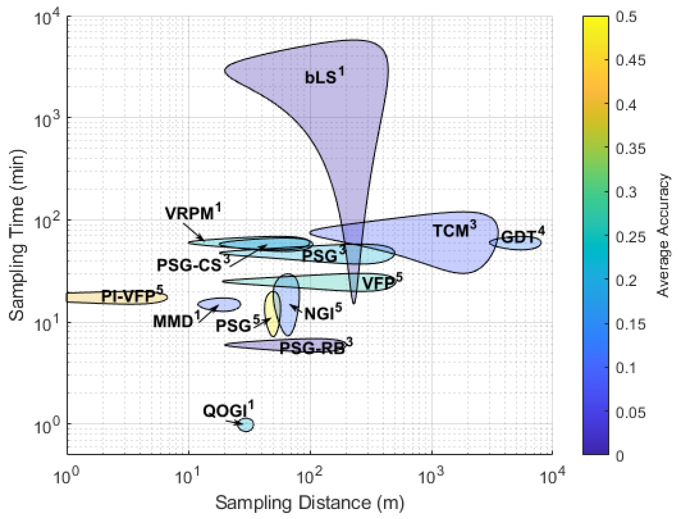
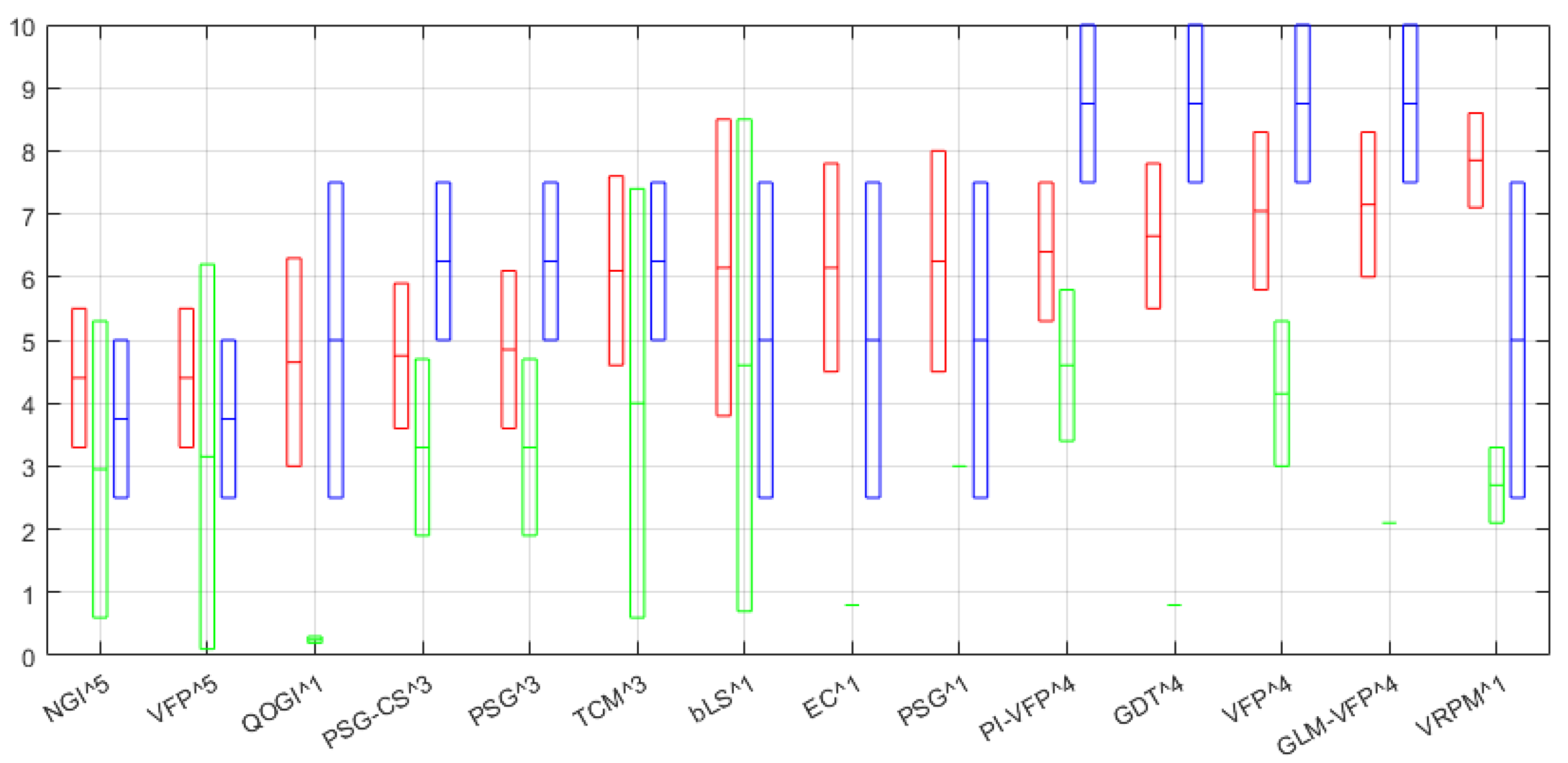
| Method | Assumptions | Sample Distance | Survey Time | Complexity (1–10) | Avg Precision | Avg Accuracy | Avg Cost |
|---|---|---|---|---|---|---|---|
| bLS | x, horizontally uniform surface source atmosphere in horizontal equilibrium | 20–441 m | 15 min–4 days | 3.8–8.5 | ±0.16–0.36 (±0.07–0.85) | ±0.02–0.30 | $–$$$ |
| PSG | x, steady state source rate, point source, plume evolution via ground-level Gaussian dispersion with no obstructions | 441 m 18–500 m 50 m | 4 days 37–58 min 7.22–20 min | 4.5–8 3.6–6.1 3.3–5.5 | (±0.30) , ±0.20–0.67 (±0.19–0.47) ±0.31 | ±0.0022–0.43 ±0.50 | $$–$$$ |
| PSG-RB | PSG assumptions, vertical eddy diffusivity and wind speed approximated by power law scheme | 20–200 m | 6 min | 3.6–6.4 | — | ±0 | $$–$$$ |
| PSG-CS | PSG assumptions, continuous source emission, constant wind speed, vertical eddy diffusivity and wind speed approximated by power law | 18–106 m | 20 min | 3.6–5.9 | ±0.20–0.67 (±0.19–0.47) | ±0.02–0.26 | $$–$$$ |
| NGI | constant source rate, and linear functions of distance to source, plume not capped by atmospheric temp. inversion in z-direction | 50–82.25 m | 7.35–29.62 min | 3.3–5.5 | ±0.21–0.58 (±0.06–0.53) | ±0.11–0.13 | $–$$ |
| MMD | x | 12–27 m | 15 min | 4.5–8.1 | ±0.06 | ±0.10 | $$$–$$$$ |
| GDT | near to no meandering, steady state source rate | 3–8 km | 1 hr | 5.5–7.8 | ±0.07 (±0.08) | ±0.13 | $$$–$$$$ |
| VFP | GDT assumptions | 4.875–10 km 19.08–510 m | 1.5–4.5 h 20–30 min | 5.8–8.3 3.3–5.5 | (±0.30–0.53) ±0.17–0.0.37 (±0.013–0.62) | ±0.10–0.50 ±0.03–0.50 | $$$–$$$$ $–$$ |
| PI-VFP | GDT assumptions | 3 km 0–6.77 m | 20–30 min 15–20 min | 5.3–7.5 3.3–5.5 | (±0.34–0.58) ±0.82 | ±0.27–52 | $$$–$$$$ $–$$ |
| CFP | GDT assumptions | 3–17.84 km | 1 h | 5.5–7.8 | — | — | $$$–$$$$ |
| GLM-VFP | GDT assumptions | 0.4–2.2 km | 2.5 h | 6–8.3 | (±0.21) | — | $$$–$$$ |
| VRPM | GDT assumptions | 10–100 m | 1 h | 7.1–8.6 | ±0.18–0.21 (±0.21–0.33) | ±0.05–0.43 | $–$$$ |
| QOGI | temperature and pressure of gas at leak location are the same, gas plume length in direction of optical path is small | 30 m | 1 min | 3–6.3 | ±0.01–0.02 (±0.02–0.03) | ±0.20–0.24 | $–$$$ |
| TCM | leak plume and tracer plume are well mixed | 100–3546 m | 0.5–2 h | 4.6–7.6 | ±0.06–0.24 (±0.06–0.74) | ±0.0056–0.17 | $$–$$$ |
| EC | stationarity, fully developed turbulent conditions | 25–228 m | — | 4.5–7.8 | (±0.08) | — | $–$$$ |
| Method | Application | Advantages | Disadvantages |
|---|---|---|---|
| bLS | General, Oil and Gas, Agriculture | Able to quantify area source and point source emissions | Sensor is fixed, multiple measurements, negatively impacted by obstacles |
| PSG | Biogas, Oil and Gas | No tracer required | Negatively impacted by obstacles and low wind speeds due to plume advection, mobile sensors limited to roads |
| PSG-RB | Oil and Gas | No tracer required, accurate source quantification in open environments | PSG limitations |
| PSG-CS | Oil and Gas | No tracer required | PSG limitations |
| NGI | General, Oil and Gas | Assumes near-field plume turbulence and wind meandering, No assumption of atmospheric stability class | Near-field ( 100 m), prop-wash interference if unaccounted for |
| MMD | Agriculture | Able to give instantaneous flux estimates | Fixed sensors |
| GDT | Regional | Capable of giving emission quantifications of large areas | Sample around closed volume typically large areas, unable to capture instantaneous methane flux |
| VFP | General, Oil and Gas, Landfill | Does not require exact source location, ease of mobility | Stable atmospheric conditions, unable to capture instantaneous methane flux |
| PI-VFP | General, Oil and Gas | VFP advantages | VFP limitations |
| CFP | General, Urban | Capable of giving emission quantifications of large areas | GDT limitations |
| GLM-VFP | Landfill | VFP advantages | VFP limitations |
| VRPM | Landfill | Able to give instantaneous flux estimates | Fixed sensors |
| QOGI | Biogas | Able to give instantaneous flux estimates | Gas velocity determined via gas camera–velocity component parallel to image plane, can be difficult to process images |
| TCM | General, Oil and Gas, Landfill, Urban | Does not rely on meteorological measurements | Mobile sensors limited to roads, application difficulty due to outside methane source interference |
| EC | General, Oil and Gas | Can capture emission variations due to long time series | Fixed sensor(s), stable atmospheric conditions, sensitive to time of day, typically requires long sampling times |
Publisher’s Note: MDPI stays neutral with regard to jurisdictional claims in published maps and institutional affiliations. |
© 2021 by the authors. Licensee MDPI, Basel, Switzerland. This article is an open access article distributed under the terms and conditions of the Creative Commons Attribution (CC BY) license (https://creativecommons.org/licenses/by/4.0/).
Share and Cite
Hollenbeck, D.; Zulevic, D.; Chen, Y. Advanced Leak Detection and Quantification of Methane Emissions Using sUAS. Drones 2021, 5, 117. https://doi.org/10.3390/drones5040117
Hollenbeck D, Zulevic D, Chen Y. Advanced Leak Detection and Quantification of Methane Emissions Using sUAS. Drones. 2021; 5(4):117. https://doi.org/10.3390/drones5040117
Chicago/Turabian StyleHollenbeck, Derek, Demitrius Zulevic, and Yangquan Chen. 2021. "Advanced Leak Detection and Quantification of Methane Emissions Using sUAS" Drones 5, no. 4: 117. https://doi.org/10.3390/drones5040117
APA StyleHollenbeck, D., Zulevic, D., & Chen, Y. (2021). Advanced Leak Detection and Quantification of Methane Emissions Using sUAS. Drones, 5(4), 117. https://doi.org/10.3390/drones5040117