Classification of Photogrammetric and Airborne LiDAR Point Clouds Using Machine Learning Algorithms

Abstract

With the development of photogrammetry technologies, point clouds have found a wide range of use in academic and commercial areas. This situation has made it essential to extract information from point clouds. In particular, artificial intelligence applications have been used to extract information from point clouds to complex structures. Point cloud classification is also one of the leading areas where these applications are used. In this study, the classification of point clouds obtained by aerial photogrammetry and Light Detection and Ranging (LiDAR) technology belonging to the same region is performed by using machine learning. For this purpose, nine popular machine learning methods have been used. Geometric features obtained from point clouds were used for the feature spaces created for classification. Color information is also added to these in the photogrammetric point cloud. According to the LiDAR point cloud results, the highest overall accuracies were obtained as 0.96 with the Multilayer Perceptron (MLP) method. The lowest overall accuracies were obtained as 0.50 with the AdaBoost method. The method with the highest overall accuracy was achieved with the MLP (0.90) method. The lowest overall accuracy method is the GNB method with 0.25 overall accuracy.

1. Introduction

Extraction of information from three-dimensional (3D) data has become a popular research area in photogrammetry, remote sensing, computer vision and robotics. Classification is defined as the grouping of points under a meaningful cluster by evaluating the particular properties. Classification of point clouds is a challenging field of study, due to their complex structure. In remote sensing, photogrammetric methods, Light Detection and Ranging (LiDAR) systems, Red Green Blue Depth (RGB-D) cameras and Synthetic Aperture Radar (SAR) are methods used to obtain point clouds [1,2]. Point clouds provide rich geometric information for land use land cover applications [3,4] due to their 3D structure.

Machine learning is defined as a mathematical tool for classification of the complex content of point clouds, as in 2D optical images. In machine learning algorithms, classification rules are learned automatically using training data, rather than defined as parameters based on predetermined rules and strong assumptions. Much of the challenging design in a rule-based classification technique is avoided due to automatic feature selection in machine learning. Therefore, machine learning methods are more appropriate than traditional classification methods for complex point cloud data [5].

Many studies have been published in the literature on the use of geometric features for point cloud classification. Weinmann et al. [6] published a comprehensive study on using different geometric features for point cloud classification, choosing the most appropriate neighbourhood and different classifiers. Among these features, the features that positively affect the accuracy have been selected using specific feature selection methods. Oakland 3D Point Cloud Dataset [7], comprising mobile laser scanning data, and Paris-rue-Lille Database [8], which uses the same type of data, were used as the data set. In the study conducted by Vosselman et al. [9], 19 geometric feature features were used. Vaihingen and Rotterdam datasets of the International Society for Photogrammetry and Remote Sensing were used as the dataset. The classification method is Conditional Random Field. As a result of the study, group-based classification has higher accuracy than point-based classification. Guo et al. [5] proposed an ensemble learning method known as JointBoost; ensemble learning methods create a robust classifier by combining multiple weak classifiers. In the first step of the classification, classification is made with the JointBoost method. In the second step, unreliable or mis-classified points are reclassified by using the K-Nearest Neighbour method. Thus, an improvement was achieved as a result of the classification. In the study published by Cabo et al. [10], controlled classification was applied in forest and residential areas. In the study, five geometric features were used from the point cloud: linearity, flatness, sphericity, horizontality and height change. Some popular supervised classification algorithms were used, such as Support Vector Machines (SVM), Random Forest (RF), Logistic Regression, and linear discriminant analysis. In another study published by Becker et al. [11], a controlled classification of point clouds was applied using geometric features. In the study, besides the 15 geometric properties, the color information of the points is added to the feature space, while RF and Gradient Increment Trees were selected as the classifier algorithm. The classes targeted as a result of the classification are ground, higher plants, roads, cars, buildings and manmade objects in a photogrammetric point cloud. In the study conducted by Lin et al. [12], the aerial point cloud was classified by using SVM according to three geometric features: linearity, flatness, and sphericity. The proposed method aimed at increasing the classification accuracy by weighting the covariance matrix used in the calculation, and the targeted classes are divided into buildings and outdoor structures. In the study of Chen et al. [13], both spectral information and 3D spatial information of LiDAR data were used. In the study, a two-stage classification process was carried out to remove noise that reduces classification accuracy. In the first stage, classification based on spectral information was applied using spectral reflection or vegetation index. In the second stage, classification based on spatial data was carried out using the K-Nearest Neighbors (K-NN) algorithm. Atik et al. [14] published a comprehensive study on the performance of eight supervised machine learning methods using geometric features. In the study, the effect of the support area obtained in different scales on the classification accuracy was examined. Moreover, the importance of geometric features was examined according to the data and scale. Dublin City, Oakland3D and Vaihingen data sets obtained with LiDAR were used in the study. Reymann et al. [15] evaluated how multiple echo and intensity information in datasets obtained by LiDAR technology can improve scene classification performance. The density information of the LiDAR data was interpreted, and geometric features were obtained by using Euclidean distances. In addition, a supervised classification process was performed with the Random Forest algorithm by using the density feature and multi-eco features. In the study published by Atik and Duran [16], photogrammetric point cloud classification was made with the popular recurrent neural network algorithms LSTM and BiLSTM, and was carried out on a new photogrammetric dataset proposed in the study. In the classification, not only geometric features but also color information was used; thus, the effect of color information was also examined. The F-1 score building, low vegetation, high vegetation and ground was obtained as 0.85, 0.91, 0.67 and 0.86, respectively.

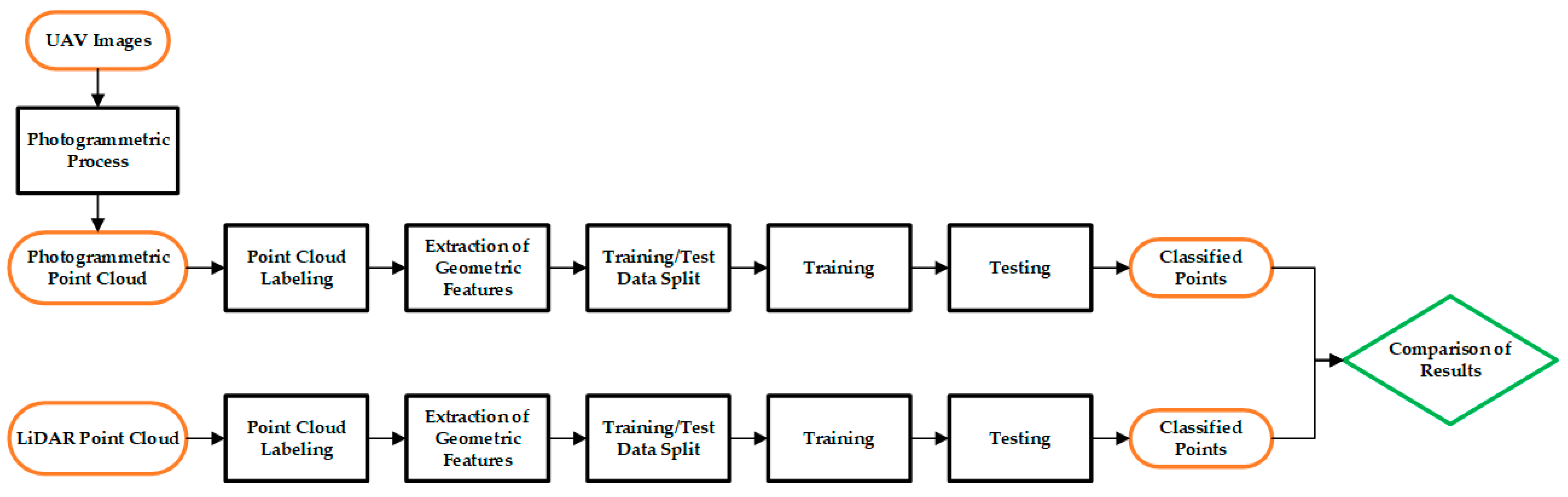
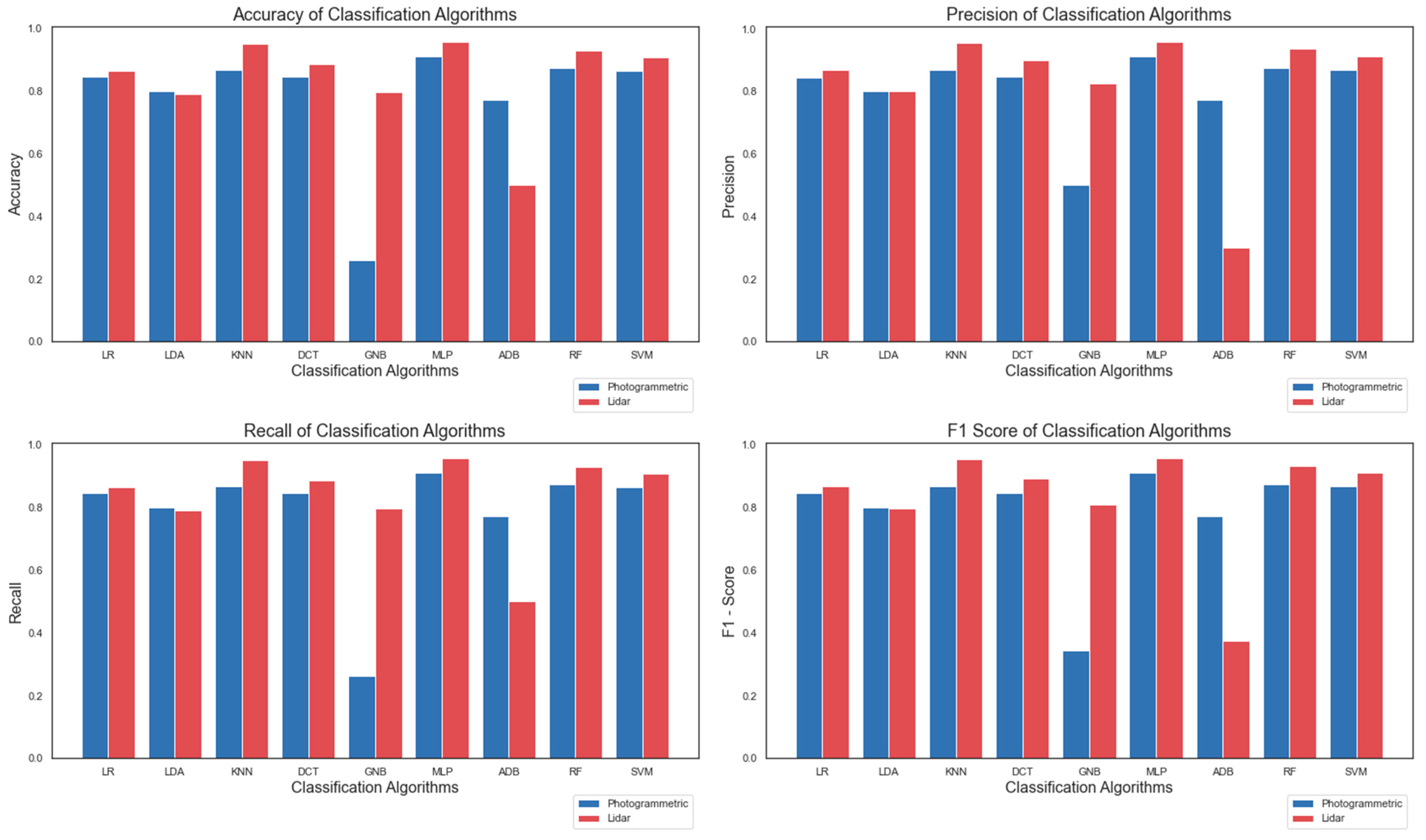
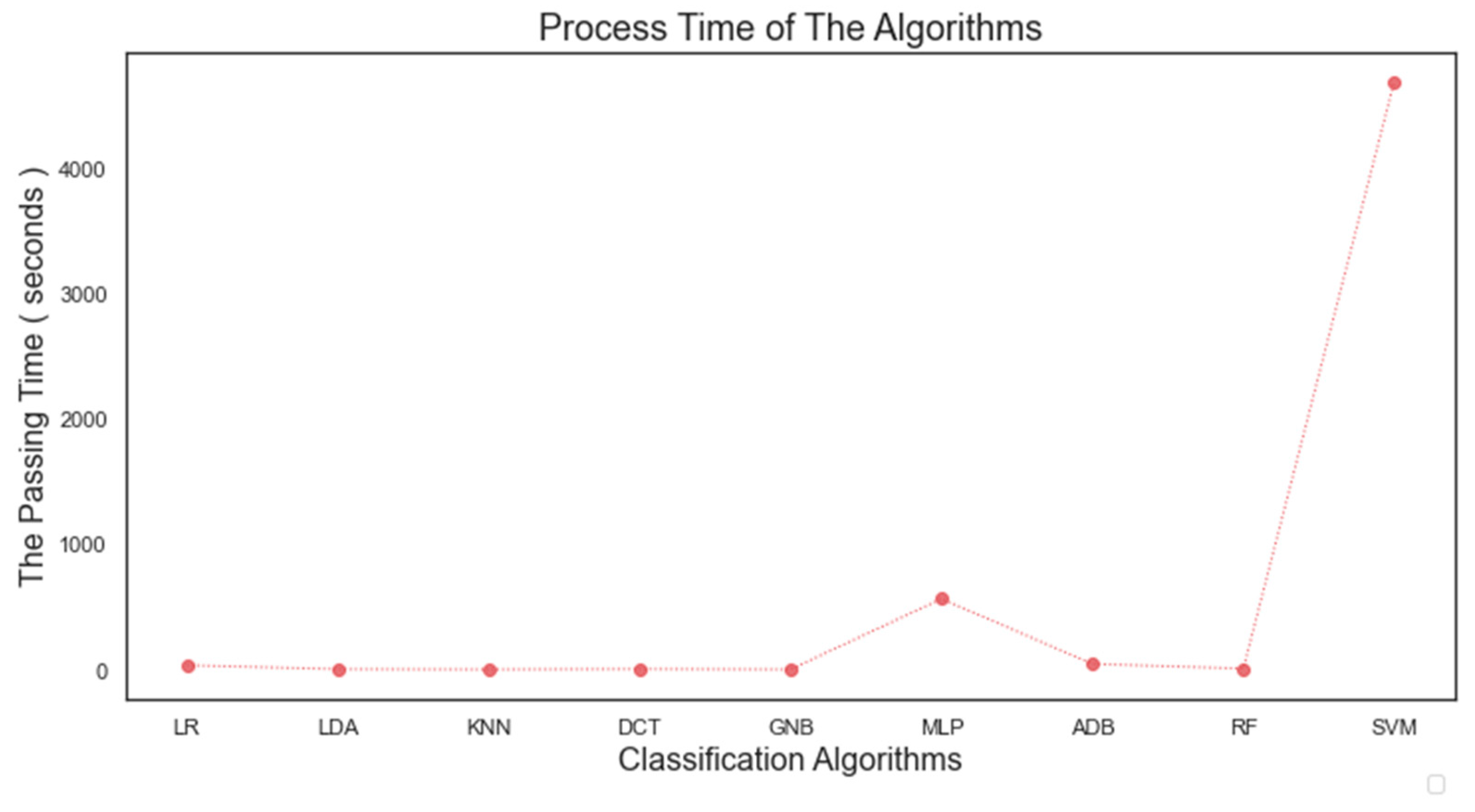
In this study, point clouds obtained from two different sensors (UAV camera and LiDAR) belonging to the same region were classified by different machine learning methods. Thus, it was possible to compare the classification results of point clouds under the same conditions. In this aspect, the study fills an existing gap in the literature. Nine machine learning algorithms were applied for classification purposes: Logistic Regression (LR), linear discriminant analysis (LDA), K-Nearest Neighbors (K-NN), decision tree (DTC), gaussian Naïve Bayes (GNB), Multilayer Perceptron (MLP), AdaBoost (ADB), Random Forest (RF) and Support Vector Machines (SVM). A total of 22 geometric features of the point clouds were calculated and the feature spaces of the points were formed. In the photogrammetric point cloud, color information is also included in the feature space. Random points belonging to different classes selected from the study area were used as training and test data. The points chosen from the point cloud are divided into four classes as building, ground, high vegetation and low vegetation. The usage of geometric features in the classification of point clouds obtained from different sensors has been investigated.

2. Materials and Methods

2.1. Study Area and Data

Istanbul Technical University, Ayazaga Campus, was chosen as the study area. Ayazaga Campus is a campus in Maslak, Istanbul, covering an area of 1,600,000 square meters (Figure 1). The campus includes many different buildings across wooded and grassy areas. The 3D point cloud model of the campus was obtained with an aerial laser scanning system. The accuracy of LiDAR was calculated with 23 ground control points (see Section 2.2. Photogrammetric Process). The horizontal and vertical accuracy of the LiDAR data are about ±8 cm. The average point density of the data is 16 points/m² (Figure 2a). Furthermore, 100,000 points were selected for each class from the objects determined in the LiDAR point cloud. Training and testing were applied with these points.

In this study, DJI Phantom 4 Pro UAV platform is used to capture the high-resolution images in Istanbul Technical University Ayazaga Campus. The camera captures a 5472 × 3648 pixels image size with a horizontal field of view (FOV) of 84 degrees, while the image has three visible (RGB) bands. The camera has 20 μm of pixel size and 8.8 mm of the focal length of the lenses. Flight planning was created with Pix4Dcapture mobile phone application. The flight parameters were determined as forward overlap 80% and side overlaps of 70% and flown at the height of 80 m above. Therefore, Ground Sampling Distance (GSD) is around 3 cm. A total of 3.367 aerial photographs were obtained. Selected points from both LiDAR and photogrammetric point cloud were manually labeled. The data distribution is given in

Table 1. Point distribution of the classes in the datasets.

Class	LiDAR	Photogrammetric
Building	100,000	100,000
High vegetation	100,000	100,000
Low vegetation	100,000	100,000
Ground	100,000	100,000
Total	400,000	400,000

.

2.2. Photogrammetric Data Processing

Photogrammetry deals with 3D reconstruction of objects from images and provides accurate sensor calibration and object modeling using analog or digital images [17]. The point cloud was modeled using Agisoft Photoscan software. The software works depending on the Structure-from-Motion (SfM) algorithm; SfM operates under the basic principles of photogrammetry, that is, the 3D coordinates of an object are calculated by measuring the corresponding points between two overlapping images (Figure 3). Unlike traditional photogrammetry, SFM automatically resolves camera positions and orientation to create object geometry without the need for a target network with predetermined 3D positions. Camera pose and scene geometry are recreated simultaneously by automatically mapping points in multiple images, while camera positions and object coordinates can be estimated with the coordinates of these points obtained in each image. The initial estimated values are then iteratively improved using non-linear least squares adjustment [18]. For this, at least two photographs of the same object are used [19].

In terms of alignment photographs, 3.367 aerial photos were aligned using automatically detected features from each image via the software. Ground control points were then marked for a coordinated and scaled model. The photogrammetric point cloud georeferencing was carried out using 23 ground control points (GCP) whose XYZ coordinates were measured by terrestrial measurements (using Global Navigation Satellite System (GNSS)). The horizontal accuracy of the point cloud was 9.3 cm, and the vertical accuracy was 5.2 cm. After the images were aligned to each other, the dense point cloud was obtained (Figure 2b). The point cloud density is 83 pts/m² and the spatial resolution is approximately 9 cm. 100,000 points were randomly selected from each determined class. In total, 400,000 from the point cloud obtained by aerial photogrammetry for training and testing. The data acquisition time is approximately 5 h and the processing time is 10 h.

2.3. Classification Methods

2.3.1. Logistic Regression (LR)

Logistic regression (LR) [20] is a probabilistic statistical classification algorithm. Logistic regression applies a linear transformation is applied between the input variables and the probabilities of the output variable. Relational hypotheses between a categorical output variable and one or more categorical variables can be explained and tested with LR [21]. As a result, the probability of observation for a category is obtained. The mathematical model of the LR classifier is given in Equation (1)

$$\ln \frac{P\left(Y=i\right)}{P\left(Y=C\right)}={\alpha }_i+{\displaystyle \sum }_{j=1}^p{\beta }_j{x}_{j }$$

(1)

where Y is the output variable, α_i and β_j are the coefficients of the model, and x₁, x₂, …, x_p are the covariates. Logit, which is the natural logarithm of a probability ratio, is the basic mathematical concept of the LR. If we consider a bivariate classification, the natural logarithm of the ratio of the case i of class Y and the case C that is equal to 1 − i, gives the logit of the case i. This natural logarithm value is used as the regression coefficient of the Logistic Regression classifier. Data are assigned to a class of the maximum probability:

$$P\left(Y=i|X\right)=\frac{e^{{\alpha }_i+{{\displaystyle \sum }}_{i=1}^{j=p}{\beta }_j{X}_j}}{1+e^{{\alpha }_i+{{\displaystyle \sum }}_{i=1}^{j=p}{\beta }_j{X}_j}}$$

(2)

2.3.2. Linear Discriminant Analysis (LDA)

Linear Discriminant Analysis (LDA) [22] is a linear transformation aimed at calculating the directions of the axes that best separate multiple classes. If a vector is defined as w, all data is projected onto this vector:

$$z={\mathit{w}}^t\mathit{x}$$

(3)

where z is the projection of data (x) onto w and t indicates the vector transposition. In order to separate the classes well after the projection, the average of the samples in each class should be kept as far from each other as possible and the class samples should be distributed to a small area as possible. It is ensured that the within-class (S_i) (Equation (4)) and between-class (S_B) (Equation (5)) distribution matrices (R = S_i/S_B) have the maximum ratio.

$$S_i={\displaystyle \sum }_t{r}_i^t\left({\mathit{x}}^t-{\mathit{m}}_i\right){\left({\mathit{x}}^t-{\mathit{m}}_i\right)}^t$$

(4)

$$S_B={\displaystyle \sum }_{i=1}^K{N}_i\left({\mathit{m}}_i-\mathit{m}\right){\left({\mathit{m}}_i-\mathit{m}\right)}^t$$

(5)

where m_i is the means of samples from class i and m is the sum of m_i. The algorithm assigns elements to each class by maximizing R. The problem is solved with the largest eigenvectors $S_W^{-1}{S}_B$, where S_w is the sum of the within-class distribution matrix. According to LDA, attributes (input or explanatory variables) are distributed continuously and normally, and the dependent output variable is categorical [10].

2.3.3. K-Nearest Neighbors (K-NN)

K-Nearest Neighbors (K-NN) classifier is an example-based learning type because a data-dependent internal model is not developed. [23]. The K-NN, which is a nonparametric method, is not limited to a fixed number of parameters. Since K-NN does not have initial parameters, it creates and applies a function based on training data. K-NN is advantageous over other methods as it can explain the result of the classification of neighbours.

For each data in the X input data set, the closest neighbouring points are found. Neighbouring points are weighted in inverse proportion to the Euclidean distance between them and the query point. The majority class in the neighbourhood area is assigned as the class of the input x. In application of the K-NN method, K is usually taken as a single number to minimize confusion between classes because confusion generally occurs between two neighbouring classes.

2.3.4. Decision Tree Classifier (DTC)

The decision tree is an algorithm that calculates parameters for each part by dividing the input space into subparts. Decision tree is a nonparametric classification and regression algorithm. It consists of nodes that divide each part of the decision tree into subparts. If there is a decision tree of undetermined size, the algorithm can be thought of as nonparametric [24]. The decision tree also has some disadvantages. In some cases, it can create complex decision trees. Decision trees can be unstable as small changes in the data are affected. However, it is preferred due to its ease of calculation.

2.3.5. Naïve Bayes (NB)

The basic logic of Naïve Bayes classifier works by calculating a separator function for each class and assigning an example to the class in which the function gets the maximum value [25]. f_i(E) indicates the discriminant function corresponding to the i^th class. The discriminant function for a feature vector a can be written as:

$$f_i\left(E\right)=P\left(C_i\right){\displaystyle \prod }_{j=1}^{a}P\left(A_j=v_{jk}|C_i\right)$$

(6)

where A_j is a feature and v_jk is the value of the feature A_j. The classifier that estimates the relevant probabilities in the training set using this discriminant function is often called the Naïve Bayes classifier [26]. NB classifier is defined as a probabilistic method based on Bayes’ theorem that studies the probability relationship between a given data point x and class C. (Equation (7)) [27].

$$P\left(C|\mathrm{x}\right)=\frac{P\left(x|C\right)}{P\left(x\right)}$$

(7)

Gauss Naïve Bayes (GNB), the most used Naïve Bayes classifier, applies the classification assuming the probability of the properties to be Gaussian [28]. The formulation is as in Equation (8):

$$P\left(x_{ i}|C\right)=\frac{1}{\sqrt{2\pi {\sigma }_C^2}}\exp \left(-\frac{{\left(x_i-{\mu }_C\right)}^2}{2{\sigma }_C^2}\right)$$

(8)

2.3.6. Multilayer Perceptron (MLP)

Multilayer Perceptron (MLP) is a supervised learning method that learns a function by training on a dataset. Multilayer Perceptron can be used to solve non-linear classification problems [28]. Thus, it differs from Logistic Regression [29]. In the MLP, there is a forward and backward propagation between layers. While calculating the output and error value of the network in the forward propagation phase, the connection weight values are updated to minimize the error value in the back-propagation phase.

The value x is given to the input layer. “Activation” moves forward and z_h values are calculated in hidden layers. Hidden layer units, each of them a detector, apply the non-linear sigmoid function to weighted sum:

$$z_h=\mathrm{sigmoid}\left(w_h^{T}x\right)=\frac{1}{1+\exp \left[-({{\displaystyle \sum }}_j^d{w}_{hj}{x}_j+w_{h0})\right]}$$

(9)

The sensors in this section calculate y_i values in the output layer using the calculated values in hidden layers as input values. [28].

$$y_i={\mathit{v}}_i^t\mathit{z}={\displaystyle \sum }_{h=1}^H{v}_{ih}{z}_h+v_{i0 }$$

(10)

where z_h is the bias weights in the hidden layer and v_i0 is the bias weights. v_ih are the weights in the second layer. Although there is no non-linearity in the outputs of the y calculation in regression problems, the results of the discriminant functions are non-linear when K > 2 (K is the number of classes).

2.3.7. Adaboost (ADB)

Boosting methods combine weak classifiers to create a robust classifier. In boosting, complementary basic classifiers are actively created by training the next classifier about the errors of the previous classifiers [28].

AdaBoost is a machine learning meta-algorithm formulated by Freund and Schapire [30]. AdaBoost is used effectively with weak classifiers. The most convenient and common algorithm used with AdaBoost is single-level decision trees. These trees are often called decision logs because they are so short and only contain a decision for classification. Each example in the training dataset is weighted (Equation (11)).

$$weight\left(x_i\right)=\frac{1}{n}$$

(11)

x_i represents each part of the data in the training set, and n is the total number of data. For training purposes, weak classifiers are added separately and trained with weighted training data. The process continues until a predetermined number of weak classifiers (user parameters) are created or no further improvements can be made in the training dataset. The estimates are made by calculating the weighted average of the weak classifiers.

2.3.8. Random Forest (RF)

Random Forest [31] is an advanced version of bagging that creates and averages individual trees. Each tree in the Random Forest gives a class prediction, and the highest-scoring class is assigned as the model’s prediction. RF allows random sampling of each tree from the dataset through a modification process known as bagging. Bagging increases accuracy when using random features and determines generalized error (PE*) estimates of the community. RF classifier needs two basic parameters: the number of variables used in each node and the number of trees to be developed to determine the best split. As a result of these operations, a generalized error is obtained. The generalized error calculation is shown in Equation (12).

$$P{E}^{*}=P_{X,Y}\left(mg\left(X,Y\right)<0\right)$$

(12)

where mg() is the margin function. Margin measures the difference in the average number of votes in (X, Y) for the correct class from the average number of votes for any other class. The size of the margin value indicates the reliability of the classification [12].

2.3.9. Support Vector Machines (SVM)

Support Vector Machines (SVM) [32] is a popular supervised machine learning algorithm used in classification or regression. SVM aims to find a plane that has the maximum distance between data points of two classes. The distance is called the maximum margin. Maximizing the margin distance allows the data points to be classified as more secure.

In addition to linear classification, SVMs can perform a non-linear classification using functions called kernel tricks by indirectly mapping their inputs to high-dimensional feature fields. Linear boundaries in the extended field provide better class separation and become non-linear boundaries with kernel tricks. Nonlinearly separable input data is displayed in a high-dimensional feature space. Extending to more complex decision surfaces works by mapping the input variable x to a higher dimensional property area and making linear classification in that area. Input variable x maps to a vector of the new property space (Equation (13)).

$$x\to \varnothing \left(x\right)=(a_1\varnothing \left(x\right),a_2{\varnothing }_2\left(x\right),\dots ,a_n{\varnothing }_n\left(x\right))$$

(13)

The solution of a two-class problem with the kernel trick can be mathematically expressed as;

$$f\left(x\right)=sign\left({\displaystyle \sum }_i{\lambda }_i{y}_i\varnothing \left(x\right).\varnothing \left(x_i\right)+b\right)$$

(14)

where λ_i are the non-negative Lagrange multiplier, y_i denotes the class of the input data and b is the parameter of the hyper-plane.

2.4. Geometric Features

Geometric features are widely used to describe the local geometry of LiDAR points. These features determine the geometric relationship of a point to points in a given area around it. Depending on a specified scale, these geometric features can be determined. Geometric features of any point p of the point cloud are obtained by using the eigenvalues (λ₁, λ₂, λ₃) of the eigenvectors (v₁, v₂, v₃) derived from the covariance matrix:

$$cov\left(\mathrm{S}\right)=\frac{1}{S}{\displaystyle \sum }_{p\in S}\left(\mathit{p}-\overline{\mathit{p}} \right){\left(\mathit{p}-\overline{\mathit{p}} \right)}^t$$

(15)

where $\overline{\mathit{p}}$ is the centroid of the support S. In this study, many values are calculated as geometric features such as roughness, curvatures (mean, gaussian, normal change rate), number of neighbours, surface density, volume density, 1st order moment, the sum of eigenvalues, omnivariance, eigenentropy, anisotropy, planarity, linearity, surface variation, sphericity, verticality, PCA1, PCA2, eigenvalues (λ₁, λ₂, λ₃) (

Table 2. Geometric features used in the study.

Feature	Explanation	Feature	Explanation
1st eigenvalue	${\lambda }_1$	PCA1	${\lambda }_1/\left({\lambda }_1+{\lambda }_2+{\lambda }_3\right)$
2st eigenvalues	${\lambda }_2$	PCA2	${\lambda }_2/\left({\lambda }_1+{\lambda }_2+{\lambda }_3\right)$
3st eigenvalue	${\lambda }_3$	Height value	Zi
Sum of eigenvalues	${\lambda }_1+{\lambda }_2+{\lambda }_3$	Surface density	Number of neighbour/neighbourhood area
Anisotropy	$({\lambda }_1-{\lambda }_3)/{\lambda }_1$	Volume density	Number of neighbour/neighbourhood volume
Planarity	$({\lambda }_2-{\lambda }_3)/{\lambda }_1$	Number of neighbours	Other features
Linearity	$({\lambda }_1-{\lambda }_2)/{\lambda }_1$	1st order moment
Surface variation	${\lambda }_3/\left({\lambda }_1+{\lambda }_2+{\lambda }_3\right)$	Roughness
Sphericity	${\lambda }_3/{\lambda }_1$	Mean curvature
Verticality	$1-|\langle \left[0 0 1\right],{\lambda }_3\rangle |$	Gaussian curvature
		Normal change rate

). Optimum radius was selected because geometric features are calculated depending on the support area [6]. The feature computation time is 240 s and 15 s for photogrammetric point cloud and LiDAR point cloud, respectively.

2.5. Experiment

Cloud Compare, open-source software, was used for calculating 22 geometric features for both the LiDAR point cloud and the photogrammetric point cloud. The support area is an important parameter in calculating geometric features. Support area refers to the area in which neighbour points of a point are determined. In this study, 0.5 m within the LiDAR point cloud and 0.05 m for the photogrammetric point cloud were experimentally determined as the optimum support radius. The workflow of the study is presented in Figure 4.

Due to the size of the point clouds, it was not possible to use all points as inputs in machine learning algorithms. For this reason, random selection was made from the data sets, with the same number of items in each class. Thus, errors arising from unbalanced data distribution in classes are prevented. The same number of random and homogeneously distributed point selection procedures was performed for the four classes defined (surface, dense woodland, green area, and structure). 100,000 points were chosen from each class. Random 1/3 test data was selected from this prepared data set. Other points are separated as training data set. In the study, point clouds were classified using nine machine learning algorithms: LR, LDA, K-NN, DTC, GNB, MLP, ADB, RF, SVM. The algorithms were trained using training data. The optimum values of the parameters of the algorithms were determined experimentally (see Section 4). Algorithms were developed and implemented through the Python programming language. Scikit-learn, a popular library developed in the Python language, was used.

Overall Accuracy is metric that measures the proportion of points correctly classified. Metric values obtained in machine learning are calculated with a confusion matrix. The equations of the metrics are shown in Equations (16)–(19).

$$Overall Accuracy=\frac{TP+TN}{TP+TN+FP+TN}$$

(16)

$$Precision=\frac{TP}{TP+FP}$$

(17)

$$Recall=\frac{TP}{TP+FN}$$

(18)

$$F1 score=2\frac{Precision · Recall}{Precision+Recall}$$

(19)

True positive (TP) is the number of points that are predicted to be labeled as positive and the actual label is positive. True negative (TN) is the number of points that are predicted to be labeled as negative and the actual label is negative. False positive (FP) is defined as the number of points that are predicted to be labeled as positive, but the actual label is negative. False negative (FN) is defined as the number of points that are predicted to be labeled as negative, but the actual label is positive [33]. These metrics allow us to pinpoint what types of misclassifications occur. Thus, it is possible to detect more accurately the situations that cause errors in the classification.

3. Results

Machine learning algorithms have been applied to the LiDAR dataset and the photogrammetric point cloud dataset. Thus, the performance of machine learning algorithms in the classification of point clouds obtained by different methods was examined. Overall accuracy, precision, recall and F1 score were calculated as classification evaluation metrics of these models. The points in the datasets split training and testing. 70% of the points used for training and 30% of the point was used for testing. A balanced distribution of test and training data was provided for each class.

According to the data obtained from the LiDAR point cloud, the highest overall accuracies were obtained as 0.96 with the MLP method and 0.95 with the K-NN method. The lowest general accuracies were obtained as 0.50 with AdaBoost method. It has been concluded that AdaBoost algorithm gives dramatically lower accuracy compared to other methods. The method with the highest precision, recall and F1 score is again the MLP method with values of 0.96, 0.96 and 0.96, respectively. The method with the lowest precision, recall, F1 score is the AdaBoost method with values of 0.30, 0.50 and 0.38, respectively. The results of the methods in the LiDAR dataset are shown in

Table 3. The results of the LiDAR point cloud for each algorithm. The results were between 0–1.

Algorithm	Accuracy	Precision	Recall	F1 Score	Computation Time (Seconds)
LR	0.87	0.87	0.87	0.87	2.8
LDA	0.79	0.80	0.79	0.80	0.4
K-NN	0.95	0.96	0.95	0.95	1.2
DTC	0.89	0.90	0.89	0.89	0.4
GNB	0.80	0.83	0.80	0.81	0.05
MLP	0.96	0.96	0.96	0.96	135.3
ADB	0.50	0.30	0.50	0.38	3.8
RF	0.91	0.92	0.91	0.92	1.0
SVM	0.91	0.91	0.91	0.91	28.2

.

It is concluded that the results in the photogrammetric point cloud dataset generally show a decrease in the evaluation metrics. The method with the highest general accuracy was achieved with the MLP (0.90) method, as in the LiDAR dataset. The second method with the highest overall accuracy is the Logistic Regression method, with an accuracy of 0.84. The lowest overall accuracy method is the GNB method with 0.25 of overall accuracy. Additionally, compared with the LiDAR dataset, it is observed that there is a very high increase in the AdaBoost method with 0.76 of overall accuracy. The highest precision and recall values were obtained with the MLP method with 0.90 and 0.90, respectively. The lowest precision and recall values were obtained with the GNB method with 0.31 and 0.25, respectively. Similarly, in the F1 score value, the best result was obtained with the MLP method as 0.90, while the lowest value was obtained as 0.28 with the GNB method (

Table 4. The results of the photogrammetric point cloud for each algorithm. The results were between 0–1.

Algorithm	Accuracy	Precision	Recall	F1 Score	Computation Time (Seconds)
LR	0.84	0.84	0.84	0.84	2.8
LDA	0.79	0.79	0.79	0.79	0.4
K-NN	0.83	0.83	0.83	0.83	1.2
DTC	0.79	0.79	0.79	0.79	0.4
GNB	0.25	0.31	0.25	0.28	0.05
MLP	0.90	0.90	0.90	0.90	135.3
ADB	0.76	0.76	0.76	0.76	3.8
RF	0.78	0.81	0.78	0.80	1.0
SVM	0.81	0.83	0.81	0.82	28.2

). In all methods except the AdaBoost method, higher metrics were obtained in the LiDAR point cloud. Comparative results are shown in Figure 5.

The results were also analyzed for each class. The best precision values for the building class in the Lidar dataset were obtained by the MLP and K-NN methods. These two methods detect all buildings as positive. However, the MLP method has the highest recall value of 0.99. According to the F1 score, the building class is determined with the highest accuracy by the MLP method. The AdaBoost method has the lowest metrics for finding the building class. In the AdaBoost method, the building points are generally mixed with the ground points. Therefore, almost no building points have been detected correctly. In the Forest class, the method with the highest accuracy is K-NN with 0.93 and the method with the lowest F1 value is the AdaBoost method with a value of 0.67. Algorithms are more successful in detecting the ground class than other classes. In low vegetation class, RF method (0.94) has the highest precision value, LDA method (0.99) in recall value and K-NN method (0.94) in F1 score (

Table 5. The precision values for each class in LiDAR dataset. The results were between 0–1.

	LR	LDA	K-NN	DTC	GNB	MLP	ADB	RF	SVM
Building	0.88	0.71	1.00	0.94	0.94	1.00	0.2	0.93	0.98
High vegetation	0.92	0.98	0.98	0.74	0.91	0.95	0.5	0.81	0.93
Ground	0.82	0.71	0.95	1.00	0.77	1.00	0.5	1.00	0.87
Low vegetation	0.86	0.81	0.89	0.92	0.69	0.9	0.00	0.94	0.88

,

Table 6. The recall values for each class in LiDAR dataset. The results were between 0–1.

	LR	LDA	K-NN	DTC	GNB	MLP	ADB	RF	SVM
Building	0.8	0.71	0.95	1.00	0.69	0.99	0.00	0.93	0.84
High vegetation	0.85	0.76	0.88	0.94	0.57	0.89	1.00	0.81	0.87
Ground	0.88	0.71	1.00	0.94	0.97	1.00	1.00	1.00	0.98
Low vegetation	0.93	0.99	0.98	0.67	0.96	0.95	0.00	0.94	0.94

,

Table 7. The F1-score values for each class in LiDAR dataset. The results were between 0–1.

	LR	LDA	K-NN	DTC	GNB	MLP	ADB	RF	SVM
Building	0.84	0.71	0.97	0.97	0.8	0.99	0.00	0.96	0.9
High vegetation	0.88	0.86	0.93	0.83	0.7	0.92	0.67	0.87	0.9
Ground	0.85	0.71	0.98	0.97	0.86	1.00	0.67	1.00	0.92
Low vegetation	0.89	0.89	0.94	0.77	0.81	0.92	0.00	0.85	0.91

,

Table 8. The precision values for each class in the photogrammetric point cloud. The results were between 0–1.

	LR	LDA	K-NN	DTC	GNB	MLP	ADB	RF	SVM
Building	0.77	0.67	0.78	0.70	1.00	0.87	0.63	0.61	0.65
High vegetation	0.85	0.80	0.77	0.80	0.00	0.93	0.71	0.83	0.85
Ground	0.82	0.81	0.84	0.86	0.25	0.85	0.84	0.94	0.86
Low vegetation	0.91	0.89	0.91	0.82	0.00	0.94	0.88	0.87	0.94

,

Table 9. The recall values for each class in the photogrammetric point cloud. The results were between 0–1.

	LR	LDA	K-NN	DTC	GNB	MLP	ADB	RF	SVM
Building	0.74	0.68	0.68	0.76	0.00	0.81	0.64	0.86	0.82
High vegetation	0.82	0.79	0.84	0.70	0.00	0.90	0.74	0.72	0.79
Ground	0.87	0.80	0.89	0.80	1.00	0.93	0.83	0.65	0.78
Low vegetation	0.93	0.91	0.89	0.89	0.00	0.95	0.84	0.91	0.86

and

Table 10. The F1 score values for each class in the photogrammetric point cloud. The results were between 0–1.

	LR	LDA	K-NN	DTC	GNB	MLP	ADB	RF	SVM
Building	0.75	0.68	0.73	0.73	0.00	0.84	0.63	0.72	0.73
High vegetation	0.84	0.79	0.80	0.75	0.00	0.91	0.72	0.77	0.82
Ground	0.85	0.80	0.87	0.83	0.40	0.89	0.84	0.77	0.82
Low vegetation	0.92	0.90	0.90	0.85	0.00	0.95	0.86	0.89	0.89

).

In both data sets, the duration of the algorithms during the classification is recorded in seconds. While the algorithm that produces the fastest results in the data set obtained from LIDAR technology is the K-Nearest Neighbours (K-NN) algorithm, the algorithm that produces results in the longest time is the Support Vector Machine (SVM) algorithm. In the data set obtained from air photogrammetry, the algorithm that produces the fastest results is the K-NN algorithm, as in LIDAR, and the algorithm with the longest duration is the SVM algorithm (Figure 6).

4. Discussion

The performances of machine learning algorithms on LiDAR and photogrammetric point clouds were compared. Generally, algorithms appear to have higher metrics in the LiDAR point cloud. Geometric features are calculated more accurately since the number of unrelated points in point support areas is less.

Hyperparameters are parameters that can be optimized during the training process of the model. The selection of the optimum hyperparameters is important because of their impact on the performance of the classification algorithm. In the study, random search method was used for the selection of suitable hyperparameters. This method was first announced in an article published by Bergstra and Bengio (2012) [34]. The method is based on the determination of the hyperparameter range using the prior knowledge of the problem. Then, instead of trying each of the values in this range, random values are selected for finding the most appropriate value for the hyperparameters. In the K-NN method, the appropriate neighbour size was determined by this method. As another hyperparameter example, “Adam” is used for the optimization of the weights in the MLP algorithm. The reason for this is that Adam is a stochastic gradient-based optimizer, which achieves good success on large datasets.

According to the results, it was concluded that the GNB method shows a lower performance in noisy data (Table 8, Table 9 and Table 10). The LiDAR point cloud has a lower density than the photogrammetric point cloud. Since the AdaBoost algorithm is an ensemble method consisting of weak classifiers, it is understood that the geometric features calculated from the support fields in the LiDAR dataset are not distinctive enough for AdaBoost (Table 5, Table 6 and Table 7). MLP method, which is a neural network-based method, has the highest metrics in both datasets. These results are also compatible with previous studies [16]. It is concluded that neural network-based classifiers have the potential for point cloud classification. SVM and MLP methods have a long classification period for real-time applications (Figure 6). K-NN and LR methods can be preferred for real-time applications in terms of time and accuracy balance (Figure 6). All evaluation metrics of GNB method decreased compared to Lidar point cloud results. The results of the methods in the photogrammetric dataset are shown in (Table 4). While MLP and RF are the most accurate methods in the ground class, the lowest accuracy method is the AdaBoost method. When the photogrammetric point cloud is examined, the building class ground class is generally mixed in the GNB method. All of the buildings are labeled as ground. The highest precision, recall and F1 score values were obtained by MLP method. As in the building class, the highest metrics in ground, forest and low vegetation classes were obtained with the MLP method. The method with the lowest metrics is GNB method. Although the value of 1 is obtained in some metrics with the GNB method, this value is not meaningful because very few points are labeled correctly. Class-based metric values of the photogrammetric point cloud are presented in Table 8, Table 9 and Table 10. In this study, an original dataset was created. Users whose machine learning methods are reproducible can repeat the experiment over the shared dataset.

Optimum neighbourhood radius selection is an important factor affecting the classification [14]. If a large neighbourhood radius is chosen to calculate geometric features, the computational load increases considerably and the distinctiveness of the points decreases. If a small neighbourhood radius is chosen, the geometry around the point cannot be defined sufficiently, so the geometric properties are similar at all points. Thus, the neighbourhood value chosen for the photogrammetric point cloud is smaller than that of LiDAR, because the geometry around the point can be defined with fewer points in the photogrammetric point cloud. In order to define the geometric properties of a point correctly in LiDAR, a larger neighbourhood area is required. Most of the methods have higher accuracy in the LiDAR point cloud. K-NN, GNB, RF and SVM methods have high accuracy in LiDAR point cloud that have lower point density (Table 3). ADB, which is a boosting method, has higher accuracy in the photogrammetric point cloud (Table 4).

5. Conclusions

This study examined the performances of nine different machine learning algorithms in the classification of point clouds obtained by LIDAR and aerial photogrammetry. As a result of the point cloud classification process, the building, high vegetation, ground and low vegetation were classified. In the classification process, it has been done by using the geometric features of the data. Thus, the classification process was carried out without additional information other than 3D coordinates of the points.

Machine learning algorithms are used to classify point clouds obtained by different sensors. Machine learning methods have significant potential for the classification of point clouds. This study can be carried out in areas with land use and land cover structure in future studies. In addition to geometric features, the feature spaces can be expanded by using LiDAR point clouds and images together. Among the machine learning methods, especially those based on neural network (such as MLP), have shown successful results. As data complexity increases, neural network-based methods can be used. The results of this study have the potential to be a reference for future studies.

References

1. Geng, X.; Ji, S.; Lu, M.; Zhao, L. Multi-Scale Attentive Aggregation for LiDAR Point Cloud Segmentation. Remote Sens. 2021, 13, 691. [Google Scholar] [CrossRef]
2. Akyol, O.; Duran, Z. Low-cost laser scanning system design. J. Russ. Laser Res. 2014, 35, 244–251. [Google Scholar] [CrossRef]
3. Donmez, S.O.; Ipbuker, C. Investigation on Agent Based Models for Image Classification of Land Use and Land Cover Maps. In Proceedings of the 39th Asian Conference on Remote Sensing (ACRS): Remote Sensing Enabling Prosperity, Kuala Lumpur, Malaysia, 15–19 October 2018; pp. 2005–2008. [Google Scholar]
4. Atik, S.O.; Ipbuker, C. Integrating Convolutional Neural Network and Multiresolution Segmentation for Land Cover and Land Use Mapping Using Satellite Imagery. Appl. Sci. 2021, 11, 5551. [Google Scholar] [CrossRef]
5. Guo, B.; Huang, X.; Zhang, F.; Sohn, G. Classification of airborne laser scanning data using JointBoost. ISPRS J. Photogramm. Remote Sens. 2015, 100, 71–83. [Google Scholar] [CrossRef]
6. Weinmann, M.; Jutzi, B.; Hinz, S.; Mallet, C. Semantic point cloud interpretation based on optimal neighborhoods, relevant features and efficient classifiers. ISPRS J. Photogramm. Remote Sens. 2015, 105, 286–304. [Google Scholar] [CrossRef]
7. Munoz, D.; Bagnell, J.A.; Vandapel, N.; Hebert, M. Contextual classification with functional max-margin markov networks. In Proceedings of the 2009 IEEE Conference on Computer Vision and Pattern Recognition, Miami, FL, USA, 20–25 June 2009; pp. 975–982. [Google Scholar]
8. Serna, A.; Marcotegui, B.; Goulette, F.; Deschaud, J.E. Paris-rue-Madame database: A 3D mobile laser scanner dataset for benchmarking urban detection, segmentation and classification methods. In Proceedings of the 4th International Conference on Pattern Recognition Applications and Methods (ICPRAM 2014), Angers, France, 6–8 March 2014. [Google Scholar]
9. Vosselman, G.; Coenen, M.; Rottensteiner, F. Contextual segment-based classification of airborne laser scanner data. ISPRS J. Photogramm. Remote Sens. 2017, 128, 354–371. [Google Scholar] [CrossRef]
10. Cabo, C.; Ordóñez, C.; Sáchez-Lasheras, F.; Roca-Pardiñas, J.; de Cos-Juez, J. Multiscale Supervised Classification of Point Clouds with Urban and Forest Applications. Sensors 2019, 19, 4523. [Google Scholar] [CrossRef] [Green Version]
11. Becker, C.; Rosinskaya, E.; Häni, N.; d’Angelo, E.; Strecha, C. Classification of aerial photogrammetric 3D point clouds. Photogramm. Eng. Remote Sens. 2018, 84, 287–295. [Google Scholar] [CrossRef]
12. Lin, C.H.; Chen, J.Y.; Su, P.L.; Chen, C.H. Eigen-feature analysis of weighted covariance matrices for LiDAR point cloud classification. ISPRS J. Photogramm. Remote Sens. 2014, 94, 70–79. [Google Scholar] [CrossRef]
13. Chen, B.; Shi, S.; Gong, W.; Zhang, Q.; Yang, J.; Du, L.; Song, S. Multispectral LiDAR point cloud classification: A two-step approach. Remote Sens. 2017, 9, 373. [Google Scholar] [CrossRef] [Green Version]
14. Atik, M.E.; Duran, Z.; Seker, D.Z. Machine Learning-Based Supervised Classification of Point Clouds Using Multiscale Geometric Features. ISPRS Int. J. Geo-Inf. 2021, 10, 187. [Google Scholar] [CrossRef]
15. Reymann, C.; Lacroix, S. Improving LiDAR point cloud classification using intensities and multiple echoes. In Proceedings of the 2015 IEEE/RSJ International Conference on Intelligent Robots and Systems (IROS), Hamburg, Germany, 28 September–2 October 2015; IEEE: Manhattan, NY, USA, 2015; pp. 5122–5128. [Google Scholar]
16. Atik, M.E.; Duran, Z. Classification of Aerial Photogrammetric Point Cloud Using Recurrent Neural Networks. Fresenius Environ. Bull. 2021, 30, 4270–4275. [Google Scholar]
17. Duran, Z.; Aydar, U. Digital modeling of world’s first known length reference unit: The Nippur cubit rod. J. Cult. Herit. 2012, 13, 352–356. [Google Scholar] [CrossRef]
18. Westoby, M.J.; Brasington, J.; Glasser, N.F.; Hambrey, M.J.; Reynolds, J.M. ‘Structure-from-Motion’ photogrammetry: A low-cost, effective tool for geoscience applications. Geomorphology 2012, 179, 300–314. [Google Scholar] [CrossRef] [Green Version]
19. Atik, M.E.; Ozturk, O.; Duran, Z.; Seker, D.Z. An automatic image matching algorithm based on thin plate splines. Earth Sci. Inform. 2020, 13, 869–882. [Google Scholar] [CrossRef]
20. Cox, D.R. The regression analysis of binary sequences. J. R. Stat. Soc. Ser. B 1958, 20, 215–232. [Google Scholar] [CrossRef]
21. Peng, C.Y.J.; Lee, K.L.; Ingersoll, G.M. An introduction to logistic regression analysis and reporting. J. Educ. Res. 2002, 96, 3–14. [Google Scholar] [CrossRef]
22. Fisher, R.A. The use of multiple measurements in taxonomic problems. Ann. Eugen. 1936, 7, 179–188. [Google Scholar] [CrossRef]
23. Zhang, N.; Zhu, J. Privacy-preserving access control scheme for outsourced data in cloud. In Workshop on E-Business; Springer: Cham, Switzerland, 2016; pp. 215–224. [Google Scholar]
24. Goodfellow, I.; Bengio, Y.; Courville, A.; Bengio, Y. Machine Learning Basics. In Deep Learning; MIT Press: Cambridge, UK, 2016; Volume 1, pp. 99–166. [Google Scholar]
25. Duda, R.O.; Hart, P.E. Pattern Classification and Scene Analysis; Wiley: New York, NY, USA, 1973; Volume 3, pp. 731–739. [Google Scholar]
26. Domingos, P.; Pazzani, M. On the optimality of the simple Bayesian classifier under zero-one loss. Mach. Learn. 1997, 29, 103–130. [Google Scholar] [CrossRef]
27. Dey, L.; Chakraborty, S.; Biswas, A.; Bose, B.; Tiwari, S. Sentiment analysis of review datasets using naive bayes and k-nn classifier. Int. J. Inf. Eng. Elec. Bus. 2016, 8, 54–62. [Google Scholar] [CrossRef] [Green Version]
28. Alpaydin, E. Introduction to Machine Learning, 2nd ed.; MIT Press: London, UK, 2010. [Google Scholar]
29. Abdullah, M.H.A.; Othman, M.; Kasim, S.; Saharuddin, S.S.; Mohamed, S.A. A Spiking Neural Networks Model with Fuzzy-Weighted k-Nearest Neighbour Classifier for Real-World Flood Risk Assessment. In International Conference on Soft Computing and Data Mining; Springer: Berlin/Heidelberg, Germany, 2020; pp. 222–230. [Google Scholar]
30. Freund, Y.; Schapire, R.E. Experiments with a new boosting algorithm. In Proceedings of the Thirteenth International Conference on International Conference on Machine Learning, Bari, Italy, 3–6 July 1996; Volume 96, pp. 148–156. [Google Scholar]
31. Breiman, L. Random forests. Mach. Learn. 2001, 45, 5–32. [Google Scholar] [CrossRef] [Green Version]
32. Cortes, C.; Vapnik, V. Support-vector networks. Mach. Learn. 1995, 20, 273–297. [Google Scholar] [CrossRef]
33. Cepni, S.; Atik, M.E.; Duran, Z. Vehicle Detection Using Different Deep Learning Algorithms from Image Sequence. Balt. J. Mod. Comput. 2020, 8, 347–358. [Google Scholar] [CrossRef]
34. Bergstra, J.; Bengio, Y. Random search for hyper-parameter optimization. J. Mach. Learn. Res. 2012, 13, 281–305. [Google Scholar]
Figure 1. Orthophoto of Istanbul Technical University Ayazaga Campus.
Drones 05 00104 g001
Figure 2. Samples from the point clouds. (a) LiDAR point cloud. (b) Photogrammetric point cloud.
Drones 05 00104 g002
Figure 3. Structure-from-Motion (SfM) [18].
Drones 05 00104 g003
Figure 4. The workflow of the study.
Drones 05 00104 g004
Figure 5. Results of the classification for each algorithm. These are the results obtained on the whole dataset.
Drones 05 00104 g005
Figure 6. The training duration of the algorithms.
Drones 05 00104 g006