
CNN-Based Dense Monocular Visual SLAM for Real-Time UAV Exploration in Emergency Conditions


Abstract
:1. Introduction
2. Background
2.1. Monocular SLAM
2.2. Scale Estimation
2.3. Single Image Depth Estimation (SIDE) Algorithms
2.4. Exploration Maps
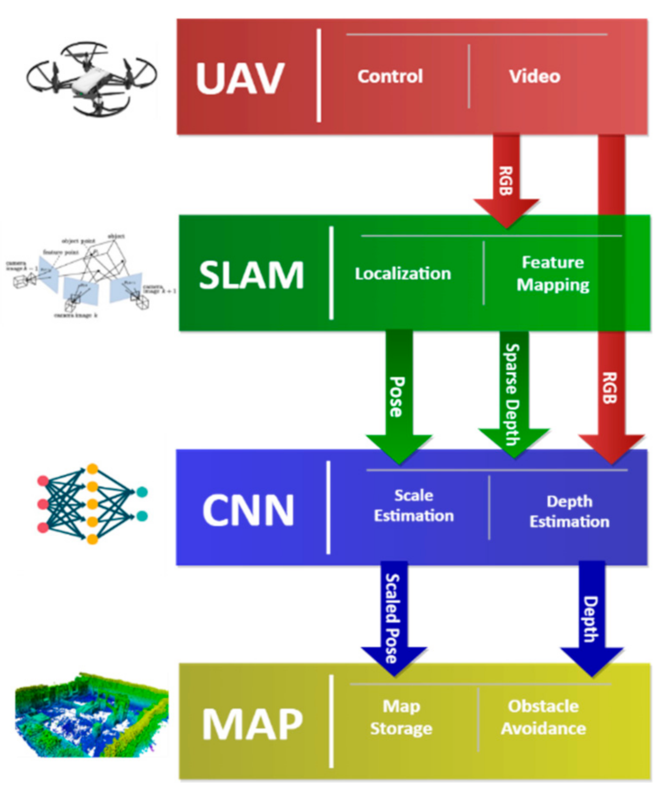
3. Methodology
3.1. Drone and Data Streaming
3.2. SLAM Algorithm
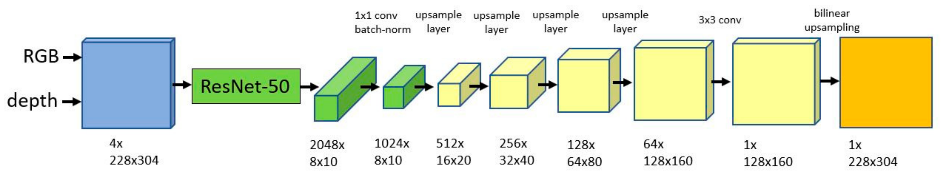
3.3. CNN-Based Densification and Scaling
3.3.1. CNN Training
3.3.2. Scale Initialization
3.4. Exploration Map
4. Tests and Results
4.1. Network Training
4.1.1. Sampling Density
4.1.2. Scale Estimation
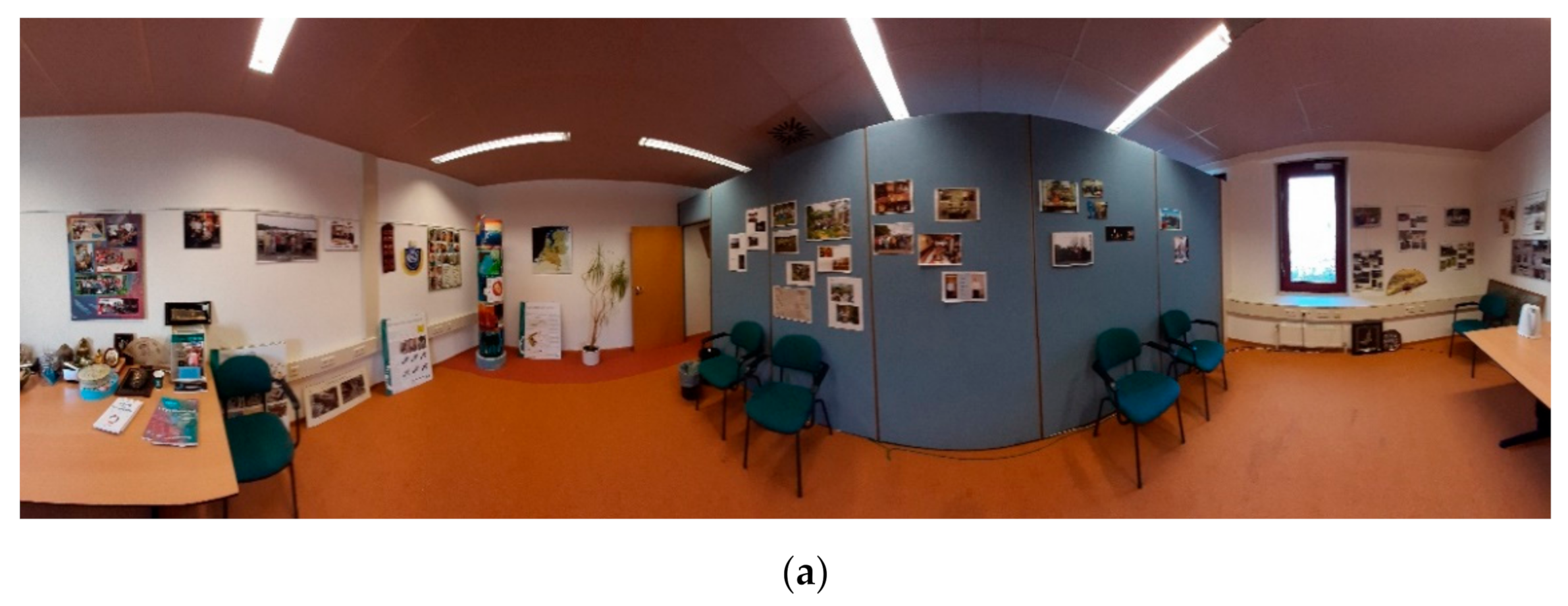
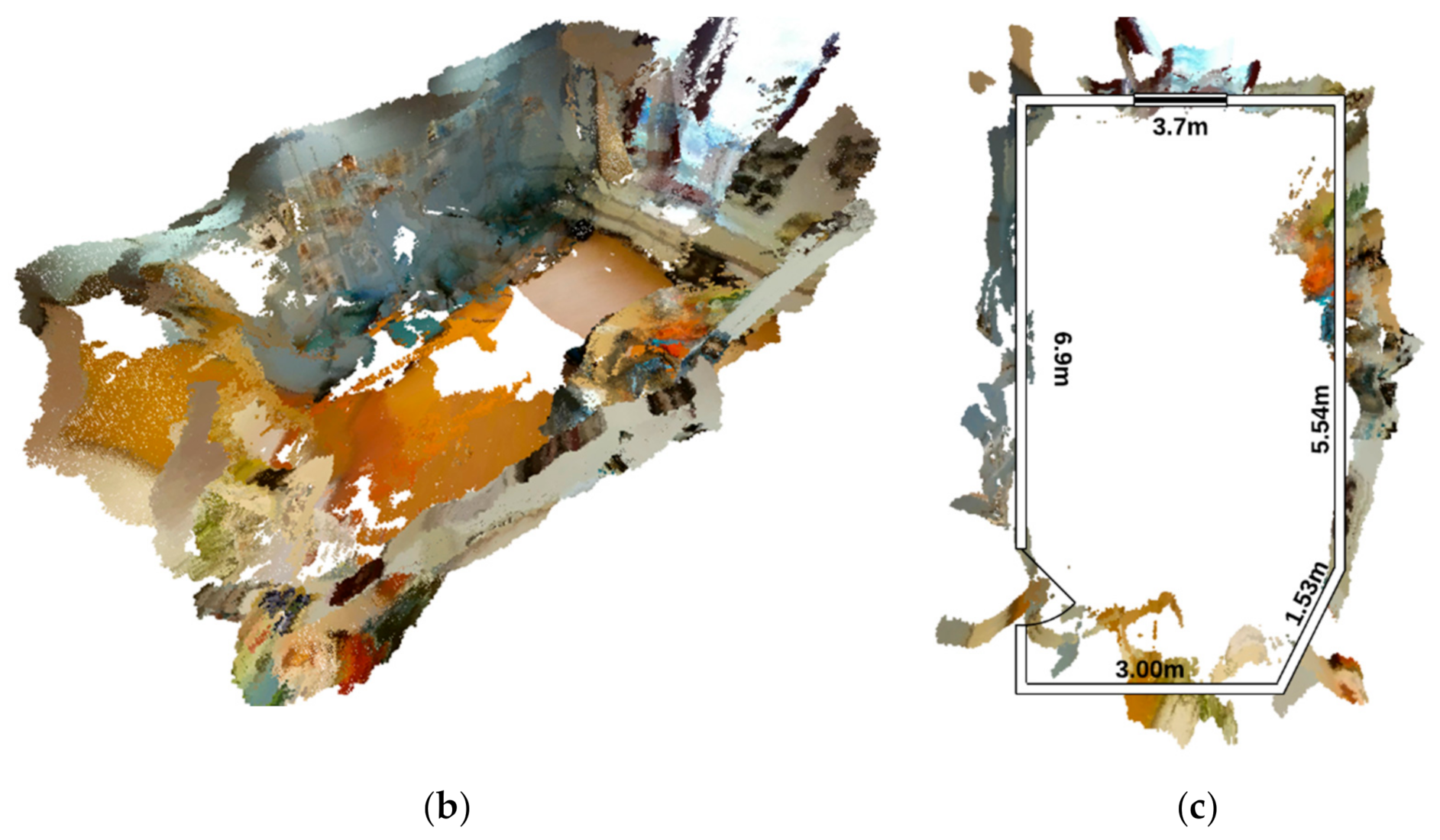
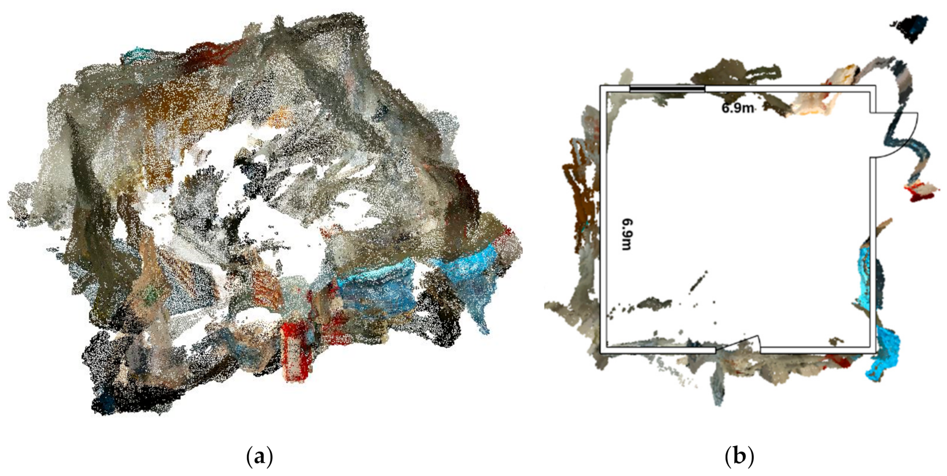
4.2. 3D Reconstruction of Test Environments—First Results
4.2.1. First Test
4.2.2. Second Test
5. Discussion
6. Conclusions and Future Developments
Supplementary Materials
Author Contributions
Funding
Conflicts of Interest
References
- Nex, F.; Duarte, D.; Steenbeek, A.; Kerle, N. Towards Real-Time Building Damage Mapping with Low-Cost UAV Solutions. Remote Sens. 2019, 11, 287. [Google Scholar] [CrossRef] [Green Version]
- Li, F.; Zlatanova, S.; Koopman, M.; Bai, X.; Diakité, A. Universal Path Planning for an Indoor Drone. Autom. Constr. 2018, 95, 275–283. [Google Scholar] [CrossRef]
- Sandino, J.; Vanegas, F.; Maire, F.; Caccetta, P.; Sanderson, C.; Gonzalez, F. UAV Framework for Autonomous Onboard Navigation and People/Object Detection in Cluttered Indoor Environments. Remote Sens. 2020, 12, 3386. [Google Scholar] [CrossRef]
- Khosiawan, Y.; Park, Y.; Moon, I.; Nilakantan, J.M.; Nielsen, I. Task Scheduling System for UAV Operations in Indoor Environment. Neural Comput. Appl. 2018, 31, 5431–5459. [Google Scholar] [CrossRef] [Green Version]
- Nex, F.; Armenakis, C.; Cramer, M.; Cucci, D.A.; Gerke, M.; Honkavaara, E.; Kukko, A.; Persello, C.; Skaloud, J. UAV in the Advent of the Twenties: Where We Stand and What Is Next. ISPRS J. Photogramm. Remote Sens. 2022, 184, 215–242. [Google Scholar] [CrossRef]
- Zhang, N.; Nex, F.; Kerle, N.; Vosselman, G. LISU: Low-Light Indoor Scene Understanding with Joint Learning of Reflectance Restoration. ISPRS J. Photogramm. Remote Sens. 2022, 183, 470–481. [Google Scholar] [CrossRef]
- Xin, C.; Wu, G.; Zhang, C.; Chen, K.; Wang, J.; Wang, X. Research on Indoor Navigation System of UAV Based on LIDAR. In Proceedings of the 2020 12th International Conference on Measuring Technology and Mechatronics Automation (ICMTMA), Phuket, Thailand, 28–29 February 2020; pp. 763–766. [Google Scholar]
- Lin, Y.; Hyyppä, J.; Jaakkola, A. Mini-UAV-Borne LIDAR for Fine-Scale Mapping. IEEE Geosci. Remote Sens. Lett. 2011, 8, 426–430. [Google Scholar] [CrossRef]
- Pu, S.; Xie, L.; Ji, M.; Zhao, Y.; Liu, W.; Wang, L.; Zhao, Y.; Yang, F.; Qiu, D. Real-Time Powerline Corridor Inspection by Edge Computing of UAV Linar Data. ISPRS Int. Arch. Photogramm. Remote Sens. Spat. Inf. Sci. 2019, 42, 547–551. [Google Scholar] [CrossRef] [Green Version]
- De Croon, G.; De Wagter, C. Challenges of Autonomous Flight in Indoor Environments. In Proceedings of the 2018 IEEE/RSJ International Conference on Intelligent Robots and Systems (IROS), Madrid, Spain, 1–5 October 2018; pp. 1003–1009. [Google Scholar]
- Falanga, D.; Kleber, K.; Mintchev, S.; Floreano, D.; Scaramuzza, D. The Foldable Drone: A Morphing Quadrotor That Can Squeeze and Fly. IEEE Robot. Autom. Lett. 2019, 4, 209–216. [Google Scholar] [CrossRef] [Green Version]
- Amer, K.; Samy, M.; Shaker, M.; Elhelw, M. Deep Convolutional Neural Network Based Autonomous Drone Navigation. In Proceedings of the Thirteenth International Conference on Machine Vision, Rome, Italy, 2–6 November 2020; Osten, W., Zhou, J., Nikolaev, D.P., Eds.; SPIE: Rome, Italy, 2021; p. 46. [Google Scholar]
- Arnold, R.D.; Yamaguchi, H.; Tanaka, T. Search and Rescue with Autonomous Flying Robots through Behavior-Based Cooperative Intelligence. J. Int. Humanit. Action 2018, 3, 18. [Google Scholar] [CrossRef] [Green Version]
- Bai, S.; Chen, F.; Englot, B. Toward Autonomous Mapping and Exploration for Mobile Robots through Deep Supervised Learning. In Proceedings of the 2017 IEEE/RSJ International Conference on Intelligent Robots and Systems (IROS), Vancouver, BC, Canada, 24–28 September 2017; IEEE: Piscataway, NJ, USA, 2017; pp. 2379–2384. [Google Scholar]
- Chakravarty, P.; Kelchtermans, K.; Roussel, T.; Wellens, S.; Tuytelaars, T.; Van Eycken, L. CNN-Based Single Image Obstacle Avoidance on a Quadrotor. In Proceedings of the 2017 IEEE International Conference on Robotics and Automation (ICRA), Singapore, 29 May–3 June 2017; IEEE: Piscataway, NJ, USA, 2017; pp. 6369–6374. [Google Scholar]
- Madhuanand, L.; Nex, F.; Yang, M.Y. Self-Supervised Monocular Depth Estimation from Oblique UAV Videos. ISPRS J. Photogramm. Remote Sens. 2021, 176, 1–14. [Google Scholar] [CrossRef]
- Knobelreiter, P.; Reinbacher, C.; Shekhovtsov, A.; Pock, T. End-To-End Training of Hybrid CNN-CRF Models for Stereo. In Proceedings of the Proceedings of the IEEE Conference on Computer Vision and Pattern Recognition (CVPR), Honolulu, HI, USA, 21–26 July 2017. [Google Scholar]
- Yang, M.Y.; Kumaar, S.; Lyu, Y.; Nex, F. Real-Time Semantic Segmentation with Context Aggregation Network. ISPRS J. Photogramm. Remote Sens. 2021, 178, 124–134. [Google Scholar] [CrossRef]
- Singandhupe, A.; La, H.M. A Review of SLAM Techniques and Security in Autonomous Driving. In Proceedings of the 2019 Third IEEE International Conference on Robotic Computing (IRC), Naples, Italy, 25–27 February 2019; pp. 602–607. [Google Scholar]
- Saeedi, S.; Spink, T.; Gorgovan, C.; Webb, A.; Clarkson, J.; Tomusk, E.; Debrunner, T.; Kaszyk, K.; Gonzalez-De-Aledo, P.; Rodchenko, A.; et al. Navigating the Landscape for Real-Time Localization and Mapping for Robotics and Virtual and Augmented Reality. Proc. IEEE 2018, 106, 2020–2039. [Google Scholar] [CrossRef] [Green Version]
- Stachniss, C.; Leonard, J.J.; Thrun, S. Simultaneous Localization and Mapping. In Springer Handbook of Robotics; Springer: Berlin/Heidelberg, Germany, 2016; pp. 1153–1176. ISBN 978-3-319-32552-1. [Google Scholar]
- Campos, C.; Elvira, R.; Rodríguez, J.J.G.; Montiel, J.M.M.; Tardós, J.D. ORB-SLAM3: An Accurate Open-Source Library for Visual, Visual-Inertial and Multi-Map SLAM. IEEE Trans. Robot. 2020, 37, 1874–1890. [Google Scholar] [CrossRef]
- Yang, N.; von Stumberg, L.; Wang, R.; Cremers, D. D3VO: Deep Depth, Deep Pose and Deep Uncertainty for Monocular Visual Odometry. In Proceedings of the IEEE Conference on Computer Vision and Pattern Recognition (CVPR), Seattle, WA, USA, 13–19 June 2020. [Google Scholar]
- Mur-Artal, R.; Tardos, J.D. ORB-SLAM2: An Open-Source SLAM System for Monocular, Stereo, and RGB-D Cameras. IEEE Trans. Robot. 2017, 33, 1255–1262. [Google Scholar] [CrossRef] [Green Version]
- Mur-Artal, R.; Tardos, J. Probabilistic Semi-Dense Mapping from Highly Accurate Feature-Based Monocular SLAM. In Proceedings of the Robotics: Science and Systems XI, Rome, Italy, 13–17 July 2015. [Google Scholar]
- Engel, J.; Schöps, T.; Cremers, D. LSD-SLAM: Large-Scale Direct Monocular SLAM. In Proceedings of the 13th European Conference of Computer Vision, Zürich, Switzerland, 6–12 September 2014; pp. 834–849. [Google Scholar]
- Von Stumberg, L.; Cremers, D. DM-VIO: Delayed Marginalization Visual-Inertial Odometry. IEEE Robot. Autom. Lett. 2022, 7, 1408–1415. [Google Scholar] [CrossRef]
- Gaoussou, H.; Dewei, P. Evaluation of the Visual Odometry Methods for Semi-Dense Real-Time. Adv. Comput. Int. J. 2018, 9, 1–14. [Google Scholar] [CrossRef] [Green Version]
- Qin, T.; Li, P.; Shen, S. VINS-Mono: A Robust and Versatile Monocular Visual-Inertial State Estimator. IEEE Trans. Robot. 2018, 34, 1004–1020. [Google Scholar] [CrossRef] [Green Version]
- Zeng, A.; Song, S.; Niessner, M.; Fisher, M.; Xiao, J.; Funkhouser, T. 3DMatch: Learning Local Geometric Descriptors from RGB-D Reconstructions. In Proceedings of the 2017 IEEE Conference on Computer Vision and Pattern Recognition (CVPR), Honolulu, HI, USA, 21–26 July 2017; pp. 199–208. [Google Scholar]
- Zhang, Z.; Zhao, R.; Liu, E.; Yan, K.; Ma, Y. Scale Estimation and Correction of the Monocular Simultaneous Localization and Mapping (SLAM) Based on Fusion of 1D Laser Range Finder and Vision Data. Sensors 2018, 18, 1948. [Google Scholar] [CrossRef] [Green Version]
- Tateno, K.; Tombari, F.; Laina, I.; Navab, N. CNN-SLAM: Real-Time Dense Monocular SLAM with Learned Depth Prediction. In Proceedings of the 2017 IEEE Conference on Computer Vision and Pattern Recognition (CVPR), Honolulu, HI, USA, 21–26 July 2017; pp. 6565–6574. [Google Scholar]
- Saxena, A.; Chung, S.H.; Ng, A.Y. Learning Depth from Single Monocular Images. In Proceedings of the Advances in Neural Information Processing Systems; 2005; pp. 1161–1168. Available online: http://www.cs.cornell.edu/~asaxena/learningdepth/NIPS_LearningDepth.pdf (accessed on 30 January 2022).
- Ming, Y.; Meng, X.; Fan, C.; Yu, H. Deep Learning for Monocular Depth Estimation: A Review. Neurocomputing 2021, 438, 14–33. [Google Scholar] [CrossRef]
- Laina, I.; Rupprecht, C.; Belagiannis, V.; Tombari, F.; Navab, N. Deeper Depth Prediction with Fully Convolutional Residual Networks. In Proceedings of the 2016 Fourth International Conference on 3D Vision (3DV), Stanford, CA, USA, 25–28 October 2016; pp. 239–248. [Google Scholar]
- Godard, C.; Mac Aodha, O.; Brostow, G.J. Unsupervised Monocular Depth Estimation With Left-Right Consistency. In Proceedings of the Proceedings of the IEEE Conference on Computer Vision and Pattern Recognition (CVPR), Honolulu, HI, USA, 21–26 July 2017. [Google Scholar]
- Mayer, N.; Ilg, E.; Hausser, P.; Fischer, P.; Cremers, D.; Dosovitskiy, A.; Brox, T. A Large Dataset to Train Convolutional Networks for Disparity, Optical Flow, and Scene Flow Estimation. In Proceedings of the IEEE Conference on Computer Vision and Pattern Recognition (CVPR), Las Vegas, NV, USA, 27–30 June 2016. [Google Scholar]
- Muglikar, M.; Zhang, Z.; Scaramuzza, D. Voxel Map for Visual SLAM. In Proceedings of the 2020 IEEE International Conference on Robotics and Automation (ICRA), Virtual Conference, 31 May–31 August 2020; pp. 4181–4187. [Google Scholar]
- Hornung, A.; Wurm, K.M.; Bennewitz, M.; Stachniss, C.; Burgard, W. OctoMap: An Efficient Probabilistic 3D Mapping Framework Based on Octrees. Auton. Robot. 2013, 34, 189–206. [Google Scholar] [CrossRef] [Green Version]
- Rublee, E.; Rabaud, V.; Konolige, K.; Bradski, G. ORB: An Efficient Alternative to SIFT or SURF. In Proceedings of the 2011 International Conference on Computer Vision, Barcelona, Spain, 6–13 November 2011; pp. 2564–2571. [Google Scholar]
- Rosten, E.; Porter, R.; Drummond, T. Faster and Better: A Machine Learning Approach to Corner Detection. IEEE Trans. Pattern Anal. Mach. Intell. 2010, 32, 105–119. [Google Scholar] [CrossRef] [PubMed] [Green Version]
- Ma, F.; Karaman, S. Sparse-to-Dense: Depth Prediction from Sparse Depth Samples and a Single Image. In Proceedings of the 2018 IEEE International Conference on Robotics and Automation (ICRA), Brisbane, Australia, 21–26 May 2018; pp. 4796–4803. [Google Scholar]
- He, K.; Zhang, X.; Ren, S.; Sun, J. Deep Residual Learning for Image Recognition. In Proceedings of the 2016 IEEE Conference on Computer Vision and Pattern Recognition (CVPR), Las Vegas, NV, USA, 27–30 June 2016; pp. 770–778. [Google Scholar]
- Silberman, N.; Hoiem, D.; Kohli, P.; Fergus, R. Indoor Segmentation and Support Inference from RGBD Images. In Computer Vision—ECCV 2012; Fitzgibbon, A., Lazebnik, S., Perona, P., Sato, Y., Schmid, C., Eds.; Springer: Berlin/Heidelberg, Germany, 2012; Volume 7576, pp. 746–760. ISBN 978-3-642-33714-7. [Google Scholar]
- Khoshelham, K.; Elberink, S.O. Accuracy and Resolution of Kinect Depth Data for Indoor Mapping Applications. Sensors 2012, 12, 1437–1454. [Google Scholar] [CrossRef] [Green Version]
- He, L.; Wang, G.; Hu, Z. Learning Depth from Single Images with Deep Neural Network Embedding Focal Length. IEEE Trans. Image Process. 2018, 27, 4676–4689. [Google Scholar] [CrossRef] [PubMed] [Green Version]
- Wurm, K.M.; Hornung, A.; Bennewitz, M.; Stachniss, C.; Burgard, W. Octomap: A Probabilistic, Flexible, and Compact 3D Map Representation for Robotic Systems. In Proceedings of the Autonomous Robots. 2010. Available online: https://www.researchgate.net/publication/235008236_OctoMap_A_Probabilistic_Flexible_and_Compact_3D_Map_Representation_for_Robotic_Systems (accessed on 30 January 2022).
- Sturm, J.; Engelhard, N.; Endres, F.; Burgard, W.; Cremers, D. A Benchmark for the Evaluation of RGB-D SLAM Systems. In Proceedings of the 2012 IEEE/RSJ International Conference on Intelligent Robots and Systems, Vilamoura-Algrave, Portugal, 7–12 October 2012; pp. 573–580. [Google Scholar]


| Tello Edu | 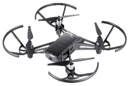 | |
| Camera | Photo: 5MP (2592 × 1936) Video: 720 p, 30 fps | |
| FOV | 82.6° | |
| Flight time | 13 min | |
| Remote control | 2.4 GHz 802.11 n WiFi | |
| Weight | 87 g |
| Points | MAE [m] | Abs rel | RMSE [m] | Time [s] | |
|---|---|---|---|---|---|
| 0 | 0.413 | 0.157 | 0.562 | 0.463 | 0.02 |
| 100 | 0.165 | 0.058 | 0.279 | 0.852 | 0.02 |
| 200 | 0.146 | 0.051 | 0.252 | 0.878 | 0.046 |
| 300 | 0.137 | 0.047 | 0.232 | 0.899 | 0.045 |
| 400 | 0.119 | 0.042 | 0.212 | 0.907 | 0.039 |
| Dataset | Ground Truth | CNN | Median Filter |
|---|---|---|---|
| TUM1 | 2.43 | 2.31 | 2.47 |
| TUM2 | 2.16 | 1.53 | 2.09 |
| TUM3 | 1.29 | 1.35 | 1.31 |
Publisher’s Note: MDPI stays neutral with regard to jurisdictional claims in published maps and institutional affiliations. |
© 2022 by the authors. Licensee MDPI, Basel, Switzerland. This article is an open access article distributed under the terms and conditions of the Creative Commons Attribution (CC BY) license (https://creativecommons.org/licenses/by/4.0/).
Share and Cite
Steenbeek, A.; Nex, F. CNN-Based Dense Monocular Visual SLAM for Real-Time UAV Exploration in Emergency Conditions. Drones 2022, 6, 79. https://doi.org/10.3390/drones6030079
Steenbeek A, Nex F. CNN-Based Dense Monocular Visual SLAM for Real-Time UAV Exploration in Emergency Conditions. Drones. 2022; 6(3):79. https://doi.org/10.3390/drones6030079
Chicago/Turabian StyleSteenbeek, Anne, and Francesco Nex. 2022. "CNN-Based Dense Monocular Visual SLAM for Real-Time UAV Exploration in Emergency Conditions" Drones 6, no. 3: 79. https://doi.org/10.3390/drones6030079
APA StyleSteenbeek, A., & Nex, F. (2022). CNN-Based Dense Monocular Visual SLAM for Real-Time UAV Exploration in Emergency Conditions. Drones, 6(3), 79. https://doi.org/10.3390/drones6030079