1. Introduction
For environmental sensing used for autonomous locomotion robots, sensors that can obtain metric information are used not merely for laser range finders (LRFs) and stereo cameras, but also for depth and visual sensors, such as red, green, blue, and depth (RGB-D) cameras [
1]. To estimate a self-position and to create an environmental map together from sensing signals with metric information, simultaneous localization and mapping (SLAM) [
2] has been studied widely as an effective and useful approach for indoor environments without using a global positioning system (GPS) for localization. Actually, SLAM is used practically and widely for cleaning robots, pet robots, and guide robots, but ground locomotion robots in terms of unmanned ground vehicles (UGVs) using wheels or crawlers have the effect of block-sensing from static or dynamic objects of various types in our environments of everyday life. Therefore, the accuracy of the vertical-axis map tends to be lower than that of the horizontal axis.
Recently, unmanned aerial vehicles (UAVs), which can fly freely in three-dimensional (3D) environments, have become increasingly popular-not merely for use as a hobby, but also for industrial applications [
3]. Assuming its main use for indoor flight with less wind influence, small airframe UAVs have been designated as micro air vehicles (MAVs). Compared with UGVs, MAVs have excellent sensing capability for the vertical axis because of their advanced locomotion capability and freedom. Nevertheless, because of the limited payload, it is a challenging task for MAVs to equip LRFs or stereo cameras, which can directly obtain metric information. Therefore, an approach to construct a 3D map using a monocular camera with structure from motion (SfM) [
4] has been attracting attention, especially in combination with MAVs [
5].
For the use of SfM, map construction accuracy depends strongly on the similarity of camera movements, visual fields, and scene features [
6]. Particularly, camera parameters and movements have the greatest effect among them. For example, a MAV obtains no metric information if flight patterns are less diverse. Moreover, 3D map creation using SfM is based on signal information that is similar to map creation using SLAM for position estimation [
7]. Semantic scene recognition is set to another task for robot vision studies [
8]. Improving autonomous flight accuracy for MAVs can be accomplished using a combination of 3D map creation with SfM and semantic scene recognition from appearance patterns on images with visual salience objects as visual landmarks [
9]. Semantic scene recognition has been studied widely as a subject-not merely for the advancement of computer vision studies [
10], but also for active robot vision studies, including MAV-based mobile vision studies.
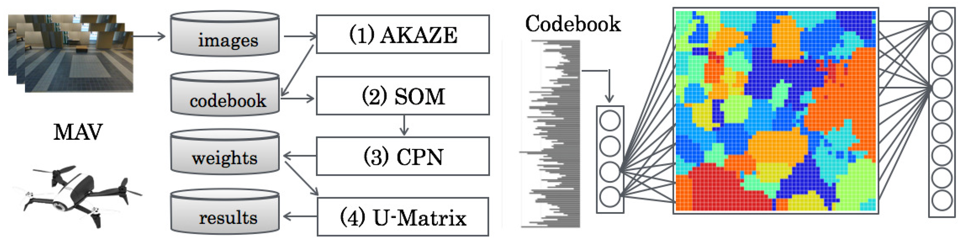
As an approach based on appearance changes using machine learning algorithms, this paper presents a vision-based indoor scene recognition method, as depicted in
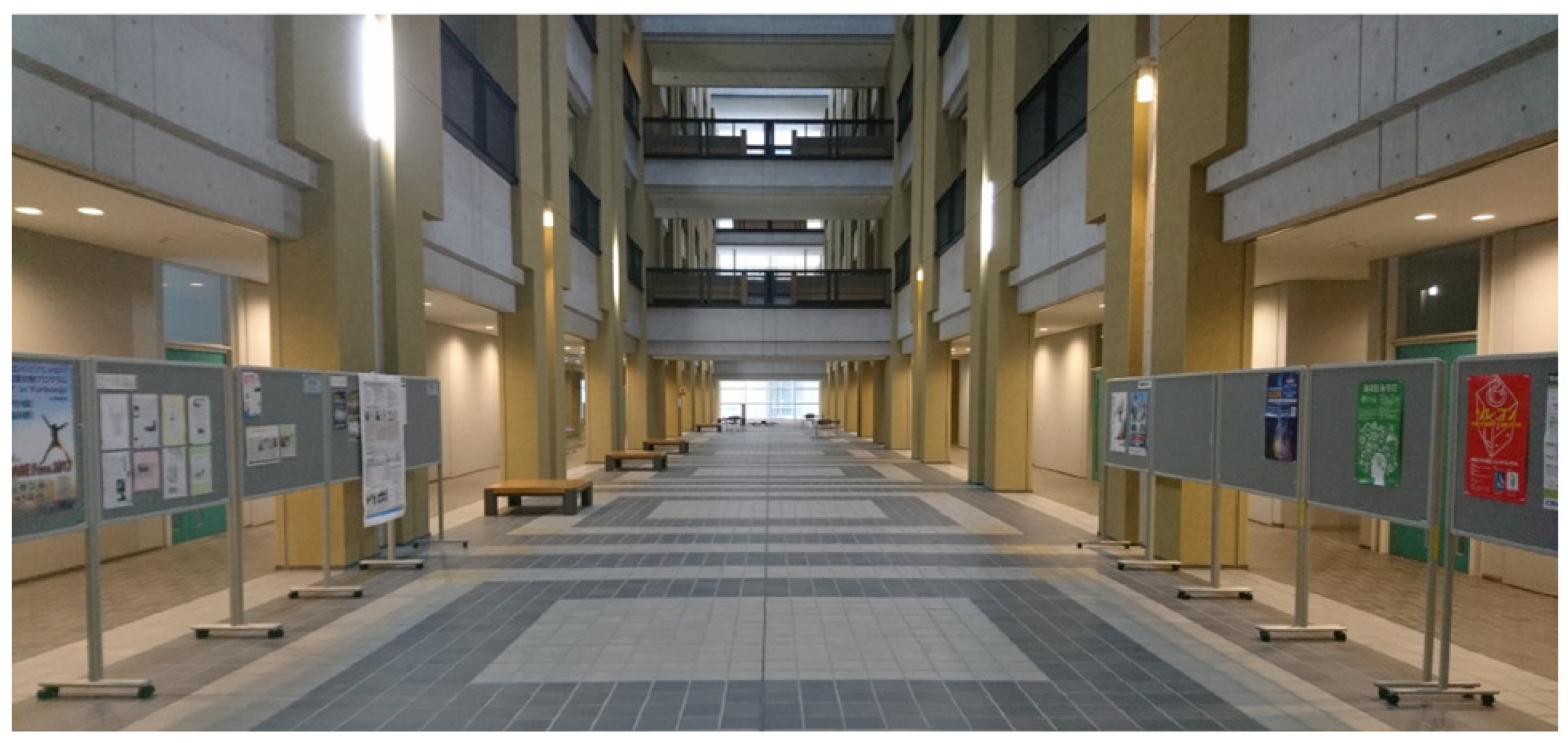
Figure 1 for aerial time-series images with a feature of visualization using a category map based on supervised learning. We used original benchmark datasets obtained in an atrium at our university building. The benchmark datasets comprise 10 zones as ground truth (GT) on two flight routes: a round flight route and a zigzag flight route. We evaluated the effectiveness of our method to demonstrate the recognition results of similarity and relation in each zone for visualization as category maps and their boundaries.
The rest of the paper is structured as follows. In
Section 2, related studies are presented, especially for monocular vision systems.
Section 3 and
Section 4 present our proposed method based on machine learning and our original indoor datasets obtained using a MAV, respectively. Subsequently,
Section 5 presents experimentally obtained results, including parameter optimization, confusion matrix analyses, and our discussion. Finally,
Section 6 presents our conclusions and highlights our future work. Herein, we proposed this basic method in the proceedings [
11]. For this paper, we present detailed results and a discussion in
Section 5.
2. Related Studies
In computer vision studies, numerous methods to recognize semantic scene categories from large numbers of static or dynamic images have been proposed [
12]. In general, their recognition targets were mainly in outdoor environments. Quattoni et al. [
13] reported that recognition accuracy drops dramatically if outdoor scene recognition methods are applied to indoor scene recognition. Assuming applications for human symbiotic robots, they play actively not merely in outdoor environments, but also in indoor environments. Improving recognition accuracy is necessary for semantic scene recognition methods that are applicable in indoor environments, especially for MAVs. Moreover, the environment for MAV locomotion as aerial robots changes in real time according to human activities and the diverse lifestyles of various people. Therefore, it must be used for MAVs not merely for environmental recognition and understanding, but also for adaptation capability according to environmental changes.
Numerous generalized methods using machine-learning algorithms have been proposed [
14] for environmental adaptation. Herein, machine learning is classified roughly into two types: supervised learning and unsupervised learning. Supervised learning requires training datasets annotated in advance with teaching signals such as GT. The burden related to teaching accompanies applying robots due to the obtaining of numerous training datasets in real time according to the tasks and actions. Moreover, the number of target recognition scene categories is set from teaching signals prepared in advance. In contrast, unsupervised learning classifies input datasets without teaching signals. After learning, semantic information is assigned from a part of datasets with GT for the use of a recognizer. For supervised learning methods, categories are extracted from various datasets obtained from environments. Compared with supervised learning methods, which require teaching signals in advance, the burden for teaching is reduced substantially, irrespective of the excessive number of learning data. Moreover, the number of categories was extracted automatically from training datasets according to the environments. Therefore, unsupervised learning has benefits for robotics applications, especially for robots collaborating with humans [
15].
As explained herein, unsupervised learning can construct knowledge frameworks autonomously as an intelligent robot [
16]. In actuality, neurons that selectively respond to human faces or cat faces were generated using deep learning (DL) frameworks [
17], which are attracting attention as a representative of unsupervised learning [
18]. We consider that unsupervised learning is useful for actualizing advanced communication and interaction between robots and humans.
The primary process for semantic scene recognition is to extract suitable scene features from image pixels in terms of brightness, color distribution, gradient, edge, energy, and entropy. As a global scene descriptor, Oliva et al. [
19] proposed Gist, which has been used widely for perspective scene feature description. However, the recognition accuracy drops dramatically in indoor environments that include numerous small objects because Gist is used for describing comprehensive structures in terms of roads, mountains, and buildings in outdoor environments [
13]. As an alternative approach, foreground and background features are used for context-based scene-recognition methods. Quattoni et al. [
13] proposed a method to describe features of a spatial pyramid using scale-invalid feature transform (SIFT) [
20] as foreground features and Gist [
19] as background features. They evaluated their method using a benchmark dataset for 67 indoor categories. Although the maximum recognition accuracy in the scene category of inside a church was 63.2%, the recognition accuracies in the scene categories of a jewelry shop, laboratory, mall, and office were 0%.
Madokoro et al. [
21] proposed a context-based scene recognition method using two-dimensional (2D) histograms as visual words (VWs) [
22] for voting Gist and SIFT on a 2D matrix. They demonstrated the effectiveness on indoor semantic scene recognition and the superiority of recognition accuracy compared with existing methods evaluated using the KTH-IDOL2 benchmark dataset [
23]. Moreover, they proposed a robust semantic scene recognition method for human effects using histogram of oriented gradient (HOG) [
24] features [
25]. However, both studies included evaluation experiments using a unmanned aerial vehicle (UGV)- based mobile robot. Although they evaluated occlusion and corruption among objects from the perspective of object recognition using an MAV [
26], they presented no result obtained from applying their MAV-based platform and machine-learning-based methods for scene recognition. Anbarasu et al. [
27] proposed a recognition method using support vector machines (SVMs) [
28] after describing scene features using Gist and histogram of directional morphological gradients (HODMGs) for aerial images obtained using a MAV. They conducted evaluation experiments using their originally collected datasets. Although they obtained sufficient recognition accuracies, recognition targets were merely three scene categories: corridors, staircases, and rooms.
3. Proposed Method
Our proposed method based on part-based features and supervised learning, as depicted in
Figure 1, comprises four steps:
- (1)
Feature extraction using AKAZE;
- (2)
Codebook generation using SOMs;
- (3)
Category map generation using CPNs;
- (4)
Category boundary extraction using U-Matrix.
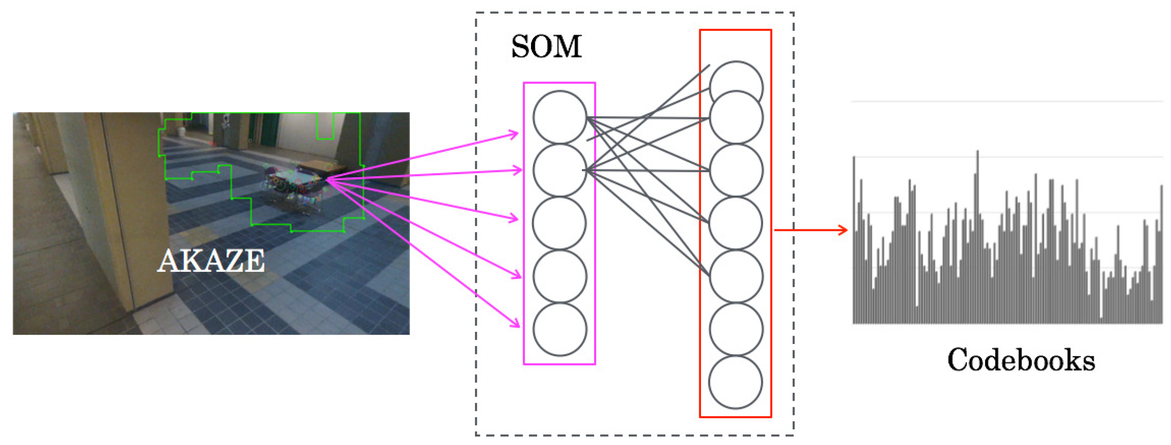
First, part-based features were extracted from aerial time-series scene images using accelerated KAZE (AKAZE) descriptors [
29]. Subsequently, VWs based on bags of keypoints [
30] were generated using self-organizing maps (SOMs) [
31] as codebooks with the integrated feature dimension, as depicted in
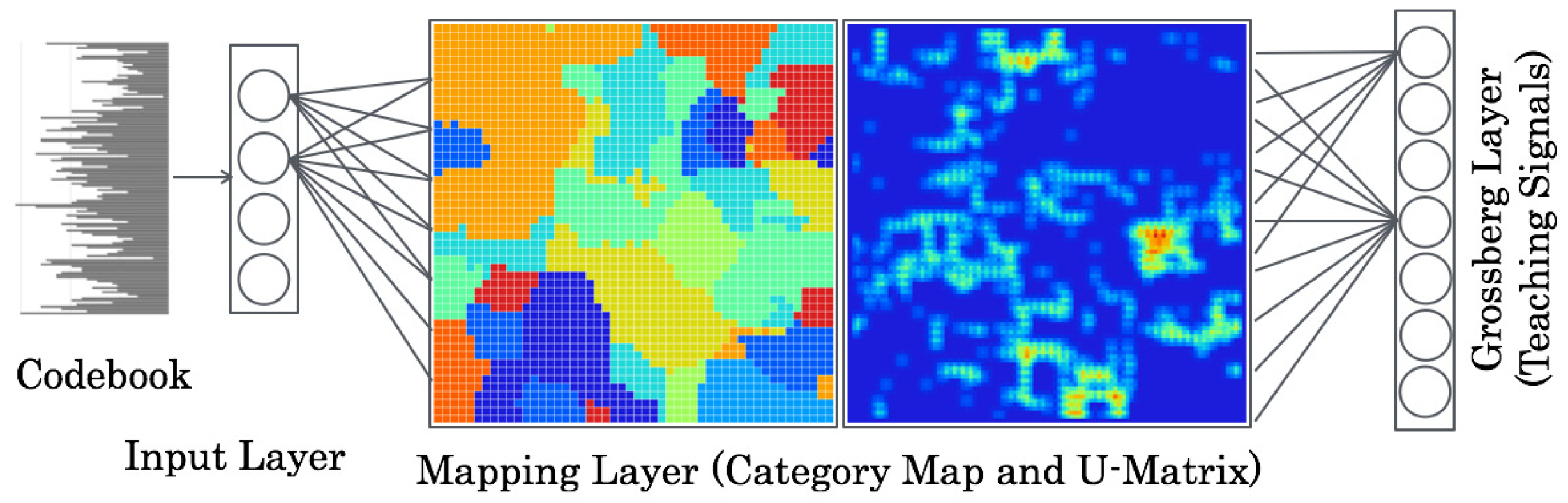
Figure 2. For creating category maps, VWs were presented to counter propagation networks (CPNs) [
32] as input features. For our method, scene relational features were visualized on category maps [
33] because of topological mapping of spatial scene relations, as depicted in
Figure 3. Finally, category boundaries were extracted using a unified distance matrix (U-Matrix) [
34] from weights between the input layer and the mapping layer on CPNs for extracting categories according to scene features.
Our method extracts scene categories for visualizing boundary depth after calculating the similarity of neighborhood categories mapped as category maps on CPNs. Detailed procedures of our method, which consists of three machine-learning algorithms with supervised and unsupervised modes, were presented in an earlier report [
33] For this paper, we used the network as the supervised mode.
3.1. SOMs
As depicted in
Figure 2, the network architecture of SOMs comprises two layers: an input layer and a mapping layer. Input signals are presented to the input layer. No teaching signals are presented to the mapping layer because of unsupervised learning.
The learning algorithm of SOMs is the following.
and
respectively denote input data and weights from an input layer unit
i to a mapping layer unit
j at time
t. Herein,
I,
J respectively denote the total numbers of the input layer and the mapping layer.
were initialized randomly before learning. The unit for which the Euclidean distance between
and
is the smallest is sought as the winner unit of its index
c as:
As a local region for updating weights, the neighborhood region
is defined as the center of the winner unit
c, as:
Therein, is the initial size of ; O is the maximum iteration for training. Coefficient 0.5 is appended as the floor function for rounding.
Subsequently,
of
was updated to close input feature patterns.
Therein,
is a learning coefficient that decreases along with the progress of learning.
is the initial value of
.
is defined at time
t as:
In the initial stage, the learning speed is higher when this rate is high. In the final stage, the learning converges while the range decreases.
For this module, the input features of
I dimension are quantized into the
J dimension, which is a similar dimension to the number of units on the mapping layer. The module output
is calculated as:
This module is connected to the labeling module at the training phase. For the testing phase, this module is switched to the mapping module. Moreover, this module is passed when input features are used without creating codebooks directly.
3.2. CPNs
As depicted in
Figure 3, the network architecture of CPNs comprises three layers: an input layer, a mapping layer, and a Grossberg layer. The input layer and mapping layer resemble those of SOMs. Teaching signals are presented to the Grossberg layer.
The learning algorithm of CPNs is the following. Herein, for visualization characteristics of category maps, we set the mapping layer to a two-dimensional structure
unit. For this paper, we set one dimension of the input and Grossberg layers, although they can take any structure. The numbers of units are
I and
K, respectively.
are weights from an input layer unit
i to a mapping layer unit
at time
t.
are weights from a Grossberg layer unit
k to a mapping layer unit
at time
t. These weights are initialized randomly before learning.
are training data to present to the input layer unit
i at time
t. The unit for which the Euclidean distance between
and
is the smallest is sought as the winner unit. c(x,y) is the index of the unit.
The neighborhood region
around
is defined as:
where
is the initial size of the neighborhood region, and
O is the maximum iteration for training.
of
were updated to close input feature patterns using Kohonen’s learning algorithm as:
Subsequently,
of
were updated to close teaching signal patterns using Grossberg’s learning algorithm.
Herein,
are training signals obtained using ART-2.
and
are learning coefficients that have decreasing values with the progress of learning.
and
denote the initial values of
and
, respectively. The learning coefficients are given as:
In the initial stage, the learning is done rapidly when the efficiencies are high. In the final stage, the learning converges, although the efficiencies decrease. As the maximum number of
for the
k-th Grossberg unit, category
is searched as:
A category map is created after determining categories for all units. Test datasets are presented to the network that is created through learning. A mapping layer unit, which is the minimum of the Euclidean distance as the similarity of test data and feature patterns, is burst. Categories for these units are recognition results for CPNs.
5. Evaluation Experiment
5.1. Parameter Optimization
As a preliminary experiment, we optimized three major parameters that influence the recognition accuracy. For evaluation criteria, recognition accuracy recognition accuracy
R [%] for a validation dataset is defined as:
where
C and
N respectively represent the total numbers of validation images and correct recognition images that matched to zone labels such as GT.
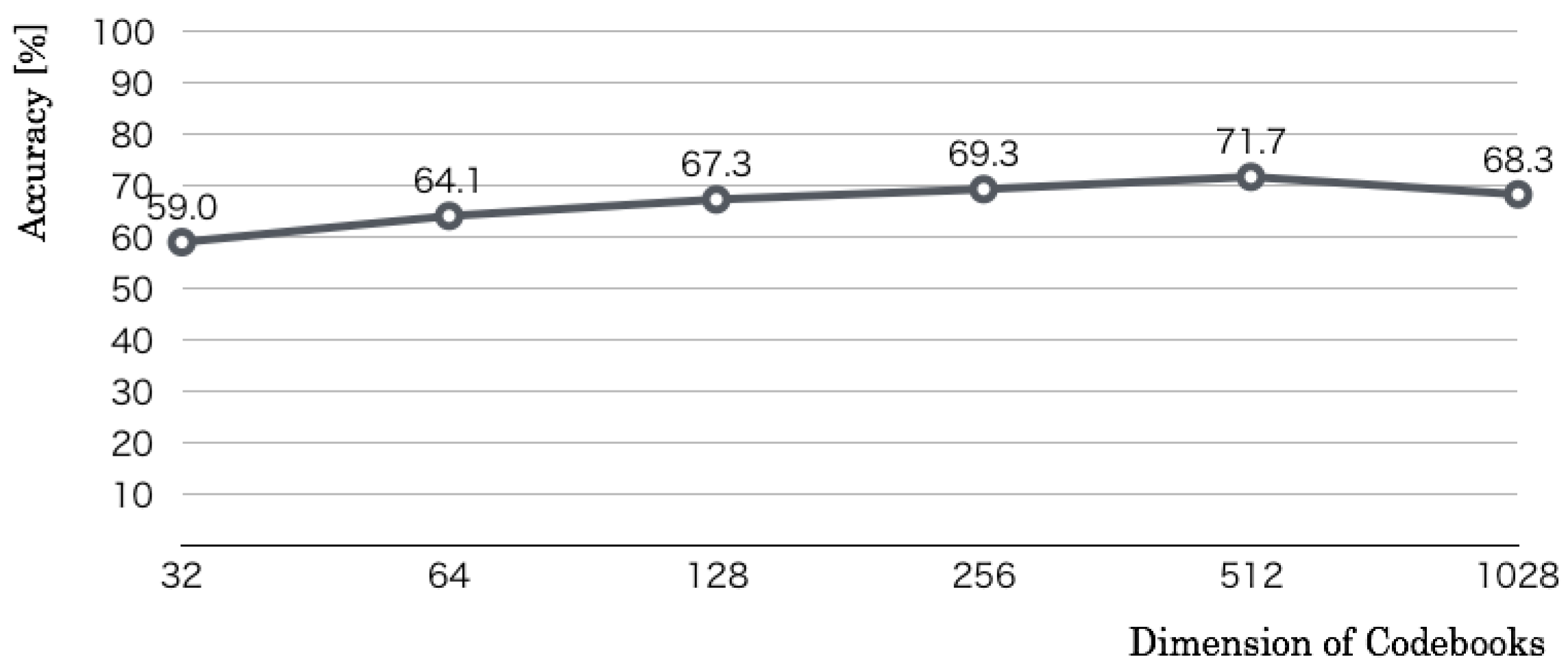
We used RFDs for this optimization. The first optimization parameter was codebook dimensions of input features. Whereas the size of a category map and the number of learning iterations were set, respectively, to 50 × 50 units and 10,000 iterations, we changed the coefficient
n of the codebook dimension
from Steps 5 to 10 by 1. The optimization result, as denoted in
Figure 10 revealed that the recognition accuracy increased according to increased
n. The maximum accuracy was 71.7% in
, which corresponds to 512 codebook dimensions.
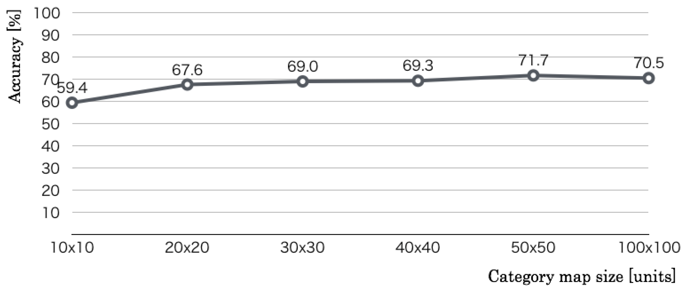
The second optimization parameter is the number of category map units. Whereas the codebook size and the number of learning iterations were set, respectively, to 256 dimensions and 10,000 iterations, we changed the category map units from 10 × 10 units to 60 × 60 units in 10 × 10 unit intervals. The optimization result, as denoted in
Figure 11 revealed that the recognition accuracy increased according to the category map size. The maximum accuracy was 71.7% in 50 × 50 category map units, which corresponds to the 512 codebook dimensions.
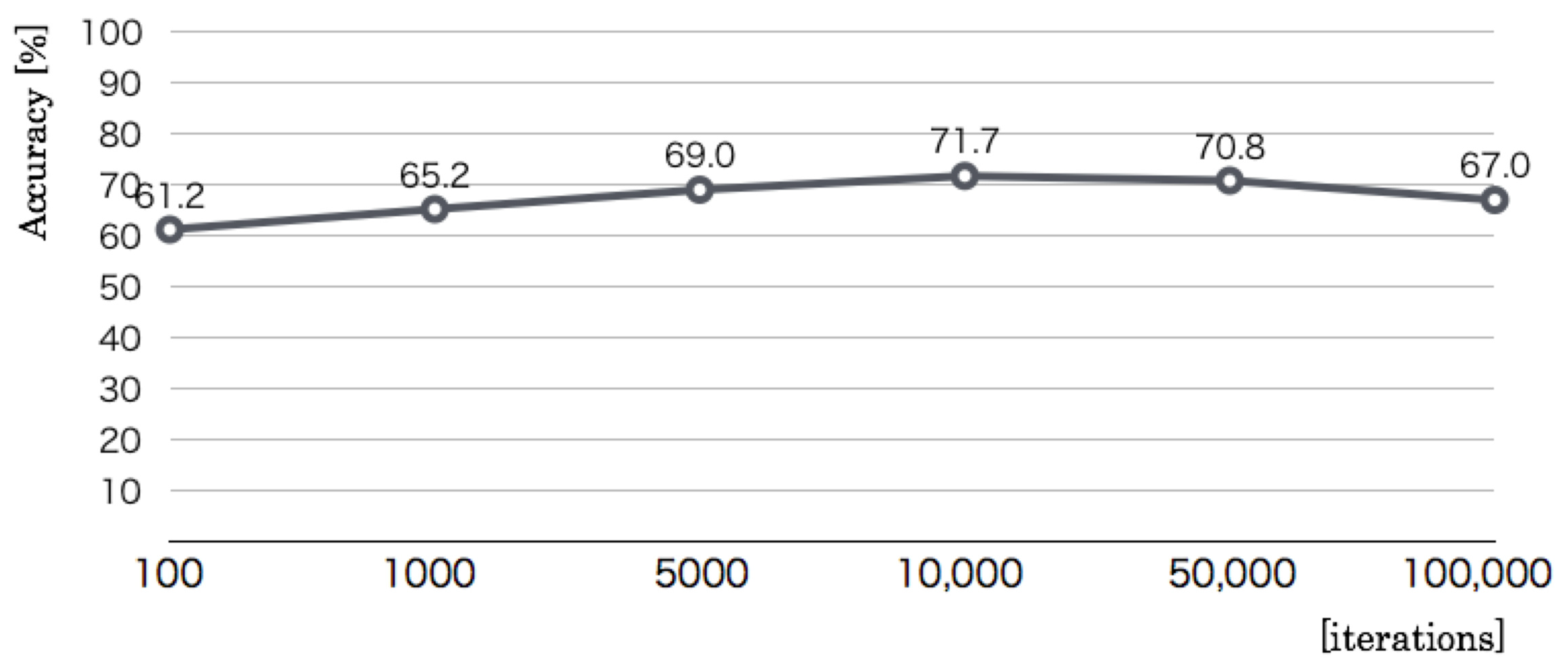
The third optimization parameter is the number of learning iterations. Whereas the codebook size and the size of a category map were set, respectively, to 256 dimensions and 50 × 50 units, we changed the learning iterations of five steps: 100, 1000, 5000, 10,000, 50,000, and 100,000. The optimization result, as denoted in
Figure 12 revealed that the recognition accuracy increased according to the iterations up to 10,000. The maximum accuracy was 71.7% in 10,000, which corresponds to the 512 codebook dimensions and 50 × 50 category map units. The results of the above three preliminary experiments showed that we used 512 codebook dimensions, 50 × 50 category map units, and 10,000 learning iterations as optimal values.
5.2. Created Category Maps
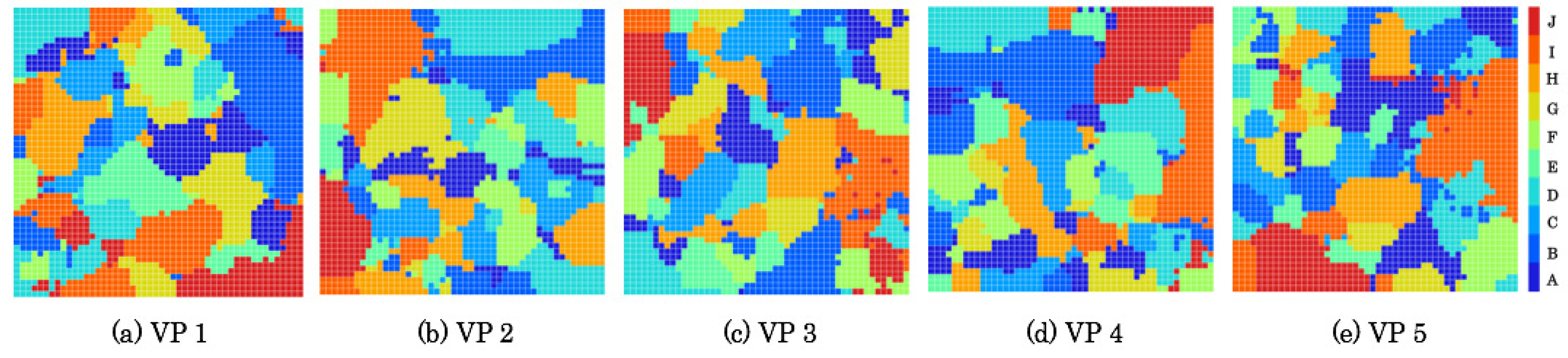
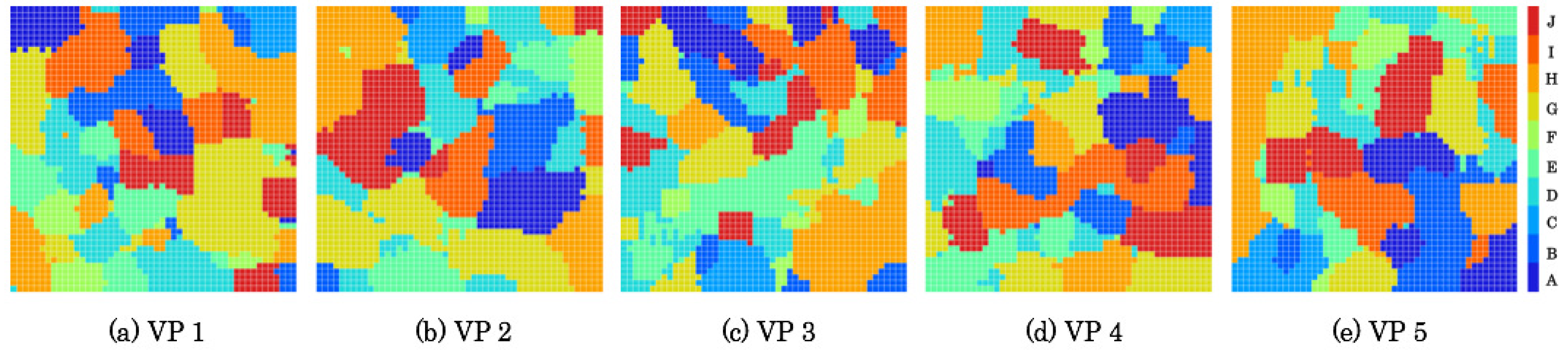
Figure 13 and
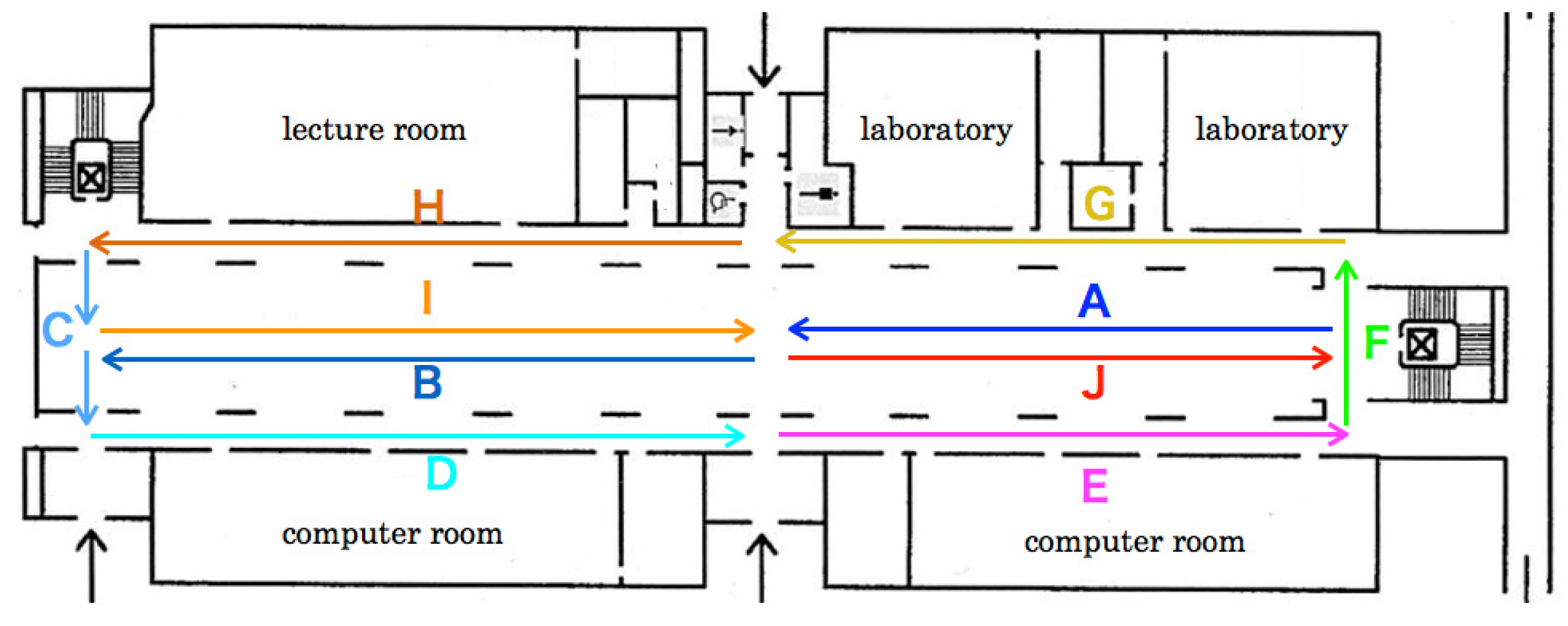
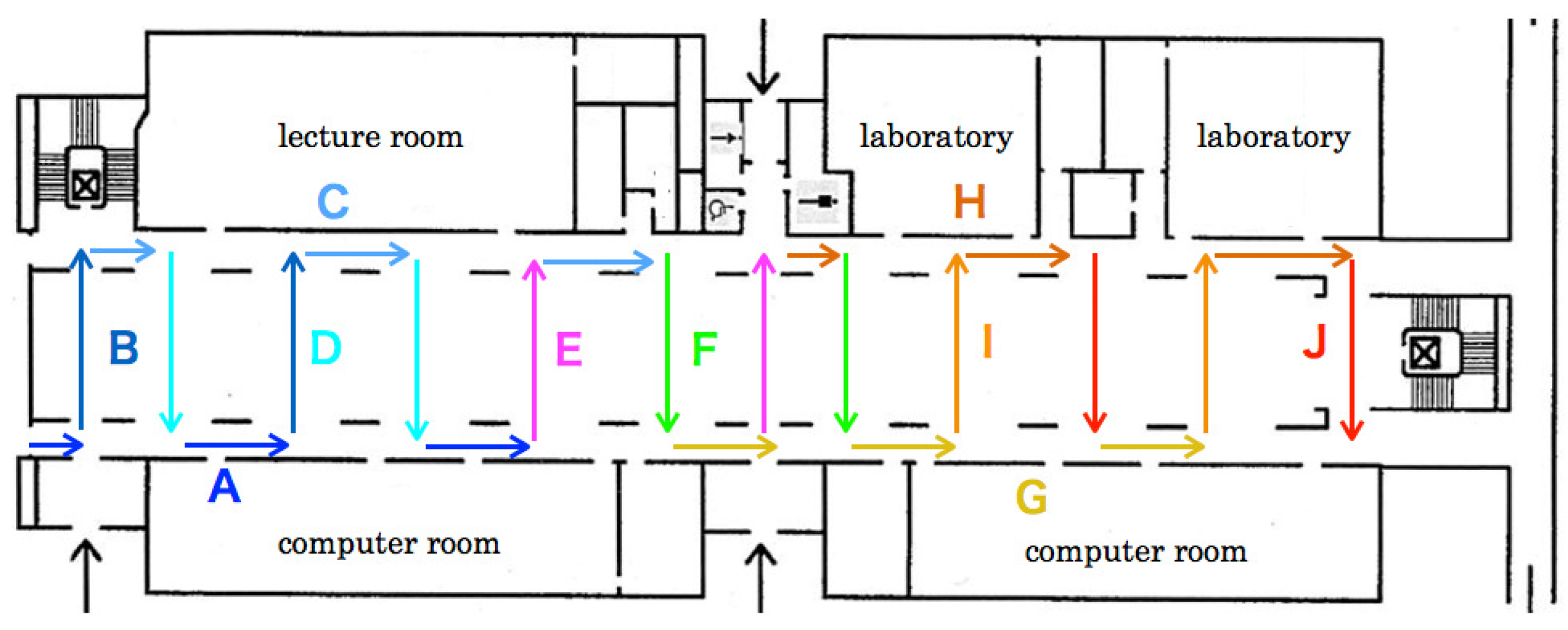
Figure 14 respectively depicts category maps created from RFDs and ZFDs. Categories are shown using heat maps according to color temperatures of ten steps. Zones A and J are allocated, respectively, to the lowest and the highest temperature colors. According to the progress of flight zones, as depicted in
Figure 6 and
Figure 7, categories corresponding with zones were changed from low-temperature colored units to high-temperature colored units in heat maps. After learning, category maps are used for recognizers.
Category maps were divided into several categories of respective zones with categorical representation reflected in scene complexity. The category maps of ZFDs denote higher scene complexity than those of RFDs because of segmented categories. Moreover, the category maps denote not merely high complexity of category boundaries, but also distributional characteristics to different positions with similar zones. Because category maps are created from training datasets, a single unit bursts from a test dataset based on the mechanism of winner-take-all (WTA) competition that obtains everything by a winner neuron. The label of a WTA unit is judged in terms of recognition results.
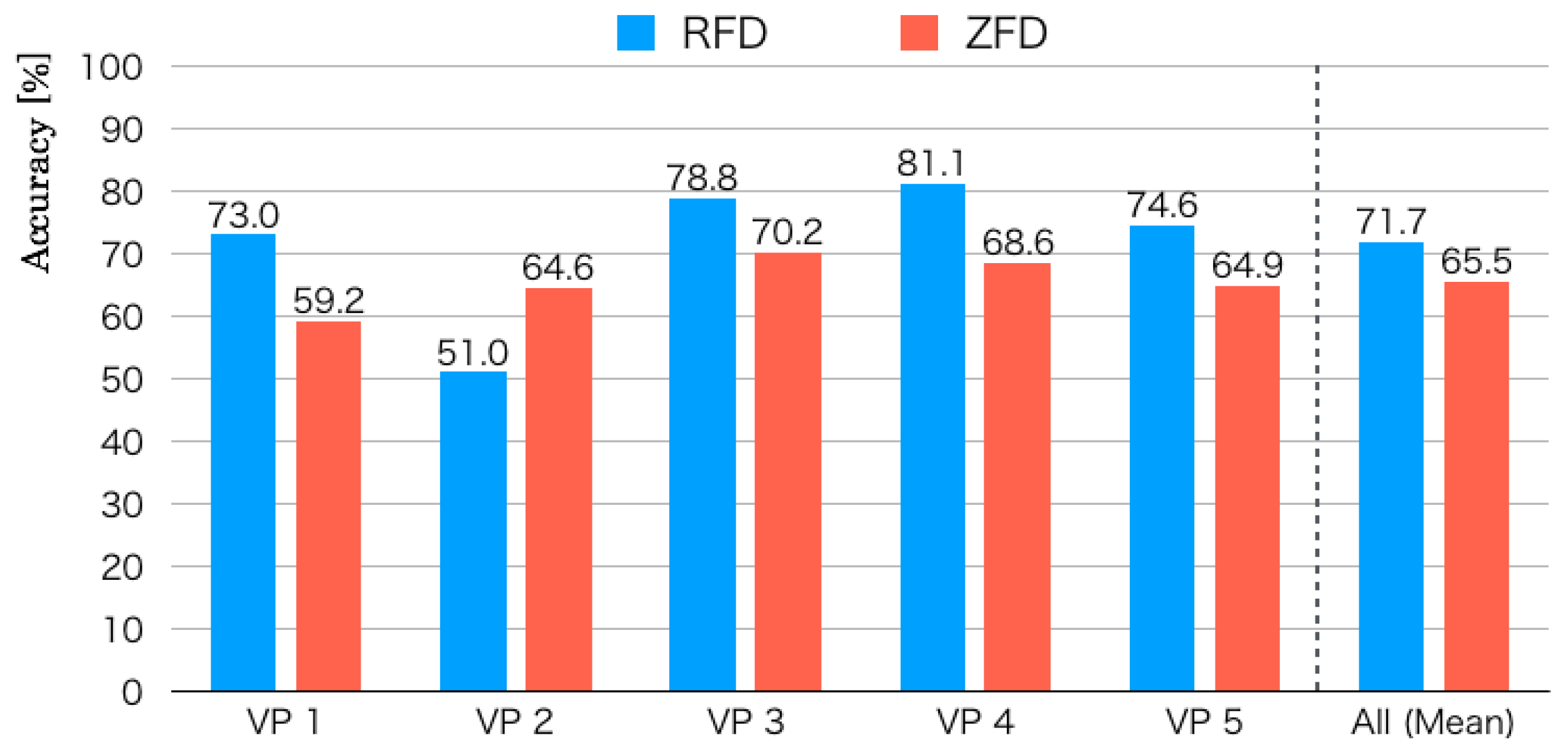
5.3. Recognition Results
Figure 15 depicts recognition accuracies for five LOOCV patterns. The mean recognition accuracy of RFDs was 71.7% for five datasets evaluated using LOOCV. The maximum and minimum recognition accuracies were, respectively, 81.1% for VP 4 and 51.0% for VP 2. The accuracy gap separating them was 27.8%. The recognition accuracy in Zone D of VP 4 is the lowest. Herein, we analyze false recognition tendencies from scene image features and flight routes. Numerous images in Zone D were falsely recognized to Zones E and I.
Figure 6 shows that the flight route from Zone D to Zone E comprised a passage between pillars and walls. Feature changes in these zones were slight compared with those in other zones. Moreover, numerous similar scene features existed because green doors for the computer rooms are lined up continuously. The flight orientation in Zone I was the same as that in Zone D, which included salient objects in the atrium to the scene images. We consider that false recognition occurred from objects in terms of chairs and tables that exist in Zone I as landmarks.
As the lowest recognition accuracy, images in Zones D, E, and G of VP 2 were falsely recognized as Zone J. Zones D, E, and G were a straight pathway between pillars and walls. False recognition images included a partial view to the center of the atrium that can be seen from pillars. In contrast, Zone J comprised a route, of which the MAV flew to the center of the atrium. For obtaining images of Dataset 2, the MAV flew to the pillar side compared with other datasets. Therefore, we infer that false recognition occurred from images between the pillars.
The mean recognition accuracy for five datasets of ZFDs was 65.5%, which was 6.2 percentage points lower than that of the RFDs. The scene complexity of the zigzag flight route was greater than that of the round flight route because it included numerous 90 degree rotations. The salient features in the ZFDs were fewer than in the RFDs because the MAV flew mainly in a lateral direction to both walls in the atrium. The maximum and minimum recognition accuracies were, respectively, 70.2% for VP 3 and 59.2% for VP 1. The gap separating them was 11.0%, which was lower than that of the RFDs.
False recognition was high for VP 3 in Zone H. As depicted in
Figure 7, the flight orientation is similar in Zones H and G with different routes. Objects on the scene images in both zones included pillars and doors merely because the flight route existed between pillars and walls. We infer that false recognition occurred from numerous similar scene features and their slight changes. Numerous images in Zone H were falsely recognized as Zone A or C. We infer that false recognition occurred from scene feature similarity.
For VP 1, with the lowest recognition accuracy, numerous images between Zones H and G and between Zones B and F were falsely recognized. However, falsely recognized images in Zone G were slight, except those of Zone H. We consider that salient features of pedestrians, desks, and sign boards are included in Zone H. In Zones B and F, the MAV flew a straight route to both walls of the lateral side in the atrium in opposite directions. The scene images in Zone F that were falsely recognized as Zone F included white walls, of which numerous features were overlapped in the different zones. In contrast, false recognition images in Zone B were slightly allocated to other zones except for Zone F.
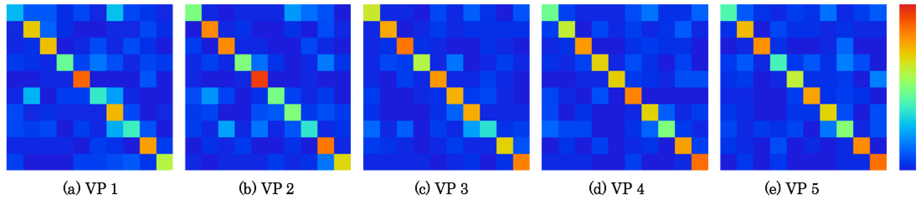
5.4. Confusion Matrix Analysis
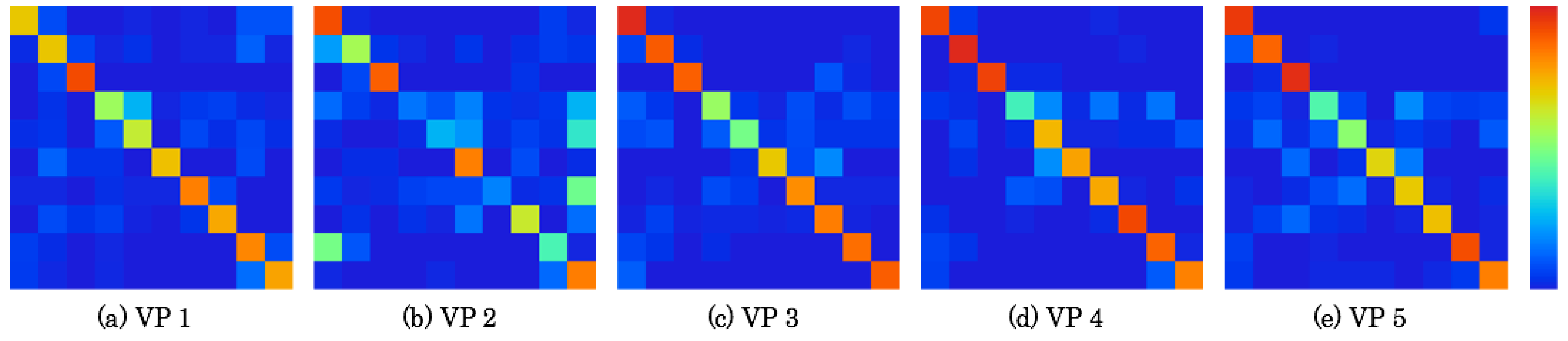
Figure 16 and
Figure 17 respectively depict confusion matrixes as detailed results of recognition accuracies, as presented in
Figure 15. The matrices comprise 10 rows × 10 columns that correspond to the number of segmented zones. The data existence rates on the matrixes are represented using heat maps. Correct numbers of images are represented on the diagonal matrix elements. The false recognition rate is high if the color temperature is high on the elements, except for the diagonal elements. For the base of the horizontal lines, false recognition images can be specified to the positions of vertical elements. A comprehensive tendency is that false recognition images are apparently numerous on the elements near the diagonal elements because scene features are changed sequentially according to the MAV flight.
Table 3 presents a confusion matrix of VP 4, which has the highest recognition accuracy in the RFD. The bold numbers represent the maximum number of images in each zone. For this result, the maximum number of images is distributed on the diagonal elements. Particularly, false recognition images in Zone D were more numerous than in other zones. In all, 52 of 86 images in Zone D were falsely recognized to other zones, including 16 false recognition images to Zone E. In contrast, other zones were recognized correctly, especially in Zones B and C, which were recognized correctly except for the numbers of images for one image in Zone B and three images in Zone C.
Table 4 denotes a confusion matrix of VP 2, which has the lowest recognition accuracy. The bold numbers, which demonstrate the maximum numbers of images, are available on the diagonal elements. The numbers of false recognition images in Zones D, E, and G were, respectively, 89 of 105 images, 61 of 82 images, and 67 of 81 images. Particularly, 27, 30, and 38 images in these zones were commonly falsely recognized as Zone J. However, false recognition images between Zones C and F were merely six.
We obtained a similar tendency from detailed confusion matrixes in the ZFD. Therefore, we consider that the arbitrary categories selected were not sufficiently distinct as to be separable in image space.
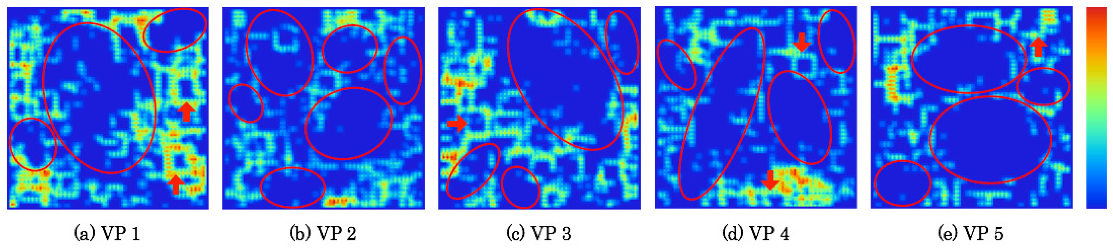
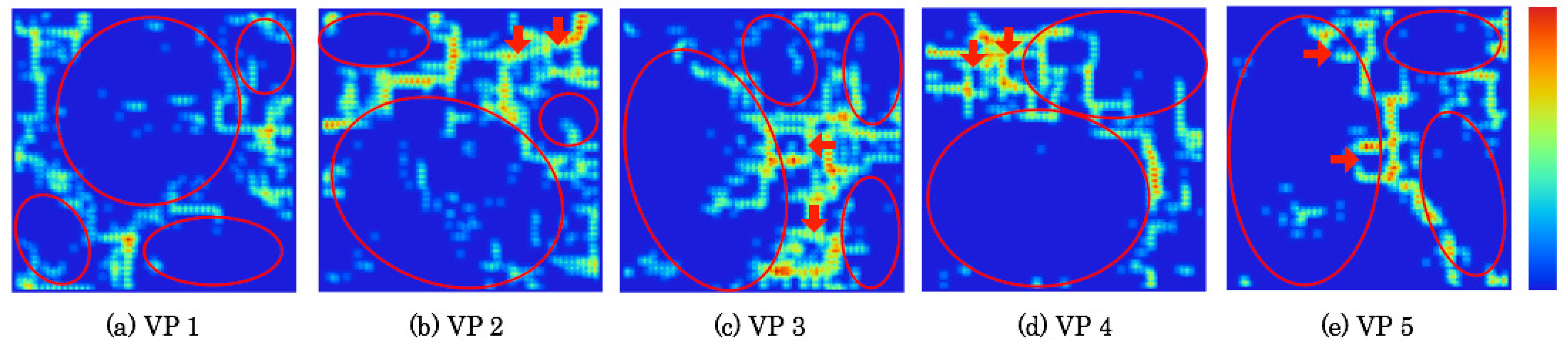
5.5. Extracted Category Boundaries
Based on weights between the input layer and the mapping layer on CPNs, category boundaries were extracted with a U-Matrix that calculates the similarity of neighborhood units.
Figure 18 and
Figure 19 respectively depict extraction results of category boundaries on category maps as depicted in
Figure 13 and
Figure 14. The depth of category boundaries is depicted using heat maps. Category boundaries of much weight difference among units are depicted in a high-temperature near-red color. Herein, slight output signals shown as low-temperature near-blue color were reduced automatically using a threshold extracted using the Otsu Method [
38].
The red ellipses on respective category maps denote comprehensive categories. The extraction results demonstrate that up to six categories were created with discontinuity boundaries and dependent units. The red-filled arrows denote local categories. As shown in category maps depicted in
Figure 13 and
Figure 14, the first and second neighborhood regions up to 25 units correspond to the respective local categories. In the next section, we attempt to discuss how many actual categories there are in the image space.
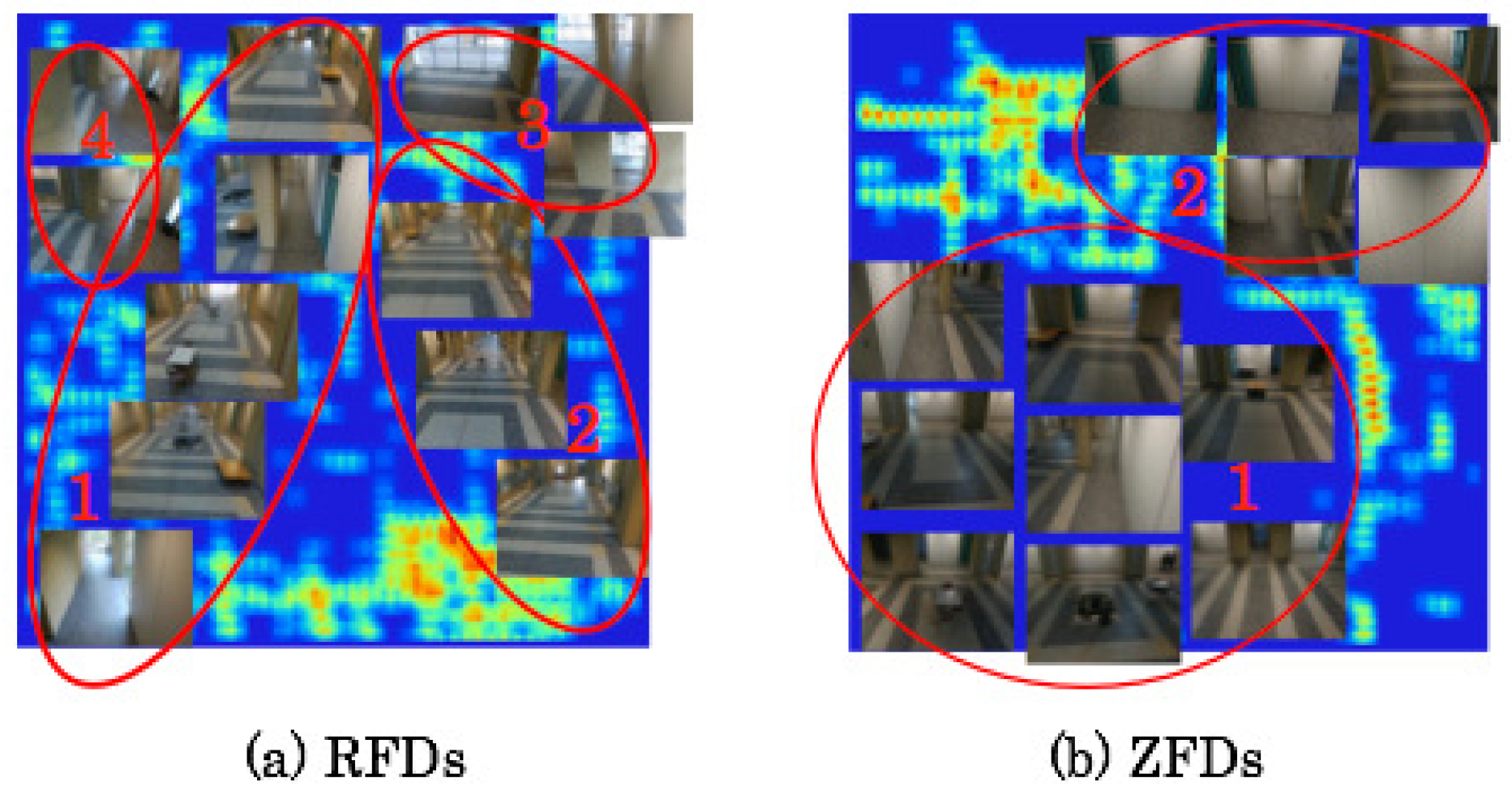
5.6. Discussion
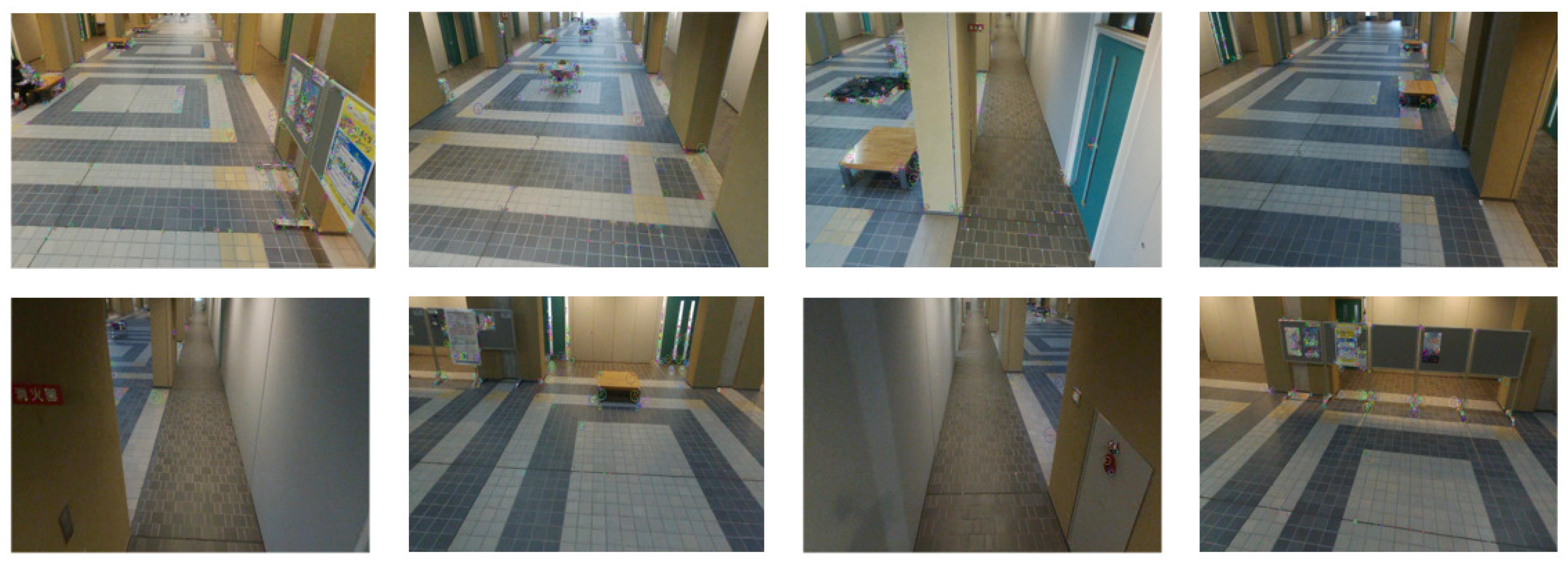
We attempted to analyze mapping characteristics of our method using superimposed scene images as a visual observation. As a mapping result, category boundaries were extracted using the U-Matrix. Up to eight typical scene images are shown on independent categories segmented by the category boundaries.
Figure 20a depicts representative images in each category superimposed on category boundaries obtained from VP 4 of RFDs. The category map was segmented to two comprehensive categories, as shown in
Figure 18d by red ellipses. We annotated numbers from the order of category sizes as Categories 1–4 in
Figure 20a. Scene images related to the longitudinal direction were mapped to Categories 1 and 2. Numerous scene images that include objects are present in Category 1. Moreover, several scene images in which the MAV flew the lateral direction of the center of the atrium in Zone F were in Category 1.
In contrast, Category 2 had numerous scene images without objects. Although Category 2 included images with objects, these were not merely small objects because of their distant location, but also a part of the background, which is difficult to distinguish. We inferred that this feature difference divided images into two independent categories. In Category 3, some images encompassed outdoor environments through a transparent glass wall when the MAV flew in the direction of the wall in the north part of the atrium. An independent category was mapped on the category map because appearance features were widely different when outdoor scene features were included in the images obtained in indoor environments. Categories 1 and 4 were partially connected without a boundary. Therefore, Category 4 included images obtained in terminal areas in the atrium.
Figure 20b depicts representative images in each category superimposed on the category boundaries obtained from VP 4 of ZFDs. The category map was segmented to four comprehensive categories, as depicted in
Figure 19d with red ellipses. We annotated numbers from the order of the category size as Categories 1–2 in
Figure 20b. Scene images related to the longitudinal direction of the terminal flight routes in Zones A, C, G, and H were mapped to Category 1. Although Category 1 included flight images of the lateral direction in Zones B, D, E, F, I, and J, these were wide-view images after a 90 degree turn from the longitudinal direction. Category 2 included images near the walls in Zones B, D, F, I, and J of the flight in the lateral direction without images obtained from the aerial scenes of the longitudinal direction. We regard independent categories as created from Category 1 because the feature points were fewer according to the ratio of the walls in the view range. Herein, the effects of existing objects in these scene images were slight for this category map.
6. Conclusions
This paper presented a vision-based scene recognition method from indoor aerial time-series images using category maps that were mapped in topologies of features into a low-dimensional space based on competitive and neighborhood learning. The experimentally obtained results with LOOCV for datasets divided with 10 zones for both flight routes revealed that mean recognition accuracies for RFDs and ZFDs were 71.7% and 65.5%, respectively. The created category maps addressed the complexity of scenes because of the segmented categories. Although extraction results of category boundaries using U-Matrix were partially discontinuous, comprehensive category boundaries were obtained for scenes segmented into several categories.
As a subject of future work, we will integrate 3D maps created using SfM and scene recognition results obtained using our method. Moreover, we expect to fly a MAV using autopilot to obtain various datasets automatically in various environments to demonstrate the versatility and utility of our method, particularly localization and navigation. Furthermore, we will append a DL framework to CPNs, not merely for creating multilayer category maps according to respective layers, but also for learning contexts and time-series features to improve recognition accuracy.


