Airflow Sensing with Miniaturized UAVs in Semi-Lagrangian Mode

Highlights

What are the main findings?

• A new semi-Lagrangian wind reconstruction method was experimentally demonstrated using a 35 g miniaturized UAV operating in semi-Lagrangian drift.
• Combining stereo-derived UAV drift velocity with onboard relative wind sensing improved the wind estimate compared with using UAV drift velocity alone.

What are the implications of the main findings?

• Drifting miniaturized UAVs can serve as active tracer-like platforms for airflow measurements under strict payload constraints.
• The achievable uncertainty is mainly limited by the onboard relative wind measurement, indicating that improved lightweight flow sensing and sensor placement are key next steps.

Abstract

Unmanned aerial vehicles (UAVs) are increasingly used for airflow measurements because they enable sensing where traditional instrumentation is difficult to deploy. However, most existing approaches rely on hovering or predefined trajectories, which can introduce aerodynamic disturbances and limit operation in confined environments. This study investigates a semi-Lagrangian measurement concept for miniaturized UAVs in which drift is permitted and explicitly accounted for in the reconstruction. Experiments were conducted using a Crazyflie 2.1+ quadrotor (≈35 g total mass, 92 mm footprint) equipped with a differential pressure sensor to measure relative airflow. A stereo-vision system measured the UAV ground-relative motion. Wind velocity was reconstructed by combining the UAV drift velocity with the relative airflow. Laboratory experiments over 2–$7\mathrm{m}/\mathrm{s}$ show that the combined reconstruction improves the wind estimate compared with drift velocity alone. The propagated standard uncertainty is approximately $0.88$–$1.28\mathrm{m}/\mathrm{s}$, and the proposed platform reduces UAV mass by nearly a factor of 20 compared with previously reported setups. However, signal filtering and the time-averaged reference field limit the assessment of instantaneous measurement accuracy. These results demonstrate the feasibility of semi-Lagrangian airflow sensing with very small UAVs while identifying aerodynamic interference and the onboard pressure measurement as the main limitations.

1. Introduction

1.1. Motivation

Accurate airflow measurements are essential in many environmental and urban applications. For example, airflow in natural convection zones plays a critical role in wildfire monitoring, as well as in the path planning, flight control, and design optimization of autonomous aerial vehicles. In addition, the airflow around structures such as buildings or bridges must be measured to assess structural loading. However, such areas are often difficult to access. Therefore, there is an increasing demand for a flow measurement method that can safely reach hard-to-access regions, has the potential for flow field acquisitions, and can reliably determine the airflow velocity for a wide range of flow velocities.

1.2. State of the Art

Nowadays, UAVs are taking the place of traditional airflow measuring methods, such as meteorological towers, weather stations [1], fixed sensors, and balloon-based sensors [2], providing more flexibility, cost efficiency, portability, and measurement repeatability, allowing data to be collected from distinct locations with the same UAV platform and sensor payload. For instance, UAVs have already been used in harsh environments and remote areas, such as Arctic regions, for atmospheric boundary-layer profiling and temperature–humidity measurements [3]. Interestingly, studies have been carried out for wind estimation in wildfires with a mean wind-estimation error of approximately 1.5–2 m/s, showcasing the robustness of UAVs [4]. These studies collectively show that UAVs can operate across different wind velocity regimes, ranging from stable Arctic boundary-layer flows to rapidly changing winds in wildfire environments. Hence, developing such UAV-based airflow measurements further is important and should be focused on maximizing the accuracy of the flow measurements and the operational efficiency, enabling the same UAV platform to operate across different flow velocities without the need for additional hardware or system modifications.

Miniaturization of UAVs further expands their applicability. Small UAVs can operate in confined spaces and near structures, also allowing a swarm of miniaturized UAVs to sample more spatial locations than a swarm of larger UAVs. Studies have been carried out in recent years on wind measurements with miniaturized UAVs. Neumann et al. [5] conducted wind tunnel experiments with a miniaturized quadcopter (1.3 kg, 1 m diameter) to determine the relationship between inclination angle and wind speed, and reported wind-estimation errors of approximately 0.36–0.60 m/s over a velocity range of 1–8 m/s. Prudden et al. [6] measured fluctuating wind velocities in an open field with a multirotor UAV weighing 1 kg and spanning 0.85 m, over a velocity range of 2–6 m/s. More recently, Kistner et al. [7] demonstrated the feasibility of airflow measurements in a wind tunnel with an active grid using a more compact UAV (0.645 kg, 0.25 m diameter), extending the measurable velocity range to 2–16 m/s, achieving wind speed errors between 0.2 and 0.6 m/s. Over time, these studies illustrate steady improvements in UAV miniaturization and in the achievable velocity measurement range. However, despite the reported error values, a systematic quantification of measurement uncertainty for compact UAV platforms remains unaddressed. Thus, further progress in miniaturization requires a systematic identification of the achievable measurement range and the associated uncertainty for such systems.

Airflow measurements with UAVs can be divided into two main categories.

• Direct sensing involves mounting an external sensor, such as an anemometer, on the UAV to measure the airflow directly. By combining the UAV velocity and the sensor-measured relative airflow velocity through vector addition, the speed and the direction of the airflow can be determined. Among the studies discussed previously, the approaches of Prudden et al. [6] and Kistner et al. [7] belong to this category, as both rely on externally mounted flow sensors.
• Indirect sensing involves estimating airflow velocity based on the force balance, such as drag and thrust forces on the UAV. This method does not require additional attachments to the platform. It only utilizes the onboard UAV sensors, including the inertial measurement unit (IMU). This method demands experimental calibration or Computational Fluid Dynamics (CFD) simulations, because the aerodynamic drag force acting on the UAV must be calculated accurately. To do so, the drag coefficient needs to be determined, which depends on the UAV’s geometry, orientation, and flow conditions. The method used by Neumann et al. [5] represents this category.

One of the most common sensor types employed in direct sensing is the sonic anemometer, which determines wind speed from differences in the propagation time of ultrasonic pulses between transducers. Sekula et al. [8] employed a TriSonica anemometer along with other environmental sensors on a hexa-rotor UAV for the investigation of urban boundary-layer dynamics. Patrikar et al. [9] used a quadrotor UAV equipped with an FT205 anemometer to measure wind and produce a wind profile in urban areas. Another method uses Pitot tubes or multi-hole differential pressure probes to directly estimate airspeed and derive wind vectors. Pitot tubes with a single hole are able to measure flow in a single direction [10] while Multi-Hole Pressure Probes (MHPPs) can measure fluid speed in three dimensions [11]. Fuertes et al. [12] improved the accuracy of the results by mounting the Pitot tube on a leg in front of the multirotor to prevent the influence of rotor downwash and airflow distortion generated by the UAV body on the pressure measurements. Thermal anemometers have also been explored, although research in this area remains limited due to sensor fragility and sensitivity to factors such as humidity, air pollution, air pressure at higher altitudes, and contamination of the sensing element. Inoue and Sato [13] mounted a lightweight hot-wire sensor (Model HWS-19-ONE) on a quadcopter, achieving an accuracy of about 10% with a response time of 15 s, though additional weights were required to counterbalance the readout equipment. Beyond these conventional approaches, several emerging techniques have been investigated as direct sensing methods. LiDAR-based systems can remotely determine wind velocity by analyzing the Doppler shift in laser light scattered by aerosols [14], but they remain bulky, power-demanding, and unsuitable for compact UAVs. Smart material-based airflow sensors, such as bio-inspired whisker-like sensors [15], provide a lightweight alternative for local airflow detection, but they require extensive calibration. All of the direct sensing studies discussed above acquired their airflow measurements while the UAV was hovering.

Indirect sensing approaches are generally divided into kinematic analysis and dynamic analysis. In kinematic approaches, airflow has been estimated by moving the platform in predefined trajectories. Here, the wind is inferred from the observable effect it has on the UAV’s motion. For example, Compere et al. [16] introduced the Wind-Arc method, in which UAVs estimate wind during free maneuvers such as spirals and turns by using GPS and inclinometer data. McConville et al. [17] carried out outdoor experiments with a multirotor UAV following controlled flight paths and vertical climbs, comparing onboard-sensor-based estimates with measurements from a sonic anemometer and radiosonde. Complementing these field experiments, Qu et al. [18] showed in simulation that wind velocity can be estimated during forward flight using the velocity triangle principle combined with an improved adaptive Kalman filter, which effectively suppresses noise and outliers. Dynamic analysis relies on the UAV’s force balance, considering thrust, drag, weight, and wind-induced perturbations. In this case, the wind is inferred from the aerodynamic forces it causes on the UAV. Neumann et al. [5] demonstrated a tilt-based model that correlates inclination angle with wind speed for microUAVs, while Wildmann et al. [19] used avionic data to estimate 3D wind fields with a small quadcopter. Most of these studies also focused on airflow measurements with hovering UAVs.

Taken together, the direct and indirect sensing studies discussed above have demonstrated that UAVs can be used for wind velocity estimation when the vehicle is either maintained in hover or operated along predefined trajectories. However, both operating modes exhibit inherent limitations. During hovering, the aerodynamic interference caused by the rotor downwash can disturb the flow to be measured, while trajectory-based approaches require carefully planned maneuvers and sufficient free airspace, which restricts their applicability in confined or cluttered environments. To address these drawbacks, an alternative operating mode can be considered: allowing the UAV to drift with the airflow and then using direct or indirect sensor readings to estimate the relative flow velocity with respect to the UAV. This drift-based concept can be seen as a consequence of UAV miniaturization, since a sufficiently small platform can be convected by the flow even at relatively low wind velocities. This concept has not yet been fully investigated, as existing studies are limited to simulations. For instance, Kugelberg et al. compared a tilt-based hovering method with a drifting-based approach in which the UAV maintained a level altitude and was allowed to follow the wind [20]. However, no experimental validation of such drifting-based wind estimation has been performed, and the achievable measurement range and uncertainty remain unknown. Therefore, this study focuses on an experimental laboratory investigation of airflow velocity measurements with drifting UAVs.

1.3. Aim and Outline

The main goal of this work is to experimentally investigate the feasibility and uncertainty of a unidirectional airflow velocity measurement method by means of a miniaturized UAV that is allowed to drift with the airflow. To this end, a semi-Lagrangian measurement approach is introduced, which is based on a combined evaluation of the relative flow velocity sensing from the UAV with the UAV motion sensing. A corresponding UAV-based sensor system is realized, and the achievable measurement range and the achievable measurement uncertainty are evaluated experimentally.

Section 2 describes the theoretical background of the combined, semi-Lagrangian measurement principle, and further presents the method for the UAV motion sensing and the direct method for the relative flow velocity sensing from the UAV. Section 3 explains the experimental setup, including the sensor integration on a miniaturized UAV, the associated signal processing, and the test scenarios. Section 4 provides the results of the experiments with a focus on the achievable measurement range and the achievable measurement uncertainty with the proposed approach. Finally, Section 5 concludes the findings and outlines future work.

2. Theoretical Background

2.1. Flow Descriptions: Eulerian, Lagrangian, and Semi-Lagrangian Frameworks

Airflow measurements can be interpreted using different descriptions of fluid motion, depending on whether the observer is fixed in space or moves with the flow. For the present work, these viewpoints form the basis for the airflow reconstruction method applied to a miniaturized UAV drifting within a controlled airflow.

2.1.1. Eulerian Description

In the Eulerian description, the fluid motion is characterized by observing the flow variables at fixed spatial locations, without following individual fluid parcels. The flow field is therefore represented as a time-dependent distribution of quantities such as velocity and pressure at prescribed points in space. Conventional measurement devices such as sonic anemometers, hot-wire probes, and Pitot-static installations operate in this framework, since they provide the local flow velocity while remaining stationary with respect to the environment. The Eulerian viewpoint is the basis of most experimental and numerical studies of atmospheric and engineering flows [21].

2.1.2. Lagrangian Description

The Lagrangian description instead follows the motion of individual fluid parcels as they travel through the flow field. The motion of a sufficiently small particle is tracked over time, and the particle’s instantaneous velocity is determined since it closely follows the surrounding fluid velocity. True Lagrangian measurements require neutrally buoyant, passive tracers with negligible inertia and no self-propulsion, ensuring that the particle exactly follows the immersed flow. Actively controlled aerial vehicles cannot behave as ideal Lagrangian particles due to their finite mass and thrust production. The Lagrangian description lays the foundation of particle tracking velocimetry [22] and particle image velocimetry [23], respectively.

2.1.3. Semi-Lagrangian Description

Miniaturized multirotor UAVs exhibit dynamics that lie between the Eulerian and Lagrangian descriptions. Their motion does not follow a fluid trajectory, because the vehicle generates thrust and experiences aerodynamic drag. At the same time, the UAV is not stationary. When operated at minimal thrust inside a flow field, its translational motion is partially driven by the surrounding air and therefore contains information about the flow. However, because the UAV has finite mass and produces thrust, its drift velocity is not identical to the local airflow velocity.

This intermediate behavior motivates a semi-Lagrangian description, in which the UAV is treated as a drifting platform whose motion is influenced by the fluid motion, but is not identical to it. The difference between the UAV drift velocity and the surrounding airflow can be interpreted as a slip contribution that must be accounted for in the wind reconstruction. This semi-Lagrangian concept provides the theoretical foundation for reconstructing the one-dimensional airflow velocity in the present study, where the UAV is intentionally operated in a drift mode within a nearly unidirectional flow field.

2.2. Wind Vector Estimation

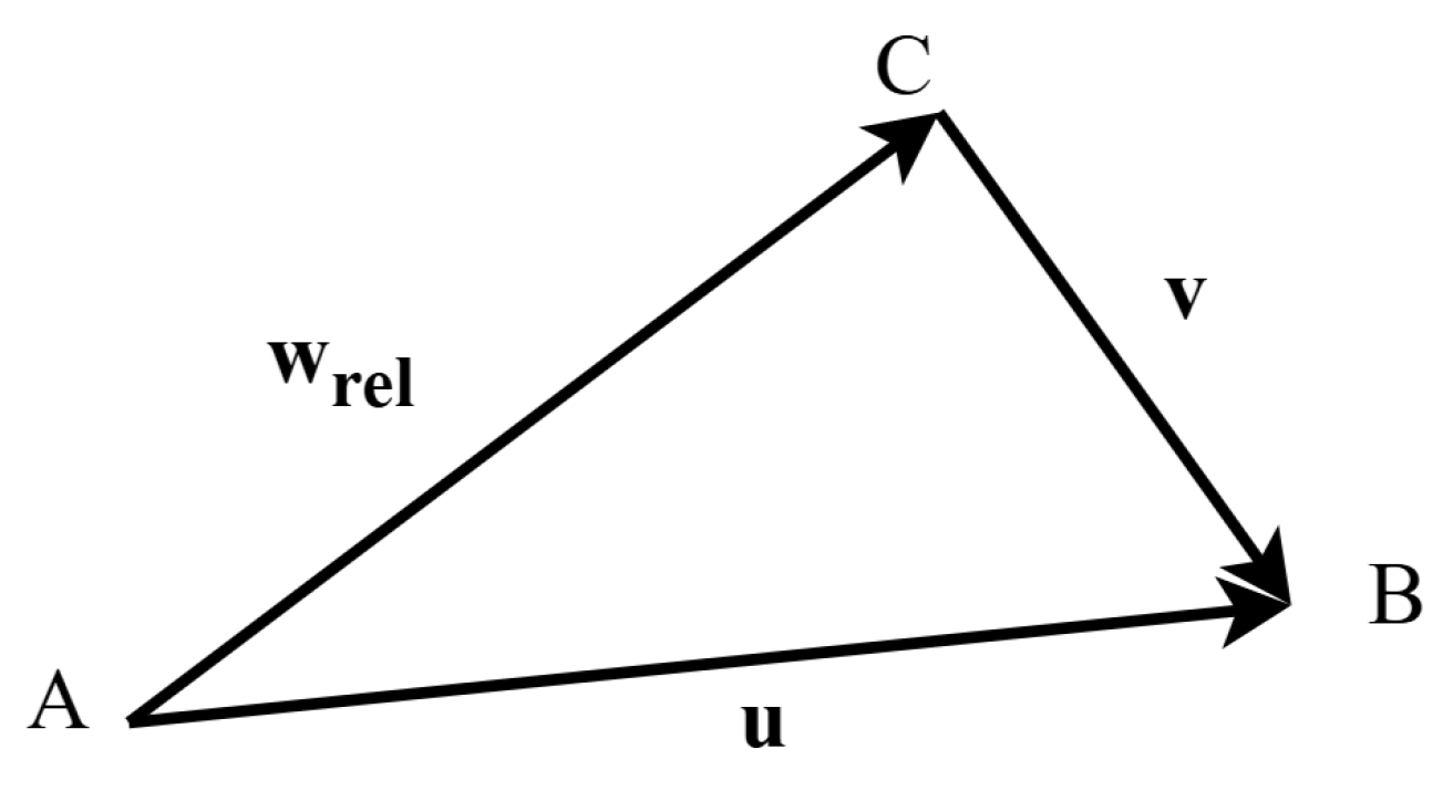
Airflow reconstruction using a moving UAV requires relating three velocity quantities: the wind velocity $\mathbf{u}$ expressed in the inertial frame, the UAV ground-relative velocity $\mathbf{v}$ in the same frame, and the velocity of the air ${\mathbf{w}}_{\mathrm{rel}}$ relative to the UAV. Their relation is given by

$${\mathbf{w}}_{\mathrm{rel}}=\mathbf{u}-\mathbf{v}.$$

(1)

This relation also illustrates the distinction between the different flow descriptions introduced above. For a stationary Eulerian measurement platform, $\mathbf{v}=0$, and therefore the measured relative airflow corresponds directly to the ambient airflow velocity. For an ideal Lagrangian tracer, $\mathbf{v}=\mathbf{u}$ and consequently ${\mathbf{w}}_{\mathrm{rel}}=0$. In the present semi-Lagrangian case, the UAV follows the airflow only partially, such that $\mathbf{v}\ne \mathbf{u}$ and a non-zero relative velocity remains.

Rearranging Equation (1) gives

$$\mathbf{u}={\mathbf{w}}_{\mathrm{rel}}+\mathbf{v}.$$

(2)

The geometric interpretation of this relative velocity relation is illustrated in Figure 1.

In the present study, the two velocity contributions required for the reconstruction are obtained from two independent measurement systems: the body-axis relative airflow component $w_B$ is measured along the UAV body axis using a Pitot tube-based differential pressure sensor, while the UAV ground-relative velocity $\mathbf{v}$ is derived from a camera-based stereo-vision system via 3D trajectory reconstruction. Equation (2) therefore provides the basis for estimating the wind velocity $\mathbf{u}$. The UAV ground-relative velocity represents the drift motion of the platform, whereas the relative air velocity accounts for the remaining slip between the moving UAV and the surrounding airflow.

The present feasibility study focuses on the streamwise wind component along the global $x_G$-axis. Taking the $x_G$-component of Equation (2) gives

$$u_x=w_x+v_x.$$

(3)

Here, $u_x$ is the wind velocity along the global flow direction, $w_x$ is the streamwise component of the relative wind velocity, and $v_x$ is the UAV drift velocity along the same axis. Thus, $v_x$ alone does not represent the full streamwise wind velocity unless the UAV behaves as an ideal flow tracer. The relative wind contribution $w_x$ is required to compensate for the slip between the UAV drift motion and the surrounding airflow.

Equation (3) is the streamwise component of the general vector relation and does not itself require the lateral and vertical velocity components to vanish. However, the present single-axis Pitot tube measures only the relative airflow component along its body-fixed sensing axis. Recovering $w_x$ from this measurement therefore requires the additional assumption that the relative airflow is predominantly aligned with the global $x_G$-axis. The effect of possible lateral and vertical relative flow components on this reconstruction is considered explicitly in Section 2.3. For complex atmospheric wind fields with changing flow directions or significant three-dimensional velocity components, the complete vector relation would have to be considered together with multi-directional relative flow sensing.

2.3. Coordinate Frames and Rotation Transformations

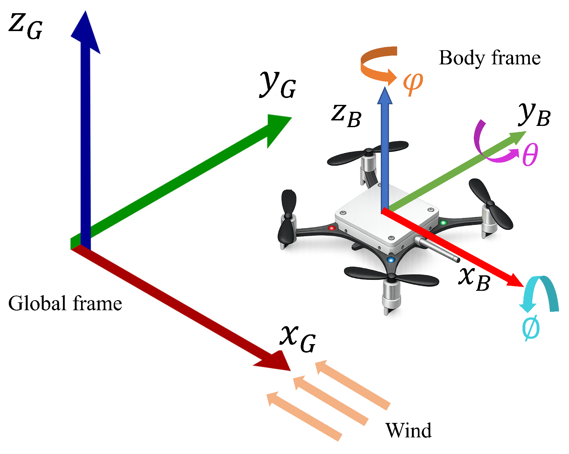
Wind reconstruction requires that all velocity quantities in Equation (2) are expressed in a common reference frame. A coordinate transformation is therefore required. In this study, two coordinate frames are employed: a global inertial frame G and a UAV body-fixed frame B.

The global frame G is defined such that its $x_G$-axis is aligned with the reverse direction of the measured airflow. The body frame B is rigidly attached to the UAV, with its $x_B$-axis pointing forward along the nose of the vehicle and coinciding with the sensing axis of the Pitot tube. The UAV orientation with respect to the global frame is described by the roll $\varphi$, pitch $\theta$, and yaw $\psi$ Euler angles. The global and body-fixed coordinate frames and the corresponding Euler angles are illustrated in Figure 2.

In the general three-dimensional case, the relative airflow vector in the global frame can be expressed as

$${\mathbf{w}}_{\mathrm{rel}}^G={\left[\begin{array}{ccc}{w}_x& w_y& w_z\end{array}\right]}^T,$$

(4)

where $w_x$, $w_y$, and $w_z$ denote the streamwise, lateral, and vertical components of the relative airflow, respectively.

The UAV orientation relative to the global frame is described by the body-to-global rotation matrix $R_B^G(\varphi ,\theta ,\psi )$, using the standard 3–2–1 (yaw–pitch–roll) Euler angle convention [24]. The relative wind vector expressed in the body-fixed frame is therefore obtained as

$${\mathbf{w}}_{\mathrm{rel}}^B={\left(R_B^G(\varphi ,\theta ,\psi )\right)}^T{\mathbf{w}}_{\mathrm{rel}}^G.$$

(5)

Accordingly, the component of the relative airflow along the Pitot tube sensing axis $x_B$ is

$${\left({\mathbf{w}}_{\mathrm{rel}}^B\right)}_x={\left(R_B^G\right)}_{11}{w}_x+{\left(R_B^G\right)}_{21}{w}_y+{\left(R_B^G\right)}_{31}{w}_z.$$

(6)

In the adopted sign convention, positive ${\left({\mathbf{w}}_{\mathrm{rel}}^B\right)}_x$ corresponds to airflow entering the forward-facing Pitot tube, whereas the relative airflow vector is directed opposite to the positive $x_B$-axis.

Thus, for the general case, the measured body-axis relative airflow is

$$w_B=-\left[{\left(R_B^G\right)}_{11}{w}_x+{\left(R_B^G\right)}_{21}{w}_y+{\left(R_B^G\right)}_{31}{w}_z\right].$$

(7)

Equation (7) shows that lateral and vertical relative flow components $w_y$ and $w_z$ can contribute to the single-axis Pitot measurement when the sensing axis is not perfectly aligned with the global streamwise direction. Such relative flow components can result from lateral or vertical components of the fan-generated airflow and also from lateral or vertical UAV motion. Furthermore, variations in UAV attitude modify the corresponding projection coefficients in Equation (7).

For the present feasibility study, the relative airflow within the investigated measurement volume is assumed to be predominantly aligned with the global $x_G$-axis. Therefore, the lateral and vertical relative flow components are neglected and the relative airflow vector is approximated as

$${\mathbf{w}}_{\mathrm{rel}}^G\approx {\left[\begin{array}{ccc}{w}_x& 0& 0\end{array}\right]}^T.$$

(8)

Under this assumption, the component along the body-fixed $x_B$-axis reduces to

$${\left({\mathbf{w}}_{\mathrm{rel}}^B\right)}_x={\left(R_B^G(\varphi ,\theta ,\psi )\right)}_{11}{w}_x.$$

(9)

The measured body-axis relative airflow is consequently

$$w_B=-{\left(R_B^G(\varphi ,\theta ,\psi )\right)}_{11}{w}_x.$$

(10)

Solving Equation (10) for the global projected relative wind component gives

$$w_x=-{\displaystyle \frac{w_B}{{\left(R_B^G(\varphi ,\theta ,\psi )\right)}_{11}}}.$$

(11)

where ${\left(R_B^G\right)}_{11}$ denotes the element in the first row and first column of the rotation matrix. For the chosen Euler angle convention, this term simplifies to

$${\left(R_B^G(\varphi ,\theta ,\psi )\right)}_{11}=\cos \theta \cos \psi .$$

(12)

Consequently, the projected relative wind component is obtained as

$$w_x=-{\displaystyle \frac{w_B}{\cos \theta \cos \psi }}.$$

(13)

The correction in Equation (13) depends on the alignment between the Pitot tube sensing axis and the global streamwise direction. For $\theta =\psi =0$, the sensing axis is aligned with the global $x_G$-axis and the correction factor is unity. As the angular deviation increases, $\cos \theta \cos \psi$ decreases, and the Pitot tube measures a smaller axial component of the streamwise relative airflow. Therefore, maintaining approximate alignment of the UAV with the nominal flow direction is important for the present single-axis measurement approach.

If $w_y$ or $w_z$ are non-zero, however, applying Equation (11) gives an estimated streamwise component

$${\widehat{w}}_x=w_x+{\displaystyle \frac{{\left(R_B^G\right)}_{21}}{{\left(R_B^G\right)}_{11}}}{w}_y+{\displaystyle \frac{{\left(R_B^G\right)}_{31}}{{\left(R_B^G\right)}_{11}}}{w}_z,$$

(14)

so that the projected lateral and vertical components are interpreted as part of the streamwise relative wind velocity. They can therefore introduce an additional deviation and variability in the reconstructed $u_x$. The present single-axis approach should consequently be interpreted as a streamwise reconstruction under predominantly unidirectional relative flow conditions. Directionally varying or fully three-dimensional airflow would require multi-directional relative flow sensing together with the complete vector formulation.

2.4. Direct Sensing of the Relative Wind Velocity

The relative wind velocity along the UAV body axis $x_B$ is obtained using a Pitot tube-based differential pressure sensor. The sensor measures the pressure difference

$$\Delta p=p_0-p_s,$$

(15)

between the stagnation pressure at the probe inlet and the static pressure at the lateral ports.

Under incompressible flow conditions, this differential pressure corresponds to the dynamic pressure of the airflow. According to Bernoulli’s equation [10], the magnitude of the axial relative wind velocity is given by

$$|w_B|=\sqrt{{\displaystyle \frac{2|\Delta p|}{\rho }}},$$

(16)

where $\rho$ denotes the air density, obtained from the ideal gas law using the onboard temperature measurement.

Since the differential pressure signal can take both positive and negative values during flight, a signed velocity estimate is introduced by assigning the sign of $\Delta p$ to the square-root expression,

$$w_B=\mathrm{sgn}(\Delta p)\sqrt{{\displaystyle \frac{2|\Delta p|}{\rho }}}.$$

(17)

The signed extension is used for preprocessing purposes and should not be interpreted as a physical measurement of reverse flow.

The resulting $w_B$ represents the axial relative airflow velocity measured along the UAV body-fixed $x_B$-axis. Under the predominantly streamwise relative flow assumption introduced in Section 2.3, the corresponding streamwise component $w_x$ in the global frame is obtained using Equation (11).

2.5. Global UAV Velocity from Stereo-Vision Tracking

For the wind reconstruction, the UAV ground-relative velocity $\mathbf{v}$ must be known in the global inertial frame G. The stereo-vision system provides a time-resolved estimate of the UAV position,

$${\mathbf{P}}^G\left(t\right)=\left[\begin{array}{c}{x}_G\left(t\right)\\ y_G\left(t\right)\\ z_G\left(t\right)\end{array}\right],$$

which describes the UAV trajectory in the global inertial frame. The corresponding velocity vector is defined as the time derivative of this trajectory,

$$\mathbf{v}\left(t\right)={\displaystyle \frac{d{\mathbf{P}}^G\left(t\right)}{dt}}.$$

(18)

Since the vision system provides discrete position measurements at timestamps $t_k$, the UAV’s ground-relative velocity is obtained from the finite difference in the reconstructed trajectory. Because this study considers a unidirectional flow aligned with the global $x_G$-axis, only the axial component of the UAV motion is required. The drift velocity is therefore computed as

$$v_x={\displaystyle \frac{x_G\left(t_k\right)-x_G\left(t_{k-1}\right)}{t_k-t_{k-1}}}.$$

(19)

Together, the quantities obtained from Section 2.4 and Section 2.5 provide the two terms required for the one-dimensional relative velocity relation in Equation (3). The direct sensing method yields the relative wind component $w_x$ expressed in the global frame, while the stereo-vision system provides the UAV drift velocity $v_x$ along the same axis.

3. Experimental Setup

3.1. General Setup and Experimental Procedure

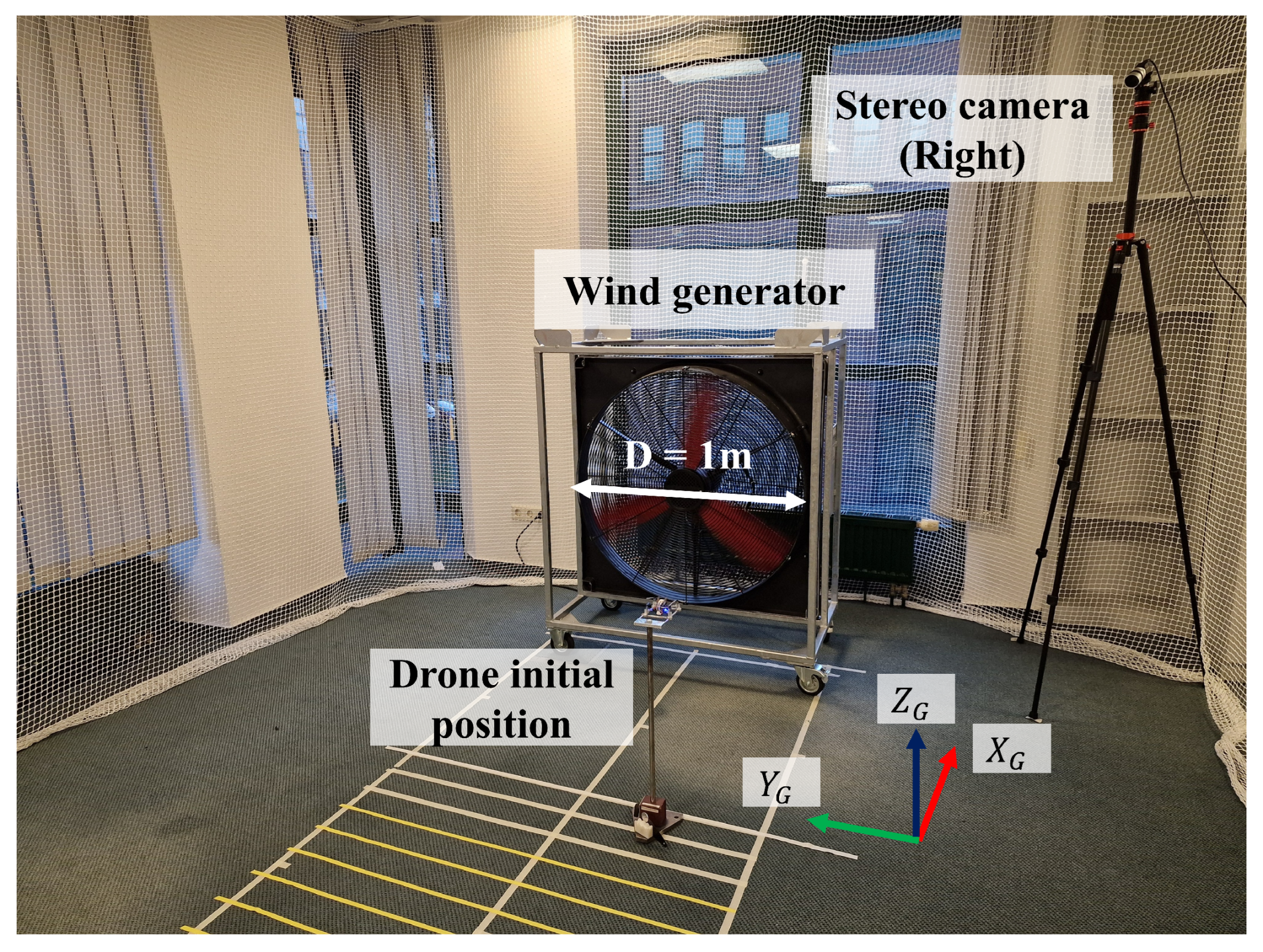
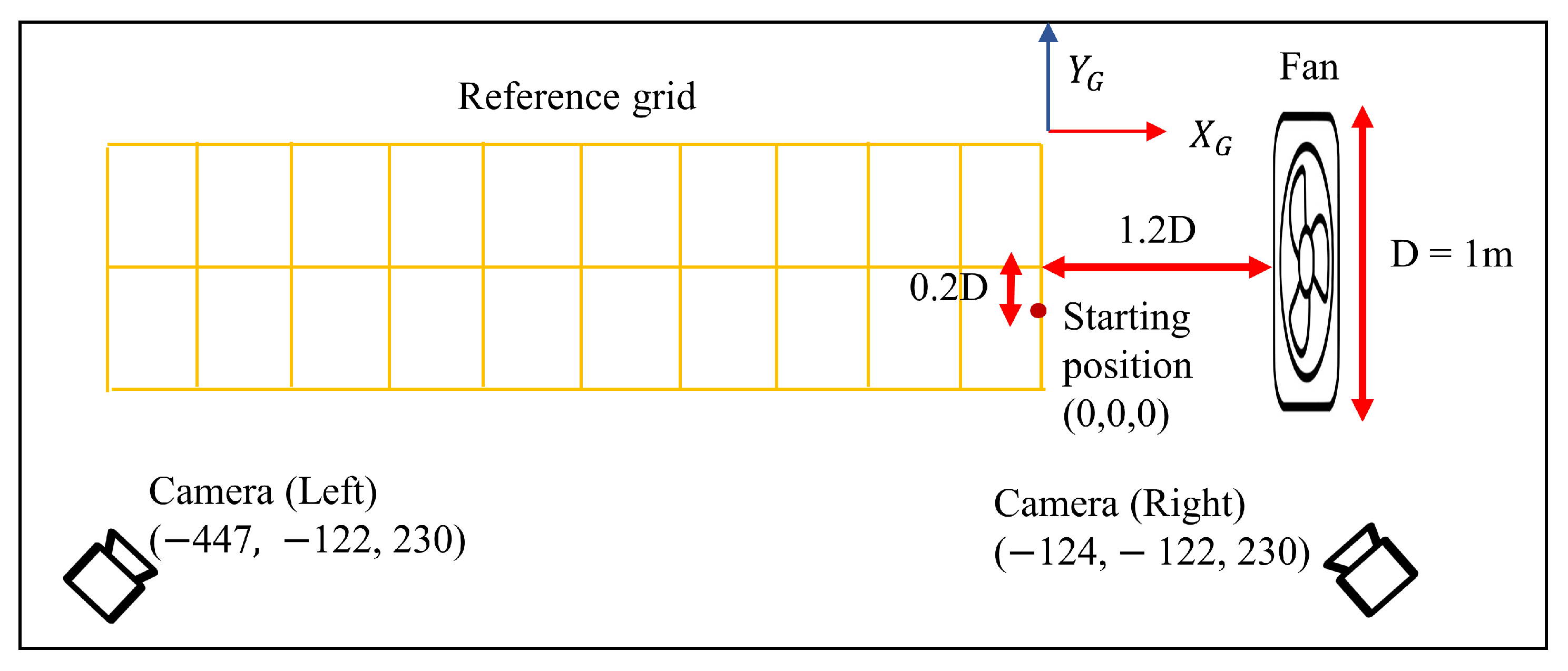
The setup of the experimental environment, including the wind machine, the stereo cameras, and the global coordinate system, is shown in Figure 3. All the experiments are conducted in a netted indoor test area with dimensions of $4\times 6\times 3{\mathrm{m}}^3$. Airflow is generated using a three-blade axial wind machine, TTW 20000 from Trotec, which is positioned to produce a flow predominantly along the global streamwise axis, opposite to the positive $x_G$-axis defined in Section 2. The wind machine has a circular outlet with a radius of approximately $1\mathrm{m}$ and a maximum rated outlet airspeed of $8.8\mathrm{m}/\mathrm{s}$. The speed controller of the wind machine allows the outlet velocity to be varied.

The generated airflow is not perfectly uniform across the outlet cross-section. Higher wind speeds are observed near the central region of the radius and lower speeds toward the outer radius. This behavior results in a radially varying, bell-shaped speed distribution. Depending on the measurement location and the setting of the speed regulator within the flow field, peak wind speeds of up to approximately $10\mathrm{m}/\mathrm{s}$ are achievable. Despite these variations, the airflow within the measurement volume is assumed to be predominantly one-directional in order to be consistent with the one-dimensional wind reconstruction approach adopted in this study. To ensure repeatable initial conditions, the UAV is placed on a dedicated take-off platform for each experiment. The platform is designed to introduce minimal disturbance to the airflow. It is positioned $1.2\mathrm{m}$ downstream from the wind machine and $0.2\mathrm{m}$ offset from the center of the wind outlet. The platform height is $0.52\mathrm{m}$ above the floor. This is the starting location of the UAV for all measurements. The selected position ensures that the UAV experiences a drift after take-off, even at the lowest wind speed setting.

For each predefined wind machine speed setting, 30 independent drift experiments are conducted with the same initial position. During the experiments, onboard sensor data and stereo-vision data are recorded simultaneously. The onboard measurements include differential pressure, temperature, and UAV attitude (roll $\varphi$, pitch $\theta$, and yaw $\psi$), which are logged with a sampling rate of $50\mathrm{Hz}$. Simultaneously, image streams from the stereo-vision system are recorded at 24 frames per second. All data are stored and processed offline.

3.2. UAV Setup and Relative Wind Measurement

The experiments are conducted using a miniaturized Crazyflie 2.1+ quadrotor UAV from Bitcraze, which is an open-source development platform. The UAV has a mass of approximately $29\mathrm{g}$ in its standard configuration and a motor-to-motor dimension of $92\times 92\times 29{\mathrm{mm}}^3$. It is equipped with an STM32F405 main application microcontroller and an onboard inertial measurement unit (IMU), which provides attitude-related measurements required for flight stabilization and coordinate transformation. Without additional payload, the UAV achieves a flight time of approximately $7\min$. The UAV is controlled from a host computer via a Crazyradio 2 radio link. Both the manufacturer-provided client software and a Python-based application programming interface (API) (cflib, version 0.1.33) are available for command and data handling. During the experiments, the Python API is used to enable flexible control and synchronized data logging.

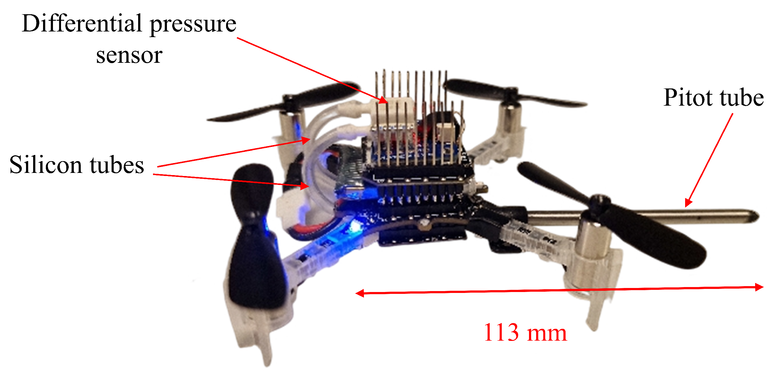
In order to measure $w_x$ during semi-Lagrangian drift operation, a Pitot tube-based differential pressure sensor (Matek Digital Airspeed Sensor, ASPD-4525) is integrated into the UAV. It provides a digital I²C interface, which allows integration into the onboard firmware. The sensor is capable of unidirectional airspeed measurements and is mounted such that its measurement axis is aligned with the UAV body-fixed $x_B$-axis. A straight Pitot tube with a length of 8 cm is connected to the sensor using short silicone tubes. The probe tip is thereby displaced from the UAV body and rotors in order to reduce the influence of rotor-induced flow and body-induced flow distortion at the sensing location. This arrangement follows the general principle of positioning airflow probes away from the multirotor wake and vehicle body [12]. However, the selected probe position does not guarantee complete elimination of rotor-induced disturbances. The specific sensor is selected because it satisfies the payload and integration requirements of the Crazyflie platform. The sensor board has a mass of approximately $3.5\mathrm{g}$, and the combined mass of the sensor, Pitot tube, tubing, and mounting components is approximately $5\mathrm{g}$. Since the Crazyflie can carry only a maximum payload of approximately $15\mathrm{g}$, the sensor payload has to remain below this limit to be operated in the semi-Lagrangian drift mode. Including all sensor attachments, the total UAV mass during the experiments is approximately $35\mathrm{g}$. In addition to the payload constraint, the sensor selection considered the electrical integration, power consumption, and measurement range. The Matek ASPD-4525 provides a digital I²C interface compatible with the onboard electronics and has a working current of approximately $5\mathrm{mA}$. The underlying TE 4525DO-DS5AI001DP differential pressure sensor has a manufacturer-specified accuracy of $\pm 0.25\%$ of the pressure span. These characteristics, together with the low sensor mass, enabled direct integration into the miniaturized UAV while maintaining the low total mass required for semi-Lagrangian drift operation. No comparative experimental evaluation of alternative airflow sensors was performed in the present study. Therefore, the selection of the Matek ASPD-4525 should be understood as a practical choice that satisfied the payload, electrical-interface, power-consumption, and integration requirements of the present feasibility study, rather than as the optimal solution for semi-Lagrangian airflow measurements.

However, the selected sensor is not optimized for very low airspeed measurements. According to the manufacturer’s specifications, it supports airspeed measurements up to $100\mathrm{m}/\mathrm{s}$, which is much higher than the velocities investigated here. The wind machine provides outlet velocities up to approximately $8.8\mathrm{m}/\mathrm{s}$, and during semi-Lagrangian operation, the UAV partially follows the flow. Therefore, the relative airspeed at the Pitot tube is most of the time lower than the absolute wind speed in the surroundings, and the sensor therefore operates close to the lower end of its measurement range during the drift. Since airspeed is obtained from the square-root relation between differential pressure and velocity, small pressure fluctuations at low relative airspeeds can cause comparatively large fluctuations in the converted velocity signal. This behavior is also consistent with the manufacturer’s information that comparatively large airspeed fluctuations can occur near zero differential pressure, whereas the same pressure variations have a smaller influence on the calculated velocity at higher airspeeds. Therefore, increased variability of the relative wind estimate is expected under the present operating conditions. The sensor should therefore be considered as a lightweight, low-cost, and UAV-compatible solution for feasibility testing, rather than as a high-precision anemometer in the low-speed range. The zero-flow calibration described below corrects the mean pressure offset, but does not remove the short-term fluctuations of the pressure signal near zero differential pressure. These fluctuations are therefore characterized experimentally and included in the uncertainty analysis.

The differential pressure signal is logged together with temperature and UAV attitude data. Prior to the drift measurements, a zero-flow calibration is performed in a still-air enclosure using the final sensor, Pitot tube, tubing, and mounting configuration. The mean pressure value over a $30\mathrm{s}$ interval under no-wind conditions is used as a constant bias and subtracted from all subsequent measurements to reduce offsets introduced by the complete sensing configuration. The same stationary recording is also used to characterize the short-term repeatability of the pressure measurement. After bias correction and filtering, the differential pressure signal exhibits a standard deviation of $2.17\mathrm{Pa}$, which is adopted as the experimental standard uncertainty $u(\Delta p)$ in the subsequent uncertainty propagation. The bias-corrected signal is then filtered using a first-order exponential low-pass filter. For the drift measurements, different time constants are evaluated, and a value of $0.2\mathrm{s}$ is selected as a compromise between noise suppression and temporal responsiveness. Due to the linear nature of the low-pass filter, bias removal can equivalently be applied before or after filtering without affecting the steady-state signal. The air density is then estimated from the measured temperature assuming constant ambient pressure and a representative indoor relative humidity of $40\%$. The filtered differential pressure signal is converted to relative wind velocity using Equation (17). The recorded UAV attitude is later used for the coordinate transformation described in Section 2.3 to express the measured relative wind velocity in the global frame, resulting in $w_x$, which forms the first contribution to the wind reconstruction. Because the onboard sensor data are recorded at $50\mathrm{Hz}$ and the stereo-vision system operates at $24\mathrm{Hz}$, the two measurement streams do not provide samples at identical timestamps. To combine the two velocity contributions sample by sample, the stereo-derived drift velocity $v_x$ is temporally interpolated to the timestamps of the differential pressure measurements. The resulting synchronized values of $v_x$ and $w_x$ are then combined according to Equation (3) to obtain the reconstructed streamwise wind velocity $u_x$.

3.3. UAV Steering, Tracking and Drift Velocity Estimation

In this study, the UAV is operated with open-loop thrust, meaning that the motor thrust is fixed during flight and no automatic altitude control is used. As a result, the UAV is unable to correct vertical motion by itself. When wind is applied, the aerodynamic forces acting on the UAV change with wind speed. Therefore, the same thrust value does not result in the same vertical behavior under different wind speeds. On the other hand, the UAV is released from an initial height of 0.52 m above the floor. Since the altitude is not regulated, mismatches between thrust and the required lift can lead to a loss of altitude that can quickly result in ground contact. To ensure a sufficient observation time for measurements, the thrust must be chosen to avoid altitude descent immediately after release. Therefore, the thrust value is calibrated for each wind speed setting. The thrust command is determined iteratively for each wind setting. Starting from an initial command, the thrust is adjusted between successive test flights until the UAV can leave the take-off platform and undergo a sufficiently long downstream drift without an immediate loss of altitude or ground contact. Once a suitable value is identified for a given wind setting, the same constant thrust command is used for all drift experiments at that setting. The selected thrusts are capable of maintaining the UAV’s height approximately constant during the initial drift phase.

The thrust calibration is performed for three distinct wind speed settings of the wind machine, which correspond to $25\%$, $50\%$ and $75\%$ of the maximum output of the wind machine speed controller. The relative definition of the wind machine’s speed levels is adopted because a single representative wind speed value cannot be assigned since the flow field varies within the measurement volume. The calibrated thrust values for each wind speed setting are summarized in

Table 1. Calibrated thrust values used for Crazyflie framework as 16-bit integer to drift the UAV at different wind speed settings.

Wind Speed Setting (%)	Thrust Command (16-Bit Integer)
25	56,000
50	58,000
75	62,000

.

The use of a setting-dependent thrust means that the UAV does not behave as a purely passive tracer. This is consistent with the semi-Lagrangian concept adopted in this study: the UAV remains an actively powered platform whose translational motion is influenced by the airflow, but its velocity is not assumed to equal the local wind velocity. During each run, the selected thrust command remains constant and no active position control is applied along the streamwise direction. The difference between the resulting UAV drift velocity and the surrounding airflow is therefore analyzed through the measured relative wind contribution $w_x$ in Equation (3). However, the different thrust levels can modify the UAV dynamics and the rotor-induced flow around the Pitot tube location. The influence of thrust on the local probe flow is not characterized independently and therefore remains a limitation of the present implementation.

During the experiments, the UAV is released into the airflow by applying the calibrated thrust for the corresponding wind speed setting and then operated in semi-Lagrangian mode. No active position control is applied along the flow direction, and no altitude control is used. However, in order to prevent unintended rotations of the UAV, an attitude control is applied by correcting the rotations to zero. This provides a smooth drift behavior and preserves alignment with the global flow direction, i.e., the $x_G$-axis.

In order to estimate the UAV drift velocity $v_x$, a stereo-vision system is developed to estimate the three-dimensional position of the UAV during the drift. Two synchronized industrial cameras are mounted on tripods along the long side of the experimental area, as illustrated in Figure 4. The cameras are placed to have a sufficiently overlapping field of view covering the maximum possible measurement volume. Since stereo depth estimation accuracy decreases with increasing object distance, the long side camera placement is chosen to minimize the distance between the UAV and the cameras throughout the flight. This configuration reduces depth uncertainty and improves triangulation accuracy, particularly for large displacements along the flow direction. Both cameras are equipped with lenses of $12.5\mathrm{mm}$ focal length, which provide a suitable field of view and spatial resolution to detect the UAV over a sufficient measurement area.

Prior to the experiments, the stereo-vision system is calibrated to determine the intrinsic parameters of each camera as well as the relative pose between them. Calibration is performed using a planar chessboard target. The UAV is tracked using an onboard LED. For each synchronized image pair, the LED is detected independently in the left and right camera image using intensity-based segmentation. A morphological top-hat filter enhances small bright structures, followed by adaptive thresholding and area filtering to isolate the LED. The centroid of the selected blob defines the image coordinates in both views.

Using the calibrated intrinsic and extrinsic stereo parameters, the corresponding image points are triangulated to obtain the three-dimensional LED position. The position estimates are initially expressed in the stereo camera coordinate system and then transformed into the global reference frame defined in Section 2.3. From the transformed trajectory, the global position $x_G\left(t\right)$ is extracted. The initial UAV position at release is chosen as the origin of this global frame, with the UAV body axes aligned with the coordinate system’s axes at take-off. The drift velocity $v_x$ is computed from the temporal evolution of the position $x_G\left(t\right)$ using the formula introduced in Equation (19). The resulting $v_x$ represents the UAV ground-relative velocity component along the global flow direction and provides the second contribution to the wind reconstruction. The drift velocity $v_x$ obtained from stereo tracking and the relative wind component $w_x$ derived from the differential pressure measurements are finally combined according to Equation (3) to reconstruct the wind velocity $u_x$.

3.4. Reference Wind Speed Measurement

Reference wind speed measurements are carried out using a hot-wire anemometer (Testo 440) equipped with a telescopic hot-wire probe and an integrated temperature sensor. The sensor measures air velocity in the range of approximately $0.1$–$30\mathrm{m}/\mathrm{s}$ with a specified accuracy of $\pm 0.03\mathrm{m}/\mathrm{s}+4\%$ of the measured value.

The anemometer is used to measure the airflow generated by the wind machine in the measurement area. Since the flow produced by the fan is not homogeneous across the measurement volume, a reference measurement grid is defined to capture spatial variations in wind speed. A vertical grid consisting of $7\times 7$ measurement points with a uniform spacing of $15\mathrm{cm}$ is defined perpendicular to the incoming flow direction. Wind speed measurements are taken at each grid intersection by positioning the hot-wire probe at the corresponding location and aligning it with the direction of the incoming flow.

The grid measurements are repeated at downstream distances of $1\mathrm{m}$, $2\mathrm{m}$, and $3\mathrm{m}$ from the wind machine for each of the three wind speed settings defined in Table 1. At each grid location, the measured wind speed is time-averaged over a period of $30\mathrm{s}$. The resulting reference measurements are used to construct a spatial wind speed grid, which serves as a baseline for comparison with the UAV-based wind reconstruction. In order to determine the corresponding measurement position of the UAV, the camera-derived 3D position of the UAV LED is corrected for the displacement between the LED and the Pitot tube sensor tip, see Figure 5. The reference grid is acquired separately from the UAV drift experiments and therefore does not provide a simultaneous instantaneous wind measurement. Instead, the $30\mathrm{s}$ time-averaged measurements define a spatial mean reference field for each wind setting. During comparison with the UAV reconstruction, this spatial field is interpolated to the instantaneous Pitot tube position along the reconstructed UAV trajectory. Consequently, the reference value associated with each UAV sample represents the local time-averaged wind velocity at the corresponding spatial position rather than the instantaneous airflow present during that particular drift experiment.

4. Results and Discussion

The results are presented following the one-dimensional wind reconstruction model introduced in Equation (3). According to this relation, the reconstructed streamwise wind velocity $u_x$ is obtained by combining the projected relative wind velocity $w_x$ with the UAV drift velocity $v_x$. Although $w_x$ appears first in the reconstruction equation, $v_x$ is discussed first because it represents the semi-Lagrangian motion of the UAV and establishes the repeatability of the drifting measurement platform. The behavior of the UAV-mounted relative wind estimate $w_x$ is evaluated as the second contribution to the reconstruction. The combined wind reconstruction is then compared with the reference wind measurements. Finally, the measurement uncertainty and achievable velocity range are discussed, together with the main factors limiting the reconstruction accuracy.

4.1. Estimation and Repeatability of the UAV Drift Velocity $v_x$

Drift experiments are conducted at three wind settings corresponding to 25%, 50%, and 75% of the maximum output of the wind machine. During all experiments, the UAV is released from the same initial position and allowed to drift with the airflow under the constant thrust command selected for the corresponding wind setting. The first $0.2\mathrm{s}$ after release is excluded from the dataset to remove the initial transient associated with the take-off phase. All reported quantities in this subsection therefore refer to the valid drift window beginning at $t=0.2\mathrm{s}$.

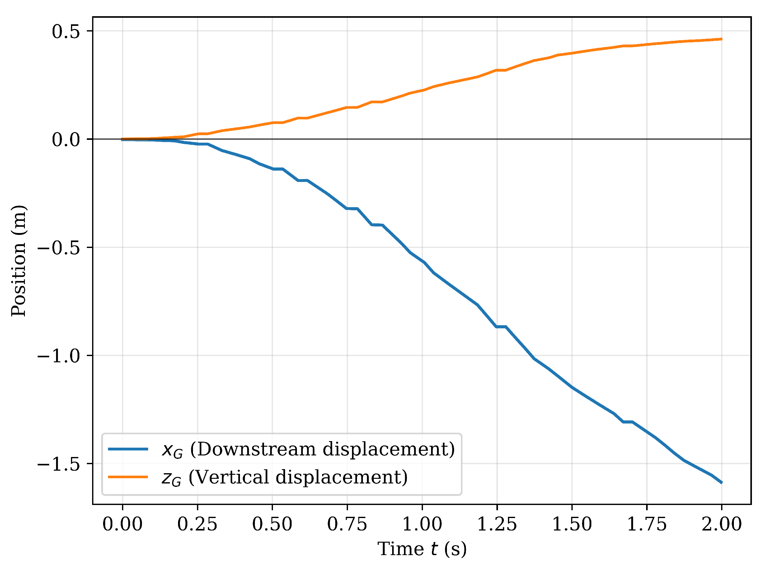
Figure 6 shows a representative global trajectory of the UAV for the 25% wind setting. The downstream position $x_G\left(t\right)$ decreases continuously, indicating convection of the UAV along the airflow direction. After the initial transient associated with the take-off phase, the trajectory becomes approximately linear, suggesting that the UAV motion is primarily governed by the surrounding flow during the drift phase. In this regime, the UAV exhibits flow-driven downstream translation under the applied constant thrust, consistent with the semi-Lagrangian concept introduced in Section 2. At the same time, the vertical position $z_G\left(t\right)$ increases gradually during the flight, which reflects the open-loop thrust configuration used in the experiments.

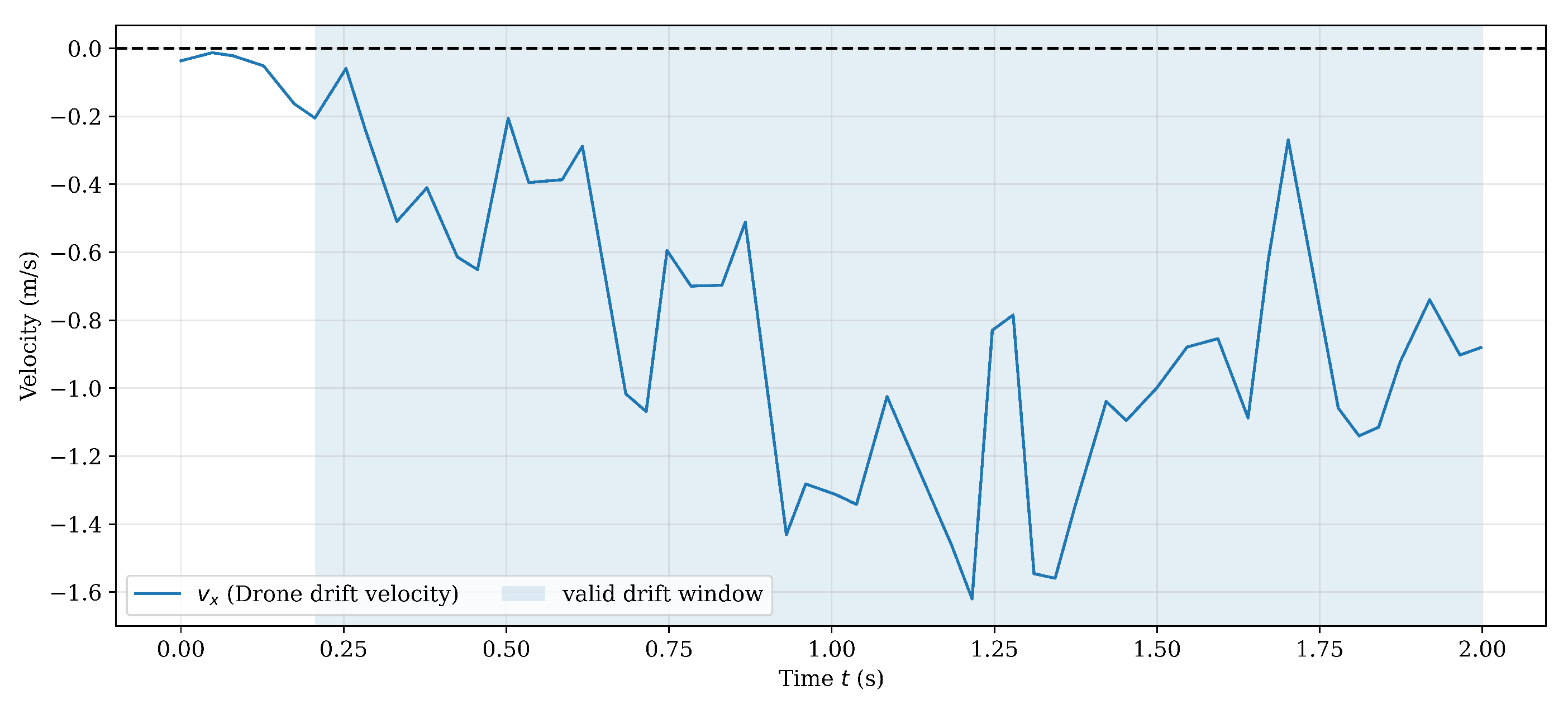
The corresponding streamwise drift velocity $v_x\left(t\right)$ obtained from the temporal derivative of the trajectory according to Equation (19) is shown in Figure 7. After excluding the take-off phase, the velocity initially increases in magnitude and then approaches a nearly constant negative value, corresponding to downstream motion along the defined global $x_G$-axis. This behavior indicates that the UAV rapidly reaches a steady drift velocity during the valid drift window used for the statistical analysis.

To evaluate the repeatability of the semi-Lagrangian drift behavior, statistical measures of the drift duration and drift velocity are computed across all runs for each wind setting. The results are summarized in

Table 2. Drift statistics for the three wind settings. Values correspond to the median and interquartile range (IQR) across runs.

Wind Setting	N Runs	${\mathit{T}}_{\mathbf{drift}}$ (s)	Median ${\mathit{v}}_{\mathit{x}}$ (m/s)
25%	30	1.89 (1.80–1.99)	$-0.86$ ($-0.89$–$-0.77$)
50%	30	1.03 (0.93–1.14)	$-1.43$ ($-1.60$–$-1.22$)
75%	30	0.83 (0.72–1.14)	$-1.65$ ($-1.87$–$-1.50$)

. Increasing the wind setting leads to an increase in the magnitude of the drift velocity while the drift duration decreases. This behavior is expected because stronger aerodynamic forcing acts on the UAV at higher wind speeds, which accelerates the vehicle more rapidly downstream and reduces the time spent within the measurement volume. Except for these changes, the interquartile ranges (IQRs) remain relatively compact across all operating conditions, indicating repeatable drift behavior.

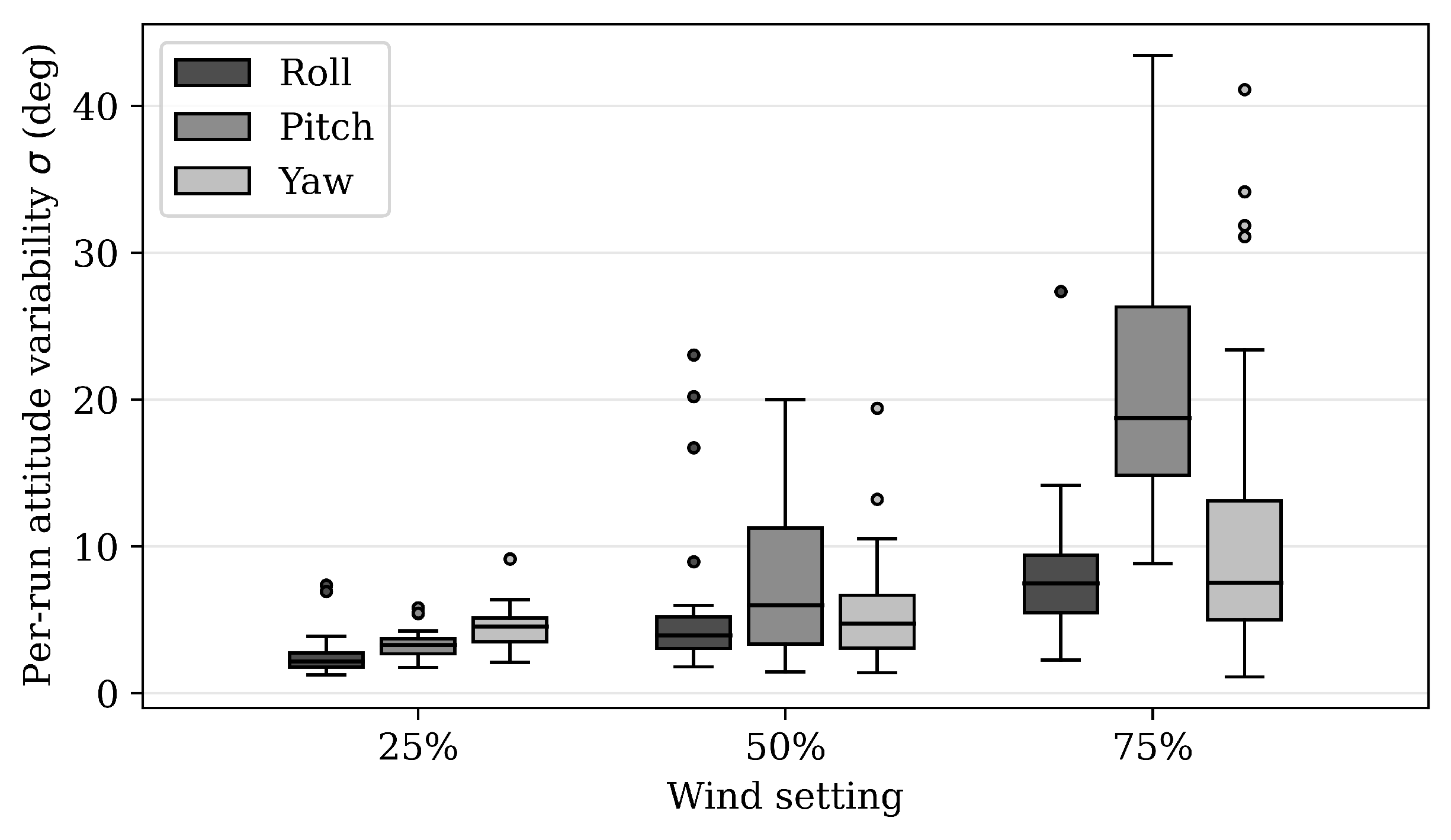
In addition to the translational motion, the UAV attitude is relevant for using the drifting platform as a relative wind measurement system. During the drift experiments, although the UAV is allowed to translate with the airflow, its orientation is stabilized. This control is necessary because the relative wind velocity is measured along the UAV body-fixed $x_B$-axis using the UAV-mounted Pitot tube. To obtain the largest axial relative flow component at the probe, the probe axis should remain approximately aligned with the incoming flow. Figure 8 shows the per-run attitude variability for roll, pitch, and yaw across the three wind settings, expressed as the standard deviation of the Euler angles within the valid drift window. At the lowest wind setting, the UAV maintains comparatively stable alignment with the global flow direction, with angular variations remaining within a few degrees. As the wind setting increases, the attitude variability increases, most noticeably for pitch. This attitude behavior is relevant for the subsequent estimation of $w_x$, because the body-axis relative wind measurement is used to recover the projected relative wind component in the global frame according to Equation (11).

The results demonstrate that the UAV can be operated in a repeatable semi-Lagrangian drift mode under the investigated laboratory conditions. The stereo-vision system provides a consistent estimate of the streamwise drift velocity $v_x$. The observed increase in $|v_x|$ from $0.86\mathrm{m}/\mathrm{s}$ to $1.65\mathrm{m}/\mathrm{s}$ confirms that the UAV motion responds systematically to the imposed wind setting. The attitude results further show that the UAV can maintain approximate alignment with the nominal flow direction at the lowest wind setting, whereas this alignment becomes more difficult at higher wind settings. Therefore, $v_x$ provides a repeatable drift velocity contribution for the wind reconstruction in Equation (3), while the attitude behavior is relevant for the subsequent estimation of the projected relative wind velocity $w_x$.

4.2. Estimation and Behavior of the Relative Wind Velocity $w_x$

After evaluating the UAV drift velocity $v_x$, the relative wind velocity $w_x$ is analyzed as the second velocity contribution in Equation (3). The body-axis relative wind velocity is obtained from the differential pressure measurement according to Section 2.4. It is then transformed into the global streamwise direction using Equation (11). Therefore, $w_x$ represents the relative airflow contribution measured from the moving UAV and expressed in the same coordinate frame as the stereo-derived drift velocity $v_x$.

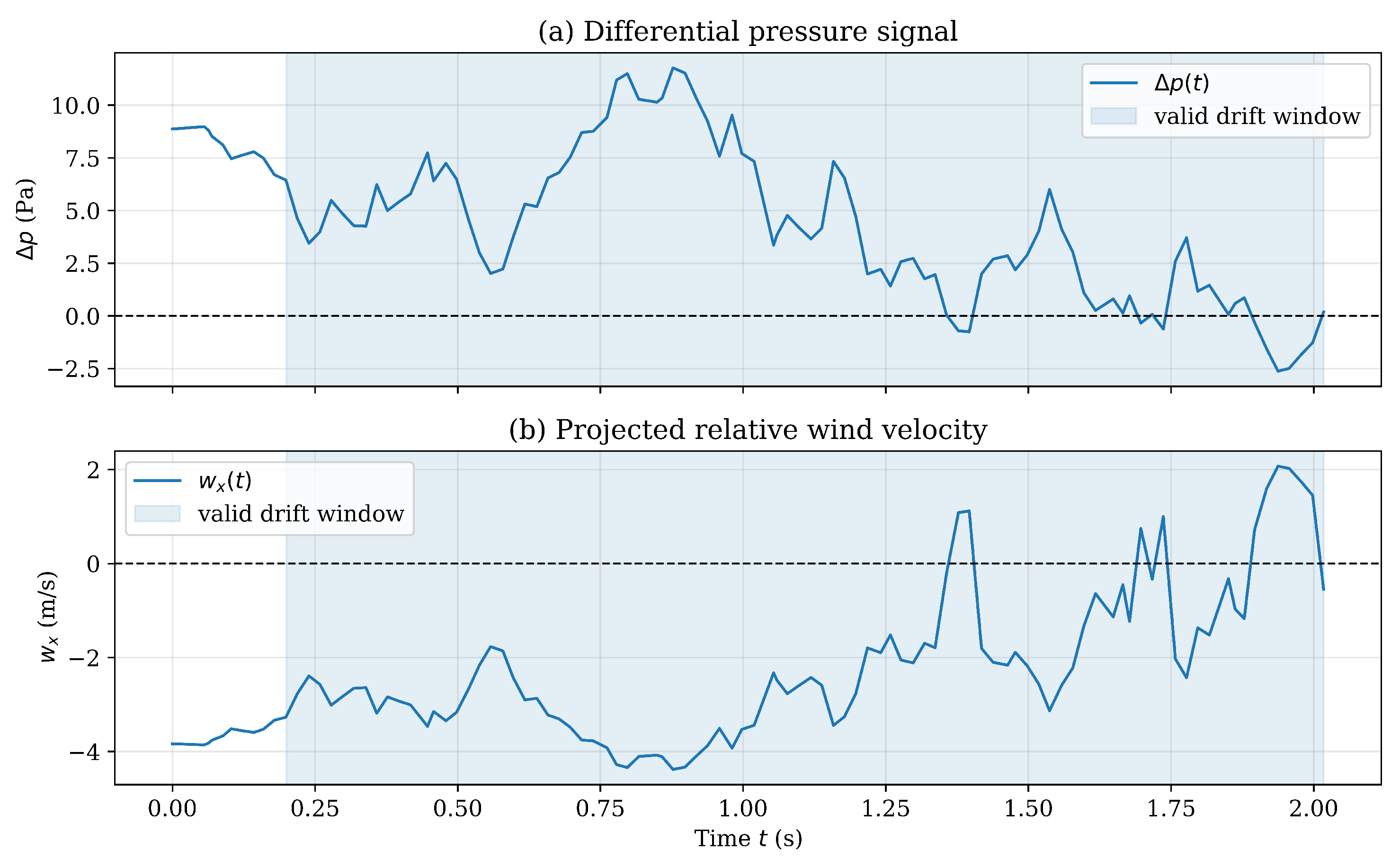
Figure 9 shows a representative drift run for the 25% wind setting. Panel (a) shows the measured differential pressure signal $\Delta p\left(t\right)$, while panel (b) shows the corresponding projected relative wind velocity $w_x\left(t\right)$. During most of the valid drift window, $w_x\left(t\right)$ remains in the negative velocity range, which is consistent with the defined global streamwise direction for this representative run. However, compared with the streamwise drift velocity $v_x\left(t\right)$ discussed in Section 4.1, the projected relative wind velocity shows stronger temporal fluctuations. Short intervals with positive $w_x$ values are also observed. Since the global flow direction does not reverse during the experiment, these positive values are not interpreted as reverse-flow velocities, but as non-physical sign behavior of the pressure-derived relative wind estimate.

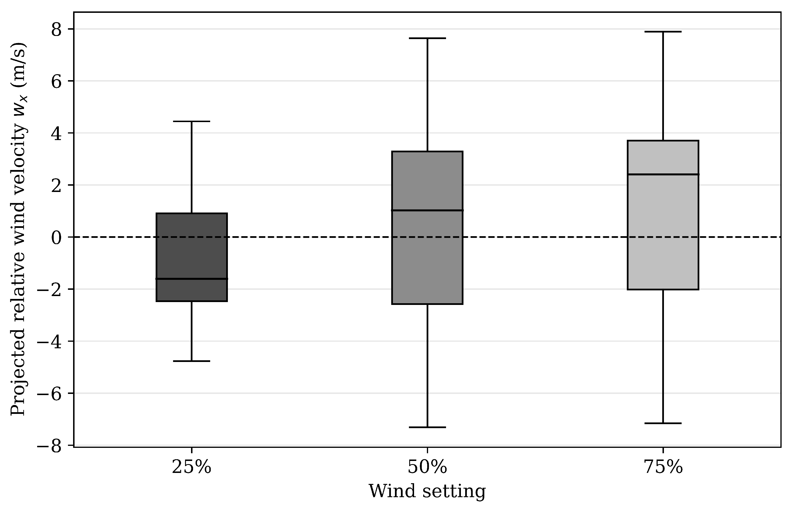
The sample-wise distributions of $w_x$ within the valid drift windows are shown in Figure 10 for the three wind settings. In contrast to the run-wise drift statistics reported in Section 4.1, the distribution of $w_x$ is evaluated sample-wise because temporal fluctuations of the relative wind estimate directly affect the reconstruction of $u_x$. The boxplots show a broad spread for all operating conditions. At the 25% wind setting, the median of $w_x$ is located in the negative velocity range at $-1.60\mathrm{m}/\mathrm{s}$. At the 50% and 75% wind settings, the medians shift toward positive values of $1.02\mathrm{m}/\mathrm{s}$ and $2.41\mathrm{m}/\mathrm{s}$, respectively. At the same time, the interquartile ranges remain large, extending from $-2.47$ to $0.91\mathrm{m}/\mathrm{s}$ at 25%, from $-2.58$ to $3.28\mathrm{m}/\mathrm{s}$ at 50%, and from $-2.02$ to $3.70\mathrm{m}/\mathrm{s}$ at 75%. This shows that the initial pressure-derived $w_x$ estimate contains strong sample-wise variability during drift operation.

For the chosen coordinate definition, the projected relative wind velocity is expected to remain mainly in the negative streamwise direction during drift. Therefore, the shift in the distributions toward positive values, especially at the higher wind settings, indicates an increasing occurrence of non-physical sign behavior. This behavior is associated with negative differential pressure samples, which appear as positive $w_x$ values after the signed velocity conversion and projection into the global frame. Under the low differential pressure conditions of semi-Lagrangian drift, small pressure variations caused by sensor noise and residual offset can change the sign of the measured differential pressure. The sensitivity of the selected sensor in the low-speed range further amplifies the resulting velocity variability, but it is not interpreted as the main cause of the sign changes. In addition, attitude variations affect the relation between the body-axis measurement and the projected relative wind component through Equation (11). Rotor-induced flow can be another possible contribution to the observed variability of $w_x$, since the Pitot tube measures the local airflow at the probe position. Although the probe is displaced from the rotor region, residual wake interaction and local flow distortion around the UAV can still influence the pressure measurement. The effect can also vary with UAV attitude and rotor operating condition during the drift. Therefore, rotor-induced disturbances may contribute to the fluctuations observed in the pressure-derived relative wind estimate. However, the rotor-induced flow field at the probe position is not measured separately in the present experiments. Its contribution therefore cannot be quantitatively separated from sensor noise, residual pressure offset, and other local flow disturbances.

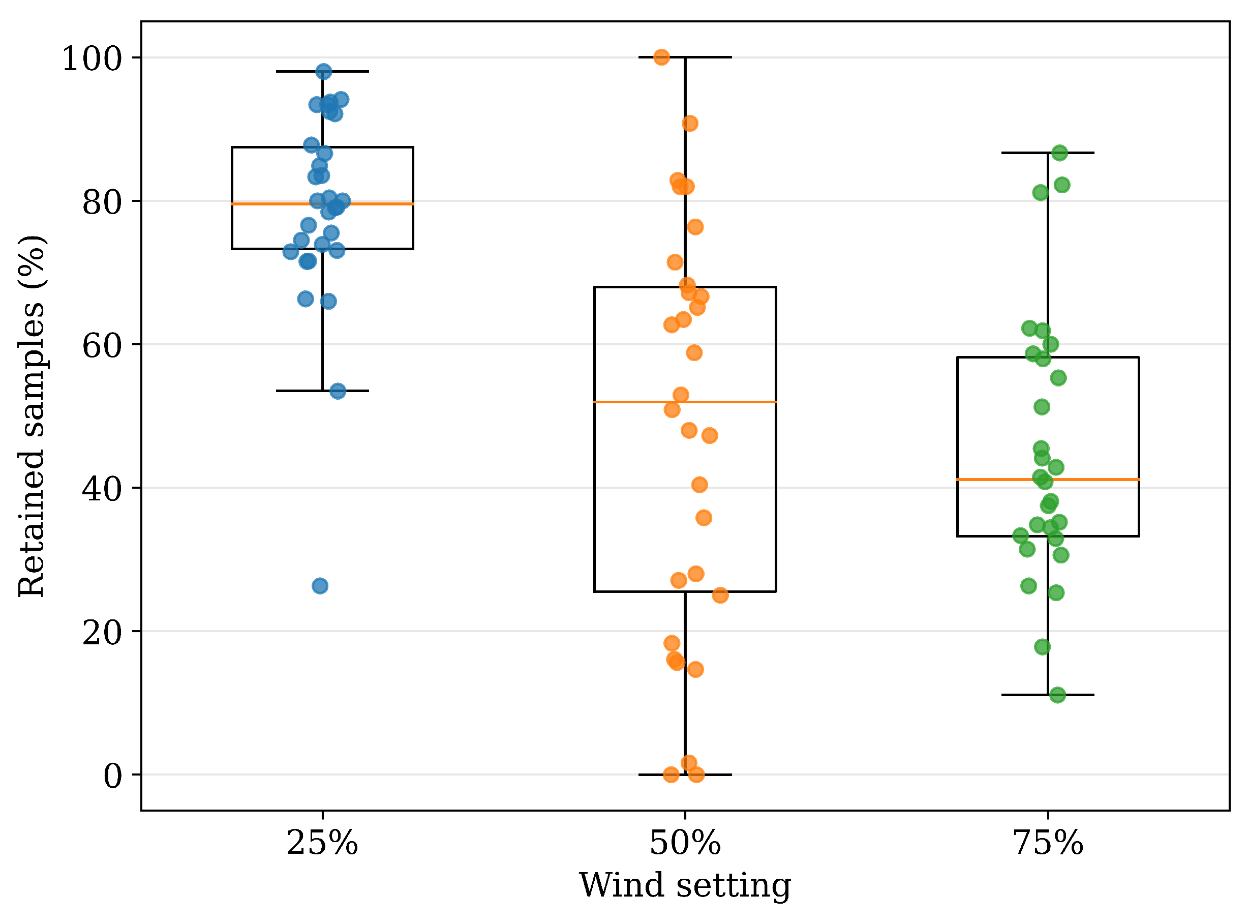
For the subsequent wind reconstruction, sign-based filtering is applied based on the known direction of the imposed unidirectional airflow. Sign-inconsistent samples are identified after bias correction and low-pass filtering of the pressure signal, but before pressure-to-velocity conversion. A short interval is defined as an adjacent run of at most five samples, corresponding to 0.10 s at the 50 Hz sampling rate. These short negative-pressure gaps are replaced by linear interpolation of the low-pass pressure between the nearest valid samples on either side. Longer gaps, or gaps not bounded by valid samples, are retained as invalid values and excluded from subsequent velocity reconstruction. The retained and rejected fractions therefore refer to the final sample set after this preprocessing procedure. To quantify the effect of the filtering, the retained fraction is evaluated separately for each drift run, as shown in Figure 11, while the corresponding pooled retained and rejected fractions are summarized in

Table 3. Pooled fractions of retained and rejected pressure-derived relative wind samples after applying the sign-based filtering.

Wind Setting	${\mathit{N}}_{\mathbf{runs}}$	Retained Samples (%)	Rejected Samples (%)
25%	30	79.0	21.0
50%	30	48.3	51.7
75%	30	44.3	55.7

. The run-wise results show a comparatively high and consistent retained fraction at the lowest wind setting, whereas the distribution becomes broader at the intermediate setting and the retained fraction generally decreases at the higher settings. The pooled results show the same trend, with the rejected fraction exceeding the retained fraction at the 50% and 75% settings. In addition, two runs at the 50% setting contain no retained samples, and consequently no filtered wind reconstruction can be obtained for these runs. These results indicate that the availability of valid pressure-derived relative wind measurements becomes a limitation of the present sensing configuration as the wind setting increases.

The present sign-based filtering relies on prior knowledge of the imposed unidirectional flow direction. If the true flow direction is unknown or changes during operation, a sign change cannot be interpreted unambiguously as an invalid measurement. In such conditions, the present single-axis Pitot tube configuration would require an independent flow-direction estimate or multi-directional relative flow sensing. The applied filtering is therefore specific to the controlled feasibility experiments considered here. The analysis shows that the pressure-derived relative wind estimate is the more variable contribution in Equation (3). While $v_x$ provides a repeatable estimate of the UAV motion across runs, the initial $w_x$ estimate shows temporal fluctuations, broad sample-wise distributions, and intermittent non-physical sign behavior during drift. These observations indicate that not all pressure-derived relative wind samples are suitable for quantitative wind reconstruction under the investigated unidirectional inflow condition. Thus, the pressure-derived relative wind contribution has a stronger influence on the sample-wise variability of the reconstructed wind velocity than the stereo-derived drift velocity.

4.3. Wind Reconstruction Performance

After analyzing the two velocity contributions separately, the reconstructed wind velocity is evaluated by combining the UAV drift velocity $v_x$ with the projected relative wind velocity $w_x$ according to Equation (3). As shown in Section 4.2, the initial pressure-derived relative wind estimate contains samples with non-physical sign behavior under the investigated unidirectional flow condition. To evaluate the influence of these samples on the reconstruction, the reconstruction performance is first determined using all pressure-derived samples and is then evaluated after applying the sign-based filtering described in Section 4.2. For the subsequent reconstruction and uncertainty analysis, only pressure-derived relative wind samples retained by the sign-based filtering are used. These samples are converted into the projected relative wind velocity $w_x$ and combined with the corresponding stereo-derived drift velocity $v_x$. The reconstructed streamwise wind velocity $u_x$ is then compared with the spatially interpolated, time-averaged reference wind velocity $u_{\mathrm{ref}}$ obtained from the separately acquired hot-wire reference field. The reconstruction performance and the resulting measurement uncertainty are then used to assess the achievable measurement range of the proposed approach.

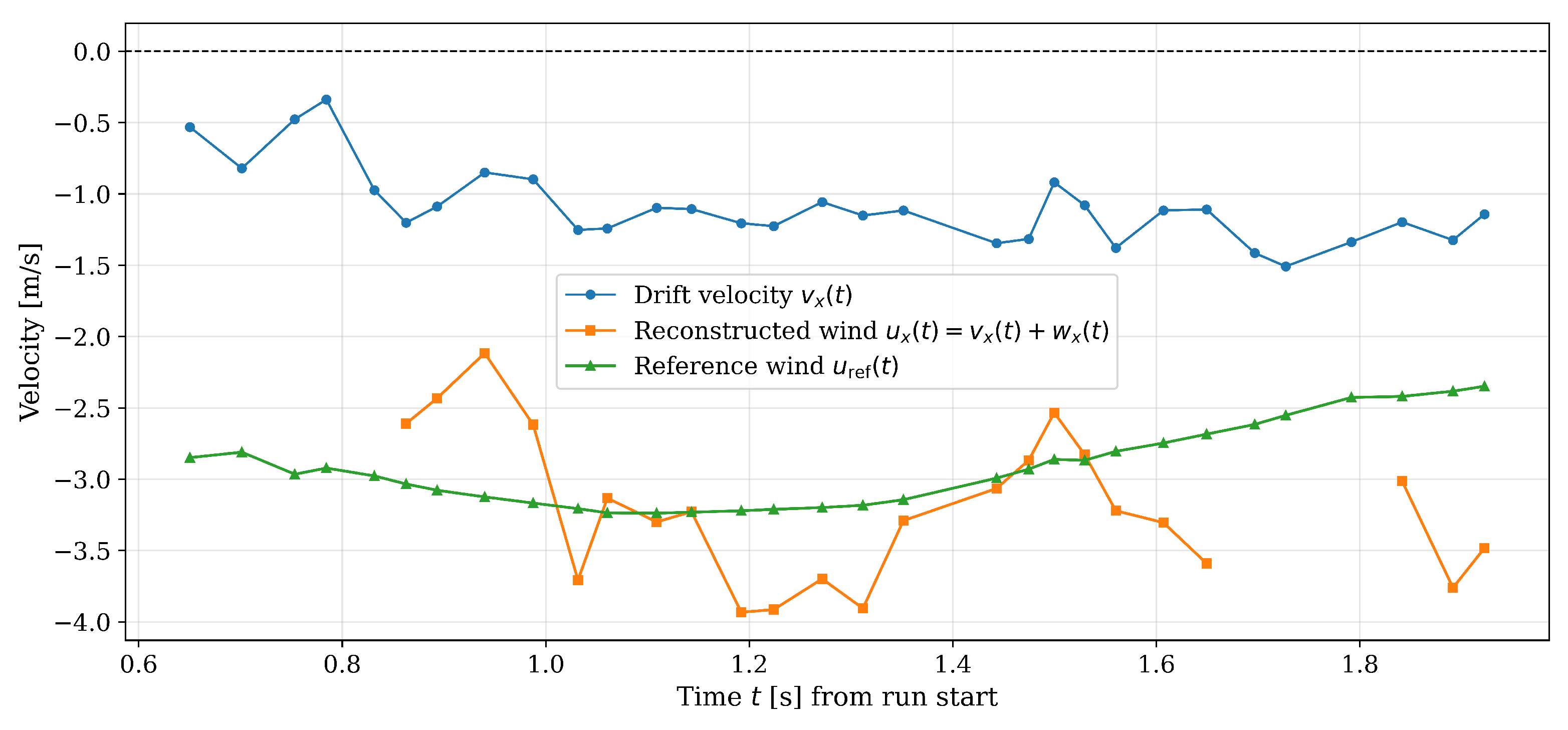
A representative run for the 25% wind setting is shown in Figure 12. The reconstructed wind velocity $u_x\left(t\right)$ is shifted closer to the reference wind velocity $u_{\mathrm{ref}}\left(t\right)$ than the drift velocity $v_x\left(t\right)$ alone. This illustrates the role of the onboard relative wind measurement in converting the observed UAV drift motion into an airflow velocity estimate. The gaps in the reconstructed curve indicate time instances at which pressure-derived relative wind samples are excluded due to non-physical sign behavior. The reconstructed signal still shows sample-wise variations, which are mainly associated with the relative wind contribution, as already observed from the behavior of $w_x$ in Section 4.2. The same qualitative behavior is observed for the 50% and 75% wind settings.

To quantify the reconstruction performance relative to the reference field, the sample-wise reconstruction-to-reference deviation is evaluated. Since the reference field is acquired separately from the UAV experiments and represents a time-averaged spatial wind field, the term reconstruction error is used in this study to denote this reconstruction-to-reference deviation rather than the error relative to a simultaneous instantaneous reference measurement.

The reconstruction error is defined as

$$e\left(t\right)=u_x\left(t\right)-u_{\mathrm{ref}}\left(t\right),$$

(20)

where $u_{\mathrm{ref}}\left(t\right)$ denotes the value obtained by spatially interpolating the time-averaged reference field to the instantaneous Pitot tube position along the UAV trajectory. The reconstruction error therefore includes contributions from the UAV-based reconstruction as well as temporal differences between the separately acquired reference field and the airflow during the UAV experiment, spatial interpolation effects, and reference measurement uncertainty. These contributions cannot be separated using the present experimental data. Consequently, the reported reconstruction error should not be interpreted as a direct measure of instantaneous reconstruction accuracy.

The quantitative influence of the sign-based filtering is first evaluated using these reconstruction-to-reference statistics.

Table 4. Comparison of reconstruction performance before and after applying the sign-based filtering to the pressure-derived relative wind samples.

Wind Setting	Processing	Mean Error (m/s)	Std. Dev. (m/s)	RMSE (m/s)
25%	Before filtering	0.69	1.75	1.88
	After filtering	$-0.17$	0.88	0.89
50%	Before filtering	2.47	3.12	3.97
	After filtering	$-0.39$	1.26	1.31
75%	Before filtering	3.52	2.66	4.41
	After filtering	0.01	1.22	1.21

compares the reconstruction performance before and after applying the filtering. Before filtering, the mean reconstruction error, its variability, and the RMSE increase with increasing wind setting. After filtering, the mean errors are closer to zero and both the standard deviation and RMSE are reduced for all three operating conditions. The reduction is particularly noticeable at the 50% and 75% wind settings, which is consistent with the larger fraction of sign-inconsistent pressure-derived samples observed at these settings. The improvement in the reconstruction statistics after filtering must be considered together with the reduction in available pressure-derived samples reported in Section 4.2. In particular, the lower reconstruction errors at the higher wind settings are obtained from a reduced subset of the measured data. Thus, the sign-based filtering improves the reconstructed wind estimate under the present known unidirectional flow condition, but with reduced measurement availability.

The reconstruction error is computed for the retained reconstruction samples within the drift window across all runs. Following application of the sign-based filtering, the mean reconstruction errors are $-0.17$ m/s, $-0.39$ m/s, and $0.01$ m/s for the 25%, 50%, and 75% wind settings, respectively. The corresponding standard deviations are $0.88$ m/s, $1.26$ m/s, and $1.22$ m/s, which are clearly larger than the mean errors. The corresponding MAE values are $0.74$ m/s, $1.05$ m/s, and $0.96$ m/s, respectively. The comparatively small mean errors indicate no considerable average deviation from the time-averaged reference field, whereas the larger standard deviations demonstrate substantial sample-wise reconstruction-to-reference variability.

The sample-wise reconstruction error is further reflected by the RMSE values of $0.89$ m/s, $1.31$ m/s, and $1.21$ m/s for the 25%, 50%, and 75% wind settings, respectively. The proposed system is implemented on a miniaturized UAV with a total mass of approximately $35\mathrm{g}$, which is substantially smaller than the platforms used in earlier wind measurement studies. Neumann et al. [5] reported a wind-estimation RMSE range of approximately $0.36$–$0.60\mathrm{m}/\mathrm{s}$ using a $1.3\mathrm{kg}$ quadcopter, and Kistner et al. [7] demonstrated airflow measurements with a $0.645\mathrm{kg}$ UAV while reporting RMSE values of $0.2$–$0.6\mathrm{m}/\mathrm{s}$. Although the present RMSE values are not lower than the previously reported values, they are achieved on a substantially lighter platform and under a semi-Lagrangian drift configuration. The results therefore demonstrate the feasibility of the reconstruction concept under the investigated conditions, while also showing that the present pressure-based sensing implementation remains a major limitation of the achievable measurement performance.

When interpreting the mean reconstruction errors, the uncertainty of the reference wind measurement must also be taken into account. The instrument uncertainty of the hot-wire anemometer is specified by

$$U_{\mathrm{inst}}=0.03\mathrm{m}/\mathrm{s}+0.04\left|u_{\mathrm{ref}}\right|,$$

(21)

where $u_{\mathrm{ref}}$ denotes the reference wind velocity in m/s. In the present experiments, the total reference wind uncertainty also includes the spatial variability of the reference grid used for interpolation to the UAV trajectory. This contribution is estimated as the standard deviation of the neighboring reference-grid values surrounding the instantaneous Pitot tube position. The resulting reference wind uncertainties are $0.30\pm 0.11$ m/s, $0.45\pm 0.18$ m/s, and $0.67\pm 0.30$ m/s for the 25%, 50%, and 75% wind settings, respectively. Since these values are of the same order of magnitude as the mean reconstruction errors, the observed mean deviations cannot be conclusively attributed to a systematic bias of the UAV-based reconstruction alone. The quantified reference uncertainty accounts for the specified instrument uncertainty and the local spatial variability of the reference field. Temporal differences between the separately acquired reference measurements and the airflow during the UAV experiments cannot be quantified from the available data.

After establishing the effect of the sign-based filtering, the benefit of combining the UAV drift velocity with the relative wind measurement is evaluated quantitatively. To determine whether the improvement observed in the representative example is also obtained across the experiments, a paired run-level comparison is performed using the retained reconstruction samples. For each run, the drift-only estimate and the combined reconstruction are compared with the same spatially interpolated reference values using exactly the same retained timestamps. Thus, samples for which no valid pressure-derived reconstruction is available are also excluded from the drift-only comparison.

For this comparison, the reconstruction-to-reference deviation is given by Equation (20), while the corresponding drift-to-reference deviation is defined as

$$e_v\left(t\right)=v_x\left(t\right)-u_{\mathrm{ref}}\left(t\right).$$

(22)

For each run, the RMSE is calculated separately from the reconstruction-to-reference and drift-to-reference deviations using identical retained samples, resulting in one drift-only RMSE and one reconstruction RMSE per run. The values reported in

Table 5. Run-wise comparison of the drift-only estimate and the combined wind reconstruction using identical retained samples. RMSE values are reported as mean ± standard deviation across the paired runs.

Wind Setting	Drift-Only RMSE (m/s)	Reconstruction RMSE (m/s)	Runs with Lower RMSE
25%	$1.95\pm 0.15$	$0.87\pm 0.21$	100.0%
50%	$2.51\pm 0.58$	$1.15\pm 0.34$	100.0%
75%	$2.77\pm 0.91$	$1.27\pm 0.81$	87.5%

represent the mean and standard deviation of these run-wise RMSE values. The paired comparison shows a clear reduction in run-wise RMSE when the relative wind contribution is included. The combined reconstruction provides a lower RMSE for all paired runs at the 25% and 50% wind settings and for $87.5\%$ of the paired runs at the 75% setting. As summarized in Table 5, the mean run-wise RMSE of the combined reconstruction is consistently lower than that of the drift-only estimate for all three operating conditions. These results quantitatively confirm that for the retained pressure-derived samples, combining the UAV drift velocity with the relative wind measurement generally improves the wind estimate compared with using the drift velocity alone.

Together, the reconstruction results show that the semi-Lagrangian velocity relation can be used to combine UAV motion sensing and onboard relative wind sensing into a streamwise wind estimate. The paired run-level comparison demonstrates that inclusion of the retained relative wind contribution generally reduces the deviation from the reference field compared with the UAV drift velocity alone.

Having quantified the reconstruction-to-reference performance, the measurement uncertainty of the UAV-based reconstruction is evaluated separately from the observed reconstruction-error variability. The observed variability of $w_x$ is therefore not treated directly as measurement uncertainty. Instead, the uncertainty is propagated from the individual input quantities of the reconstruction model. By combining Equations (3), (13) and (17), the measurement model can be written as

$$u_x=v_x-{\displaystyle \frac{\mathrm{sgn}(\Delta p)\sqrt{2|\Delta p|/\rho }}{\cos \theta \cos \psi }}.$$

(23)

The input quantities considered in the uncertainty propagation are therefore the stereo-derived drift velocity $v_x$, differential pressure $\Delta p$, air density $\rho$, pitch $\theta$, and yaw $\psi$. Their standard uncertainties are evaluated independently before being propagated through Equation (23). For the differential pressure contribution, the experimentally determined standard uncertainty $u(\Delta p)=2.17\mathrm{Pa}$ from the stationary zero-flow characterization described in Section 3.2 is used. The air-density contribution is evaluated from the variability of the density calculated under the same stable conditions using the temperature-based density model employed during the drift experiments, resulting in $u\left(\rho \right)=3.25\times {10}^{-4}\mathrm{kg}/{\mathrm{m}}^3$. Since an independent attitude-characterization experiment is not available, the pitch and yaw uncertainties are estimated as Type-B standard uncertainties based on reported attitude-estimation performance for the Crazyflie 2.1 platform. A recent study reports attitude RMSE values below approximately $3°$ under slow and medium flight conditions. Accordingly, conservative standard uncertainties of $u\left(\theta \right)=3°$ and $u\left(\psi \right)=3°$ are adopted for the present uncertainty propagation [25].

The stereo-vision contribution is characterized using two experiments. First, the stationary LED experiment provides a baseline estimate of the short-term tracking repeatability. The reconstructed streamwise position exhibits a standard deviation of $0.053\mathrm{mm}$, corresponding to a velocity contribution of approximately $0.0018\mathrm{m}/\mathrm{s}$ for the measured frame interval. Second, the spatial reconstruction performance is assessed by manually translating the UAV through ten nominal $100\mathrm{mm}$ displacements along the streamwise direction. The standard deviation of the displacement error is $1.95\mathrm{mm}$, corresponding to a relative spatial reconstruction contribution of $1.95\%$. This translation experiment does not constitute a dynamic velocity calibration, but provides an additional characterization of the spatial stereo-reconstruction performance beyond the stationary-target test. The stereo-derived velocity uncertainty used in the propagation is therefore expressed as

$$u(v_x,t)=\sqrt{u_{v_x,\mathrm{static}}^2+{\left(r_x\left|v_x\left(t\right)\right|\right)}^2},$$

(24)

where $u_{v_x,\mathrm{static}}=0.0018\mathrm{m}/\mathrm{s}$ and $r_x=0.0195$ denotes the relative spatial contribution obtained from the translation experiment.

A first-order uncertainty propagation is applied to Equation (23). The corresponding combined standard uncertainty is given by

$$u_c^2\left(u_x\right)={\left({\displaystyle \frac{\partial u_x}{\partial v_x}}u\left(v_x\right)\right)}^2+{\left({\displaystyle \frac{\partial u_x}{\partial \Delta p}}u(\Delta p)\right)}^2+{\left({\displaystyle \frac{\partial u_x}{\partial \rho }}u\left(\rho \right)\right)}^2+{\left({\displaystyle \frac{\partial u_x}{\partial \theta }}u\left(\theta \right)\right)}^2+{\left({\displaystyle \frac{\partial u_x}{\partial \psi }}u\left(\psi \right)\right)}^2.$$

(25)

The magnitudes of the sensitivity coefficients used for the sample-wise propagation are

$$\left|{\displaystyle \frac{\partial u_x}{\partial v_x}}\right|=1,$$

(26)

$$\left|{\displaystyle \frac{\partial u_x}{\partial \Delta p}}\right|={\displaystyle \frac{1}{\rho |w_B\left|\right|\cos \theta \cos \psi |}},$$

(27)

$$\left|{\displaystyle \frac{\partial u_x}{\partial \rho }}\right|={\displaystyle \frac{|w_x|}{2\rho }},$$

(28)

$$\left|{\displaystyle \frac{\partial u_x}{\partial \theta }}\right|= |w_x\tan \theta |,$$

(29)

$$\left|{\displaystyle \frac{\partial u_x}{\partial \psi }}\right|= |w_x\tan \psi |.$$

(30)

The individual measurement-error contributions are treated as uncorrelated because the drift velocity, differential pressure, density, and attitude quantities originate from separate measurement or estimation inputs. This assumption concerns the error contributions in the measurement model and does not imply statistical independence of the physical quantities $v_x$ and $w_x$ during drift.

Equation (25) is evaluated separately for every retained reconstruction sample. The sample-wise uncertainty contributions are first averaged within each run, and the values reported for each wind setting correspond to the mean and standard deviation of these run-wise mean uncertainties. The resulting uncertainty budget is summarized in

Table 6. Propagated standard uncertainty budget for the reconstructed streamwise wind velocity. Values are reported as mean ± standard deviation across the run-wise mean sample uncertainties.

Contribution	25%	50%	75%
Stereo-derived $v_x$ (m/s)	$0.0147\pm 0.0028$	$0.0225\pm 0.0093$	$0.0159\pm 0.0129$
Differential pressure $\Delta p$ (m/s)	$1.2804\pm 0.4242$	$0.9278\pm 0.3380$	$0.8748\pm 0.6880$
Air density $\rho$ (m/s)	$0.00028\pm 0.00005$	$0.00039\pm 0.00014$	$0.00062\pm 0.00025$
Pitch $\theta$ (m/s)	$0.0043\pm 0.0016$	$0.0213\pm 0.0180$	$0.0475\pm 0.0405$
Yaw $\psi$ (m/s)	$0.0079\pm 0.0035$	$0.0154\pm 0.0148$	$0.0104\pm 0.0109$
Combined $u_c\left(u_x\right)$ (m/s)	$1.2807\pm 0.4241$	$0.9298\pm 0.3374$	$0.8801\pm 0.6879$

.

The uncertainty budget shows that the differential pressure measurement is the dominant contribution for all three wind settings. The stereo-derived velocity, air-density, pitch, and yaw contributions are comparatively small, and the resulting combined standard uncertainty is therefore close to the pressure-related contribution. The pressure contribution decreases with increasing wind setting, which is consistent with the nonlinear pressure-to-velocity conversion in Equation (16). In particular, the sensitivity coefficient with respect to $\Delta p$ increases as $|w_B|$ approaches zero. The fraction of retained samples for which the magnitude of the differential pressure is less than or equal to its standard uncertainty decreases from approximately $45.8\%$ at the 25% setting to $31.9\%$ at 50% and $19.5\%$ at 75%. Therefore, operation close to zero differential pressure is particularly important at the lowest wind setting and explains the comparatively large propagated uncertainty obtained under this condition. It should be noted that the first-order uncertainty propagation applied here is based on a local linearization of the measurement model. Because the pressure-to-velocity relation is strongly nonlinear near $\Delta p=0$, this approximation becomes less reliable when the differential pressure is of the same order as its measurement uncertainty. Consequently, the propagated uncertainty, particularly for the 25% wind setting where a substantial fraction of the retained samples lies close to zero differential pressure, should be interpreted as an approximate characterization of the measurement uncertainty rather than an exact uncertainty estimate. A nonlinear uncertainty propagation would be required for a more rigorous characterization of this operating region. The dominant pressure-related contribution therefore quantitatively confirms the low-speed limitation of the selected differential pressure sensor discussed in Section 3.2.

The propagated uncertainty in Table 6 must be distinguished from the observed sample-wise variability discussed earlier. The standard deviation of the reconstruction-to-reference error and the observed variability of $w_x$ contain not only measurement uncertainty but also temporal airflow variations, residual pressure effects, rotor-induced and body-induced flow disturbances, reference-field differences, and other uncharacterized dynamic effects. These effects cannot be separated quantitatively using the present experimental data and are therefore not included as independent terms in the propagated measurement uncertainty. Accordingly, the observed variability of $w_x$ is retained as an experimental performance characteristic rather than being interpreted directly as measurement uncertainty.

For comparison with the reconstruction-to-reference performance,

Table 7. Summary of reconstruction-to-reference deviation and uncertainty for the three wind settings. Values are reported as mean ± standard deviation.

Quantity	25%	50%	75%
Reconstruction error (m/s)	$-0.17\pm 0.88$	$-0.39\pm 1.26$	$0.01\pm 1.22$
Propagated $u_c\left(u_x\right)$ (m/s)	$1.28\pm 0.42$	$0.93\pm 0.34$	$0.88\pm 0.69$
Reference uncertainty (m/s)	$0.30\pm 0.11$	$0.45\pm 0.18$	$0.67\pm 0.30$

summarizes the reconstruction error, propagated standard uncertainty of the UAV-based reconstruction, and reference uncertainty. These three quantities describe different aspects of the measurement: the reconstruction error represents the observed deviation from the separately acquired time-averaged reference field, $u_c\left(u_x\right)$ quantifies the identified measurement-system contributions, and the reference uncertainty characterizes the hot-wire reference field.

Although the mean reconstruction-to-reference deviations are close to zero, they should not be interpreted as evidence of high measurement accuracy. The comparatively large standard deviations, RMSE values, and propagated uncertainties show that substantial sample-wise variability and measurement uncertainty remain, particularly at the lowest wind setting. The uncertainty analysis identifies the differential pressure measurement, rather than the stereo-derived drift velocity, as the dominant quantified limitation of the present reconstruction. This result is consistent with the low-speed behavior of the selected airspeed sensor discussed in Section 3.2. The reconstruction-to-reference variability remains substantial, however, and contains additional aerodynamic and temporal effects that are not represented by the quantified input uncertainty budget.

Measurement performance over the investigated velocity range of the proposed semi-Lagrangian approach is evaluated using the relative propagated standard uncertainty of the reconstructed wind velocity,

$$U_r={\displaystyle \frac{u_c\left(u_x\right)}{|u_x|}},$$

(31)

where $u_c\left(u_x\right)$ denotes the propagated uncertainty of the reconstructed wind velocity for the corresponding wind setting, and $|u_x|$ represents the representative mean magnitude of the reconstructed streamwise wind velocity within the retained reconstruction samples. The mean propagated standard uncertainty across the runs is used as the absolute uncertainty associated with each wind setting, while its standard deviation describes the run-to-run variation in this uncertainty and is reported separately in the uncertainty budget.

The relative uncertainty values are summarized in

Table 8. Relative propagated standard uncertainty of the reconstructed wind velocity for the three wind settings.

Wind Setting	$\mathbf{|}{\mathit{u}}_{\mathit{x}}\mathbf{|}$ (m/s)	${\mathit{u}}_{\mathit{c}}\mathbf{\left(}{\mathit{u}}_{\mathit{x}}\mathbf{\right)}$ (m/s)	${\mathit{U}}_{\mathit{r}}$ (%)
25%	2.8	1.28	46
50%	4.6	0.93	20
75%	6.4	0.88	14

. The comparatively large relative uncertainty at the lowest wind setting results primarily from the high sensitivity of the pressure-to-velocity conversion at low differential pressures. With increasing wind setting, the relative uncertainty decreases because the reconstructed wind velocity increases while the propagated absolute uncertainty decreases.

Within the investigated range of approximately $2\mathrm{m}/\mathrm{s}$ to 6–$7\mathrm{m}/\mathrm{s}$, the results demonstrate the feasibility of streamwise wind reconstruction while showing that the relative measurement uncertainty depends strongly on the operating condition. In particular, the low-speed range remains limited by the sensitivity of the differential pressure measurement close to zero pressure. Residual rotor-induced flow and attitude-related effects can additionally influence the local pressure measurement, as discussed in Section 4.2. Since these aerodynamic contributions are not characterized independently, they cannot be included as separately quantified components of the present uncertainty budget and remain part of the experimentally observed reconstruction variability. Overall, the results demonstrate that the proposed semi-Lagrangian approach is feasible within the investigated laboratory conditions. The paired run-level analysis demonstrates that combining the drift velocity with the retained relative wind measurement generally improves the reconstruction compared with the drift velocity alone, while the revised uncertainty budget identifies the differential pressure measurement as the principal quantified limitation of the current implementation.

5. Conclusions

This study investigated the feasibility of reconstructing unidirectional airflow velocity using a miniaturized UAV operated in a semi-Lagrangian drift mode. The proposed method combines the stereo-derived UAV drift velocity $v_x$ with the projected relative wind velocity $w_x$ measured using an onboard Pitot tube-based differential pressure sensor. The experiments show that the approximately $35\mathrm{g}$ UAV can be operated in a repeatable drift mode under controlled laboratory conditions. The UAV drift velocity provides a comparatively stable contribution to the reconstruction, but it does not represent the surrounding wind velocity by itself, since the UAV does not behave as an ideal Lagrangian tracer. The relative wind measurement is therefore required to account for the remaining slip between the UAV and the surrounding airflow.

The paired run-level analysis shows that combining the two velocity contributions generally improves the wind estimate. The mean run-wise RMSE decreases by approximately $55\%$ on average across the three investigated wind settings compared with the drift-only estimate. However, the improvement should be interpreted in view of the remaining reconstruction variability, the reduced data availability after filtering, and the use of a separately acquired, time-averaged reference wind field. The propagated standard uncertainty of the reconstructed wind velocity ranges from approximately $0.88$ to $1.28\mathrm{m}/\mathrm{s}$ over the investigated conditions, corresponding to relative uncertainties of approximately 14–$46\%$. The uncertainty budget shows that the differential pressure measurement is the dominant quantified contribution, while the stereo-derived drift velocity, air-density, pitch, and yaw contributions are comparatively small. The particularly large relative uncertainty at the lowest wind setting results from the high sensitivity of the pressure-to-velocity conversion close to zero differential pressure. Accordingly, the achieved measurement performance should be interpreted as a feasibility result in the context of the considerable platform miniaturization. Compared with Kistner et al. [7], the present platform achieves a nearly twenty-fold reduction in UAV mass, from $0.645\mathrm{kg}$ to approximately $0.035\mathrm{kg}$, while the axis-to-axis diameter is reduced from $0.25\mathrm{m}$ to $0.092\mathrm{m}$, corresponding to a reduction by a factor of approximately $2.7$. Despite this substantial miniaturization, streamwise wind reconstruction remains possible over the investigated velocity range. However, the resulting RMSE values are higher than those reported for the larger UAV platform, highlighting the measurement limitations associated with the present lightweight relative flow sensing configuration.

The study is limited to unidirectional indoor airflow and a single-axis relative flow measurement. The reference field is also acquired separately from the UAV experiments and represents a spatially resolved but time-averaged wind field. Therefore, temporal differences between the reference field and the airflow during an individual drift experiment cannot be separated from the reported reconstruction-to-reference deviation. Another important unresolved influence is the rotor- and body-induced flow at the Pitot tube location. Although the probe is positioned away from the immediate rotor region, residual aerodynamic disturbances may still depend on probe position, UAV attitude, and thrust level, and their contribution has not been characterized independently. Since alternative airflow sensors were not comparatively evaluated, the selected differential pressure sensor should be regarded as a practical choice for the present feasibility study rather than as an optimized sensing solution. Future work should therefore focus on improving the onboard relative flow measurement, particularly its sensitivity and stability at low differential pressure. A dedicated characterization of the rotor- and body-induced flow field at the probe location is also required to quantify its dependence on thrust and sensor position and to support an optimized probe placement. Extending the present single-axis configuration to multi-directional relative flow sensing would allow lateral and vertical flow components to be considered and would also remove the requirement for prior knowledge of the flow direction. Simultaneous reference measurements would further improve the assessment of the time-dependent reconstruction, while nonlinear uncertainty propagation should be investigated for measurements close to zero differential pressure. Finally, experiments under directionally varying and realistic atmospheric flow conditions are required to determine how well the semi-Lagrangian concept can be transferred beyond the present laboratory feasibility study.

References

1. Soltaninezhad, M.; Monsorno, R.; Tondini, S. A Review of Methods and Challenges for Wind Measurement by Small Unmanned Aerial Vehicles. Meteorol. Appl. 2025, 32, e70065. [Google Scholar] [CrossRef] [Scilit]
2. O’Shea, O.R.; Hamann, M.; Smith, W.; Taylor, H. Predictable Pollution: An Assessment of Weather Balloons and Associated Impacts on the Marine Environment—An Example for the Great Barrier Reef, Australia. Mar. Pollut. Bull. 2014, 79, 61–68. [Google Scholar] [CrossRef] [Scilit]
3. Hann, R.; Altstädter, B.; Betlem, P.; Deja, K.; Dragańska-Deja, K.; Ewertowski, M.; Hartvich, F.; Jonassen, M.; Lampert, A.; Laska, M.; et al. Scientific Applications of Unmanned Vehicles in Svalbard (UAV Svalbard). In SESS Report 2020—The State of Environmental Science in Svalbard—An Annual Report; Zenodo: Geneva, Switzerland, 2021; pp. 78–103. [Google Scholar] [CrossRef]
4. Xing, Z.; Zhang, Y.; Su, C.-Y.; Qu, Y.; Yu, Z. Kalman Filter-Based Wind Estimation for Forest Fire Monitoring with a Quadrotor UAV. In Proceedings of the 2019 IEEE Conference on Control Technology and Applications (CCTA), Hong Kong, China, 19–21 August 2019; pp. 783–788. [Google Scholar] [CrossRef] [Scilit]
5. Neumann, P.P.; Bartholmai, M. Real-Time Wind Estimation on a Micro Unmanned Aerial Vehicle Using Its Inertial Measurement Unit. Sens. Actuators A Phys. 2015, 235, 300–310. [Google Scholar] [CrossRef] [Scilit]
6. Prudden, S.; Fisher, A.; Marino, M.; Mohamed, A.; Watkins, S.; Wild, G. Measuring Wind with Small Unmanned Aircraft Systems. J. Wind Eng. Ind. Aerodyn. 2018, 176, 197–210. [Google Scholar] [CrossRef] [Scilit]
7. Kistner, J.; Neuhaus, L.; Wildmann, N. High-Resolution Wind Speed Measurements with Quadcopter Uncrewed Aerial Systems: Calibration and Verification in a Wind Tunnel with an Active Grid. Atmos. Meas. Tech. 2024, 17, 4941–4955. [Google Scholar] [CrossRef] [Scilit]
8. Sekula, P.; Zimnoch, M.; Bartyzel, J.; Bokwa, A.; Kud, M.; Necki, J. Ultra-Light Airborne Measurement System for Investigation of Urban Boundary Layer Dynamics. Sensors 2021, 21, 2920. [Google Scholar] [CrossRef] [Scilit]
9. Patrikar, J.; Moon, B.G.; Scherer, S. Wind and the City: Utilizing UAV-Based In-Situ Measurements for Estimating Urban Wind Fields. In Proceedings of the 2020 IEEE/RSJ International Conference on Intelligent Robots and Systems (IROS), Las Vegas, NV, USA, 24 October 2020–24 January 2021; pp. 1254–1260. [Google Scholar] [CrossRef] [Scilit]
10. Zhang, Q.; Xu, Y.; Wang, X.; Yu, Z.; Deng, T. Real-Time Wind Field Estimation and Pitot Tube Calibration Using an Extended Kalman Filter. Mathematics 2021, 9, 646. [Google Scholar] [CrossRef] [Scilit]
11. Prudden, S.; Fisher, A.; Mohamed, A.; Watkins, S. An Anemometer for UAS-Based Atmospheric Wind Measurements. In Proceedings of the 17th Australian International Aerospace Congress: AIAC; Engineers Australia, Royal Aeronautical Society: Melbourne, Australia, 2017; pp. 303–308. [Google Scholar]
12. Fuertes, F.C.; Wilhelm, L.; Porté-Agel, F. Multirotor UAV-Based Platform for the Measurement of Atmospheric Turbulence: Validation and Signature Detection of Tip Vortices of Wind Turbine Blades. J. Atmos. Ocean. Technol. 2019, 36, 941–955. [Google Scholar] [CrossRef] [Scilit]
13. Inoue, J.; Sato, K. Wind Speed Measurement by an Inexpensive and Lightweight Thermal Anemometer on a Small UAV. Drones 2022, 6, 289. [Google Scholar] [CrossRef] [Scilit]
14. Vasiljević, N.; Harris, M.; Tegtmeier Pedersen, A.; Rolighed Thorsen, G.; Pitter, M.; Harris, J.; Bajpai, K.; Courtney, M. Wind Sensing with UAV-Mounted Wind Lidars: Proof of Concept. Atmos. Meas. Tech. 2020, 13, 521–536. [Google Scholar] [CrossRef] [Scilit]
15. Tagliabue, A.; Paris, A.; Kim, S.; Kubicek, R.; Bergbreiter, S.; How, J.P. Touch the Wind: Simultaneous Airflow, Drag and Interaction Sensing on a Multirotor. In Proceedings of the 2020 IEEE/RSJ International Conference on Intelligent Robots and Systems (IROS), Las Vegas, NV, USA, 24 October 2020–24 January 2021; pp. 1645–1652. [Google Scholar] [CrossRef] [Scilit]
16. Compere, M.D.; Adkins, K.A.; Muthu Krishnan, A. Go with the Flow: Estimating Wind Using Uncrewed Aircraft. Drones 2023, 7, 564. [Google Scholar] [CrossRef] [Scilit]
17. McConville, A.; Richardson, T.S.; Moradi, P. Comparison of Multirotor Wind Estimation Techniques Through Conventional On-Board Sensors. In AIAA SCITECH 2022 Forum; American Institute of Aeronautics and Astronautics: San Diego, CA, USA, 2022. [Google Scholar] [CrossRef] [Scilit]
18. Qu, Y.; Wang, K.; Wu, X. Wind Estimation with UAVs Using Improved Adaptive Kalman Filter. In Proceedings of the 2019 Chinese Control And Decision Conference (CCDC), Nanchang, China, 3–5 June 2019; pp. 3660–3665. [Google Scholar] [CrossRef] [Scilit]
19. Wildmann, N.; Wetz, T. Towards Vertical Wind and Turbulent Flux Estimation with Multicopter Uncrewed Aircraft Systems. Atmos. Meas. Tech. 2022, 15, 5465–5477. [Google Scholar] [CrossRef] [Scilit]
20. Kugelberg, E.; Andersson, O. Wind Vector Estimation by UAV. Master’s Thesis, Königliche Technische Hochschule, Stockholm, Schweden, 2020. [Google Scholar]
21. Pope, S.B. Turbulent Flows; Cambridge University Press: Cambridge, UK, 2000. [Google Scholar]
22. Yeung, P.K. Lagrangian Investigations of Turbulence. Annu. Rev. Fluid Mech. 2002, 34, 115–142. [Google Scholar] [CrossRef] [Scilit]
23. Vocke, M.; Bingham, C.; Riches, G.; Martinuzzi, R.; Morton, C. Lagrangian Interpolation Algorithm for PIV Data. Int. J. Heat Fluid Flow 2020, 86, 108733. [Google Scholar] [CrossRef] [Scilit]
24. Beard, R.W.; McLain, T.W. Small Unmanned Aircraft: Theory and Practice; Princeton University Press: Princeton, NJ, USA, 2012. [Google Scholar]
25. Ullah, S.I.; Baca, J. NanoBench: A Multi-Task Benchmark Dataset for Nano-Quadrotor System Identification, Control, and State Estimation. arXiv 2026, arXiv:2603.09908. [Google Scholar] [CrossRef] [Scilit]
Figure 1. Geometric representation of the relative velocity relation, where u denotes the wind velocity, v the UAV ground-relative velocity, and w rel the airflow velocity relative to the UAV.
Drones 10 00710 g001
Figure 2. Global and inertial frame G with axes ( x G , y G , z G ) and UAV body-fixed frame B with axes ( x B , y B , z B ) , together with the UAV Euler angles ( ϕ , θ , ψ ) .
Drones 10 00710 g002
Figure 3. Overview of the experimental arrangement used for the UAV drift measurements. Here, D denotes the diameter of the wind generator outlet.
Drones 10 00710 g003
Figure 4. Schematic of the experimental setup showing reference grid, fan, and camera positions (coordinates in cm).
Drones 10 00710 g004
Figure 5. Integration of the Pitot tube-based differential pressure sensor on the miniaturized UAV.
Drones 10 00710 g005
Figure 6. Representative UAV trajectory in the global frame for the 25% wind setting. The downstream position x G and the vertical position z G are shown as functions of time.
Drones 10 00710 g006
Figure 7. Streamwise drift velocity v x ( t ) for a representative run at the 25% wind setting. The dashed horizontal line indicates zero velocity. The shaded region indicates the valid drift window used for statistical evaluation.
Drones 10 00710 g007
Figure 8. Per-run attitude variability during the valid drift window for the three wind settings.
Drones 10 00710 g008
Figure 9. (a) Representative differential pressure signal and (b) corresponding projected relative wind velocity w x for the 25% wind setting. The dashed horizontal line indicates zero differential pressure in panel (a) and zero projected relative wind velocity in panel (b). The shaded region indicates the valid drift window used for the evaluation.
Drones 10 00710 g009
Figure 10. Pooled sample-wise distribution of the projected relative wind velocity w x within the valid drift windows for the three wind settings. Samples from all runs of each wind setting are combined. The dashed horizontal line indicates zero projected relative wind velocity.
Drones 10 00710 g010
Figure 11. Run-wise fraction of pressure-derived relative wind samples retained after applying the sign-based filtering for the three wind settings. Individual points represent individual drift runs, with blue, orange, and green markers corresponding to the 25%, 50%, and 75% wind settings, respectively. The boxes indicate the interquartile range, and the horizontal line within each box indicates the median.
Drones 10 00710 g011
Figure 12. Representative wind reconstruction at the 25% wind setting using retained pressure-derived relative wind samples. The drift velocity v x ( t ) , reconstructed wind velocity u x ( t ) , and spatially interpolated, time-averaged reference wind velocity u ref ( t ) are shown within the valid drift window.
Drones 10 00710 g012