UAV Identification Under Low SNR via Multi-Resolution Analysis and Riemannian Structure Preservation

Highlights

What are the main findings?

• MRS-Net introduces Riemannian Structure Preservation (RSP), which transfers local symmetric positive definite (SPD) covariance relationships from multi-channel spectrograms into the convolutional neural network (CNN) embedding space.
• Pairwise similarity alignment enables the learned embedding to preserve second-order signal geometry and cross-channel statistical priors, achieving 90.30% overall balanced accuracy with four-channel DroneRFa input.

What are the implications of the main findings?

• Multi-resolution time-frequency observation and hyperspherical metric learning jointly improve weak-signal representation and class separation under propagation attenuation and additive noise.
• Under four-channel DroneRFa input, RSP reduces the 5-fold standard deviation from 16.78% for MR-Spherical to 1.46% for MRS-Net. Its gains are concentrated where cross-channel SPD structure is informative and the backbone preserves local time-frequency relationships.

Abstract

Radio frequency (RF)-based drone identification enables passive low-altitude sensing, but its performance degrades under low signal-to-noise ratio (SNR) and long-range propagation. Existing deep models mainly learn spectrogram amplitude textures and underuse the second-order structure and cross-channel correlations of multi-channel RF signals. We propose the Multi-resolution Riemannian-Spherical Network (MRS-Net), a robust identification framework centered on Riemannian Structure Preservation (RSP). RSP derives noise-referenced Riemannian distance, local geometric variation, log-determinant, and multi-scale statistics from local symmetric positive definite (SPD) covariance matrices. Pairwise similarity alignment transfers these structural relationships into the convolutional neural network (CNN) embedding space as a training-stage teacher signal. RSP is removed at inference and therefore adds no online manifold computation. Multi-resolution short-time Fourier transform (STFT) representations provide complementary weak-signal observations, while CosFace enlarges inter-class angular margins. Experiments on DroneRFa and Noisy Drone RF evaluate propagation attenuation and additive noise, respectively. With four-channel DroneRFa input, MRS-Net achieves 90.30% overall balanced accuracy. Compared with SR-CNN-4ch, it improves the 80–150 m result from 61.30% to 78.30%; compared with MR-Spherical-4ch, it reduces the 5-fold standard deviation from 16.78% to 1.46%. Ablations show that RSP is most effective when cross-channel covariance is informative and the backbone preserves local time-frequency structure.

1. Introduction

Unmanned aerial vehicles (UAVs) have become important platforms for agricultural inspection, traffic monitoring, infrastructure assessment, and emergency response [1]. Their accessibility and operational flexibility have also increased the frequency of unauthorized flights in controlled low-altitude airspace. Such activity can threaten airports, energy facilities, communication infrastructure, and densely populated areas. Effective low-altitude surveillance must therefore detect UAV activity and identify the associated model under realistic operating conditions. Beyond high recognition accuracy, a practical system must remain reliable at long range, tolerate environmental interference, and support continuous deployment.

Current UAV sensing technologies rely mainly on radar, vision, acoustics, and radio frequency (RF) signals. Radar provides all-weather operation, but dedicated hardware is costly and small consumer UAVs often have weak radar cross sections [2,3,4]. Vision can exploit appearance and motion cues, yet performance depends strongly on illumination, occlusion, viewing distance, and background complexity [5]. Acoustic sensing uses characteristic propeller and motor signatures but is constrained by ambient noise and rapid sound attenuation [6,7,8]. RF sensing offers a complementary passive solution by intercepting communication signals exchanged between a UAV and its controller [9]. It does not require line of sight and can support model identification while detecting UAV activity [10].

Early RF-based identification combined handcrafted time-domain statistics, spectral entropy, or higher-order features with conventional classifiers. Deep learning subsequently enabled representation learning from raw in-phase/quadrature (I/Q) sequences, channelized spectra, and time-frequency spectrograms [11,12,13,14]. Among these representations, spectrograms are well suited to UAV communications because they expose signal evolution in both time and frequency. Narrowband remote-control links may exhibit stable carriers or frequency-hopping patterns, whereas video-transmission links often contain broader and more transient structures. Convolutional neural networks (CNNs) can learn these local patterns without manually specifying signal descriptors, making time-frequency learning a common approach to RF-based UAV recognition.

Despite this progress, low signal-to-noise ratio (SNR) remains a central obstacle to field deployment. Received power decreases with propagation distance, while thermal noise, multipath propagation, and environmental electromagnetic interference further degrade the observation. These effects do more than reduce overall signal energy. They obscure local time-frequency contours, weaken transient components, and suppress subtle differences between UAV models. The problem is particularly difficult when models share communication protocols, frequency bands, or modulation schemes. Their amplitude patterns can become similar under noise, causing intra-class dispersion and inter-class overlap in the learned embedding space. Robust long-range identification therefore requires information that remains meaningful when pointwise spectrogram amplitudes are unreliable.

Two limitations of existing deep models are especially relevant. First, a fixed short-time Fourier transform (STFT) imposes a single compromise between time and frequency resolution. A short window captures rapid bursts but provides limited spectral detail, whereas a long window resolves narrowband components but smooths short-duration changes. One resolution cannot fully characterize both control and video-transmission signals. Second, conventional CNN training mainly optimizes classification from local amplitude textures. Cross-entropy supervision does not explicitly preserve signal-derived relationships or enlarge angular margins between similar classes. Noise can therefore dominate the learned representation even when other statistical structure remains available.

Multi-channel RF observations provide a possible source of such structure. Within a local time-frequency region, channel covariance describes second-order relationships among I/Q components and, for multiple receivers, across reception channels. These relationships can encode differences associated with modulation, hardware characteristics, propagation paths, and receiver positions. Unlike isolated amplitudes, covariance aggregates information over a neighborhood and can retain useful correlations under degradation. A regularized covariance matrix lies in the symmetric positive definite (SPD) matrix space, whose geometry is non-Euclidean. Riemannian metrics can represent differences between SPD matrices without discarding their intrinsic structure. However, direct manifold-based classification may introduce additional implementation and inference costs, which are undesirable for continuous low-altitude monitoring.

To address these limitations, we propose MRS-Net, a Multi-resolution Riemannian-Spherical Network centered on Riemannian Structure Preservation (RSP). RSP derives compact geometric statistics from local SPD covariance matrices of multi-channel spectrograms. It characterizes deviation from a noise reference, local structural variation, covariance volume, and cross-scale response. Rather than concatenating these statistics with CNN features, RSP uses them to define pairwise similarities between training samples. A relational alignment loss transfers these similarities into the CNN embedding space as a teacher signal. This design preserves signal-derived structure during training while removing all manifold computation at inference. Complementary STFT branches improve the observation of heterogeneous signal scales, and CosFace enlarges angular margins between UAV classes. Multi-resolution STFT, RSP, and CosFace, respectively, address weak-signal observation, structural-prior utilization, and embedding discrimination.

These design choices correspond to three testable hypotheses that structure the experiments in Section 5. (H1) A single fixed-resolution STFT cannot serve narrowband control signals and broadband video-transmission bursts equally well; observing the signal at complementary time-frequency resolutions should improve class separability under low SNR. (H2) Relative to cross-entropy supervision, a hyperspherical margin loss (CosFace) enlarges inter-class angular separation and thereby reduces embedding overlap under low SNR. (H3) When cross-channel SPD covariance is informative and the backbone preserves local time-frequency structure, distilling this covariance into the CNN embedding as a training-time relational teacher (RSP) can reduce cross-fold training variability on a difficult data split. This reduction is not assumed to yield a statistically significant increase in mean accuracy, nor to reproduce identically across random seeds; Section 5.6 and the Supplementary Materials examine the evidence for and against each hypothesis, including the conditions under which it does not hold.

RSP is distinct from end-to-end Riemannian-manifold classifiers such as SPDNet. It does not classify on the SPD manifold, does not feed the 51-dimensional Riemannian statistical vector into the classification head, and removes all manifold computation at inference, so the CNN embedding itself remains Euclidean/hyperspherical. The manifold-derived statistics instead act as a training-time, batch-wise relational teacher signal that regularizes the similarity structure of this Euclidean embedding, rather than as an end-to-end manifold-valued feature representation.

The main contributions of this work are summarized as follows.

• We propose RSP for low-SNR drone RF identification. It summarizes local SPD covariance using noise-referenced Riemannian distance, local geometric variation, log-determinant, and multi-scale statistics. Pairwise alignment then transfers these structural relationships into CNN embeddings without adding manifold computation at inference.
• We develop a three-branch multi-resolution STFT representation that jointly observes narrowband control and broadband video-transmission signals. The representation provides complementary weak-signal features for the CNN and richer local covariance structures for RSP.
• We evaluate MRS-Net on the public DroneRFa and Noisy Drone RF datasets under real propagation attenuation and controlled additive noise. Channel-wise, distance-wise, component, backbone, and alignment analyses quantify the contributions and clarify the conditions under which RSP is effective.

Section 2 reviews related work. Section 3 and Section 4 describe RSP and the MRS-Net framework, respectively. Section 5 presents the experiments, and Section 6 concludes the paper.

2. Related Work

2.1. RF-Based UAV Identification

RF-based UAV identification supports passive, all-weather, long-range sensing. UAV links typically combine narrowband remote-control signals, including spread-spectrum waveforms, with broadband video transmission such as orthogonal frequency-division multiplexing. These structures provide model-specific identification cues.

Handcrafted time-domain, entropy, and higher-order features are interpretable but depend on expert design and generalize poorly in complex environments. Deep models instead learn from raw I/Q, spectra, or spectrograms. Al-Sa’d et al. [15] released one of the earliest large-scale public RF-based drone databases together with deep-learning detection and identification baselines, establishing a foundation for subsequent public benchmarks in this area. Al-Emadi et al. [11] used a 1D-CNN to capture temporal and modulation features. Allahham et al. [12] combined spectrum channelization with a multi-channel 1D-CNN, while Huynh-The et al. [14] developed the lightweight RF-UAVNet.

STFT spectrograms expose both spectral and temporal structure and are widely combined with CNNs [13]. However, fixed STFT parameters impose a time-frequency resolution trade-off. A single scale cannot optimally resolve narrowband control signals and broadband bursts, motivating the proposed multi-resolution representation.

2.2. RF-Based UAV Identification Under Low SNR

Path loss, thermal noise, multipath, and co-frequency Wi-Fi or Bluetooth interference weaken UAV signal structure. Noise then obscures fine spectrogram differences and blurs class boundaries.

Signal-enhancement methods recover weak spectrogram structure through colorization and filtering [16], fuzzy contour enhancement [17], or complete ensemble empirical mode decomposition with adaptive noise (CEEMDAN) combined with wavelet-packet denoising [18]. These approaches improve input quality before classification.

Data augmentation simulates additive noise, multipath, and Doppler effects [19], mixes urban interference with UAV signals [20], or applies Mixup [21]. Although these strategies improve robustness, they still focus mainly on amplitude patterns rather than local multi-channel second-order structure.

2.3. Metric Learning and Manifold Regularization

Cross-entropy does not explicitly enforce intra-class compactness or inter-class margins, allowing low-SNR embeddings to overlap. Hyperspherical metric learning instead optimizes angular margins and has proved effective in face recognition, fine-grained classification, and RF fingerprinting [22,23].

Multi-channel covariance describes inter-channel second-order relationships and lies naturally in SPD space. SPD manifolds, Log-Euclidean metrics, and information geometry capture structures that Euclidean features may miss [24,25,26]. However, direct manifold measurement or end-to-end manifold learning increases implementation and computational costs.

Hyperspherical learning improves separability but omits signal-specific structure, whereas manifold methods exploit structure at additional computational cost. We combine their strengths by distilling multi-channel SPD relationships into a hyperspherical embedding only during training.

3. Riemannian Structure Preservation for Drone RF Identification Under Low SNR

3.1. Low-SNR Drone RF Signal Identification Model

Let the baseband I/Q signal received by the RF receiver be $x\left(t\right)$. Under discrete sampling, a single sample can be expressed as

$$x\left[n\right]=I\left[n\right]+jQ\left[n\right],n=0 , 1, \dots , L-1,$$

(1)

where $I\left[n\right]$ and $Q\left[n\right]$ denote the in-phase and quadrature components, respectively, and L is the sampling length. Under low SNR, the received signal is further written as

$$y\left[n\right]=h\left[n\right]x\left[n\right]+v\left[n\right],$$

(2)

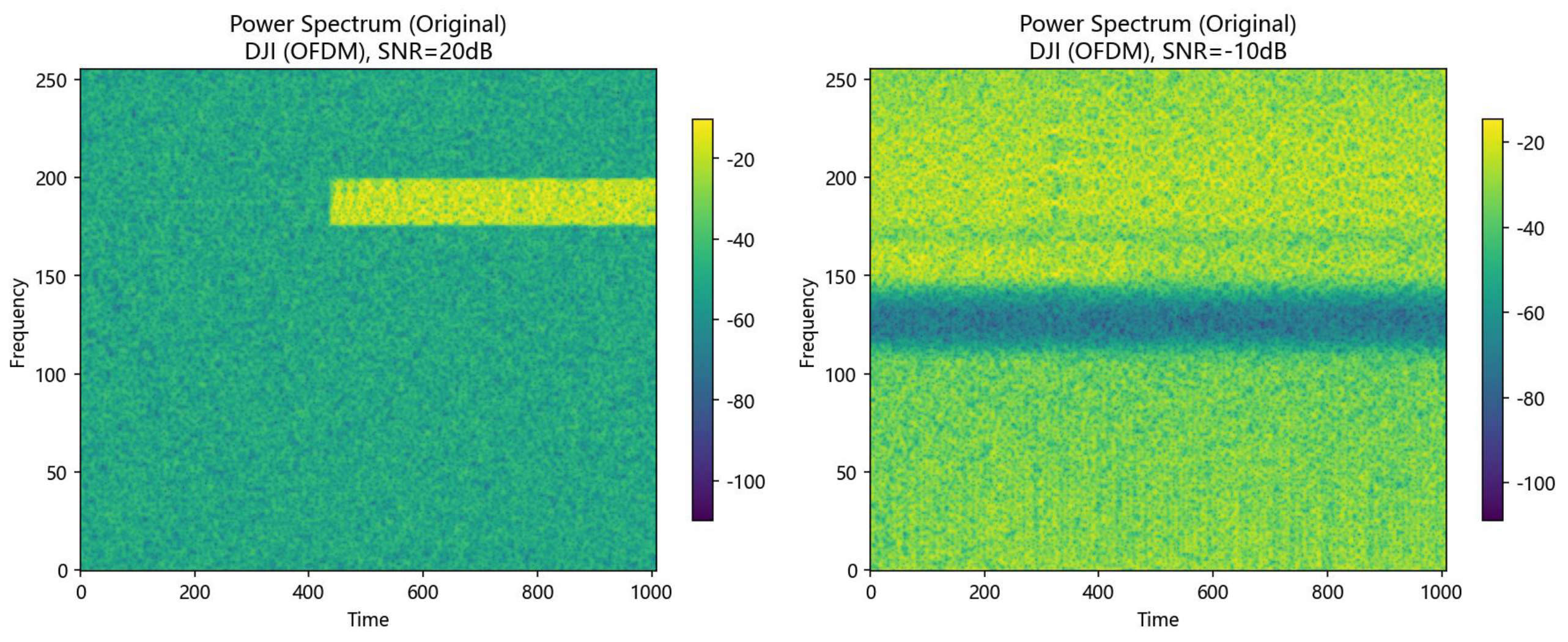
where $h\left[n\right]$ denotes the propagation channel response, and $v\left[n\right]$ denotes additive noise and interference. As reception distance increases, path loss reduces the received power, and noise increasingly obscures the effective signal structure. Low-SNR identification is therefore hindered by weaker energy, degraded local time-frequency textures, and blurred boundaries between similar models. It also becomes more difficult to exploit the structural priors of the signal. Figure 1 shows representative UAV RF spectrograms at SNRs of 20 dB and $-10$ dB.

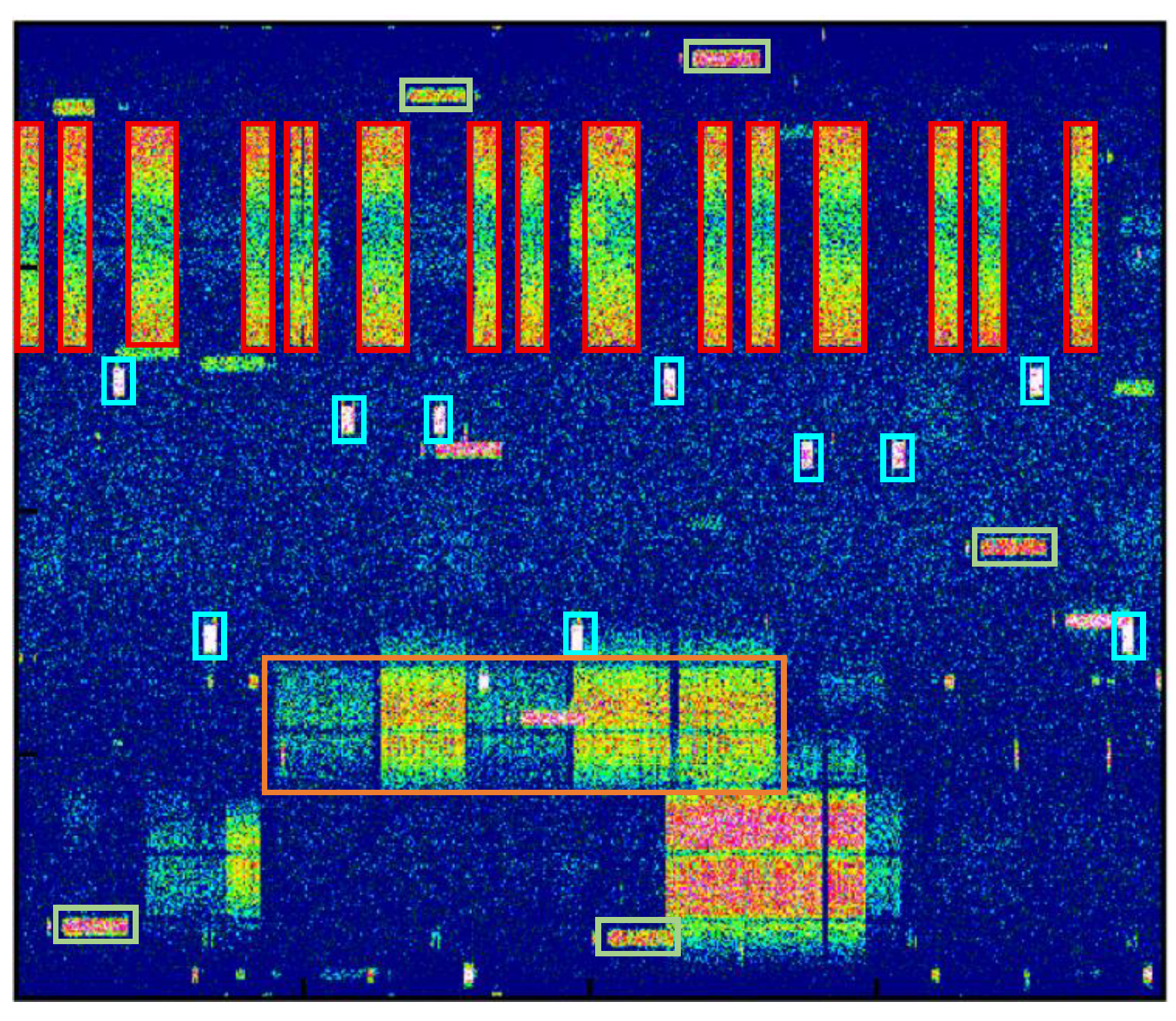
The quality of RSP statistics depends directly on the structural richness of the input multi-channel spectrogram. However, UAV RF signals contain communication components at different scales. Remote-control links often form stable narrowband structures that require high-frequency resolution. Video transmission and protocol interactions may instead form wider-band bursts that require high temporal resolution. Figure 2 illustrates these structures and relevant Wi-Fi and Bluetooth interference.

Although STFT can provide a two-dimensional time-frequency representation, its window length determines an inherent trade-off between time resolution and frequency resolution. As a result, a single time-frequency scale cannot satisfy the observation requirements of both types of signal structure. Under low SNR, this problem becomes more pronounced: a window that is too short weakens the frequency detail of stable narrowband components, whereas a window that is too long smooths short-time burst structures. We therefore adopt multi-resolution STFT to provide complementary multi-scale observations of weak time-frequency structures for both CNN feature learning and RSP geometric statistics.

Different STFT branches correspond to different time-frequency resolutions. A short window captures burst changes more sensitively but has lower frequency resolution, whereas a long window distinguishes stable frequency components more clearly but localizes transient variations less accurately. The choice of resolution is closely related to the physical form of the UAV RF signal.

3.2. Riemannian Structure Preservation

RSP is the core contribution of the proposed method. Existing deep models primarily learn local amplitude textures and underuse structural priors within RF signals. In multi-channel data, local channel correlations and second-order statistics reflect modulation, hardware, propagation, and receiver-position differences. These structures can be more stable than pointwise amplitudes under low SNR and long-range attenuation. RSP builds local SPD covariance structures and distills their geometric relationships into a training-stage relational teacher signal. This process improves embedding structure and discriminability without changing the inference path.

3.2.1. SPD Structure Prior of Multi-Channel RF Signals

In addition to amplitude texture, multi-channel RF spectrograms also encode local correlation structures. For a local time-frequency window, each time-frequency point within the window can be represented as a cross-channel vector ${\mathbf{x}}_{uv}\in {\mathbb{R}}^C$, where C is the number of spectrogram channels. Specifically, a $7\times 7$ local window $\mathcal{N}(f,t)$ is taken around position $(f,t)$, and its local channel covariance matrix is defined as

$$\mathsf{\Sigma }(f,t)={\displaystyle \frac{1}{M-1}}\sum _{(u,v)\in \mathcal{N}(f,t)}({\mathbf{x}}_{uv}-\overline{\mathbf{x}}){({\mathbf{x}}_{uv}-\overline{\mathbf{x}})}^{\top }+ϵ{\mathbf{I}}_C,$$

(3)

where M is the number of time-frequency points in the window, $\overline{\mathbf{x}}$ is the mean channel vector in the window, and ${\mathbf{I}}_C$ is the identity matrix. This $7\times 7$ neighborhood is defined independently on each STFT branch’s own discrete time-frequency grid. Because the three branches use different hop sizes and frequency-bin widths (Section 4.3), the same $7\times 7$ pixel window spans different physical time-frequency extents at each scale; for DroneRFa at $f_s=100$ MHz, the three branches cover approximately $35.8\mathsf{\mu }\mathrm{s}\times 684$ kHz, $71.7\mathsf{\mu }\mathrm{s}\times 342$ kHz, and $143.4\mathsf{\mu }\mathrm{s}\times 171$ kHz, respectively. The cross-scale ratio features in Equation (12) therefore compare statistics computed on scale-specific discrete pixel grids rather than on a single, physically co-registered time-frequency block, so we read them as relative, pipeline-consistent responses rather than measures of physical co-location across scales. The regularization term $ϵ{\mathbf{I}}_C$ ensures positive definiteness. For 2-channel input, $ϵ$ is set to ${10}^{-6}$; for inputs with more than two channels, $ϵ$ is set to ${10}^{-5}$. After adding the regularization term, the covariance matrix lies in the SPD matrix space:

$$\mathsf{\Sigma }(f,t)\in {\mathcal{S}}_{++}^C.$$

(4)

The local covariance matrix $\mathsf{\Sigma }(f,t)$ characterizes the channel correlation structure within a local region of the spectrogram. Compared with single-point energy values, this structure aggregates the statistical information of the local neighborhood and is more stable against random noise. For 4-channel dual-RF input, the SPD matrix can also represent the cross-channel correlation between the two receivers. It thus carries discriminative information conveyed by spatial reception differences, propagation-path differences, and hardware characteristics.

Each SPD covariance matrix is an element of the SPD manifold ${\mathcal{S}}_{++}^C$, whose geometry is non-Euclidean. Directly flattening an SPD matrix may discard its positive-definite structure and distort geometric distance relationships. To measure the local covariance structure stably, we adopt the Log-Euclidean representation, that is, we take the logarithm of the SPD matrix after eigendecomposition:

$$\log \left(\mathsf{\Sigma }\right)=\mathbf{U}\mathrm{diag}(\log {\lambda }_1,\dots ,\log {\lambda }_C){\mathbf{U}}^{\top },$$

(5)

where ${\lambda }_i$ and $\mathbf{U}$ are the eigenvalues and eigenvectors of the SPD matrix, respectively. In the log domain, the geometric difference between SPD matrices can be measured stably by the Frobenius norm. This property allows the local covariance structure to serve as a geometric statistical prior that constrains the sample relationships in the deep embedding space. In implementation, a $2\times 2$ analytical logarithm formula is used for $C=2$ to improve efficiency, while eigendecomposition is used for $C>2$.

3.2.2. Noise-Referenced Riemannian Geometric Statistical Maps

To measure geometric deviation from the noise background, we introduce a noise reference matrix. Before each fold, only training-set noise samples are used. For each STFT scale, we compute a Riemannian mean under the Log-Euclidean metric. Each SPD matrix is mapped through the matrix logarithm, averaged in Euclidean space, and mapped back through the matrix exponential. The resulting ${\mathsf{\Sigma }}_{\mathrm{ref}}$ is the geometric center of the noise covariance structure. The Riemannian distance at each position is defined as

$$d_{\mathrm{LE}}(f,t)={∥\log \left(\mathsf{\Sigma }(f,t)\right)-\log \left({\mathsf{\Sigma }}_{\mathrm{ref}}\right)∥}_F,$$

(6)

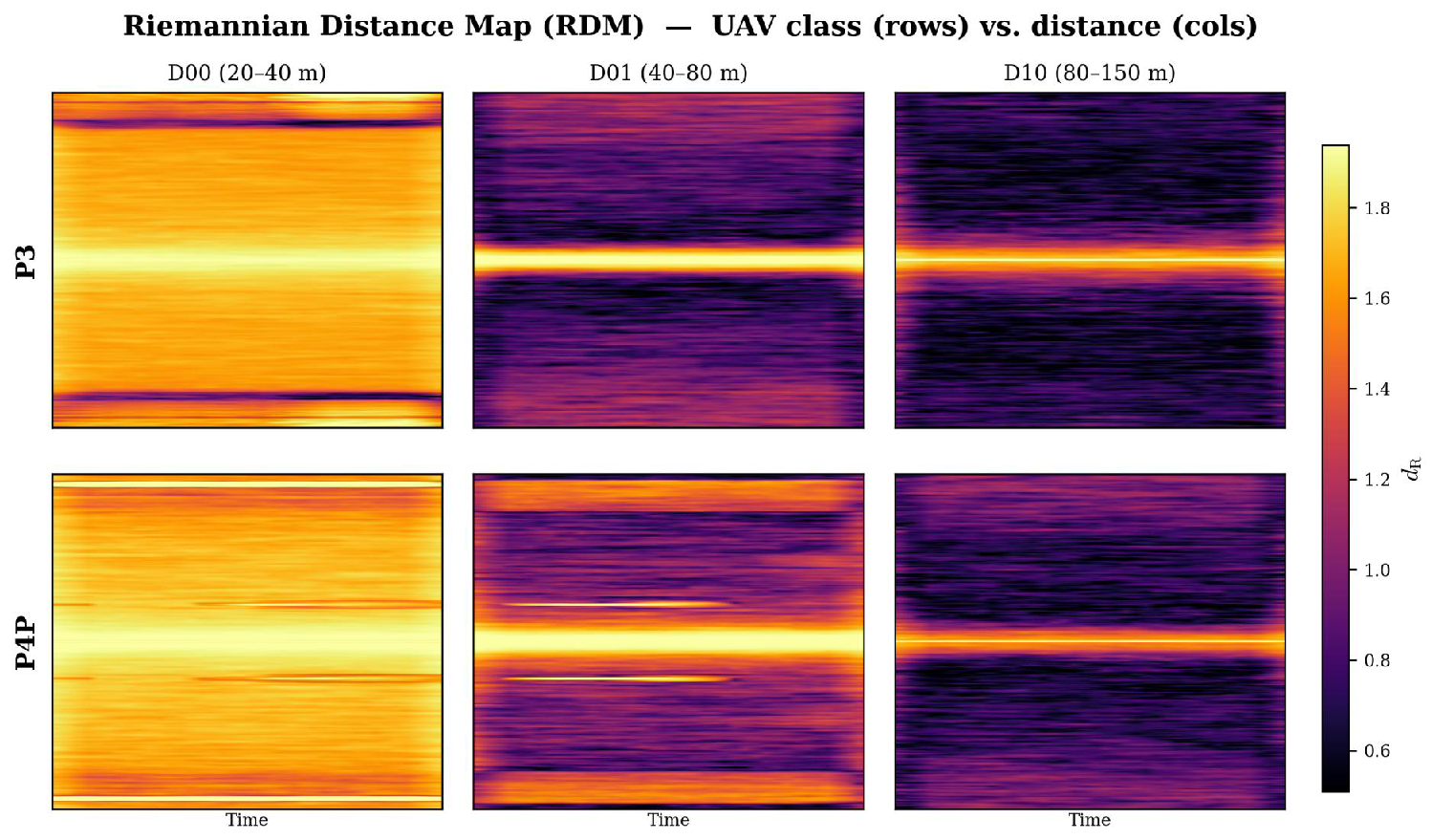
and, after logarithmic compression, the Riemannian distance map (RDM) is defined as

$$\mathrm{RDM}(f,t)=\log (1+d_{\mathrm{LE}}(f,t)).$$

(7)

The RDM reflects the degree of deviation of the local time-frequency structure relative to the noise background. Under low SNR, amplitude features may be corrupted by strong noise, but the local covariance structure may still preserve part of the signal correlation. The RDM therefore provides a complementary structural description that is robust to amplitude degradation.

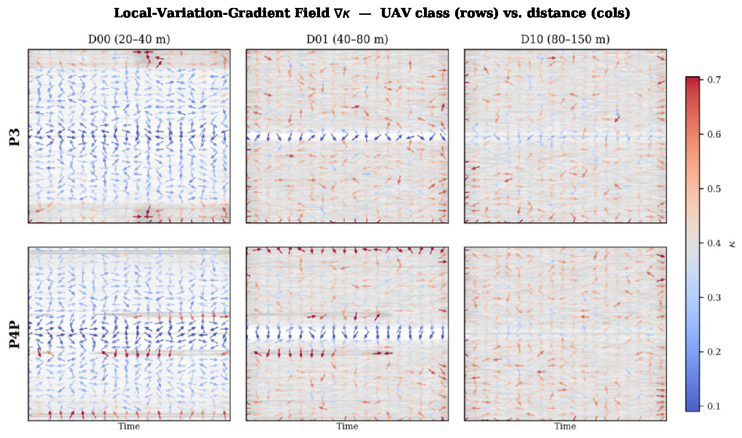
RSP focuses not only on the magnitude of local structural deviation from noise but also on the magnitude of covariance variation across the time-frequency plane. To this end, we take discrete differences of the log-domain SPD field along the frequency and time axes to approximate the local variation field, which we denote $\kappa$:

$$\kappa (f,t)=\log \left(1+{∥{\displaystyle \frac{\partial \log \mathsf{\Sigma }}{\partial f}}∥}_F+{∥{\displaystyle \frac{\partial \log \mathsf{\Sigma }}{\partial t}}∥}_F\right).$$

(8)

In essence, $\kappa (f,t)$ measures the local magnitude of geometric variation of the SPD structure on the time-frequency plane. For UAV RF signals, during frequency hops, modulation transitions, or transient onsets, the covariance structure of adjacent time-frequency positions changes sharply and $\kappa$ is large, whereas in stable continuous-wave regions $\kappa$ is small. We use the symbol $\kappa$ for convenience, but emphasize that it is a first-order finite-difference magnitude of the log-SPD field along frequency and time, not a Riemannian sectional, Gaussian, or other differential-geometric curvature.

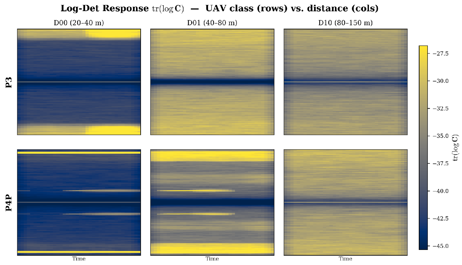
In addition, we compute the log-determinant response to characterize the volume or energy spread of the local covariance matrix:

$$G_m(f,t)=\log \det {\mathsf{\Sigma }}_m(f,t)=\mathrm{tr}\left(\log {\mathsf{\Sigma }}_m(f,t)\right).$$

(9)

The RDM, the local variation field, and the log-determinant response characterize the Riemannian geometric structure of the signal from three complementary perspectives, namely the geometric deviation relative to noise, the complexity of local structural variation, and the covariance volume information.

3.2.3. Multi-Scale Riemannian Statistical Vector

To limit computational complexity, RSP extracts compact statistics from the three structural maps. For sample i at scale m, ${\mathbf{D}}_{i,m}$, ${\mathbf{K}}_{i,m}$, and ${\mathbf{G}}_{i,m}$ denote the RDM, local variation, and log-determinant maps. Each scale yields 15 quantities. The RDM contributes its mean, standard deviation, maximum, median, skewness, kurtosis, spatial entropy, and high-response ratio ${\rho }_D$. The local variation field contributes its mean, standard deviation, maximum, and skewness. The remaining quantities are the RDM-local-variation correlation and the mean and standard deviation of the log-determinant response:

$$\begin{array}{c}{\mathbf{z}}_{i,m}=[{\mu }_D,{\sigma }_D,\max D,\mathrm{median}\left(D\right),\mathrm{skew}\left(D\right),\mathrm{kurt}\left(D\right),H\left(D\right),{\rho }_D,\\ {\mu }_{\kappa },{\sigma }_{\kappa },\max \kappa ,\mathrm{skew}\left(\kappa \right),{\rho }_{D\kappa },{\mu }_G,{\sigma }_G].\end{array}$$

(10)

These statistics compress the complete spectrogram into a low-dimensional representation while retaining structural magnitude, dispersion, extrema, distribution shape, spatial complexity, and covariance-volume information. The statistics of the three STFT scales are concatenated as

$${\mathbf{z}}_i=[{\mathbf{z}}_{i,1};{\mathbf{z}}_{i,2};{\mathbf{z}}_{i,3}]\in {\mathbb{R}}^{45}.$$

(11)

To further characterize the variation of the structural response of the same sample across different STFT scales, we construct six cross-scale ratio features composed of the ratios of the RDM mean and the local-variation mean between adjacent scales and across scales:

$${\mathbf{q}}_i=\left[{\displaystyle \frac{{\mu }_D^{\left(2\right)}}{{\mu }_D^{\left(1\right)}+{\epsilon }_q}},{\displaystyle \frac{{\mu }_D^{\left(3\right)}}{{\mu }_D^{\left(2\right)}+{\epsilon }_q}},{\displaystyle \frac{{\mu }_D^{\left(3\right)}}{{\mu }_D^{\left(1\right)}+{\epsilon }_q}},{\displaystyle \frac{{\mu }_{\kappa }^{\left(2\right)}}{{\mu }_{\kappa }^{\left(1\right)}+{\epsilon }_q}},{\displaystyle \frac{{\mu }_{\kappa }^{\left(3\right)}}{{\mu }_{\kappa }^{\left(2\right)}+{\epsilon }_q}},{\displaystyle \frac{{\mu }_{\kappa }^{\left(3\right)}}{{\mu }_{\kappa }^{\left(1\right)}+{\epsilon }_q}}\right]\in {\mathbb{R}}^6,$$

(12)

where ${\epsilon }_q$ is a constant that prevents division by zero. This feature reflects whether the signal structure is dominated by short-time bursts or stable narrowband continuity and provides cross-scale relative geometric information. The final 51-dimensional Riemannian statistical vector of the i-th sample is obtained as

$${\mathbf{r}}_i=[{\mathbf{z}}_i;{\mathbf{q}}_i]\in {\mathbb{R}}^{51}.$$

(13)

The 45 statistics in ${\mathbf{z}}_i$ and the 6 ratios in ${\mathbf{q}}_i$ are concatenated without per-dimension standardization before the Euclidean distance in Equation (14) is computed; only non-finite values are replaced, and the scale difference across dimensions is absorbed by the median-heuristic kernel bandwidth $\sigma$ rather than by dimension-wise rescaling. The corresponding min–max normalized “normalized mean profile,” visualized later in this section, is used only for qualitative visualization and plays no role in training. A batch-wise per-dimension z-score variant of ${\mathbf{r}}_i$, evaluated on MRS-Net-4ch under session-level grouped cross-validation (Section 5.1.3), gives no consistent accuracy gain over this unstandardized vector (Supplementary Materials), which motivates the simpler design retained here.

After obtaining ${\mathbf{r}}_i$, RSP does not use this vector as an explicit classification feature at inference; instead, it uses ${\mathbf{r}}_i$ to define the structural relationship between samples. Specifically, ${\mathbf{r}}_i$ lies in a 51-dimensional statistical feature space derived from the RDM, local variation field, log-determinant response, and cross-scale ratio features. The smaller the distance between two samples in this space, the more similar they are in terms of the local SPD covariance structure, the geometric deviation relative to noise, and the cross-scale response pattern.

To convert this high-dimensional spatial distance into a continuous and stable structural similarity, we define the RSP structural metric using a Gaussian kernel function:

$$K_R(i,j)=\exp \left(-{\displaystyle \frac{\parallel {\mathbf{r}}_i-{\mathbf{r}}_j{\parallel }_2^2}{2{\sigma }^2}}\right),$$

(14)

where $\parallel {\mathbf{r}}_i-{\mathbf{r}}_j{\parallel }_2^2$ denotes the high-dimensional distance between two samples in the 51-dimensional Riemannian statistical space, and the kernel bandwidth $\sigma$ is determined adaptively by the median of the pairwise distances. This Gaussian similarity is essentially a kernelized metric based on the high-dimensional distance: when the Riemannian statistical structures of two samples are close, $K_R$ approaches 1; when their structures differ substantially, $K_R$ decays rapidly. In this way, RSP converts the Riemannian statistical description of a single sample into a structural relation matrix among the samples within a batch. This matrix provides a structural teacher signal for the subsequent relational alignment in the CNN embedding space.

3.2.4. Effectiveness Analysis of the Riemannian Statistics

Whether the Riemannian statistical vector defined above can provide an effective prior for classification depends on whether different types of signals exhibit distinguishable structural characteristics in this statistical space. To examine class separability and distance robustness qualitatively, we visualize three two-dimensional response maps for different UAV classes under different distance conditions.

In these visualizations, the RDM is represented as a continuous heat map showing the deviation of the local covariance from the noise-reference SPD centroid. The local variation field is represented by overlaying gradient arrows on the variation-response background, which highlights the direction of variation and the textural characteristics of the local geometric structure. The log-determinant response is represented as a block-wise heat map showing the volume or energy spread of the local covariance. As shown in Figure 3, Figure 4 and Figure 5, two representative UAV signal classes present clearly different structures in the Riemannian distance, local variation, and log-determinant response maps.

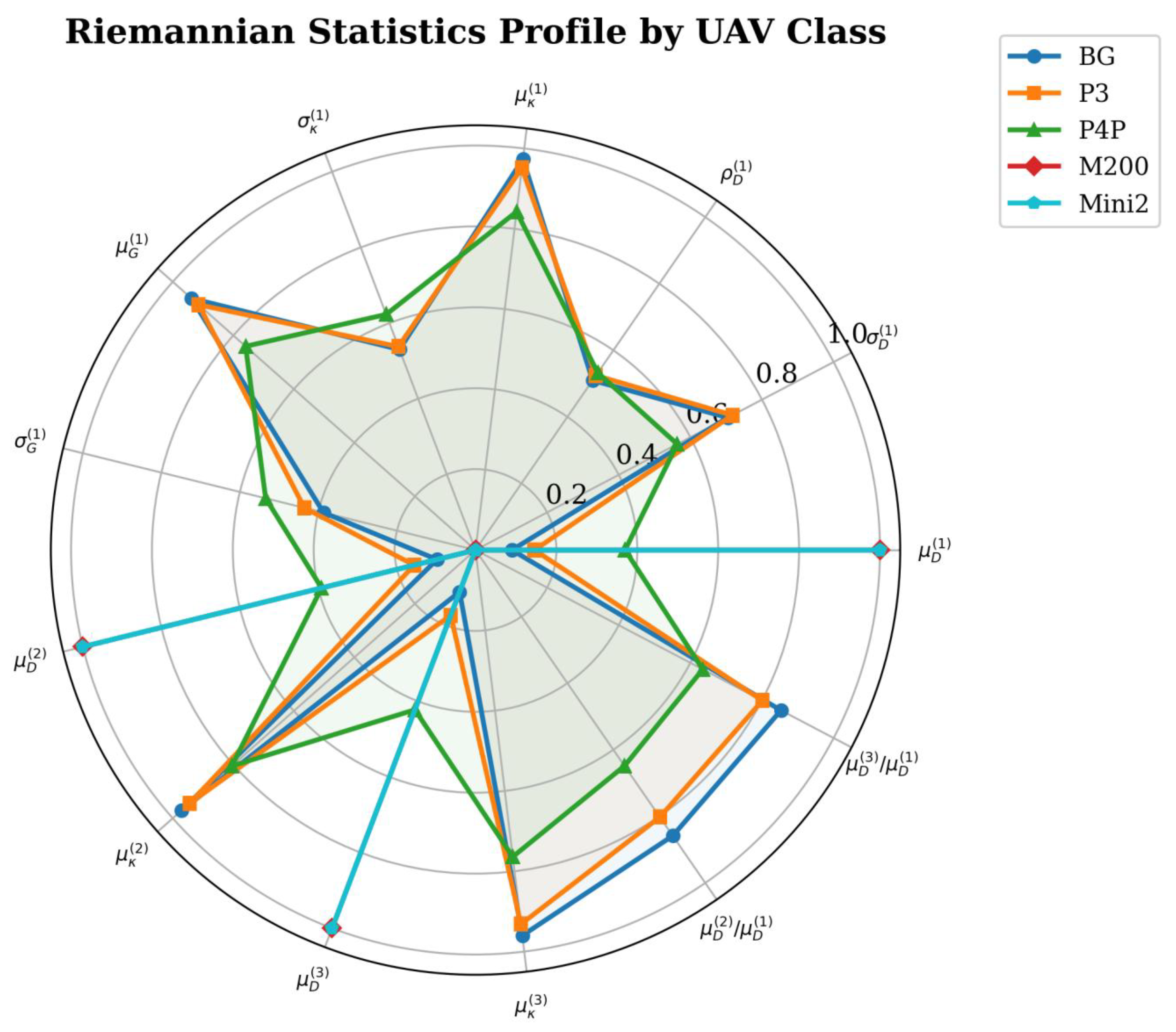
Figure 6 shows the normalized mean profile of five representative classes (Background, DJI Phantom 3, DJI Phantom 4 Pro, DJI Matrice 200, and DJI Mini 2) across 13 key Riemannian statistical dimensions.

Different signal types show systematic differences along statistical dimensions such as the RDM mean ${\mu }_D$, the local-variation mean ${\mu }_{\kappa }$, the log-determinant response ${\mu }_G$, and the cross-scale ratio ${\mu }_D^{\left(3\right)}/{\mu }_D^{\left(1\right)}$. For example, the cross-scale RDM ratio of the DJI Mini 2 is markedly higher than that of the other models, whereas Background has a distinctive profile shape along the variation-related dimensions. These differences originate from the intrinsic differences among UAV models in modulation scheme, frequency usage, and hardware characteristics. Different modulation schemes produce different local covariance structures on the time-frequency plane, while different transmission links and antenna characteristics are encoded as differentiated geometric information in the SPD matrix through cross-channel covariance.

The visualizations show that different UAV classes exhibit distinct structures in the two-dimensional response maps, including variations in response-band location, intensity distribution, and local variation texture. These qualitative results suggest that the statistics capture differences among UAV signals and exhibit promising class separability. The same class also maintains a similar dominant response pattern across distance conditions, suggesting that these statistics are relatively stable under distance variation.

Therefore, the Riemannian statistics strengthen the differences among UAV signals and provide a useful feature basis for UAV identification under distance-induced attenuation.

3.3. Loss Design

To ensure both classification accuracy and structure preservation, our loss function consists of two parts: a CosFace hyperspherical discriminative loss that enhances class separability and an RSP loss that preserves second-order Riemannian statistical relationships. The two jointly act on the CNN embedding space, making it both class-discriminative and able to preserve the second-order relationships inherent in the multi-channel RF signal.

3.3.1. Hyperspherical Discriminative Embedding

To endow the RSP-constrained embedding space with strong class separability, we introduce the CosFace hyperspherical metric into embedding learning. The conventional cross-entropy loss can optimize classification correctness but does not explicitly constrain intra-class compactness or the inter-class geometric margin. Under low SNR, samples of the same class may be dispersed by noise perturbation, while different UAV models may overlap in the embedding space because of similar communication protocols, frequency bands, or modulation schemes. This can lead to unstable classification boundaries for similar models.

Given the multi-resolution spectrogram S, the feature extractor of the m-th branch is denoted by $g_m(·)$, and its output after pooling is

$${\mathbf{f}}_m=g_m\left(S_m\right),m=1, \dots , M.$$

(15)

The features of all branches are concatenated as

$${\mathbf{f}}_{\mathrm{cat}}=[{\mathbf{f}}_1; {\mathbf{f}}_2; \dots ; {\mathbf{f}}_M].$$

(16)

The fusion layer maps the multi-resolution features into a unified embedding:

$$\mathbf{e}={\mathbf{W}}_f\phi \left({\mathbf{f}}_{\mathrm{cat}}\right)+{\mathbf{b}}_f,\mathbf{e}\in {\mathbb{R}}^d,$$

(17)

where $\phi (·)$ denotes a nonlinear transformation implemented with ReLU and dropout, and ${\mathbf{W}}_f$ and ${\mathbf{b}}_f$ are the parameters of the fusion layer. This embedding receives both the class supervision of CosFace and the structural supervision of RSP.

CosFace first applies L2 normalization to the embedding vector and the classification weights:

$${\widehat{\mathbf{e}}}_i={\displaystyle \frac{{\mathbf{e}}_i}{\parallel {\mathbf{e}}_i{\parallel }_2}},{\widehat{\mathbf{w}}}_k={\displaystyle \frac{{\mathbf{w}}_k}{\parallel {\mathbf{w}}_k{\parallel }_2}}.$$

(18)

The cosine similarity between the i-th sample and class k is defined as

$$\cos {\theta }_{k,i}={\widehat{\mathbf{e}}}_i^{\top }{\widehat{\mathbf{w}}}_k.$$

(19)

An additive cosine margin m is imposed on the target class $y_i$, and a scaling factor s adjusts the logit range. The loss is

$${\mathcal{L}}_{\mathrm{CF}}=-{\displaystyle \frac{1}{N}}{\displaystyle \sum _{i=1}^N}\log {\displaystyle \frac{\exp \left(s(\cos {\theta }_{y_i}-m)\right)}{\exp \left(s(\cos {\theta }_{y_i}-m)\right)+{\sum }_{k\ne y_i}\exp \left(s\cos {\theta }_k\right)}},$$

(20)

where N is the batch size, and the margin m and the scaling factor s are initialized according to the data conditions. This loss makes samples of the same class more compact on the hypersphere and forms a larger angular margin between different classes. It thereby mitigates the blurring of class boundaries between UAV models under low SNR and provides a discriminative embedding space for the structural constraint of RSP.

3.3.2. Pairwise Similarity Alignment and the RSP Loss

Because the two spaces differ in both dimension and semantics, the key to RSP is not to force the CNN feature vector of each sample to equal its Riemannian statistical vector, but to align the similarity relationships between samples. For a mini-batch of N samples, pairwise similarity matrices are constructed in the statistical feature space and in the CNN embedding space, respectively.

In the Riemannian statistical space, the Gaussian kernel similarity is computed from the Riemannian statistical vectors based on Equation (14). This similarity can be understood as a structural metric based on high-dimensional distance, describing how close the local SPD statistical structures of two samples are. In the CNN embedding space, the similarity between samples is defined as the cosine similarity, so as to stay consistent with the angular discriminative space of CosFace:

$$K_E(i,j)={\displaystyle \frac{{\mathbf{e}}_i·{\mathbf{e}}_j}{{\parallel {\mathbf{e}}_i\parallel }_2{\parallel {\mathbf{e}}_j\parallel }_2}}.$$

(21)

The two similarity matrices are then row-wise normalized by softmax, which converts the similarity between each sample and the others into a relative distribution. This normalization focuses on the ranking relation of “which samples are more similar to sample i” and eliminates the influence of the inconsistent numerical ranges of the two matrices. The RSP loss is finally defined as the Frobenius distance between the normalized similarity matrices:

$${\mathcal{L}}_{\mathrm{RSP}}={\displaystyle \frac{1}{N^2}}{∥\mathrm{softmax}\left(K_R\right)-\mathrm{softmax}\left(K_E\right)∥}_F^2.$$

(22)

This loss makes the CNN embedding space preserve the pairwise relationships in the Riemannian statistical space. If two samples are similar in their SPD-manifold statistical structure, their CNN embeddings should also maintain high similarity; conversely, if two samples have very different local covariance structures, their embedding representations should be pushed apart.

The RF signals of different UAV models differ in modulation scheme, frequency usage, and hardware characteristics. These differences are encoded in the SPD matrices as local covariance structures rather than only as spectral amplitude patterns, and the resulting SPD similarity relations are more robust to random amplitude noise than pointwise amplitude features. Distilling them into the CNN embedding space therefore provides an additional class-discriminative prior under low SNR.

3.3.3. Overall Loss Function

The overall training objective is the sum of the CosFace classification loss and the RSP structure-preserving loss:

$${\mathcal{L}}_{\mathrm{total}}={\mathcal{L}}_{\mathrm{CF}}+\alpha \left(t\right){\mathcal{L}}_{\mathrm{RSP}},$$

(23)

where $\alpha \left(t\right)$ is the RSP loss weight. Because the deep embedding has not yet formed a stable class structure in the early training stage, imposing a strong geometric constraint too early may affect the learning of the classification boundary. Therefore, a linear warm-up strategy is adopted to gradually increase the RSP weight:

$$\alpha \left(t\right)={\alpha }_{\max }\min \left({\displaystyle \frac{t}{T_w}},1\right),$$

(24)

where t denotes the current epoch, $T_w$ denotes the number of warm-up epochs, and ${\alpha }_{\max }$ denotes the maximum weight.

4. MRS-Net Network Framework

4.1. Overall Framework of MRS-Net

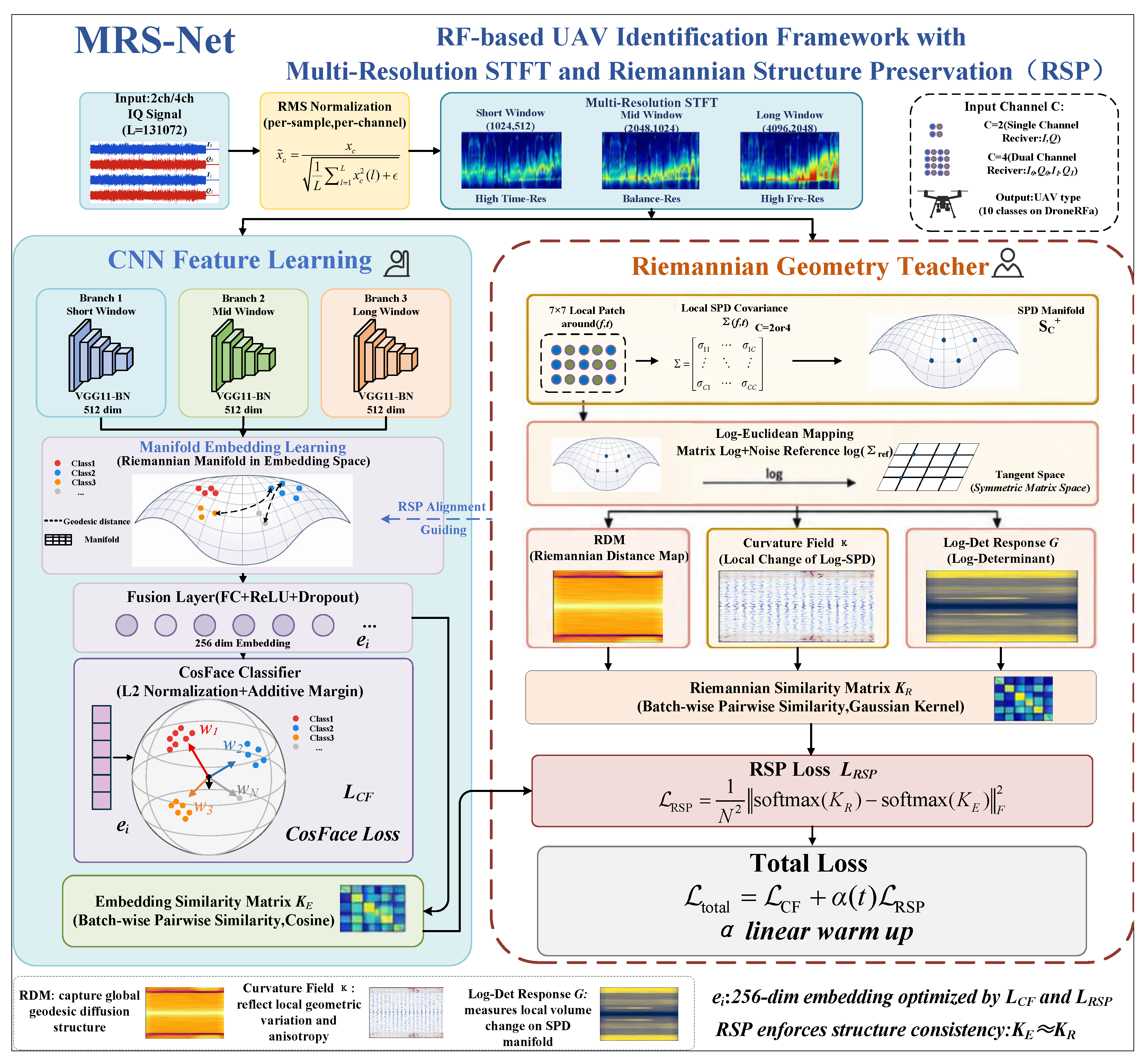
Based on the RSP method described above, we build MRS-Net for low-SNR drone RF identification. At its core, RSP injects stable local SPD Riemannian statistics from multi-channel RF signals into deep feature learning as a training-stage teacher signal. Multi-resolution STFT improves the capture of weak time-frequency structures and provides RSP with richer covariance information. CosFace improves inter-class separability in the embedding space, whereas the Gaussian kernel defines pairwise structural similarity for RSP. These components address three key bottlenecks in low-SNR RF identification: structural-prior utilization, weak-signal observation, and embedding discrimination.

Figure 7 summarizes the forward pipeline of MRS-Net. Each raw I/Q segment first undergoes root mean square (RMS) normalization per sample and channel. Multi-resolution STFT then converts the segment into multi-channel time-frequency representations spanning complementary time and frequency scales. Parallel CNN branches extract multi-scale features and fuse them into a unified embedding, while the CosFace head performs classification in the normalized embedding space. During training, the RSP branch constructs SPD covariance structures from the same batch of multi-channel spectrograms. It extracts the noise-referenced RDM, local variation field, log-determinant response, and multi-scale Riemannian statistical vectors. Pairwise similarity alignment then transfers these second-order geometric relationships into the CNN embedding space.

During training, ${\mathbf{r}}_i$ serves as a fixed teacher representation derived from local SPD statistics, and its gradient is detached during backpropagation. Gradients update the network parameters only through the CNN embedding ${\mathbf{e}}_i$. This design establishes a one-way teacher–student relationship and avoids numerical instability along the matrix-logarithm backpropagation path. Because the RSP branch is removed at inference, it adds no SPD computation to online operation.

4.2. Input Representation and Preprocessing

We consider two input forms. The 2-channel input represents the I/Q components of a single RF receiver,

$${\mathbf{x}}_{2\mathrm{c}\mathrm{h}}=[{\mathbf{I}}_0,{\mathbf{Q}}_0]\in {\mathbb{R}}^{2\times L},$$

(25)

and the 4-channel input concatenates the I/Q components of two RF receivers,

$${\mathbf{x}}_{4\mathrm{c}\mathrm{h}}=[{\mathbf{I}}_0,{\mathbf{Q}}_0,{\mathbf{I}}_1,{\mathbf{Q}}_1]\in {\mathbb{R}}^{4\times L},$$

(26)

where subscripts 0 and 1 index the two receivers. The 2-channel input contains only the I/Q relationship within one receiver, whereas the 4-channel input also captures correlations across receivers. In DroneRFa, the two receivers’ I/Q sequences are stored in the same recording file and sliced using identical start and end sample indices on a shared sampling clock; we treat them as synchronously acquired and do not apply any additional cross-receiver time-delay estimation or resampling before forming Equation (26) or the covariance in Equation (3). Any residual hardware-level timing offset between the two receivers is therefore absorbed into the off-diagonal cross-receiver terms of the SPD matrix rather than corrected explicitly. The goal is to learn the classification function

$$\widehat{y}=F_{\theta }\left(\mathbf{x}\right),$$

(27)

where $\mathbf{x}$ is the input I/Q segment, $\widehat{y}$ is the predicted class, and $F_{\theta }$ denotes the complete model. It comprises the multi-resolution time-frequency representation, CNN encoder, CosFace classification head, and RSP training constraint.

To eliminate the amplitude-scale differences between acquisition segments caused by received power and distance attenuation, RMS normalization is applied to each channel of each sample:

$${\tilde{x}}^{\left(c\right)}\left[l\right]={\displaystyle \frac{x^{\left(c\right)}\left[l\right]}{\sqrt{\frac{1}{L}{\sum }_{l=0}^{L-1}{\left|x^{\left(c\right)}\left[l\right]\right|}^2+ϵ}}},$$

(28)

where c indexes the channel, and $ϵ$ is a stability constant that prevents division by zero. This normalization encourages the model to rely on relative time-frequency structure rather than absolute power, thereby mitigating amplitude shifts caused by distance-dependent attenuation.

4.3. Multi-Resolution Time-Frequency Representation

The geometric, statistical quality of RSP depends directly on the structural richness of the input multi-channel spectrogram. STFT converts the normalized complex signal into a spectrogram, with the m-th branch defined as

$$S_m(f,t)={\displaystyle \sum _{n=0}^{N_{\mathrm{fft},m}-1}}s[t{H}_m+n]w\left[n\right]\exp \left(-j{\displaystyle \frac{2\pi fn}{N_{\mathrm{fft},m}}}\right),$$

(29)

where $N_{\mathrm{fft},m}$ is the window length or FFT size, $H_m$ is the hop size, and $w\left[n\right]$ is the window function. We set $H_m=N_{\mathrm{fft},m}/2$ for each branch, yielding approximately 50% overlap and limiting the loss of temporal information.

We use short-, medium-, and long-window STFT branches to construct the multi-resolution input. Their window-length and hop-size settings are $(1024,512)$, $(2048,1024)$, and $(4096,2048)$, respectively. The short-window branch captures burst changes, the medium-window branch provides a compromise, and the long-window branch preserves stable frequency components. These settings correspond to the multi-scale time-frequency morphology of UAV RF signals discussed in Section 3.1.

For single-RF (2-channel I/Q) input, the real and imaginary parts of the STFT complex spectrum form a two-channel spectrogram:

$$S_m=[\mathrm{Re}\left(S_m\right),\mathrm{Im}\left(S_m\right)].$$

(30)

For dual-RF (4-channel I/Q) input, the two complex spectra are computed separately and concatenated along the channel dimension:

$$S_m=[\mathrm{Re}\left(S_{m,0}\right),\mathrm{Im}\left(S_{m,0}\right),\mathrm{Re}\left(S_{m,1}\right),\mathrm{Im}\left(S_{m,1}\right)].$$

(31)

The multi-resolution representation provides the CNN with amplitude- and phase-related information at multiple scales while supplying RSP with richer local covariance structures. In the 4-channel case, concatenating spectra across receivers increases both the dimension and geometric information capacity of the local SPD matrix. This richer representation provides a stronger second-order statistical basis for Riemannian Structure Preservation.

4.4. CNN Feature Extraction, Fusion, and Inference

MRS-Net uses parallel CNN branches to process spectrograms at different STFT scales. Each branch uses VGG11-BN to extract local texture, frequency structure, and transient variations from its corresponding spectrogram. Each branch produces a 512-dimensional feature vector. The three features are concatenated into a 1536-dimensional representation and mapped by the fusion layer to a 256-dimensional embedding, following Equations (15)–(17).

The CosFace head uses this embedding for class discrimination in a normalized hyperspherical space. During training, RSP also aligns the embedding with a Riemannian statistical similarity matrix. The RSP branch extracts local SPD covariance matrices from the multi-channel spectrogram and applies Log-Euclidean mapping. It then derives the RDM, local variation field, log-determinant response, and a 51-dimensional multi-scale Riemannian statistical vector. This vector defines a structural similarity matrix, which is aligned with the cosine similarity matrix of the CNN embeddings.

During training, pairwise similarity alignment updates the CNN encoder and embedding layer to preserve sample relationships induced by the local SPD structure. At inference, the signal passes only through the trained feature-extraction and classification network. The resulting embedding retains the learned structural prior without requiring online Riemannian computation.

5. Experimental Evaluation and Results

This section evaluates MRS-Net under real propagation attenuation and controlled additive noise, focusing on whether RSP can exploit multi-channel local covariance priors. DroneRFa [27] combines outdoor propagation attenuation, distance variation, and dual-receiver multi-channel RF signals, making it the primary dataset for testing the RSP hypothesis. Noisy Drone RF [28] provides explicit SNR labels and supports complementary validation and cross-method comparison under additive noise. Progressive, parameter-aligned, and backbone ablations further isolate the contribution of each module and characterize the applicability boundary of RSP.

5.1. Datasets and Experimental Protocol

5.1.1. Datasets

We use two public datasets, Noisy Drone RF and DroneRFa, which represent complementary forms of low-SNR degradation. Noisy Drone RF uses additive white Gaussian noise (AWGN) to construct specific SNR levels and supports evaluation under controlled noise degradation. DroneRFa was collected outdoors using two RF receivers and characterizes signal-quality degradation by distance, more closely reflecting practical low-altitude monitoring.

Table 1. Summary of the datasets and evaluation roles.

Dataset	Classes	Sampling Rate	Input Form	Low-SNR Setting/Role
Noisy Drone RF	7	14 MHz	Single-RF complex I/Q	AWGN-defined SNR; controlled-noise evaluation
DroneRFa	10	100 MHz	Single-RF 2ch or dual-RF 4ch I/Q	Distance gradient; propagation and multi-channel evaluation

summarizes the main attributes of both datasets.

For DroneRFa, we select nine DJI drone classes and one background-noise class. The distance ranges are D00 (20–40 m), D01 (40–80 m), and D10 (80–150 m). Each sample is cropped to 131,072 points during training. The 2ch setting contains the I/Q components of one receiver, whereas the 4ch setting concatenates those of two receivers.

5.1.2. Model Variants and Implementation Details

To clarify the progression from a conventional CNN to RSP-guided learning, we construct the three model variants shown in

Table 2. Model variants used in the experiments. × and ✓ indicate whether the RSP structural teacher is used during training.

Method	STFT	Classification Loss	RSP Teacher	Description
SR-CNN	Single resolution	Cross-entropy	×	Single-resolution baseline
MR-Spherical	Multi-resolution	CosFace	×	Multi-resolution representation with CosFace
MRS-Net	Multi-resolution	CosFace + RSP	✓	Complete framework with RSP

.

On DroneRFa, SR-CNN uses $N_{\mathrm{fft}}=2048$ and $H=1024$. MR-Spherical and MRS-Net use $(1024,512)$, $(2048,1024)$, and $(4096,2048)$ for their three STFT branches. At a sampling rate of 100 MHz, these branches emphasize high temporal resolution, an intermediate time-frequency resolution, and high frequency resolution, respectively. For the shorter Noisy Drone RF signals, the STFT parameters are scaled according to the same multi-resolution principle.

Table 3. Training hyperparameters. N/A denotes hyperparameters that do not apply because RSP is not used on Noisy Drone RF (Table 2).

Parameter	Noisy Drone RF	DroneRFa
Optimizer	Adam	Adam
Initial learning rate	$5\times {10}^{-3}$	$2\times {10}^{-4}$
Weight decay	0	$5\times {10}^{-5}$
Batch size	8	16
Maximum epochs	50	60
Learning rate scheduler	ReduceLROnPlateau	ReduceLROnPlateau
Scheduler patience/factor	10/0.5	5/0.5
Gradient clipping	5.0	5.0
CosFace $s/m$	8.0/0.2	8.0/0.2
RSP ${\alpha }_{\max }$/warm-up epochs	N/A	0.1/10
RSP bandwidth $\sigma$	N/A	Auto (median heuristic)
Class balancing	WeightedRandomSampler	WeightedRandomSampler

lists the main training hyperparameters. All experiments use PyTorch 2.5.1 (CUDA 12.1) and torchaudio 2.5.1 and run on an NVIDIA RTX 4090 GPU with 24 GB of memory.

5.1.3. Evaluation Metric and Cross-Validation Protocol

Given the imbalanced class distribution in RF identification, we use balanced accuracy (BAcc) as the primary evaluation metric:

$$\mathrm{BAcc}={\displaystyle \frac{1}{K}}{\displaystyle \sum _{k=1}^K}{\displaystyle \frac{{\mathrm{TP}}_k}{{\mathrm{TP}}_k+{\mathrm{FN}}_k}},$$

(32)

where K is the number of classes, and ${\mathrm{TP}}_k$ and ${\mathrm{FN}}_k$ denote true positives and false negatives for class k, respectively. BAcc equals the macro-average of per-class recall and prevents majority classes from dominating the evaluation. All main experiments use 5-fold stratified cross-validation and report the mean ± standard deviation. For DroneRFa, joint class-and-distance labels guide stratification to balance both distributions across folds.

Each DroneRFa recording session is cut into multiple fixed-length slices (Section 4.4), and this protocol stratifies at the slice level without grouping by source session. Slices from the same session can therefore appear on both sides of a fold, so Table 4 and the associated ablations evaluate discrimination under matched acquisition conditions (in-session discrimination) rather than generalization to unseen recording sessions. As a stricter check, we additionally run session-level grouped 5-fold cross-validation, in which no slice from a given session appears on both sides of a fold; this changes what is being measured and yields lower absolute BAcc, so we report it as a separate cross-session check in Section 5.6 and the Supplementary Materials rather than substituting it into Table 4.

We report the cross-fold standard deviation as an indicator of training reproducibility under multi-channel low-SNR conditions. Because the five folds partition one fixed dataset rather than constituting independent draws, paired comparisons across folds are treated as descriptive rather than confirmatory. The corresponding p-values, 95% confidence intervals, and effect sizes appear in the Supplementary Materials and are not used in the main text to characterize the significance of a comparison.

5.2. Recognition Performance on DroneRFa

DroneRFa is the primary dataset used to evaluate the core RSP mechanism. Unlike the synthetic additive noise in Noisy Drone RF, it combines outdoor propagation attenuation, distance variation, and dual-receiver information. This combination tests whether MRS-Net can exploit cross-channel local covariance structures under degraded signal quality. Table 4 reports overall and distance-wise BAcc, together with the performance decrease from D00 to D10, for all six settings.

Table 4. Main results on DroneRFa under the slice-level, in-session 5-fold protocol of Section 5.1.3. A complementary session-level grouped cross-validation check is reported in Section 5.6 and the Supplementary Materials.

Input	Method	D00	D01	D10	Overall	D00–D10
2ch	SR-CNN	84.13 ± 3.14	69.90 ± 6.20	65.50 ± 4.07	77.02 ± 3.78	$-18.63$
2ch	MR-Spherical	90.70 ± 0.93	75.43 ± 2.28	74.10 ± 1.89	84.74 ± 0.94	$-16.60$
2ch	MRS-Net	88.97 ± 1.44	79.20 ± 1.44	75.00 ± 2.46	84.50 ± 1.48	$-13.97$
4ch	SR-CNN	79.33 ± 7.60	65.27 ± 10.36	61.30 ± 11.80	74.01 ± 12.11	$-18.03$
4ch	MR-Spherical	87.47 ± 11.69	73.37 ± 16.27	69.97 ± 16.96	83.20 ± 16.78	$-17.50$
4ch	MRS-Net	93.90 ± 1.72	79.63 ± 2.44	78.30 ± 1.10	90.30 ± 1.46	$-15.60$

Table 4. Main results on DroneRFa under the slice-level, in-session 5-fold protocol of Section 5.1.3. A complementary session-level grouped cross-validation check is reported in Section 5.6 and the Supplementary Materials.

Input	Method	D00	D01	D10	Overall	D00–D10
2ch	SR-CNN	84.13 ± 3.14	69.90 ± 6.20	65.50 ± 4.07	77.02 ± 3.78	$-18.63$
2ch	MR-Spherical	90.70 ± 0.93	75.43 ± 2.28	74.10 ± 1.89	84.74 ± 0.94	$-16.60$
2ch	MRS-Net	88.97 ± 1.44	79.20 ± 1.44	75.00 ± 2.46	84.50 ± 1.48	$-13.97$
4ch	SR-CNN	79.33 ± 7.60	65.27 ± 10.36	61.30 ± 11.80	74.01 ± 12.11	$-18.03$
4ch	MR-Spherical	87.47 ± 11.69	73.37 ± 16.27	69.97 ± 16.96	83.20 ± 16.78	$-17.50$
4ch	MRS-Net	93.90 ± 1.72	79.63 ± 2.44	78.30 ± 1.10	90.30 ± 1.46	$-15.60$

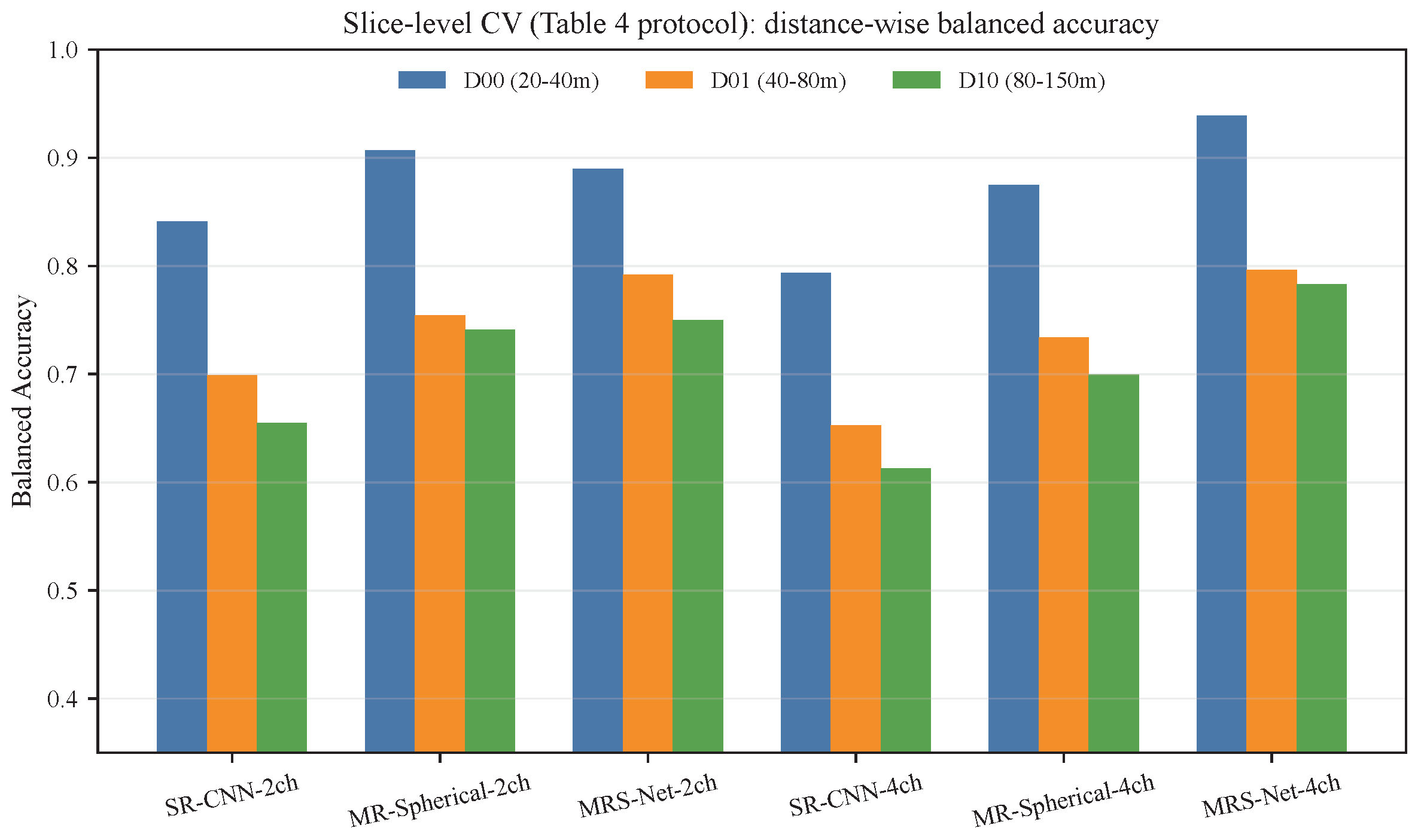
Figure 8 shows distance-wise BAcc on DroneRFa. Among the tested configurations, MRS-Net-4ch achieves the highest overall BAcc at 90.30%, exceeding SR-CNN-4ch by 16.29 percentage points (pp) and MR-Spherical-4ch by 7.10 pp. As Section 5.6 details, this 7.10 pp gap is driven mainly by a single difficult fold and does not reproduce consistently across random seeds or under a stricter grouped cross-session split; we therefore read the mean-accuracy gap as protocol-specific and center the interpretation of RSP on its effect on cross-fold variability, discussed below. MRS-Net-4ch achieves the highest BAcc in every distance interval and reaches 78.30% at 80–150 m, 17.00 pp above SR-CNN-4ch, so its benefit extends to the interval with the strongest propagation attenuation.

Increasing the number of input channels alone does not necessarily improve performance. From 2ch to 4ch, the overall BAcc decreases from 77.02% to 74.01% for SR-CNN and from 84.74% to 83.20% for MR-Spherical. Although dual-receiver input contains more information, it also introduces more complex cross-channel variation and greater overfitting risk. By contrast, MRS-Net improves from 84.50% to 90.30%, suggesting that RSP can exploit the additional local covariance structure. A $2\times 2$ SPD matrix has three independent degrees of freedom, whereas a $4\times 4$ matrix has ten. Four of the six off-diagonal terms in the latter capture cross-receiver correlations, while the remaining two encode within-receiver I/Q coupling.

The complete MRS-Net outperforms SR-CNN under both 2ch and 4ch input. Under 4ch input, RSP’s contribution to mean accuracy is small relative to the cross-fold variability on this protocol (Section 5.6), but it reduces the cross-fold standard deviation from 16.78% to 1.46%, indicating substantially more stable training across the evaluated splits.

All methods decline from D00 to D10, consistent with the reduction in effective SNR caused by path loss. MRS-Net shows a smaller decrease and retains the highest absolute BAcc at D10 among the tested methods. This result is consistent with the proposed design: when amplitude textures become unstable at long range, local SPD covariance supplies an additional second-order prior.

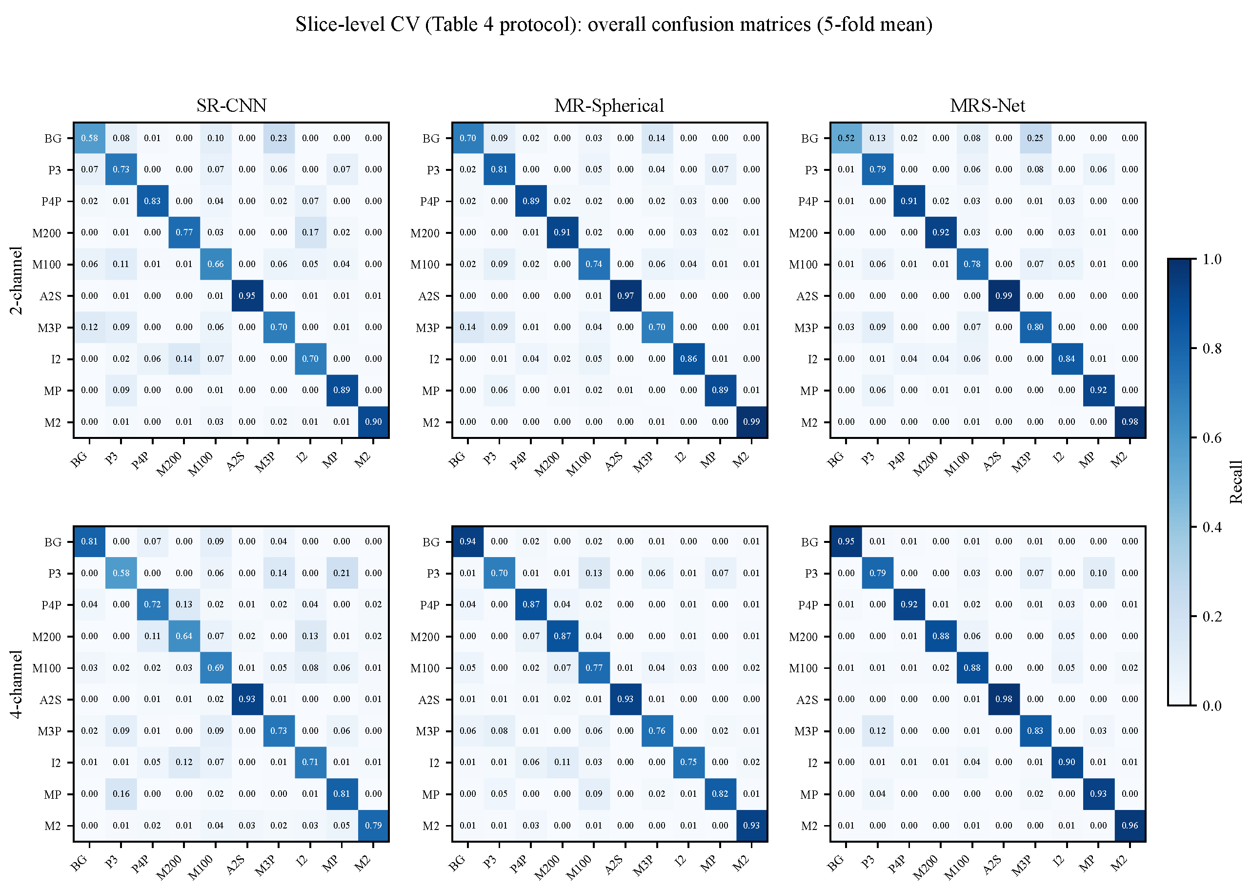
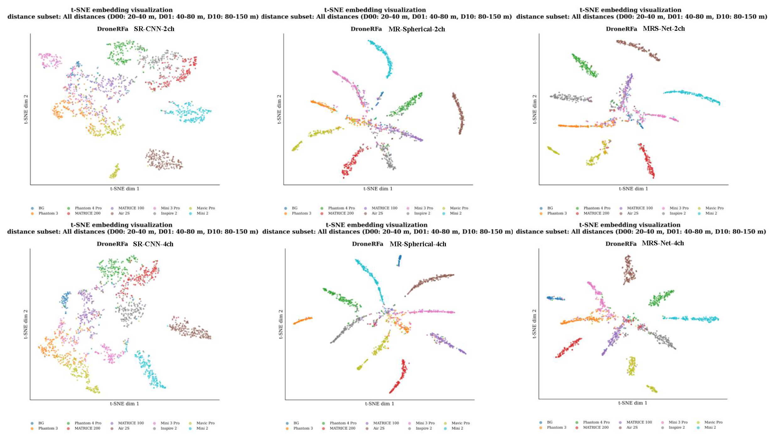
Figure 9 presents, in a $2\times 3$ layout (2ch/4ch by SR-CNN/MR-Spherical/MRS-Net), the class-level confusion matrices for the six settings under real distance attenuation reported in Table 4; the corresponding confusion matrices under the session-level grouped protocol are shown in the Supplementary Materials. Figure 10 shows the corresponding t-distributed stochastic neighbor embedding (t-SNE) visualizations. The MRS-Net embeddings exhibit greater inter-class separation and tighter intra-class distributions, although t-SNE provides qualitative rather than quantitative evidence.

5.3. Complementary Experiment: Cross-Method Comparison on Noisy Drone RF

Noisy Drone RF provides complementary evaluation under explicit additive noise and comparison with representative backbone networks. Table 5 reports BAcc at SNRs from $-20$ dB to $-10$ dB. The “Mean” row averages BAcc over these six reported low-SNR levels, whereas “Overall” denotes BAcc over the complete SNR range from $-20$ dB to 30 dB.

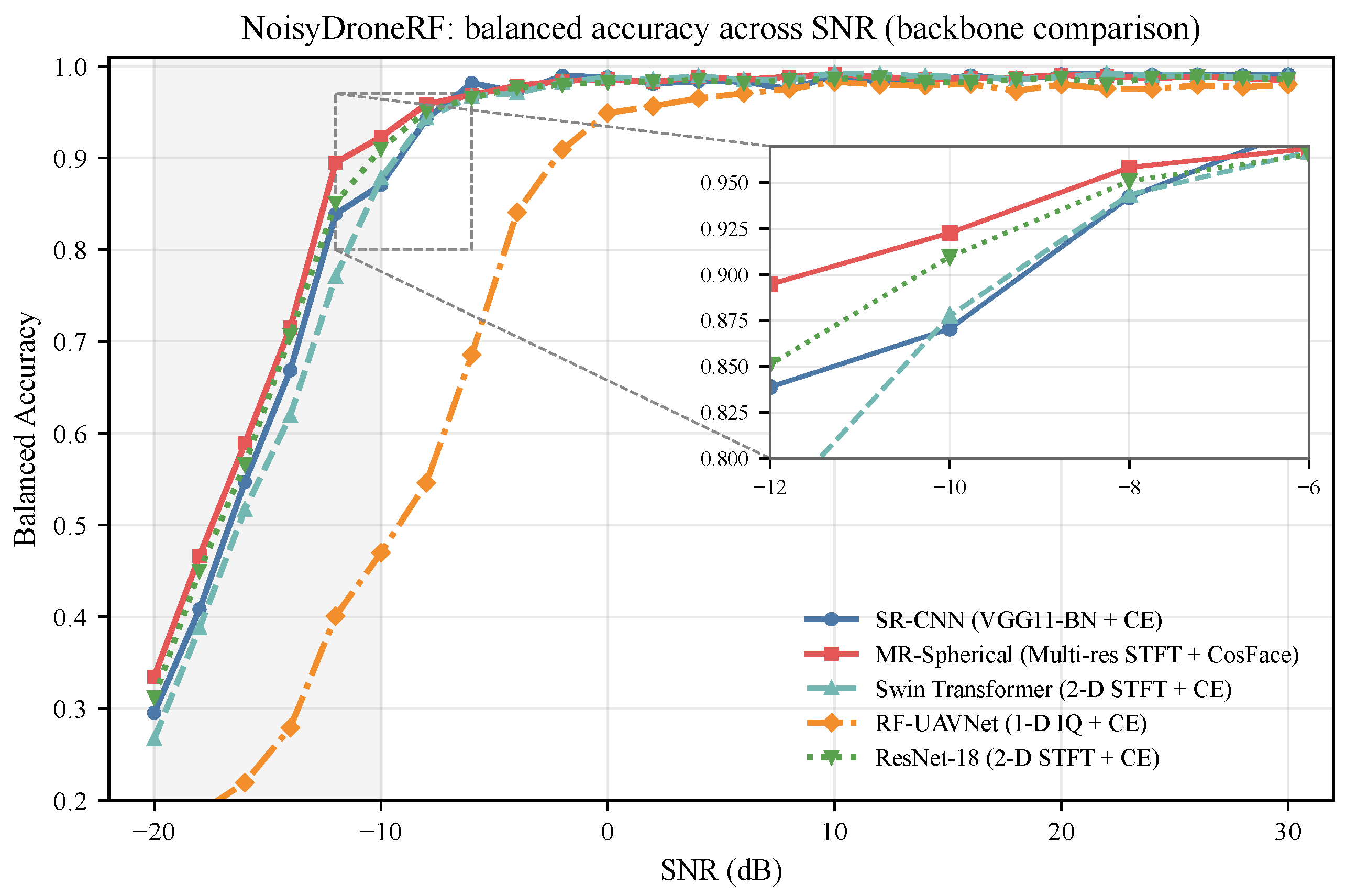
Figure 11 shows the BAcc-versus-SNR curves. From $-20$ dB to $-10$ dB, MR-Spherical achieves a mean BAcc of 65.38%, exceeding SR-CNN by 4.91 pp. MR-Spherical also exceeds SR-CNN at every reported SNR in this interval. These results support the benefit of multi-resolution representation and hyperspherical discrimination under strong additive noise.

Table 5. Cross-method comparison on Noisy Drone RF. “Mean” averages BAcc over the six reported SNR levels from $-20$ dB to $-10$ dB, whereas “Overall” reports BAcc over the full SNR range from $-20$ dB to 30 dB.

SNR (dB)	SR-CNN	MR-Spherical	Swin Transformer	ResNet-18	RF-UAVNet
$-20$	29.54	33.46	26.68	31.23	16.34
$-18$	40.81	46.64	38.79	45.25	18.74
$-16$	54.68	58.90	51.67	56.63	21.95
$-14$	66.84	71.50	61.91	70.56	28.05
$-12$	83.89	89.48	77.06	85.09	39.65
$-10$	87.06	92.28	87.76	91.18	47.08
Mean	60.47	65.38	57.31	63.32	28.64
Overall	89.72 ± 0.22	90.78 ± 0.35	88.92 ± 0.48	90.06 ± 0.43	77.93 ± 1.17

Table 5. Cross-method comparison on Noisy Drone RF. “Mean” averages BAcc over the six reported SNR levels from $-20$ dB to $-10$ dB, whereas “Overall” reports BAcc over the full SNR range from $-20$ dB to 30 dB.

SNR (dB)	SR-CNN	MR-Spherical	Swin Transformer	ResNet-18	RF-UAVNet
$-20$	29.54	33.46	26.68	31.23	16.34
$-18$	40.81	46.64	38.79	45.25	18.74
$-16$	54.68	58.90	51.67	56.63	21.95
$-14$	66.84	71.50	61.91	70.56	28.05
$-12$	83.89	89.48	77.06	85.09	39.65
$-10$	87.06	92.28	87.76	91.18	47.08
Mean	60.47	65.38	57.31	63.32	28.64
Overall	89.72 ± 0.22	90.78 ± 0.35	88.92 ± 0.48	90.06 ± 0.43	77.93 ± 1.17

Comparison with other backbones indicates that network complexity alone does not determine low-SNR RF identification performance. Although Swin Transformer and ResNet-18 perform strongly at some SNRs, MR-Spherical achieves the highest mean BAcc across the reported low-SNR interval. This result supports the importance of both input representation and feature-space constraints. Multi-resolution STFT improves weak-structure observation, while CosFace increases the angular class margin.

5.4. Ablation Studies

Three groups of ablation experiments isolate the contribution of each module and characterize the conditions under which RSP is effective.

5.4.1. Progressive Component Ablation

The comparison between SR-CNN and MR-Spherical measures the joint gain of multi-resolution representation and the hyperspherical constraint. MR-Spherical increases overall BAcc from 77.02% to 84.74% under 2ch input and from 74.01% to 83.20% under 4ch input. Multi-resolution STFT provides complementary observations of narrowband control and broadband video-transmission signals. CosFace enlarges the inter-class angular margin and reduces embedding overlap under low SNR.

Because this comparison changes both the STFT representation and the classification loss at the same time, it does not by itself isolate the contribution of CosFace.

Table 6. Factorial ablation of the STFT representation and the classification loss on DroneRFa (slice-level protocol, mean ± std over 5 folds).

Input	STFT	Cross-Entropy	CosFace
2ch	Single-resolution (SR)	77.02 ± 3.78	81.97 ± 1.68
2ch	Multi-resolution (MR)	80.72 ± 2.42	84.74 ± 0.94
4ch	Single-resolution (SR)	74.01 ± 12.11	77.91 ± 8.40
4ch	Multi-resolution (MR)	83.00 ± 13.28	83.20 ± 16.78

reports a $2\times 2$ factorial ablation, under the same slice-level protocol and hyperparameters as Table 3, that crosses single-resolution (SR) and multi-resolution (MR) STFT with cross-entropy (CE) and CosFace losses; the SR + CE and MR + CosFace rows reproduce the SR-CNN and MR-Spherical entries of Table 4, while SR+CosFace and MR+CE were trained separately to complete the design.

Under 2ch input, both factors contribute positively and are roughly additive: CosFace contributes +4.95 pp with a single-resolution STFT and +4.02 pp with a multi-resolution STFT, while multi-resolution STFT contributes +3.70 pp under cross-entropy and +2.77 pp under CosFace. Under 4ch input, multi-resolution STFT is the dominant factor (+8.99 pp under cross-entropy, +5.29 pp under CosFace), whereas the additional contribution of CosFace once multi-resolution STFT is already present is small (+0.20 pp). RSP is not part of this $2\times 2$ design; its contribution is examined separately below.

The comparison between MR-Spherical and MRS-Net isolates the effect of RSP. Under 2ch input, their overall BAcc values are similar (84.74% and 84.50%), suggesting that the $2\times 2$ SPD matrix formed from single-receiver I/Q carries limited exploitable geometric information. Under 4ch input, MRS-Net exceeds MR-Spherical by 7.10 pp while the cross-fold standard deviation falls from 16.78% to 1.46%; as Section 5.6 shows, the mean gap is fold-sensitive, so we treat the variance reduction as the more robust evidence for RSP. This benefit is therefore concentrated in the multi-channel setting, where $4\times 4$ SPD matrices encode richer cross-receiver correlations.

5.4.2. Parameter-Aligned Ablation of Multi-Resolution STFT

To isolate the effect of multi-resolution STFT, we conduct a parameter-aligned ablation on Noisy Drone RF. All variants use CosFace and differ only in STFT resolution and branch count. Table 7 reports the results. Overall, BAcc follows the same full-range definition from $-20$ dB to 30 dB.

The results indicate that the gain does not arise solely from additional parameters. A1 has the same branch count and a similar parameter count as MR-Spherical, yet MR-Spherical achieves higher low-SNR BAcc. Complementary STFT resolutions therefore contribute information beyond model capacity. The strong performance of the single-branch A3 also highlights the importance of frequency resolution for narrowband signals. MR-Spherical further improves on A3 by combining high temporal resolution, an intermediate time-frequency resolution, and high frequency resolution.

Table 7. Parameter-aligned ablation results of multi-resolution STFT.

Experiment	STFT Config	Loss	Branches	Overall BAcc (%)	Low-SNR BAcc (%)
SR-CNN	$N_{\mathrm{fft}}=256$	CE	1	89.72 ± 0.22	60.47
A2	$N_{\mathrm{fft}}=128$	CosFace	1	89.47 ± 0.31	59.58
A3	$N_{\mathrm{fft}}=512$	CosFace	1	90.49 ± 0.41	64.80
A4	$N_{\mathrm{fft}}=\{128,256\}$	CosFace	2	90.21 ± 0.41	63.14
A5	$N_{\mathrm{fft}}=\{256,512\}$	CosFace	2	90.41 ± 0.22	62.71
A1	$3\times N_{\mathrm{fft}}=256$	CosFace	3	90.49 ± 0.40	63.84
MR-Spherical	$N_{\mathrm{fft}}=\{128,256,512\}$	CosFace	3	90.78 ± 0.35	65.38

Table 7. Parameter-aligned ablation results of multi-resolution STFT.

Experiment	STFT Config	Loss	Branches	Overall BAcc (%)	Low-SNR BAcc (%)
SR-CNN	$N_{\mathrm{fft}}=256$	CE	1	89.72 ± 0.22	60.47
A2	$N_{\mathrm{fft}}=128$	CosFace	1	89.47 ± 0.31	59.58
A3	$N_{\mathrm{fft}}=512$	CosFace	1	90.49 ± 0.41	64.80
A4	$N_{\mathrm{fft}}=\{128,256\}$	CosFace	2	90.21 ± 0.41	63.14
A5	$N_{\mathrm{fft}}=\{256,512\}$	CosFace	2	90.41 ± 0.22	62.71
A1	$3\times N_{\mathrm{fft}}=256$	CosFace	3	90.49 ± 0.40	63.84
MR-Spherical	$N_{\mathrm{fft}}=\{128,256,512\}$	CosFace	3	90.78 ± 0.35	65.38

5.4.3. Backbone Generalization Ablation

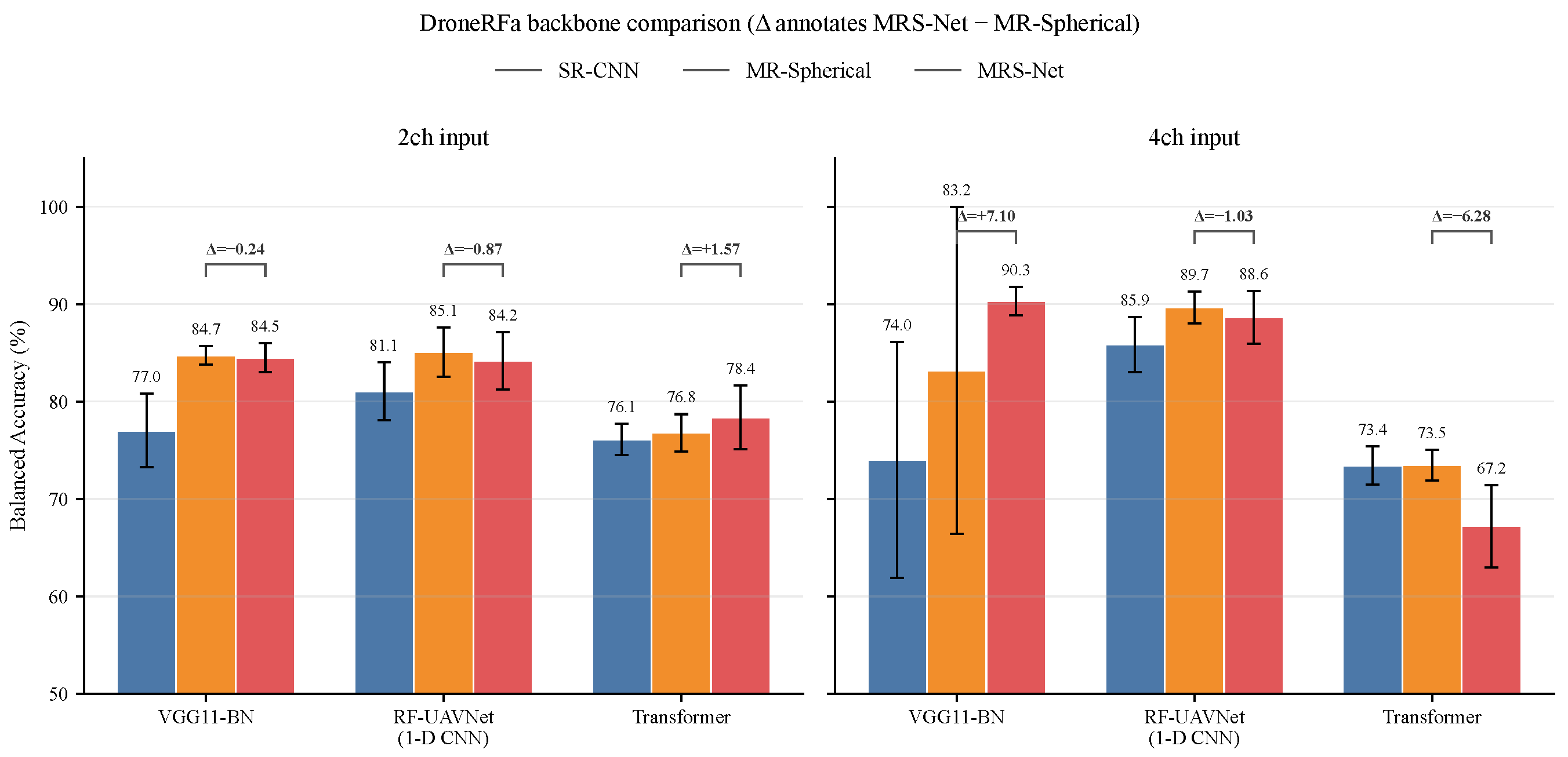
To test whether the MRS-Net gains depend on VGG11-BN, we replace it with ConvStem-Transformer and RF-UAVNet [14], a published one-dimensional CNN baseline for RF-based drone identification, as backbones, which also lets this comparison serve as an external-baseline check under our own training protocol. We compare SR-CNN, MR-Spherical, and MRS-Net under the same DroneRFa protocol, using identical cropping, the same slice-level 5-fold splits as Table 4, the same RMS normalization, and the same sampling length.

Table 8. Backbone generalization results on DroneRFa, with RSP’s independent contribution isolated via $\Delta$(MRS-Net−MR-Spherical).

Backbone	Input	SR-CNN	MR-Spherical	MRS-Net	$\Delta$(MRS-Net − MR-Spherical)	$\Delta$(MRS-Net − SR-CNN)
Transformer	2ch	76.11	76.80	78.37	+1.57	+2.26
Transformer	4ch	73.43	73.49	67.21	$-6.28$	$-6.22$
RF-UAVNet (1-D CNN)	2ch	81.07	85.07	84.20	$-0.87$	+3.13
RF-UAVNet (1-D CNN)	4ch	85.86	89.67	88.63	$-1.04$	+2.77
VGG11-BN	2ch	77.02	84.74	84.50	$-0.24$	+7.48
VGG11-BN	4ch	74.01	83.20	90.30	+7.10	+16.29

and Figure 12 report the results, including a $\Delta$(MRS-Net−MR-Spherical) column that isolates the independent contribution of RSP from the joint multi-resolution-STFT-plus-CosFace effect captured by $\Delta$(MRS-Net−SR-CNN).

The results are best read through the $\Delta$(MRS-Net−MR-Spherical) column, which isolates the contribution of RSP from the multi-resolution-STFT-plus-CosFace effect already captured by $\Delta$(MRS-Net−SR-CNN). On this basis, RSP’s contribution is positive only for VGG11-BN-4ch (+7.10 pp; see Section 5.6 for the caveats on this figure), essentially flat for VGG11-BN-2ch ($-0.24$ pp) and for RF-UAVNet-2ch/4ch ($-0.87$/$-1.04$ pp), and clearly negative for Transformer-4ch ($-6.28$ pp). MRS-Net is therefore not restricted to VGG11-BN: with RF-UAVNet as the backbone, the complete framework exceeds SR-CNN under both 2ch and 4ch input. However, MRS-Net underperforms its MR-Spherical counterpart with the Transformer backbone and 4ch input, showing that RSP is not universally compatible with arbitrary backbones. RSP is therefore not a backbone-agnostic accuracy booster; because the RSP teacher signal is derived from local SPD covariance, it is better matched to extractors that preserve local time-frequency or temporal structure together with sufficiently rich cross-channel covariance. The globally oriented Transformer embedding does not align well with this local constraint under 4ch input, and the same is true, to a smaller degree, of RF-UAVNet’s one-dimensional convolutional structure.

5.5. Deployment and Complexity Analysis

RSP computes local SPD statistics and the similarity-alignment loss only during training and is removed at inference. MRS-Net and MR-Spherical, therefore, share the same backbone structure and nearly identical inference complexity.

Table 9. Inference cost and deployment analysis. Italicized “2ch” and “4ch” label the row blocks for two-channel (single-receiver I/Q) and four-channel (dual-receiver I/Q) input, respectively.

Model	Parameters (M)	Inference Time (ms/Sample)	Throughput (Samples/s)
2ch
SR-CNN	9.359	12.734	78.53
MR-Spherical	28.072	31.438	31.83
MRS-Net	28.072	31.971	31.28
4ch
SR-CNN	9.360	10.986	91.03
MR-Spherical	28.076	34.226	29.22
MRS-Net	28.076	33.748	29.63

reports parameter counts, single-sample inference times, and throughput.

The three-branch multi-resolution structure is the main source of inference overhead. CosFace changes only the classification head and adds negligible inference cost, while RSP adds no online computation. SR-CNN or MR-Spherical may be better suited to resource-constrained real-time deployment. MRS-Net-4ch is more appropriate for fixed multi-receiver stations that prioritize robustness under long-range, low-quality conditions.

5.6. Discussion

Under the slice-level, in-session protocol of Table 4, MRS-Net-4ch achieves the strongest overall BAcc, distance-wise BAcc, and cross-fold stability among the tested DroneRFa configurations, supporting the combined use of multi-resolution representation, CosFace, and RSP under matched acquisition conditions. Multi-resolution STFT and CosFace also improve low-SNR performance on both Noisy Drone RF and DroneRFa: the factorial ablation in Table 6 shows that both factors contribute under 2ch input, while multi-resolution STFT dominates under 4ch input. The benefit of RSP itself is more conditional. It depends on a sufficiently rich multi-channel covariance structure and on a backbone that preserves local time-frequency structure (Table 8), and it is most evident with 4ch dual-receiver input and VGG11-BN but flat or negative with 2ch input, RF-UAVNet, or the Transformer backbone.

This conditional pattern motivated two further checks on how much the RSP result depends on the data split and the random seed. Session-level grouped cross-validation, which forbids slices from the same recording session from appearing on both sides of a fold, lowers overall BAcc for all six configurations (Supplementary Materials): to $53.56\%\pm 10.18\%$/$64.78\%\pm 7.84\%$/$67.27\%\pm 6.82\%$ for SR-CNN/MR-Spherical/MRS-Net on 2ch input, and to $60.96\%\pm 9.40\%$/$60.08\%\pm 14.85\%$/$60.23\%\pm 13.41\%$ on 4ch input. Multi-resolution STFT and CosFace remain positive relative to SR-CNN on 2ch input under this stricter protocol, but on 4ch input the MRS-Net-minus-MR-Spherical gap falls to about $+0.15$ percentage points, so the 4ch advantage seen under the in-session protocol does not persist under cross-session evaluation. Repeating the 4ch slice-level training with two additional seeds (123 and 2024, same fixed folds) confirms that the single-fold collapse of MR-Spherical-4ch at seed 42 is not a general pattern: it does not recur at either additional seed, and the mean MRS-Net-minus-MR-Spherical difference is seed-dependent, ranging from a small negative to a small positive value across the three seeds (Supplementary Materials).

We accordingly restrict the claim for RSP to three points: it reduces the cross-fold standard deviation under 4ch input on the evaluated slice-level run; this stability benefit is not guaranteed to reproduce identically across random seeds or to persist under session-level cross-validation; and its effect is backbone- and channel-dependent, turning negative for the Transformer backbone and for RF-UAVNet (Table 8). We do not claim a generally reproducible mean-accuracy gain from RSP, and none of these findings extend to unseen recording sessions, unseen hardware, unseen interference types, or open-set UAV classes, which lie outside the scope of the present evaluation.

Overall, the results match the intended roles of the three modules. Multi-resolution representation mitigates the limits of a single time-frequency scale, CosFace reduces low-SNR embedding overlap, and RSP exploits local multi-channel SPD statistics to improve structural stability under the evaluated in-session, multi-channel configuration, subject to the seed- and protocol-dependence noted above. Together they address weak-signal observation, embedding discrimination, and structural-prior utilization.

6. Conclusions

We propose MRS-Net for robust drone RF identification under low SNR, long-range attenuation, and multi-channel reception. Its RSP mechanism transfers local SPD covariance relationships into CNN embeddings through pairwise similarity alignment, multi-resolution STFT improves weak-signal observation, and CosFace enlarges angular class margins, combining signal-derived structural supervision with discriminative representation learning.

On DroneRFa, MRS-Net reaches 90.30% overall BAcc with 4ch input under the slice-level, in-session protocol of Table 4, improving BAcc at 80–150 m from 61.30% (SR-CNN-4ch) to 78.30% and reducing the 5-fold standard deviation from 16.78% to 1.46% relative to MR-Spherical-4ch. Complementary experiments under additive noise support the multi-resolution and CosFace contributions independently of the fold, seed, or backbone tested. The evidence for RSP is more limited: its mean-accuracy gain over MR-Spherical is not established as a robust effect, since it depends on a single difficult fold, is seed-dependent, does not persist under session-level cross-validation, and turns flat or negative for the Transformer backbone, RF-UAVNet, and 2ch input. We therefore restrict the robustness claim for RSP to a reduction in cross-fold training variability under 4ch, VGG11-BN-based training on the evaluated protocol, rather than a general improvement in mean accuracy.

None of the reported results are evaluated on unseen recording sessions, receiver hardware, interference types, or open-set UAV classes. Future work will examine lighter backbones, richer propagation information, and more complex interference and open-set conditions.

References

1. Rahman, M.H.; Sejan, M.A.S.; Aziz, M.A.; Tabassum, R.; Baik, J.-I.; Song, H.-K. A Comprehensive Survey of Unmanned Aerial Vehicles Detection and Classification Using Machine Learning Approach: Challenges, Solutions, and Future Directions. Remote Sens. 2024, 16, 879. [Google Scholar] [CrossRef] [Scilit]
2. Li, C.J.; Ling, H. An Investigation on the Radar Signatures of Small Consumer Drones. IEEE Antennas Wirel. Propag. Lett. 2016, 16, 649–652. [Google Scholar] [CrossRef] [Scilit]
3. Jian, M.; Lu, Z.; Chen, V.C. Drone Detection and Tracking Based on Phase-Interferometric Doppler Radar. In Proceedings of the 2018 IEEE Radar Conference (RadarConf18), Oklahoma City, OK, USA, 23–27 April 2018; pp. 1146–1149. [Google Scholar] [CrossRef] [Scilit]
4. Liang, C.; Cao, N.; Lu, X.; Ye, Y. UAV Detection Using Continuous Wave Radar. In Proceedings of the 2018 IEEE International Conference on Information Communication and Signal Processing (ICICSP), Singapore, 28–30 September 2018; pp. 1–5. [Google Scholar] [CrossRef] [Scilit]
5. Nan, H.; Fei, Y.; Yuan, L.; Yang, L.; Chao, L.; Shan, H.; Wei, B. A Lightweight Feature Enhancement Model for UAV Detection in Real-World Scenarios. Drones 2025, 9, 874. [Google Scholar] [CrossRef] [Scilit]
6. Anwar, M.Z.; Kaleem, Z.; Jamalipour, A. Machine Learning Inspired Sound-Based Amateur Drone Detection for Public Safety Applications. IEEE Trans. Veh. Technol. 2019, 68, 2526–2534. [Google Scholar] [CrossRef] [Scilit]
7. Yaacoub, M.; Younes, H.; Rizk, M. Acoustic Drone Detection Based on Transfer Learning and Frequency Domain Features. In Proceedings of the 2022 International Conference on Smart Systems and Power Management (IC2SPM), Beirut, Lebanon, 10–12 November 2022; pp. 47–51. [Google Scholar] [CrossRef] [Scilit]
8. Jeon, S.; Shin, J.W.; Lee, Y.J.; Kim, W.H.; Kwon, Y.; Yang, H.Y. Empirical Study of Drone Sound Detection in Real-Life Environment with Deep Neural Networks. In Proceedings of the 2017 25th European Signal Processing Conference, Kos, Greece, 28 August–2 September 2017; pp. 1858–1862. [Google Scholar] [CrossRef] [Scilit]
9. Shi, Y.; Shan, T.; Dong, H. Integrated Detection of Weak Drone Signals: From Parameter Estimation to Sensitive Classification. Digit. Signal Process. 2026, 168, 105524. [Google Scholar] [CrossRef] [Scilit]
10. Yousaf, J.; Zia, H.; Alhalabi, M.; Yaghi, M.; Basmaji, T.; Shehhi, E.A.; Gad, A.; Alkhedher, M.; Ghazal, M. Drone and Controller Detection and Localization: Trends and Challenges. Appl. Sci. 2022, 12, 12612. [Google Scholar] [CrossRef] [Scilit]
11. Al-Emadi, S.; Al-Senaid, F. Drone Detection Approach Based on Radio-Frequency Using Convolutional Neural Network. In Proceedings of the 2020 IEEE International Conference on Informatics, IoT, and Enabling Technologies (ICIoT), Doha, Qatar, 2–5 February 2020; pp. 29–34. [Google Scholar] [CrossRef] [Scilit]
12. Allahham, M.S.; Khattab, T.; Mohamed, A. Deep Learning for RF-Based Drone Detection and Identification: A Multi-Channel 1-D Convolutional Neural Networks Approach. In Proceedings of the 2020 IEEE International Conference on Informatics, IoT, and Enabling Technologies (ICIoT), Doha, Qatar, 2–5 February 2020; pp. 112–117. [Google Scholar] [CrossRef] [Scilit]
13. Mandal, S.; Satija, U. Time-Frequency Multiscale Convolutional Neural Network for RF-Based Drone Detection and Identification. IEEE Sens. Lett. 2023, 7, 7003304. [Google Scholar] [CrossRef] [Scilit]
14. Huynh-The, T.; Pham, Q.V.; Nguyen, T.V.; da Costa, D.B.; Kim, D.S. RF-UAVNet: High-Performance Convolutional Network for RF-Based Drone Surveillance Systems. IEEE Access 2022, 10, 49696–49707. [Google Scholar] [CrossRef] [Scilit]
15. Al-Sa’d, M.F.; Al-Ali, A.; Mohamed, A.; Khattab, T.; Erbad, A. RF-Based Drone Detection and Identification Using Deep Learning Approaches: An Initiative towards a Large Open Source Drone Database. Future Gener. Comput. Syst. 2019, 100, 86–97. [Google Scholar] [CrossRef] [Scilit]
16. Ge, J.; Zhang, H.; Li, J.; Wen, Z. One-Step Framework for RF-Based Drone Identification. In Proceedings of the 2024 5th International Conference on Computer Vision, Image and Deep Learning (CVIDL), Zhuhai, China, 19–21 April 2024; pp. 919–925. [Google Scholar] [CrossRef] [Scilit]
17. Sazdic-Jotic, B.; Andric, M.; Bondzulic, B.; Simic, S.; Pokrajac, I. FLEDNet: Enhancing the Drone Classification in the Radio Frequency Domain. Drones 2025, 9, 243. [Google Scholar] [CrossRef] [Scilit]
18. Wang, S.; Luo, Y.; Zheng, Y.; Sun, Z.; Zheng, Y.; Liu, T.; Jin, Z. Detection and Recognition of UAV Radio Frequency Signals Based on Time-Frequency Processing and Transfer Learning with Multi-Channel Input. Signal Image Video Process. 2025, 19, 868. [Google Scholar] [CrossRef] [Scilit]
19. Xue, C.; Li, T.; Li, Y.; Ruan, Y.; Zhang, R.; Dobre, O.A. Radio-Frequency Identification for Drones with Nonstandard Waveforms Using Deep Learning. IEEE Trans. Instrum. Meas. 2023, 72, 5503713. [Google Scholar] [CrossRef] [Scilit]
20. Zhang, H.; Li, T.; Li, Y.; Li, J.; Dobre, O.A.; Wen, Z. RF-Based Drone Classification under Complex Electromagnetic Environments Using Deep Learning. IEEE Sens. J. 2023, 23, 6099–6108. [Google Scholar] [CrossRef] [Scilit]
21. Cai, Z.; Wang, Y.; Jiang, Q.; Gui, G.; Sha, J. Toward Intelligent Lightweight and Efficient UAV Identification with RF Fingerprinting. IEEE Internet Things J. 2024, 11, 26329–26339. [Google Scholar] [CrossRef] [Scilit]
22. Cai, Z.; Wang, Y.; Gui, G.; Sha, J. Toward Robust Radio Frequency Fingerprint Identification via Adaptive Semantic Augmentation. IEEE Trans. Inf. Forensics Secur. 2025, 20, 1037–1048. [Google Scholar] [CrossRef] [Scilit]
23. Wang, H.; Wang, Y.; Zhou, Z.; Ji, X.; Gong, D.; Zhou, J.; Li, Z.; Liu, W. CosFace: Large Margin Cosine Loss for Deep Face Recognition. In Proceedings of the IEEE/CVF Conference on Computer Vision and Pattern Recognition, Salt Lake City, UT, USA, 18–22 June 2018; pp. 5265–5274. [Google Scholar] [CrossRef] [Scilit]
24. Wang, H.; Yang, S.; Feng, Z. SSME: A Semi-Supervised Specific Emitter Identification Method with Manifold Enhancement. IEEE Trans. Inf. Forensics Secur. 2025, 20, 10161–10172. [Google Scholar] [CrossRef] [Scilit]
25. Yang, Z.; Cheng, Y.; Wu, H.; Liu, K.; Wang, H.; Qin, Y. Correlation-Feature-Based Information Geometry Detection for Weak Motion Target in Complex Environment. IEEE Internet Things J. 2025, 12, 11926–11939. [Google Scholar] [CrossRef] [Scilit]
26. Wu, H.; Cheng, Y.; Chen, X.; Yang, Z.; Li, X.; Wang, H. Geodesic Normal Coordinate-Based Manifold Filtering for Target Detection. IEEE Trans. Geosci. Remote Sens. 2022, 60, 5114615. [Google Scholar] [CrossRef] [Scilit]
27. Yu, N.; Mao, S.; Zhou, C.; Sun, G.; Shi, Z.; Chen, J. DroneRFa: A Large-Scale Dataset of Drone Radio Frequency Signals for Detecting Low-Altitude Drones. J. Electron. Inf. Technol. 2024, 46, 1147–1156. [Google Scholar] [CrossRef]
28. Glüge, S.; Nyfeler, M.; Aghaebrahimian, A.; Ramagnano, N.; Schüpbach, C. Robust Low-Cost Drone Detection and Classification Using Convolutional Neural Networks in Low SNR Environments. IEEE J. Radio Freq. Identif. 2024, 8, 821–830. [Google Scholar] [CrossRef] [Scilit]
Figure 1. Representative time-frequency spectrograms of a UAV RF signal at SNRs of 20 dB and 10 dB. Under low SNR, the amplitude texture is strongly contaminated by noise, while the local covariance structure may still preserve part of the signal correlation.
Drones 10 00709 g001
Figure 2. Representative time-frequency spectrograms of UAV RF signals. Background color encodes the relative spectral power at each time–frequency bin (dark blue: low power; yellow/red: high power). Red, blue, orange, and green boxes mark broadband video-transmission bursts, narrowband remote-control signals, Wi-Fi interference, and Bluetooth signals, respectively. These structures motivate the use of complementary time-frequency scales.
Drones 10 00709 g002
Figure 3. Riemannian distance maps (RDM) of two representative UAV classes (DJI Phantom 3 and DJI Phantom 4 Pro) under D00 (20–40 m), D01 (40–80 m), and D10 (80–150 m). Brighter colors indicate a larger geometric deviation d LE of the local SPD covariance structure from the noise-reference SPD centroid.
Drones 10 00709 g003
Figure 4. Local-variation-gradient fields κ of the same UAV classes and distance conditions. Background color encodes the magnitude of local geometric variation κ (a first-order finite-difference quantity, not a differential-geometric curvature), and arrows indicate the local direction of geometric variation in the log-domain SPD field.
Drones 10 00709 g004
Figure 5. Log-determinant responses tr ( log Σ ) of the same UAV classes and distance conditions. The block-wise heat maps represent the volume or energy spread of the local covariance matrices.
Drones 10 00709 g005
Figure 6. Normalized mean profile of five representative UAV classes across 13 key Riemannian statistical dimensions, including the RDM and local-variation statistics at three STFT scales and their cross-scale ratios. Where two classes’ trajectories nearly coincide along a given axis (e.g., DJI Matrice 200 overlapping with Background or DJI Phantom 3), the classes share a similar value on that specific statistic; such local overlap does not by itself imply overall class confusability, which depends on the joint 13-dimensional profile rather than any single axis.
Drones 10 00709 g006
Figure 7. Overall MRS-Net pipeline. Multi-resolution time-frequency representations of the raw I/Q segment are encoded by parallel CNN branches and fused into a unified embedding supervised by CosFace. RSP provides training-only structural supervision and is removed at inference.
Drones 10 00709 g007
Figure 8. Distance-wise balanced accuracy comparison on DroneRFa. D00, D01, and D10 correspond to 20–40 m, 40–80 m, and 80–150 m, respectively.
Drones 10 00709 g008
Figure 9. Confusion matrices for the six DroneRFa settings in a 2 × 3 layout (rows: 2-channel/4-channel; columns: SR-CNN/MR-Spherical/MRS-Net). Each panel is the 5-fold-mean confusion matrix for that setting under the slice-level protocol of Table 4.
Drones 10 00709 g009
Figure 10. t-SNE visualizations of the learned DroneRFa embeddings, showing the clustering and inter-class separation of the six experimental settings.
Drones 10 00709 g010
Figure 11. Balanced accuracy of different methods versus SNR on Noisy Drone RF. The MR-Spherical curve corresponds to the MR-Spherical row of Table 5; RSP is not used in this experiment (Table 2 lists RSP as not applicable on Noisy Drone RF).
Drones 10 00709 g011
Figure 12. Backbone replacement comparison on DroneRFa. VGG11-BN is replaced by ConvStem-Transformer or RF-UAVNet (1-D CNN) to evaluate the transferability of the multi-resolution and RSP designs; MRS-Net and MR-Spherical are grouped to highlight RSP’s independent contribution.
Drones 10 00709 g012