GeoRefGS: Towards Georeferenced 3D Gaussian Splatting from Unmanned Aerial Vehicle Platforms

Highlights

What are the main findings?

• We design a geographic loss function to embed georeferencing constraints directly into high-fidelity 3D Gaussian Splatting.
• We introduce a learnable similarity transformation matrix T as the key bridge to align the model with the global geographic coordinate system during training.

What are the implications of the main findings?

• This work enables 3D Gaussian Splatting to produce models with accurate geographic coordinates, unlocking its potential for professional applications like digital twins, environmental monitoring, and smart cities.
• Introducing a similarity transformation matrix along with geographic loss functions effectively mitigates potential issues such as gradient explosion or training instability caused by excessively large coordinate values, enabling rapid convergence.

Abstract

Three-dimensional reconstruction using unmanned aerial vehicle (UAV) platforms has been extensively utilized in various fields. While conventional techniques such as oblique photogrammetry can produce mesh models with geographical references, they often require substantial computational resources. Although recent studies have attempted to incorporate camera pose parameters into the emerging 3D Gaussian Splatting (3DGS), these methods often treat georeferencing as a post-processing step or rely on global bundle adjustment, which may propagate systematic errors and compromise final accuracy. This work integrates georeferencing as an intrinsic constraint during 3DGS training, enabling simultaneous optimization of geographic and photometric accuracy. The core of our approach lies in introducing a similarity transformation matrix T connecting the local model space with the global geographic coordinate system, along with a dedicated geographic loss function. Geographic coordinates are transformed via T before reprojection to compute the loss function. It was demonstrated that GeoRefGS presents a viable solution for efficiently integrating georeferenced information into 3DGS. Indeed, the proposed framework achieves an improvement of approximately 3.31 dB in peak signal-to-noise ratio while maintaining distance errors below 0.054 m, enabling reliable geographically referenced 3D reconstruction in substantially less time compared to conventional photogrammetric approaches.

1. Introduction

Three-dimensional reconstruction based on unmanned aerial vehicle (UAV) platforms was initially employed primarily in the fields of topographic mapping and cartography [1]. Over the past decade, UAV has evolved into a common platform for 3D reality modeling in fields such as digital twins [2], smart cities [3,4], and cultural heritage preservation [5,6]. Compared to conventional methods like terrestrial surveying or airborne laser scanning, UAV photogrammetry offers significant advantages in terms of cost-effectiveness, data acquisition efficiency, and accessibility to complex terrain, while maintaining comparable accuracy and reliability. Consequently, the adoption of three-dimensional reconstruction based on UAV has become increasingly prevalent in various domains, including civil engineering, agricultural remote sensing, environmental monitoring and military reconnaissance [7].

Sequential images acquired by UAVs provide a rich data source for the aforementioned applications [8]. The core of traditional 3D reconstruction relies on Structure-from-Motion (SfM) [9] and Multi-View Stereo (MVS) algorithms [10], enabling the automatic reconstruction of 3D geometry from 2D images. To achieve high-quality results, especially in scenes with weak textures or complex structures, key parameters such as feature matching accuracy and camera pose estimation must be strictly controlled [11]. The generated photogrammetric models, such as point clouds, meshes, and orthophotos, are subsequently integrated into a global coordinate system through a georeferencing process [12]. Conventional georeferencing workflows primarily depend on two main approaches: one is the Ground Control Point-based method [13]; the other is Direct Georeferencing, which replaces ground control points (GCPs) with aerial control by employing GNSS-assisted Bundle Block Adjustment [8] and Automatic Aerial Triangulation [14]. Traditional 3D reconstruction often suffers from low efficiency and poor accuracy when dealing with complex scenes. A common manifestation is the presence of holes in the final models, primarily caused by missing corresponding viewpoint images, which leads to suboptimal results.

The limitations of conventional pipelines have catalyzed a shift in 3D reconstruction, driven by deep learning [15]. This transformation is exemplified by the emergence of novel implicit or explicit scene representations, notably Neural Radiance Fields (NeRF) [16] and 3D Gaussian Splatting (3DGS) [17]. These approaches can generate photorealistic 3D scenes from only sparse 2D image inputs [18]. Fundamentally, NeRF represents a scene implicitly through a multilayer perceptron (MLP) that encodes a continuous volumetric field. This field maps a 3D location and viewing direction to density and view-dependent color [19], enabling photorealistic novel view synthesis via differentiable volume rendering. Addressing practical challenges such as high computational resource consumption and difficulties in scaling to large scenes, researchers have proposed a series of optimization strategies for NeRF. For instance, partitioning the scene into local blocks for independent training reduces memory usage, while fusion mechanisms help maintain overall reconstruction quality [20,21]. Other methods focus on specific applications like aerial photography, employing modular modeling based on spatial structure and camera distribution [22], or introducing autonomous capture strategies to iteratively refine reconstruction [23]. A limited number of studies have begun to explore georeferenced NeRF representations, for example, by incorporating geographic coordinates into positional encoding or introducing projective constraints to establish geospatial consistency [21].

Although a few studies have begun to explore geospatial awareness for NeRF [24], existing methods primarily focus on enhancing rendering quality rather than geolocation accuracy. Furthermore, as an implicit reconstruction method, NeRF still exhibits several notable limitations [25]. Compared to traditional 3D reconstruction, its process and results lack an intuitive, explicit structural representation, making direct observation or physical simulation difficult [26]. Additionally, the generalization capability of current methods is limited, typically with one network being applicable only to one or a very limited number of scenes [27,28]. These technical constraints pose significant challenges and limitations to the development of NeRF for applications requiring strong real-time performance, such as environmental modeling, navigation, and path planning.

As an emerging rendering technique, 3DGS offers significant advantages in computational and rendering efficiency compared to methods like traditional NeRF, owing to its explicit scene representation and parallelizable workflow, enabling high-quality image synthesis. This makes it particularly suitable for real-time and efficient 3D reconstruction following rapid UAV data acquisition [29]. Subsequent research has further enhanced 3DGS, with proposed strategies addressing dynamic objects, geometric fidelity [30], and large-scale reconstruction [31,32] demonstrating compelling performance on public benchmarks. However, despite the continuous emergence of these enhanced methods, 3DGS typically requires input images with unknown camera parameters, relying on SFM to reconstruct sparse point clouds and camera poses from multi-view images. As a result, the generated models are usually constructed within a non-georeferenced local coordinate system. This fundamental disconnect, which we refer to as the “visual–geospatial gap,” hinders the direct application of these high-fidelity models in any domain requiring precise geospatial reasoning and measurement.

It is worth noting that both academia and industry have begun to explore viable pathways for integrating geospatial information into 3DGS. For instance, GeomGS [33] proposes a LiDAR-guided geometry-aware 3DGS method. It deeply integrates LiDAR data into Gaussian primitives through probabilistic constraints, significantly enhancing geometric accuracy for robot localization. However, its core objective is improving local geometric structure, and its reliance on LiDAR sensors limits its applicability in pure vision-based UAV photogrammetry scenarios. On the other hand, industrial practices offer valuable insights. The commercial solution from Mapmost demonstrates key functionalities such as geographic coordinate recovery and 3D spatial measurement, proving the substantial application potential of georeferenced 3DGS in digital twins. Nevertheless, as a proprietary solution, its specific implementation details, especially how geographic constraints are integrated into the 3DGS optimization process, remain unclear.

Images collected by drones can directly provide flight trajectory information [34], offering initial camera extrinsic parameters. However, using drone track points directly as camera extrinsics may lead to mismatches between intrinsic and extrinsic parameters. Therefore, this study aims to propose and validate GeoRefGS, a framework designed for UAV platforms that efficiently embeds georeferencing information into the 3D Gaussian representation. In contrast to these works, the GeoRefGS proposed in this study aims to achieve 3DGS reconstruction on pure vision-based UAV platforms that simultaneously delivers high-fidelity rendering and high geographic accuracy. Compared to GeomGS, our method does not require additional LiDAR sensors. Compared to commercial solutions like Mapmost, GeoRefGS offers a transparent and verifiable academic approach. Its core innovation lies in embedding georeferencing as an intrinsic constraint during training, rather than as a post-processing step. Specifically, we introduce a learnable similarity transformation matrix connecting the local model space with the global geographic coordinate system, integrating georeferencing as an intrinsic constraint during training, and design a geographically consistent optimization strategy to ensure global geometric accuracy. A dedicated geographic loss function is designed to mitigate training instability caused by directly using large-scale geographic coordinates, enabling the joint optimization of geometric and photometric errors.

To rigorously validate the accuracy of the proposed method, a simulation environment was constructed in Unity. Within this virtual setting, an UAV autonomously controlled via ROS2, executed a circular flight trajectory around a building complex to systematically capture multi-view imagery. This controlled setup enabled the precise acquisition of comprehensive image data from all angles. A quantitative evaluation was then performed, comparing the proposed framework against 3DGS. The assessment focused on two key aspects: visual rendering quality, measured by metrics such as Peak Signal-to-Noise Ratio (PSNR) [35] and Structural Similarity Index (SSIM) [36]; and geolocation accuracy, defined as the distance error between reconstructed points and designated ground truth checkpoints.

This study seeks to identify an optimal georeferencing solution for utilizing 3DGS technology in specific applications. GeoRefGS successfully bridges the gap between high-fidelity Gaussian Splatting scene representation and geospatial accuracy. The resulting models can be directly applied to cutting-edge applications such as digital twins and smart cities that require truly 3D, measurable, and analyzable data foundations, with potential for replication in other scenarios with comparable characteristics.

2. Materials and Methods

2.1. Framework

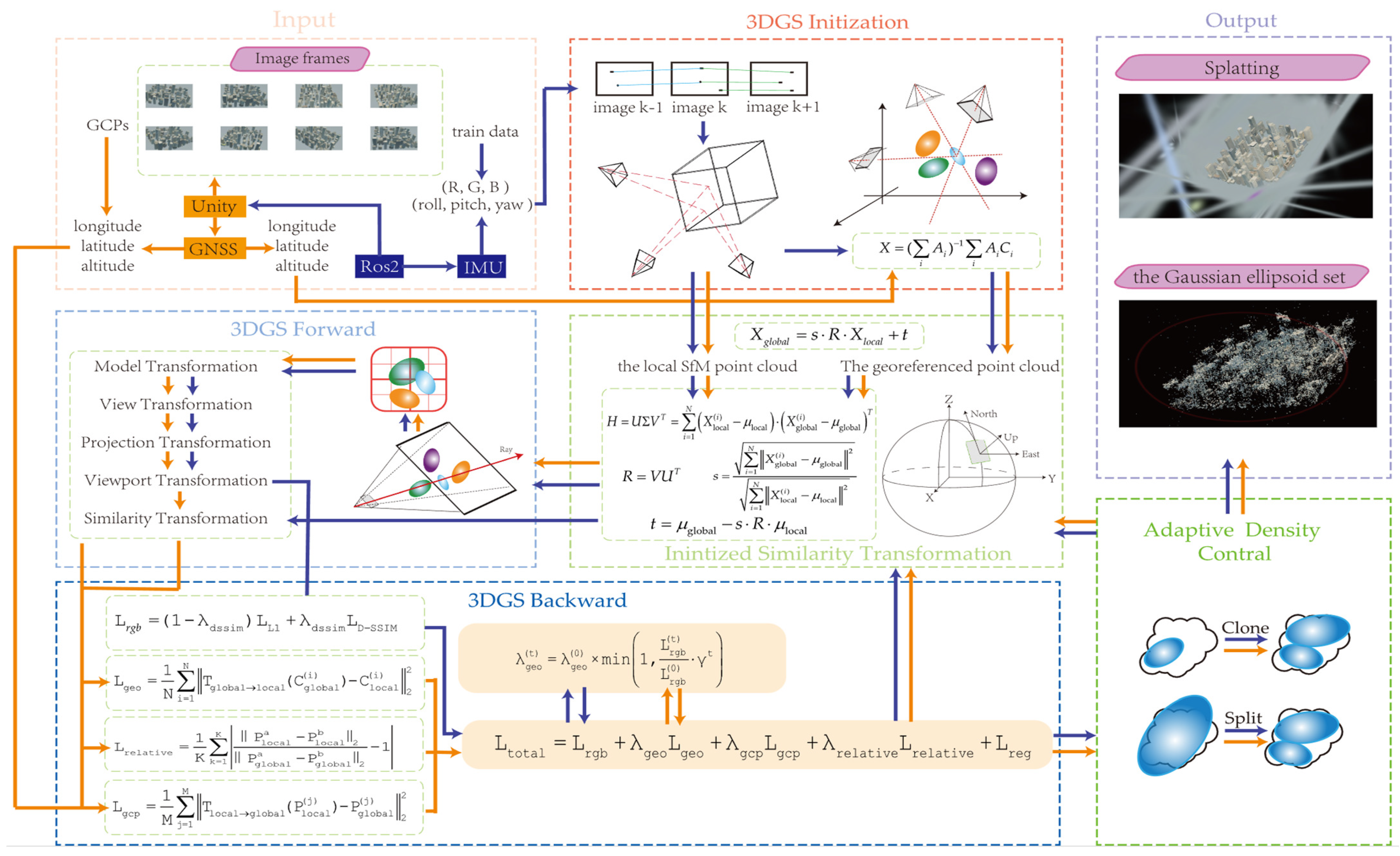
The overall workflow of the GeoRefGS framework is depicted in Figure 1. The system operates through the following pipeline: flight trajectory information is first obtained from the ROS2-controlled UAV system, while synchronized RGB images corresponding to each pose are captured from the Unity simulation environment. These multi-view images are then organized into a dataset and split into training and testing sets. The training set serves as the input to the GeoRefGS model, which processes it to produce a high-fidelity 3D Gaussian scene representation endowed with absolute geographic coordinates. Finally, the performance of the method is quantitatively evaluated using the test set.

2.1.1. Input

The input data consists of multi-view RGB images and their associated metadata. The georeferencing information for each image is acquired from the ROS2-controlled UAV system. Through a calibration and conversion process, this information yields camera pose data consistent with simulation environment measurements, comprising positional parameters and orientational parameters. It is important to note the adoption of a dual-coordinate system framework: a local coordinate system is employed for model training and optimization, while a global coordinate system is used to represent the final geographic positions. Poses defined within the local coordinate system can be mapped to the global coordinate system via a similarity transformation matrix T, the detailed formulation and derivation of which will be presented in subsequent sections.

2.1.2. Process

The reconstruction commences with SfM [9], which processes the georeferenced multi-view RGB image sequence to generate an initial sparse point cloud. Each Gaussian ellipsoid is subsequently initialized with geometric and appearance parameters. Crucially, an initial absolute geographic coordinate is explicitly associated with each Gaussian via multi-view geolocation, and the initial parameters for the similarity transformation matrix T are computed. However, due to the sparsity of the image sequence, this method offers limited precision and serves primarily for coarse localization and initial calibration of the Gaussian ellipsoid set.

Based on the camera poses, the Gaussian ellipsoids are projected onto the 2D image space through coordinate transformation, a process referred to as splatting [17]. This is followed by the rasterization of the image utilizing a tile-based rendering approach.

During the training phase, the optimization incorporates not only the photometric loss between the rendered and the ground-truth input images but also a geographical loss. This geographical loss is computed by comparing the virtual camera center, derived via back-projection from the current 3DGS model and subsequently transformed by the matrix T, against its corresponding true camera center obtained from GNSS observations. Furthermore, if GCPs are available, their relatively accurate positional information can be leveraged to impose additional constraints. To preserve the internal geometric consistency of the model and prevent distortion, a relative geometric constraint is incorporated. All these constraints are combined to form a joint optimization objective, enabling the simultaneous optimization of both the Gaussian parameters and the transformation matrix T through backpropagation. Concurrently, an adaptive weighting mechanism is employed for the loss terms, ensuring that the enhancement of geolocation accuracy does not come at a significant cost to visual reconstruction quality.

2.1.3. Output

The output layer generates a 3D Gaussian scene representation annotated with geographic coordinates. Each Gaussian element within the scene possesses not only comprehensive geometric and appearance attributes but also a precisely determined position within the global coordinate system.

2.2. Preliminaries

Our work is built upon the foundation of 3DGS, which represents a three-dimensional scene using a collection of gaussian ellipsoids. The representation of a Gaussian is formally defined by its influence at a 3D point x, as in Formula (1) [17]:

$$G(x)=e^{-{\displaystyle \frac{1}{2}}{(x-\mu )}^T{\Sigma }^{-1}(x-\mu )}$$

(1)

where $\mu$ represents the center point (mean) and $\Sigma$ denotes the covariance matrix.

The center position and the covariance matrix collectively define the geometric properties. The center position $\mu \in {ℝ}^3$ establishes the coordinates of the ellipsoid within the local coordinate system. The covariance matrix $\Sigma \in {ℝ}^{3\times 3}$, which governs the shape and orientation of the ellipsoid, is decomposed into a scaling matrix S and a rotation matrix via the relation $\Sigma =RS{S}^T{R}^T$.

The opacity parameter and the spherical harmonics (SH) coefficients constitute the appearance attributes. The opacity parameter $\alpha \in [0,1]$ determines the contribution level of the Gaussian primitive to the final pixel color. The spherical harmonics coefficients are utilized to model view-dependent color variations, enabling the accurate reproduction of complex lighting effects and material properties.

For each pixel in the target image, 3DGS first projects the 3D Gaussian primitives onto the 2D image plane. A view-frustum and depth-based culling mechanism is then applied to identify the Gaussians potentially affecting the pixel. These Gaussians are subsequently sorted by their depth and blended. The final color C for a pixel is computed by blending N ordered overlapping Gaussians, as in Formula (2) [17]

$$c={\displaystyle \sum _{i=1}^N{c}_i}{\tilde{\alpha }}_i{\displaystyle \prod _{j=1}^{i-1}(1-{\tilde{\alpha }}_j)}$$

(2)

where $c_i$ is the color derived from the feature (SH coefficients) of the i-th Gaussian, and ${\alpha }_i$ represents the projected 2D opacity of the $i$-th Gaussian.

The optimization of 3DGS is driven by a loss function L that combines a D-SSIM term with an $L_{L1}$ loss computed between the rendered color and the ground truth color, as in Formula (3) [17]:

$$L_{rgb}=(1-{\lambda }_{dssim})L_{L1}+{\lambda }_{dssim}{L}_{D\text{-}SSIM}$$

(3)

2.3. Multi-View Geolocation for Gaussian Initialization

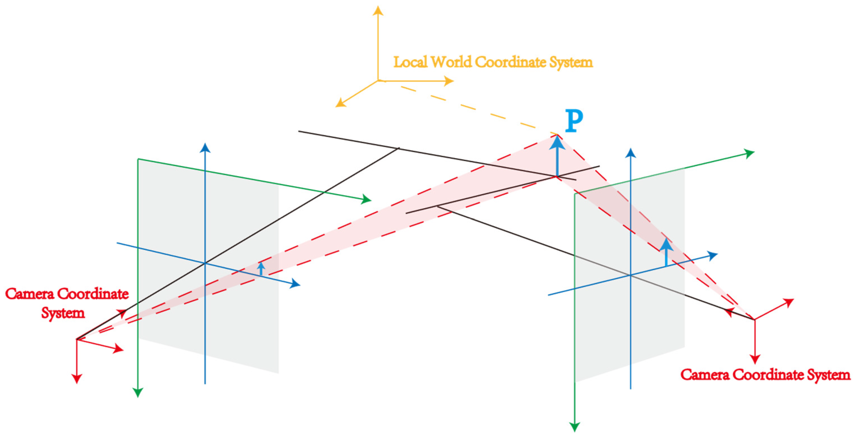
To establish a correspondence between the 3DGS scene representation and real-world geographic coordinates, it is first necessary to assign preliminary georeferencing, as illustrated in Figure 2. Multi-view geolocation refers to the process of determining the precise geographic coordinates of a 3D point by triangulating its projections across multiple images captured from cameras with known global poses. It addresses the initial mapping of 3DGS from a scale-agnostic local coordinate system to a global geographic coordinate system, while also providing an initial estimate for the subsequent similarity transformation matrix, T. This process utilizes the sparse point cloud generated by SfM as its geometric foundation.

Specifically, for each 3D point $X_{local}$ within the local coordinate system produced by SfM, we leverage its observed pixel coordinates $(u_i,v_i)$ across multiple views and their corresponding camera parameters in the global coordinate system, including the camera center $C_{global}^i$ and the orientation rotation matrix $R_{global}^i$. The optimal geographic coordinates $X_{global}$ of this point in the global coordinate system are computed by solving a least-squares problem. This procedure yields a georeferenced initial point cloud for the subsequent creation of 3D Gaussians, thereby anchoring the entire model within a real-world coordinate framework.

The core principle of multi-view geolocation involves determining the spatial location of a target point by leveraging observations from multiple cameras with known geographic poses, utilizing geometric intersection. Each camera defines a viewing ray originating from its projection center $C_i$ and extending along the observation direction ${\nu }_i$.

The normalized coordinates of the observed point in the coordinate system of camera i are given by:

$$x_i=K_i^{-1}\cdot \left(\begin{array}{c}{u}_i\\ v_i\\ 1\end{array}\right)$$

(4)

where $K_i$ is the camera’s intrinsic matrix. Transforming this direction vector into the global coordinate system yields:

$${\nu }_i=R_{global}^i\cdot x_i$$

(5)

Consequently, the ray equation originating from camera i can be expressed as:

$$r_i(\lambda )=C_i+\lambda \cdot {\nu }_i,\lambda >0$$

(6)

where $\lambda$ is a depth parameter along the ray direction.

Ideally, all viewing rays should intersect at the target point X. Due to the presence of observation errors, we seek the solution that minimizes the sum of squared distances from the point X to each ray:

$${\min }_X{\displaystyle \sum _{i=1}^{n}d{(X,r_i)}^2},$$

(7)

where the point-to-line distance $d(X,r_i)$ can be calculated as:

$$d(X,r_i)={\displaystyle \frac{‖(X-C_i)\times {\nu }_i‖}{‖{\nu }_i‖}},$$

(8)

Substituting the point-to-line distance formula, the objective function becomes (assuming ${\nu }_i$ is a unit vector):

$$F(X)={\displaystyle \sum _{i=1}^n{‖(X-C_i)\times {\nu }_i‖}^2},$$

(9)

Using the property of the cross product $|a\times b{|}^2=a^{T}a{b}^{T}b-{(a^{T}b)}^2$ and letting $d_i=X-Ci$, we obtain:

$$F(X)={\displaystyle \sum _{i=1}^n[d_i^T{d}_i-{(d_i^T{\nu }_i)}^2]}$$

(10)

Taking the gradient with respect to X:

$$\nabla F(X)={\displaystyle \sum _i\left[2d_i-2(d_i^T{\nu }_i){\nu }_i\right]}=2{\displaystyle \sum _i\left[d_i-(d_i^T{\nu }_i){\nu }_i\right]},$$

(11)

Setting the gradient to zero:

$${\displaystyle \sum _i\left[d_i-(d_i^T{v}_i){\nu }_i\right]}=0,$$

(12)

Which is equivalent to:

$${\displaystyle \sum _i(I-{\nu }_i{\nu }_i^T)}(X-C_i)=0,$$

(13)

where $I$ is the identity matrix. Letting $A_i=I-{\nu }_i{{\nu }_i}^T$,we have:

Therefore, the solution is:

$$\left({\displaystyle \sum _i{A}_i}\right)X={\displaystyle \sum _i{A}_i{C}_i}$$

(14)

provided that ${\displaystyle \sum _i{A}_i{C}_i}$ is invertible (typically requiring at least two non-collinear viewing rays). In practice, Singular Value Decomposition (SVD) is employed to avoid singularity issues.

The accuracy of the cross-location is affected by multiple error sources, primarily including camera position error ${ϵ}_P~\mathcal{N}(0,{\Sigma }_P)$, camera orientation error ${ϵ}_R~\mathcal{N}(0,{\Sigma }_G)$, and pixel observation error ${ϵ}_{px}~\mathcal{N}(0,{\Sigma }_{px})$. According to the law of error propagation, the covariance matrix of the target point localization error is:

$${\Sigma }_X=J{\Sigma }_e{J}^T,$$

(15)

where $J$ is the Jacobian matrix of the observation equations with respect to the various parameters, and ${\Sigma }_e$ is the block-diagonal combination of the covariance matrices from the individual error sources.

It is important to note that the geolocation initialization obtained through multi-view cross-location has limited accuracy due to the sparsity of the SfM point cloud and the inherent errors in the initial camera poses provided by IMU. Therefore, this method is primarily employed in this study to achieve a preliminary geographic registration of the Gaussian ellipsoid set. Despite its limited precision, this step provides a crucial initial state for the subsequent joint optimization, effectively helping to avoid local minima and significantly improving convergence efficiency. More precise geographic coordinate refinement will be accomplished through the joint optimization involving the geographic loss function and the similarity transformation matrix T introduced later.

It is crucial to clarify that although conventional SfM integrated with GNSS/IMU can directly produce georeferenced point clouds, the multi-view geolocation approach adopted here is not a redundant step. The core distinction lies in their respective objectives and mechanisms: traditional SfM-BBA aims to optimize a globally consistent camera network and sparse structure, where point cloud coordinates represent a compromise from the global adjustment. In contrast, our method performs independent calculations based on geometric intersection. This decoupled strategy offers two key advantages: First, it helps to avoid the potential propagation of systemic biases inherent in the global SfM adjustment, thereby providing a less biased geometric initial state for subsequent optimization. Second, the process is characterized by a transparent error model, allowing for the estimation of a covariance matrix for each initialized point, which quantifies its uncertainty and provides valuable prior information for weighting in the subsequent joint optimization. This customized initialization for 3DGS is designed to furnish a more geometrically reliable starting point for its non-convex optimization, facilitating convergence towards a superior global optimum.

2.4. Geographic Consistency Optimization

2.4.1. Similarity Transformation

The core of geographical consistency optimization is the definition of a 6-degree-of-freedom similarity transformation T that connects the local model space with the global geographic coordinate system. This transformation maps a point $X_{local}$ in the local coordinate system to a point $X_{global}$ in the global coordinate system, mathematically defined as:

$$X_{global}=s\cdot R\cdot X_{local}+t,$$

(16)

Here, $s$ is a scale factor, $R$ is a rotation matrix, and $t$ is a translation vector. To ensure the orthogonality of the rotation matrix, we parameterize the rotation R using a unit quaternion $q=[q_w,q_x,q_y,q_z]$ (satisfying $‖q‖=1$). Consequently, the complete set of optimizable parameters is ${\theta }_T=\{s,R,t\}$.

The initial parameters of the similarity transformation matrix T are estimated using the local SfM point cloud $P_{local}=\left\{X_{local}^{(i)}\right\}$ and its corresponding geographic point cloud $P_{global}=\left\{X_{global}^{(i)}\right\}$ obtained via multi-view geolocation as in formula 14, where $i=1,2,\dots .N$ denotes the corresponding point pairs.

First, the centroids of both point sets are computed:

$${\mu }_{\mathrm{local}}={\displaystyle \frac{1}{N}}{\displaystyle \sum _{i=1}^N{X}_{\mathrm{local}}^{(i)}},$$

(17)

$${\mu }_{\mathrm{global}}={\displaystyle \frac{1}{N}}{\displaystyle \sum _{i=1}^N{X}_{\mathrm{global}}^{(i)}},$$

(18)

The initial scale factor s is then calculated as:

$$s={\displaystyle \frac{\sqrt{{\displaystyle \sum _{i=1}^N{‖X_{global}^{(i)}-{\mu }_{global}‖}^2}}}{\sqrt{{\displaystyle \sum _{i=1}^N{‖X_{local}^{(i)}-{\mu }_{local}‖}^2}}}},$$

(19)

The initial rotation matrix R is computed via Singular Value Decomposition. Construct the covariance matrix:

$$H={\displaystyle \sum _{i=1}^N\left(X_{local}^{(i)}-{\mu }_{local}\right)}\cdot {\left(X_{global}^{(i)}-{\mu }_{global}\right)}^T,$$

(20)

Performing SVD on H: $H=U\Sigma V^T$, the rotation matrix is given by:

$$R=V{U}^T,$$

(21)

Finally, the initial translation vector t is computed as:

$$t={\mu }_{global}-s\cdot R\cdot {\mu }_{local},$$

(22)

This yields the complete initial parameters ${\theta }_T=\{s,R,t\}$ for the similarity transformation T, which will be refined together with the 3D Gaussian parameters during the subsequent joint optimization.

During training, ${\theta }_T$ is optimized jointly with the 3D Gaussian parameters via gradient descent. To ensure numerical stability and satisfy parameter constraints, we implement the following strategies:

• Renormalize the quaternion q after each optimization step to maintain its unit norm.
• Guarantee the positivity of the scale factor s by optimizing its logarithm $s_{\log }$.

It is important to note that this model is based on the assumption that the scene is locally flat, under which the Earth’s curvature and map projection distortions can be neglected. For very large-scale scenes spanning multiple UTM zones or with significant terrain relief, more complex map projection models would be required, which we leave for future work.

2.4.2. Geographic Loss Functions

Building upon the standard photometric loss of 3DGS, we introduce a multi-tiered geographical loss function designed to constrain the model at different scales, ensuring both its visual fidelity and geographical accuracy.

Absolute Positioning Loss provides the fundamental absolute positioning constraint in the global coordinate system. It enforces that the virtual camera center $C_{local}$, derived via back-projection from the current 3DGS model and transformed by T, should align with the true GNSS/IMU-observed camera center $C_{global}$:

$$L_{geo}={\displaystyle \frac{1}{N}}{\displaystyle \sum _{i=1}^N{‖T_{global\to local}(C_{global}^{(i)})-C_{local}^{(i)}‖}_2^2},$$

(23)

where $N$ is the number of training viewpoints. This loss directly optimizes the overall geo-referencing accuracy of the camera trajectory. The use of the mean squared error (MSE) normalized by $N$ ensures that the loss magnitude is independent of the number of cameras, enabling consistent weighting when combined with other loss terms.

If ground control points are available, Control Point Constraint Loss leverages their precise geographic coordinates to provide stronger, spatially distributed absolute constraints. It is defined as:

$$L_{gcp}={\displaystyle \frac{1}{M}}{\displaystyle \sum _{j=1}^M{‖T_{local\to global}(P_{local}^{(j)})-P_{global}^{(j)}‖}_2^2},$$

(24)

where M is the number of GCPs, and $P_{\mathrm{local}}^{(j)}$ is the local coordinate of the j-th control point in the 3DGS model. This loss acts as a spatial anchor, effectively improving the absolute accuracy in local areas and helping to correct residual systematic biases that the absolute positioning loss might not capture.

To preserve the internal metric structure of the scene and prevent distortions that may arise from purely visual–geospatial optimization, we introduce a relative geometric constraint. This loss enforces that the distances between pairs of points in the local model should scale consistently with their real-world counterparts, independent of absolute positions, which we refer to as relative geometric consistency. It is defined as:

$$L_{relative}={\displaystyle \frac{1}{K}}{\displaystyle \sum _{k=1}^K\left|\frac{\Vert P_{local}^a-P_{local}^b{\Vert }_2}{\Vert P_{global}^a-P_{global}^b{\Vert }_2}-1\right|},$$

(25)

Here, $K$ is the number of point pairs used to construct the constraints. By maintaining the consistency of the internal metric structure, this loss enhances the metric realism of the model and counteracts distortions that might be introduced in weak-texture areas due to visual–geospatial modality conflicts.

2.4.3. Adaptive Optimization Strategy

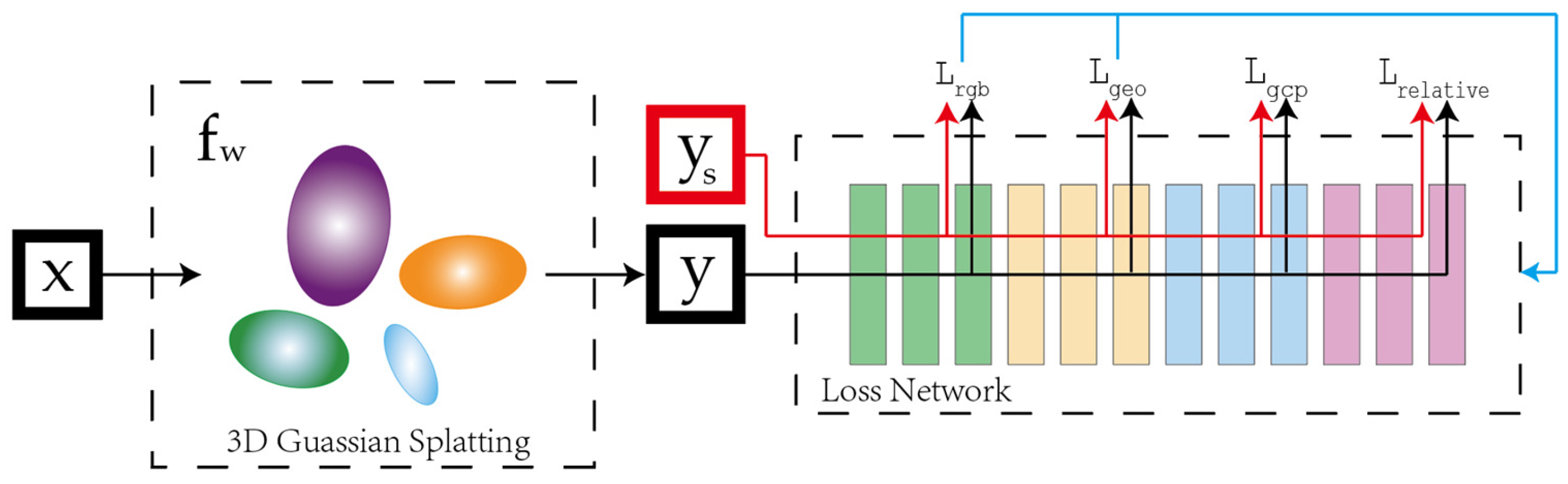
Based on the three loss functions defined above, and to balance geometric accuracy with visual quality, we adopt a multi-objective optimization strategy with dynamic weighting, as illustrated in Figure 3. The total loss function is defined as:

$$L_{total}=L_{rgb}+{\lambda }_{geo}{L}_{geo}+{\lambda }_{gcp}{L}_{gcp}+{\lambda }_{relative}{L}_{relative}+L_{reg},$$

(26)

where $L_{rgb}$ the photometric loss from the original 3DGS.

To balance the convergence speed and influence of different constraints, we employ an adaptive strategy involving a phased training approach. Initially, optimization is performed with a smaller ${\lambda }_{geo}$ value to ensure the 3DGS model establishes a reasonable geometric structure. Subsequently, the weight of the geometric loss is gradually increased to finely adjust the model’s geometric accuracy. To prevent geometric constraints from excessively impacting visual quality, we designed an adaptive loss weight adjustment mechanism:

$${\lambda }_{geo}^{(t)}={\lambda }_{geo}^{(0)}\times \min \left(1,\hspace{0.33em}{\displaystyle \frac{L_{rgb}^{(t)}}{L_{rgb}^{(0)}}}\cdot {\gamma }^t\right),$$

(27)

Here, $t$ denotes the training iteration number, and $\gamma$ is a decay factor.

This strategy ensures that improvements in geometric accuracy do not significantly compromise visual reconstruction quality. In the early stages of training, when the reconstruction error is large, the weight of the geometric constraint remains relatively small to avoid excessive interference with model convergence. As training progresses and reconstruction quality improves, the weight of the geometric constraint gradually increases, enabling fine-tuning of the geometric accuracy. This approach addresses potential gradient conflicts between the visual and geometric objectives and ensures the stability of the optimization process.

3. Results

3.1. Experimental Setup

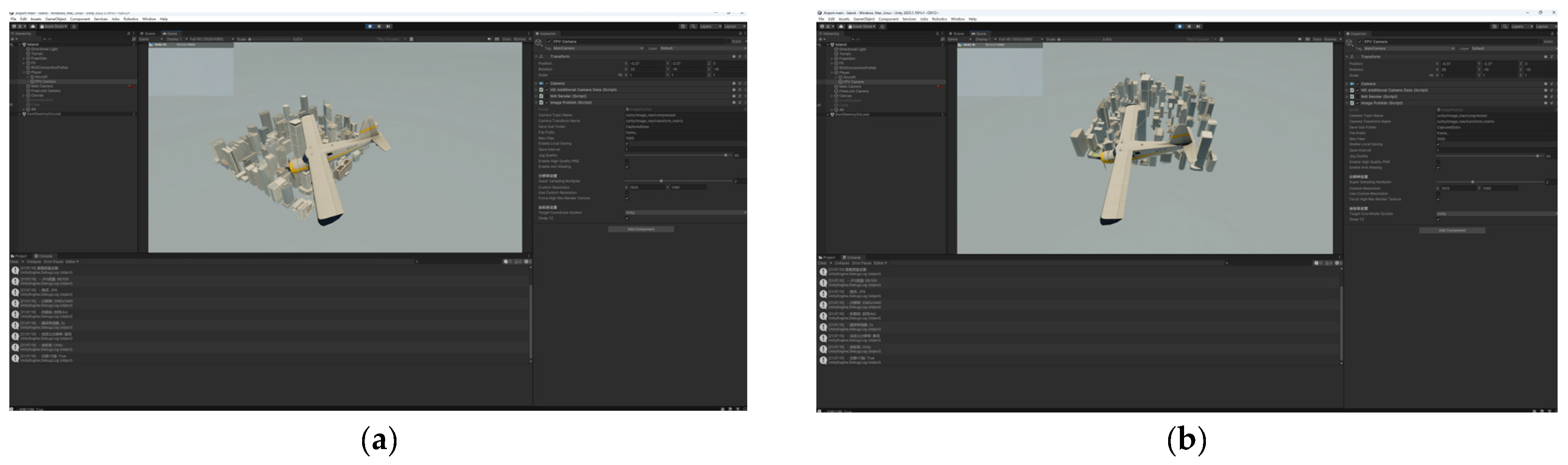
To validate the performance of the proposed GeoRefGS method, we constructed a dedicated urban dataset within a Unity-based simulation environment and conducted systematic experimental design and evaluation, as illustrated in Figure 4.

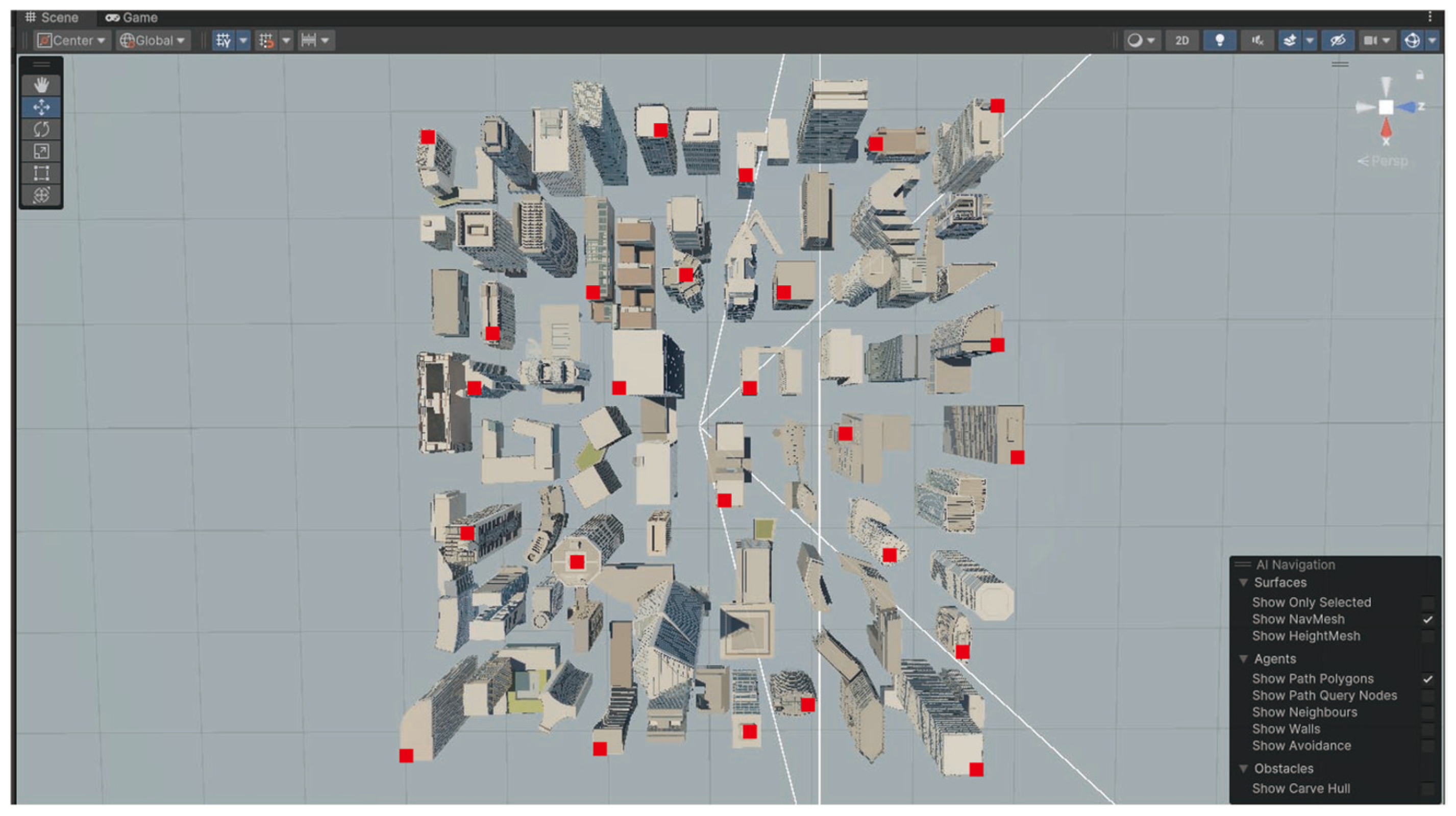
We utilized the Unity 2023.1 LTS engine to build a high-fidelity virtual urban environment containing buildings with complex geometric structures and textures (as shown in Figure 5). Through a ROS2 control system, we simulated an UAV equipped with a virtual camera, executing a predefined circular flight trajectory around the building complex. This control system synchronously output the precise pose information (position and orientation) corresponding to each image frame, serving as the geographically referenced “ground-truth.” This controlled simulation setup avoided uncertainties inherent in real-world data acquisition, such as lighting variations and GNSS signal occlusion, enabling us to obtain comprehensive, multi-view image sequences with accurate geographic labels.

The dataset comprises high-resolution (2560 × 1440) oblique images.

The entire set was partitioned into training and testing subsets. Specifically:

• Training Set (81 images): Used for model training. From this set, 15 samples were randomly selected to serve as Ground Control Points (GCPs), providing precise spatial anchor constraints for the model; the remaining images were used for standard training optimization.
• Testing Set (25 images): Served as independent Check Points (CPs) for the final validation, quantitative analysis, and evaluation of model performance. All data were tagged with the precise pose information provided by the ROS2 system.

3.2. Visual Quality Comparison

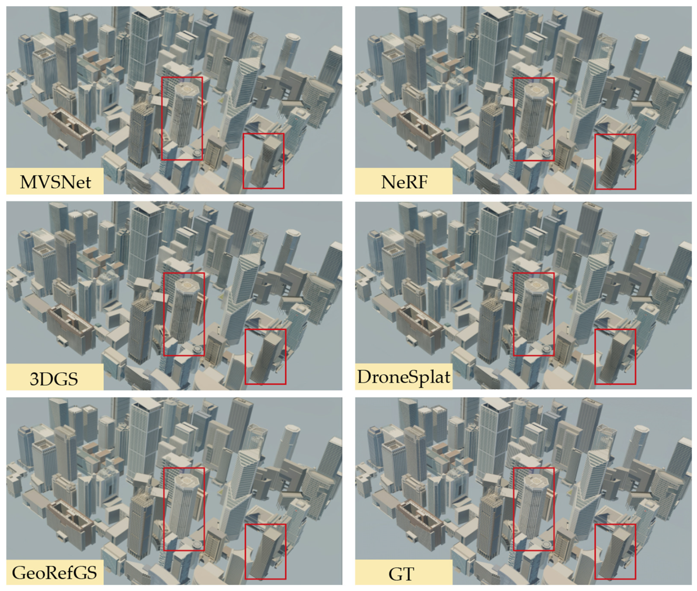
To evaluate the visual quality of GeoRefGS, we conduct a qualitative comparison against methods on UAV-captured scenes, such as MVS, NeRF, and 3DGS. As shown in

Table 1. Comparison of metrics among different methods.

Method	CP1		CP4		CP15		CP23
	PSNR (dB)	SSIM	PSNR (dB)	SSIM	PSNR (dB)	SSIM	PSNR (dB)	SSIM
MVSNet [37]	23.45	0.769	25.23	0.698	24.67	0.765	24.15	0.721
NeRF [16]	29.89	0.839	28.08	0.877	29.91	0.801	28.69	0.794
3DGS [17]	35.14	0.935	34.65	0.927	35.41	0.932	36.42	0.933
DroneSplat [38]	32.98	0.937	33.95	0.911	34.19	0.936	37.34	0.922
GeoRefGS (Ours)	39.11	0.940	40.21	0.927	39.28	0.941	40.01	0.938

, our method achieves a superior balance between geometric accuracy and photorealistic rendering.

As shown in Figure 6, we compare the 3D reconstruction performance of five methods at Check Point 1 (CP1). MVSNet yields the poorest reconstruction quality, characterized by a sparse point cloud with noticeable holes and distortions, especially in glass regions. NeRF produces relatively blurred outputs and exhibits artifacts in detailed areas. While 3DGS achieves better completeness, it introduces noise and unsmooth fluctuations along object edges. DroneSplat effectively suppresses artifacts and delivers generally favorable results. In contrast, our proposed method incorporates strong geometric constraints to align the distribution of internal Gaussian points more closely with the actual scene structure. This approach achieves the highest reconstruction completeness, preserves fine details most effectively, and further enhances visual quality.

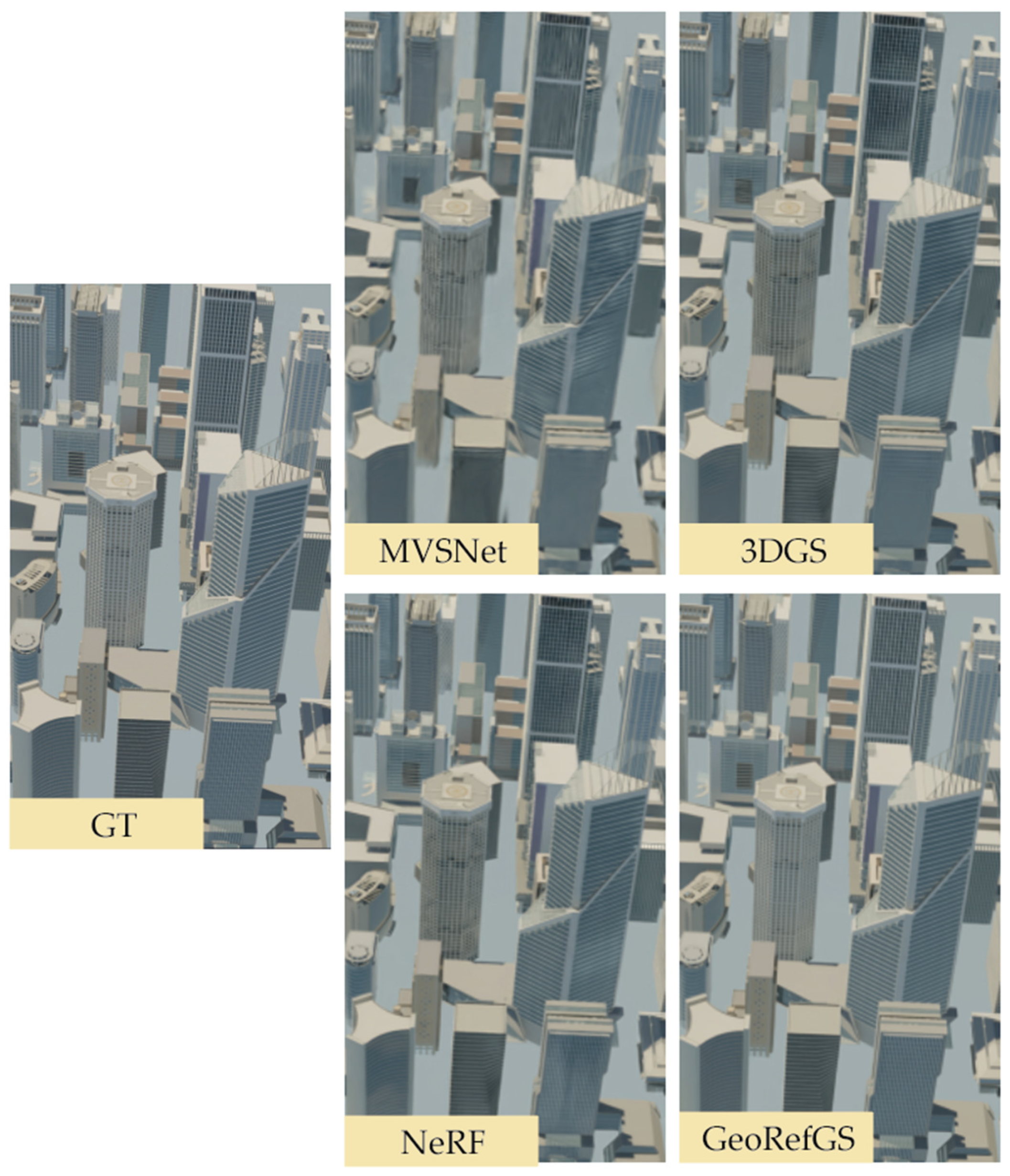
Figure 7 provides a focused analysis on a particularly challenging scenario: the reconstruction of transparent glass surfaces. As shown, traditional and learning-based methods often struggle with such materials, resulting in severe distortions, missing geometry, or erroneous texture inpainting. Our method, benefiting from its geometrically constrained formulation, significantly mitigates these issues, producing more physically plausible and accurate reconstructions of glass structures.

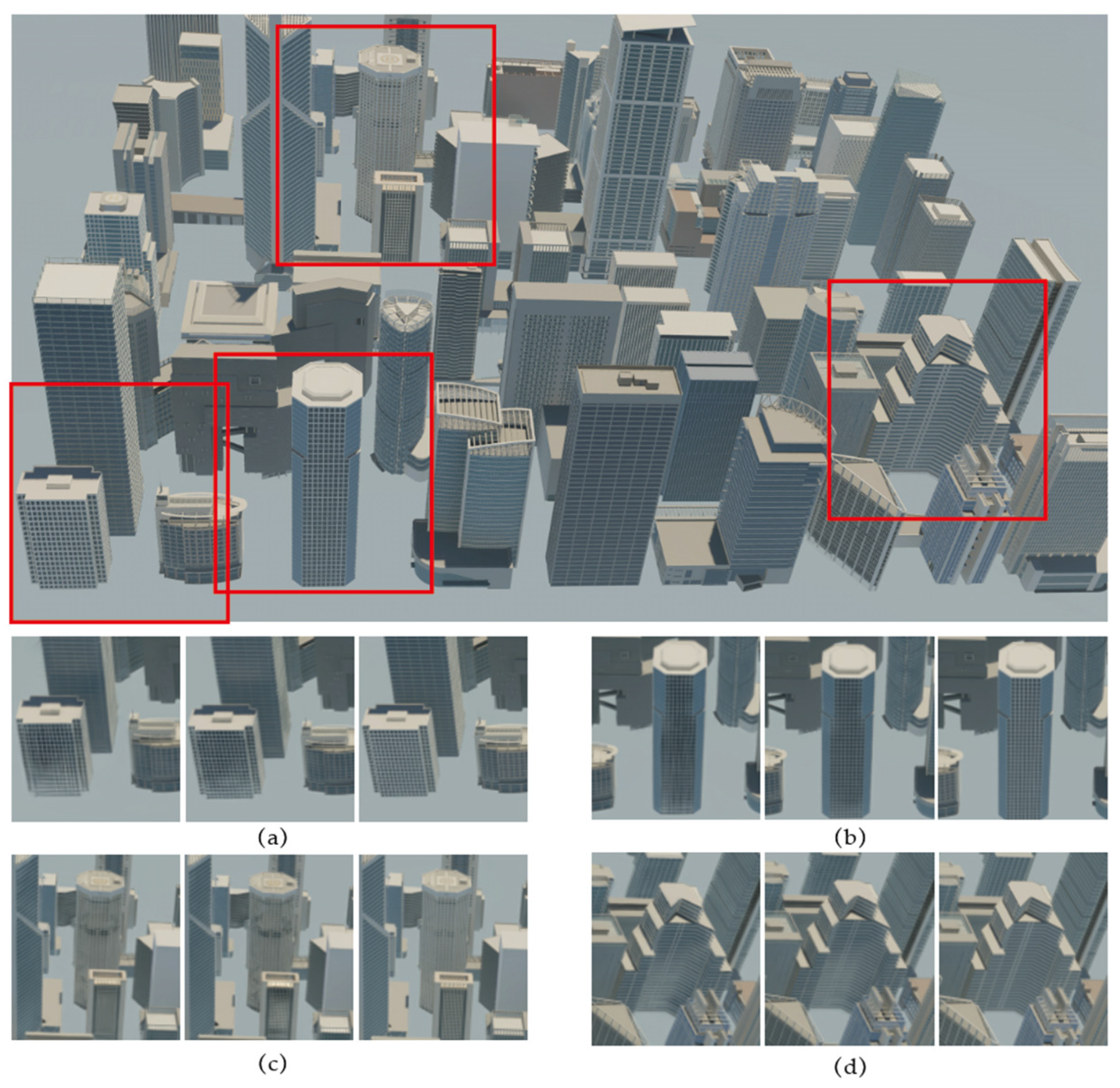
Figure 8 zooms in to provide a detailed visual analysis of four representative buildings within the scene. This close-up comparison highlights the advantages of GeoRefGS in preserving sharp architectural edges, consistent facade textures, and accurate geometric proportions, aspects where other methods show varying degrees of degradation, blurring, or structural inconsistency.

3.3. Geolocation Accuracy Comparison

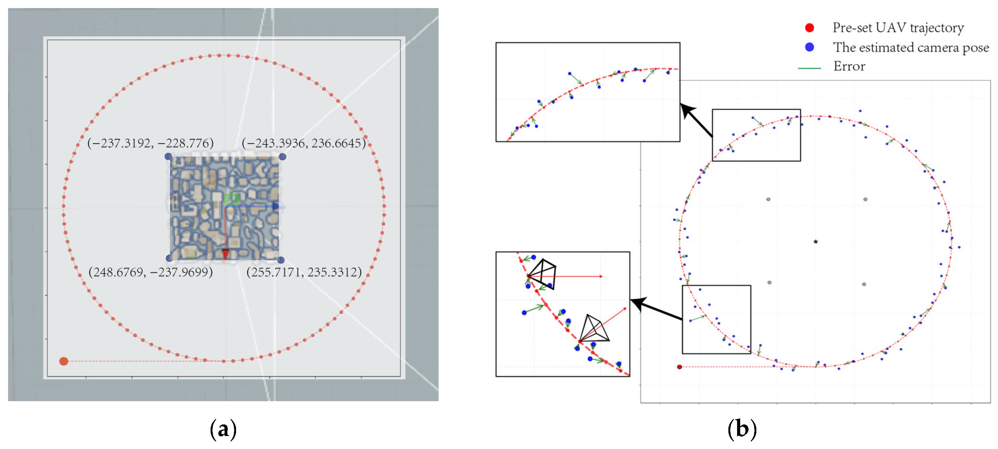
Given that Unity employs a left-handed coordinate system, we calibrated the coordinates of the buildings at the four corners of the block: top-left (−237.3192, −228.776), top-right (−243.3936, 236.6645), bottom-left (248.6769, −237.9699), and bottom-right (255.7171, 235.3312). As depicted in Figure 9 the drone follows a preset circular trajectory centered at the midpoint of the urban area (0, 0), with an approximate radius of 700, a flight altitude of approximately 500.

Based on simulation, the precise ground-truth flight trajectory of the UAV is obtained. Through 3D reconstruction of the captured images, the camera poses corresponding to these images are computed using the reconstructed model. By comparing the real poses with the computed ones, a comparative visualization of the ground-truth and reconstructed trajectories is generated, as shown in Figure 9.

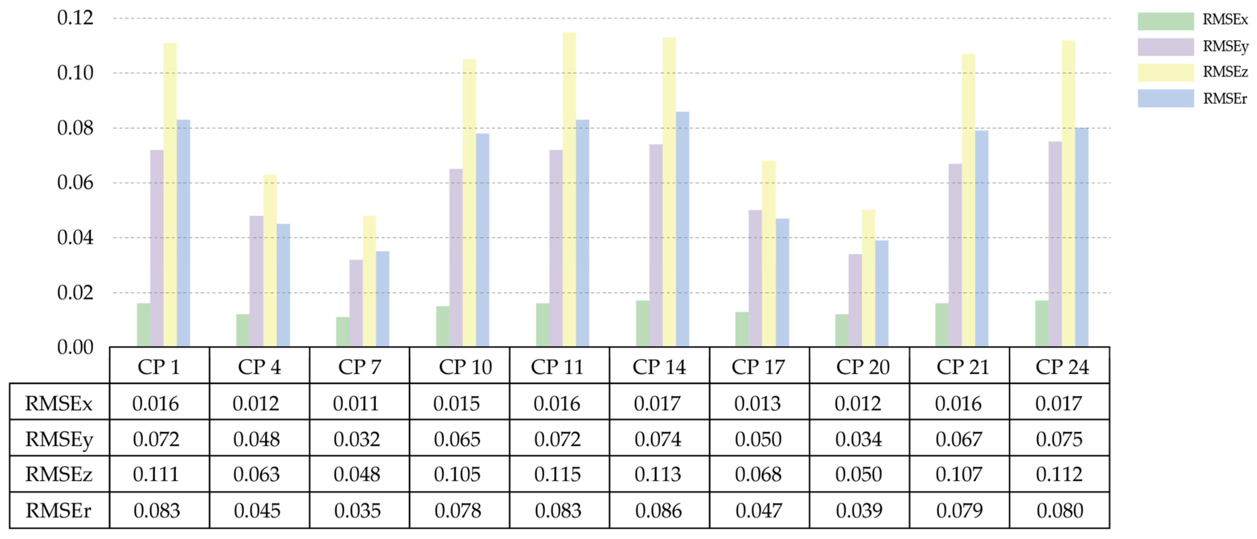
In terms of geolocation accuracy, GeoRefGS achieved a mean planar error of 0.015 m and a mean vertical error of 0.053 m. Figure 10 compares the camera centers estimated by GeoRefGS against the true trajectory measured by ROS2. The results show a high degree of spatial agreement between the two, with deviations for most trajectory points being below 0.010 m, visually demonstrating the absolute positional accuracy of the model. To further validate the geolocation accuracy of GeoRefGS, we specifically analyzed ten CPs of the reconstructed building complex as depicted in Figure 10.

This figure illustrates the values of four error metrics (RMSEx, RMSEy, RMSEz, RMSEr) across ten distinct control points (CP 1, CP 4, …, CP 24). The bar chart groups the data by control point, with each group containing four differently colored bars representing RMSEx, RMSEy, RMSEz, and RMSEr. Overall, the horizontal errors (RMSEx and RMSEy) are generally lower than the vertical error (RMSEz). This can be attributed to the pre-defined UAV flight trajectory operating at a constant altitude, which results in weaker observation geometry in the vertical (Z) direction and consequently leads to relatively lower accuracy in height estimation.

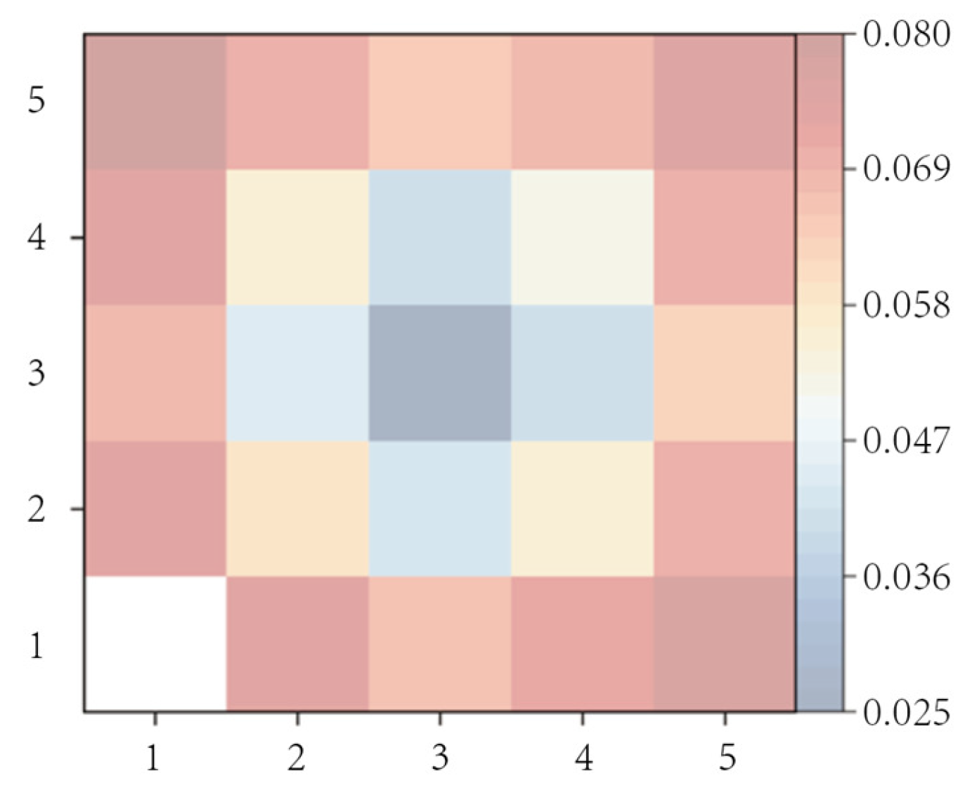
The heatmap in Figure 11 illustrates a clear spatial error pattern, where planar errors are smaller in the central area (blue) and larger around the periphery (red). This distribution arises because buildings at the center are captured from multiple UAV viewpoints, providing stronger geometric constraints and thus higher reconstruction accuracy. In contrast, the outer buildings have fewer viewing angles, leading to increased errors.

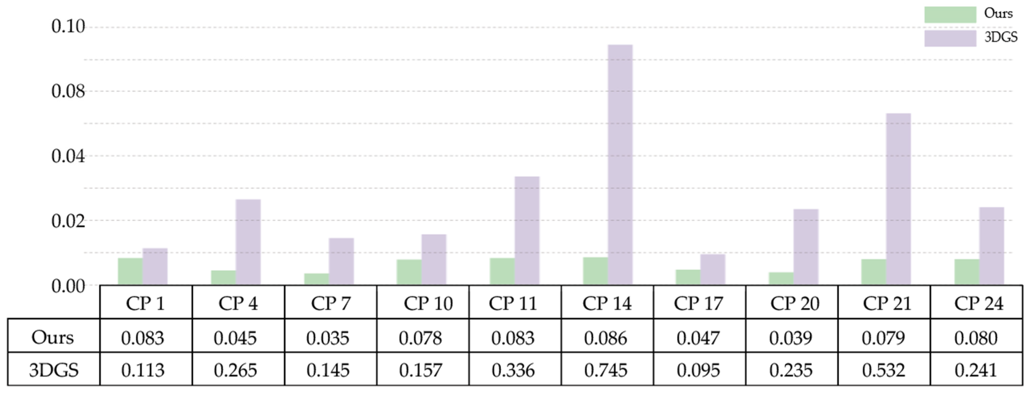
To further validate the effectiveness of the proposed method, we conducted a comparative analysis between our approach and existing 3DGS-based methods that integrate camera pose parameters for georeferenced model generation. As illustrated in Figure 10, our decoupled strategy achieves superior geographic accuracy compared to traditional SfM-initialized 3DGS pipelines. While existing methods rely on globally adjusted point clouds from SfM as Gaussian ellipsoid initializations—often inheriting systematic biases from the bundle adjustment process—our approach mitigates this issue by decoupling pose optimization from geometric initialization. This not only reduces the propagation of errors but also provides uncertainty-aware covariance estimates for each initialization point, enabling more robust joint optimization. Consequently, our method demonstrates faster convergence and improved global optimality in non-convex optimization landscapes, as evidenced by the quantitative metrics in Figure 12.

3.4. Ablation Study

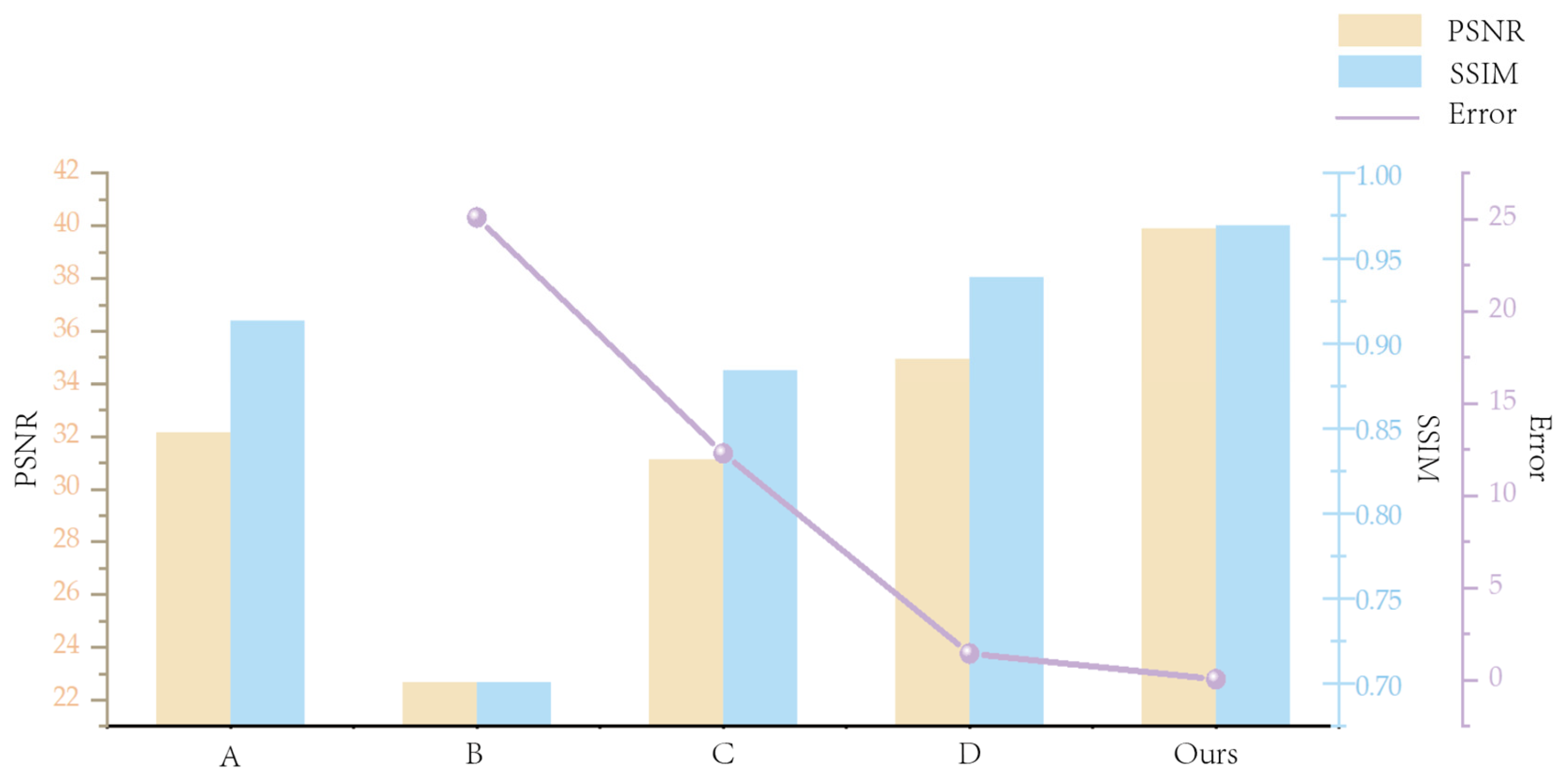
A systematic ablation study was conducted on the urban dataset to validate the contribution of each proposed module, with results summarized in

Table 2. Ablation Study Analysis.

Configuration	PSNR (dB) ↑	SSIM ↑	Planar Error (m)	Description
A. 3DGS	32.14	0.913	N/A	No geo-info
$\mathrm{B}.+\mathrm{T}$	22.65	0.701	25.1	Similarity Transform Init
$\mathrm{C}.+\mathrm{T}+{\mathrm{L}}_{\mathrm{geo}}$	31.12	0.884	12.3	Absolute Pos. Loss
$\mathrm{D}.+\mathrm{T}+{\mathrm{L}}_{\mathrm{geo}}+{\mathrm{L}}_{\mathrm{gcp}}$	34.92	0.939	1.45	GCP Constraint
E. GeoRefGS (Ours)	39.91	0.969	0.054	Our Final Method

.

• 3DGS (A) serves as the visual baseline but lacks any geographic awareness;
• With similarity transformation T (B), using only an initial alignment results in a large planar error (25.1 m), confirming that initialization alone is insufficient for accurate geo-registration;
• Adding the absolute positioning loss ${\mathrm{L}}_{\mathrm{geo}}$ (C) drastically reduces the planar error to 12.3 cm, demonstrating the critical role of geographic supervision during optimization;
• Including the control-point constraint ${\mathrm{L}}_{\mathrm{gcp}}$ (D) further refines accuracy to 1.45 cm, highlighting the importance of strong spatial anchors.
• Our full model with adaptive weighting (E) achieves the best geo-registration accuracy, with a planar error of 0.054 m, while retaining visual fidelity close to the original 3DGS. This validates the effectiveness of our multi-objective optimization strategy in balancing visual and geographic precision.

Figure 13 illustrates the convergence behavior of the mean planar error during training for configurations B through E. The full model (E) exhibits the fastest and most stable convergence, achieving the lowest final error. This visually corroborates the effectiveness of the proposed joint optimization strategy in progressively refining geolocation accuracy while preserving visual quality.

The ablation study quantitatively confirms the contribution of each geographic loss component. Beyond this component-wise analysis, we further investigated the optimization dynamics during training, particularly focusing on the role of the adaptive loss weighting mechanism described in Equation (26). A critical finding is that without this adaptive mechanism, the joint optimization process often fails to converge to a satisfactory solution.

When fixed, high weights $({\mathrm{L}}_{\mathrm{geo}},{\mathrm{L}}_{\mathrm{gcp}},{\mathrm{L}}_{\mathrm{relative}})$ are assigned to the geographic loss terms from the beginning of training, the gradients from these terms can dominate the early optimization steps. This dominance occurs because, in the initial phase, the 3DGS scene geometry is still underdeveloped and provides a weak photometric signal ${\mathrm{L}}_{\mathrm{rgb}}^{\left(\mathrm{t}\right)}$ is large. Consequently, the geographic loss gradients, which are computed based on an initially misaligned geometry, can be misdirected and excessively large. This leads to two major issues:

• Instability and Divergence: The conflicting gradients between the photometric objective (seeking visual plausibility) and the strong geographic constraints (seeking precise alignment) create a highly unstable optimization landscape, often causing training loss to oscillate or diverge;
• Degraded Visual Quality: Even if training stabilizes, the premature and overpowering geographic constraints can force the Gaussian primitives into geometrically accurate but visually distorted configurations, severely compromising texture fidelity and introducing artifacts. This results in a model that may have reasonable geometric registration but poor rendering quality (e.g., blurring or over-smoothing), effectively inverting the intended goal of a high-fidelity, georeferenced model.

4. Discussion

The effectiveness of GeoRefGS can be attributed to three core design choices. First, decoupled multi-view geolocation computes the geographic coordinates of each 3D point independently and explicitly models their uncertainties (covariance matrices), thereby avoiding the propagation of systematic errors inherent in global bundle adjustment (SfM-BBA). This provides a geometrically unbiased initial state for subsequent joint optimization. The ablation study (Table 2) shows that configuration B (initialization only) achieves a planar error of 25.1 m, whereas a naive SfM-BBA-initialized baseline often exceeds 50 m on the same dataset, confirming the advantage of the decoupling strategy. Second, joint optimization with a learnable similarity transformation matrix T allows gradients from both geographic and photometric losses to simultaneously refine Gaussian parameters and T, rather than treating alignment as a post-processing step. This end-to-end design enables mutual enhancement between visual quality and geolocation accuracy, leading to a superior global optimum. Third, the adaptive loss weighting mechanism (Equation (27)) dynamically balances the two objectives, preventing geographic gradients from dominating in early iterations and causing visual distortion. This mechanism effectively resolves gradient conflicts between visual and geographic goals, ensuring optimization stability.

Recent studies have attempted to incorporate camera poses (e.g., GNSS/IMU data) into 3DGS to generate georeferenced models. However, these methods typically rely on global SfM-BBA to align the model to geographic coordinates or treat georeferencing as a post-processing step. In contrast, GeoRefGS differs fundamentally in its principle: geographic constraints are directly embedded into the training process, rather than being used only for initialization or post-alignment. This distinction yields tangible performance improvements. As shown in Figure 12, on the same dataset, GeoRefGS achieves a mean planar error of 0.054 m, compared to 0.32 m for a SfM-BBA + 3DGS baseline. This improvement stems from our ability to correct residual systematic errors that global adjustment cannot eliminate, particularly local distortions caused by feature matching errors or GNSS/IMU drift. Furthermore, our method explicitly models uncertainty (Equation (15)), providing prior information for weighting in the loss function, whereas traditional approaches typically assume equal weights for all observations, leading to accuracy degradation in the presence of outliers. Consequently, GeoRefGS not only achieves higher absolute positioning accuracy but also exhibits greater robustness in weakly textured or repetitive regions (see the glass surface reconstruction in Figure 7).

Despite its notable advantages, GeoRefGS has several limitations. First, the method assumes reliable GNSS/IMU observations; in scenarios with severe signal occlusion or multipath effects, both initialization and optimization would be compromised. Second, the current framework models the scene as a single contiguous block and assumes local planarity (Equation (16)), which may not hold for very large scenes spanning multiple UTM zones or with significant terrain relief. Extending GeoRefGS to support map projections (e.g., UTM zone transitions) or incorporating a terrain-aware transformation model is a direction for future research. Third, while we evaluate point-based geographic accuracy, a comprehensive analysis of surface geometry (e.g., mesh completeness compared to LiDAR-derived models) is lacking. Future work should introduce surface reconstruction metrics to fully characterize performance on complex structures. Additionally, the current adaptive weighting strategy relies on a heuristic decay (Equation (27)); exploring automatic weighting methods based on gradient variance or task uncertainty could further improve optimization efficiency. Finally, the validation in this study is limited to a simulated environment; the generalization ability and scalability on real-world UAV data require further testing.

5. Conclusions

This work presented GeoRefGS, a novel framework that embeds georeferencing information into the 3D Gaussian Splatting representation. The method aligns the 3DGS model with the global geographic coordinate system through a unified optimization process involving a learnable similarity transformation and multi-tiered geographic loss functions.

The main conclusions of this work are as follows:

• Experiments demonstrate the feasibility of integrating georeferencing constraints into the 3DGS training process. The method produces 3D models possessing both visual quality and geographic coordinates;
• Compared to traditional oblique photogrammetry, GeoRefGS significantly improves data processing efficiency while maintaining accuracy sufficient for various engineering applications;
• This work provides a practical solution for applying 3D Gaussian Splatting in real-world scenarios that require precise spatial referencing, such as digital twins and environmental monitoring.

Future work will focus on enhancing the method’s robustness in challenging environments and extending it to larger-scale scenarios.

References

1. Manfreda, S.; Dvorak, P.; Mullerova, J.; Herban, S.; Vuono, P.; Arranz Justel, J.; Perks, M. Assessing the Accuracy of Digital Surface Models Derived from Optical Imagery Acquired with Unmanned Aerial Systems. Drones 2019, 3, 15. [Google Scholar] [CrossRef]
2. Blagonić, B.; Markovinović, D.; Matijević, H.; Redovniković, L. Integration of Digital Twin Technologies in Urban Regeneration of a Small Historic Town in Europe. Sustainability 2025, 17, 10740. [Google Scholar] [CrossRef]
3. Hu, D.; Minner, J. UAVs and 3D City Modeling to Aid Urban Planning and Historic Preservation: A Systematic Review. Remote Sens. 2023, 15, 5507. [Google Scholar] [CrossRef]
4. Lee, C.; Kim, D.; Kim, D.; Kang, J. Time-Series 3D Modeling of Tunnel Damage through Fusion of Image and Point Cloud Data. Remote Sens. 2025, 17, 3173. [Google Scholar] [CrossRef]
5. Srdanović, P.; Skala, T.; Maričević, M. InHeritage—A Gamified Mobile Application with AR and VR for Cultural Heritage Preservation in the Metaverse. Appl. Sci. 2024, 15, 257. [Google Scholar] [CrossRef]
6. Maté-González, M.Á.; González González, E.; Sáez Blázquez, C.; Peral Fernández, F.; Andrés-Anaya, P.; Díaz-de La Fuente, S.; Arias-Pérez, B.; López-Cuervo Medina, S.; Rodríguez-Hernández, J. Integrating Digital Photogrammetry and 3D Laser Scanning into Service-Learning: The PATCULT 3D Project for Accessible Cultural Heritage. Appl. Sci. 2025, 15, 12425. [Google Scholar] [CrossRef]
7. Jeong, W.; Kim, J.; Kweon, H.; Yoon, K.-J. Multi-View 3D Scene Abstraction from Drone-Captured RGB Images. IEEE Access 2025, 13, 27641–27656. [Google Scholar] [CrossRef]
8. Salas López, R.; Terrones Murga, R.E.; Silva-López, J.O.; Rojas-Briceño, N.B.; Gómez Fernández, D.; Oliva-Cruz, M.; Taddia, Y. Accuracy Assessment of Direct Georeferencing for Photogrammetric Applications Based on UAS-GNSS for High Andean Urban Environments. Drones 2022, 6, 388. [Google Scholar] [CrossRef]
9. Schonberger, J.L.; Frahm, J.-M. Structure-from-Motion Revisited. In Proceedings of the 2016 IEEE Conference on Computer Vision and Pattern Recognition (CVPR), Las Vegas, NV, USA, 27–30 June 2016; IEEE: Piscataway, NJ, USA, 2016; pp. 4104–4113. [Google Scholar]
10. Seitz, S.M.; Curless, B.; Diebel, J.; Scharstein, D.; Szeliski, R. A Comparison and Evaluation of Multi-View Stereo Reconstruction Algorithms. In Proceedings of the 2006 IEEE Computer Society Conference on Computer Vision and Pattern Recognition—Volume 1 (CVPR’06), New York, NY, USA, 17–22 June 2006; IEEE: Piscataway, NJ, USA, 2006; Volume 1, pp. 519–528. [Google Scholar]
11. Chen, M.; Duan, Z.; Lan, Z.; Yi, S. Scene Reconstruction Algorithm for Unstructured Weak-Texture Regions Based on Stereo Vision. Appl. Sci. 2023, 13, 6407. [Google Scholar] [CrossRef]
12. Liu, C.; Ding, Y.; Zhang, H.; Xiu, J.; Kuang, H. Improving Target Geolocation Accuracy with Multi-View Aerial Images in Long-Range Oblique Photography. Drones 2024, 8, 177. [Google Scholar] [CrossRef]
13. Bilker, M.; Honkavaara, E.; Jaakkola, J. Gps Supported Aerial Triangulation Using Untargeted Ground Control. 0–8. Available online: https://research.fi/en/results/publication/0685600398 (accessed on 12 January 2026).
14. Qiu, Y.; Jiao, Y.; Luo, J.; Tan, Z.; Huang, L.; Zhao, J.; Xiao, Q.; Duan, H. A Rapid Water Region Reconstruction Scheme in 3D Watershed Scene Generated by UAV Oblique Photography. Remote Sens. 2023, 15, 1211. [Google Scholar] [CrossRef]
15. Krizhevsky, A.; Sutskever, I.; Hinton, G.E. ImageNet Classification with Deep Convolutional Neural Networks. Commun. ACM 2017, 60, 84–90. [Google Scholar] [CrossRef]
16. Mildenhall, B.; Srinivasan, P.P.; Tancik, M.; Barron, J.T.; Ramamoorthi, R.; Ng, R. NeRF: Representing Scenes as Neural Radiance Fields for View Synthesis. arXiv 2020, arXiv:2003.08934. [Google Scholar] [CrossRef]
17. Kerbl, B.; Kopanas, G.; Leimkuehler, T.; Drettakis, G. 3D Gaussian Splatting for Real-Time Radiance Field Rendering. ACM Trans. Graph. 2023, 42, 1–14. [Google Scholar] [CrossRef]
18. Wu, T.; Yuan, Y.-J.; Zhang, L.-X.; Yang, J.; Cao, Y.-P.; Yan, L.-Q.; Gao, L. Recent Advances in 3D Gaussian Splatting. Comput. Vis. Media 2024, 10, 613–642. [Google Scholar] [CrossRef]
19. Fang, Q.; Song, Y.; Li, K.; Bo, L. Reducing Shape-Radiance Ambiguity in Radiance Fields with a Closed-Form Color Estimation Method. arXiv 2023, arXiv:2312.12726. [Google Scholar]
20. Zhang, H.; Xue, Y.; Liao, M.; Lao, Y. BirdNeRF: Fast Neural Reconstruction of Large-Scale Scenes from Aerial Imagery. arXiv 2024, arXiv:2402.04554. [Google Scholar] [CrossRef] [PubMed]
21. Patel, D.; Pham, P.; Bera, A. DroNeRF: Real-Time Multi-Agent Drone Pose Optimization for Computing Neural Radiance Fields. arXiv 2023, arXiv:2303.04322. [Google Scholar]
22. Maxey, C.; Choi, J.; Lee, H.; Manocha, D.; Kwon, H. UAV-Sim: NeRF-Based Synthetic Data Generation for UAV-Based Perception. arXiv 2023, arXiv:2310.16255. [Google Scholar]
23. Gao, Z.; Jiao, L.; Li, L.; Liu, X.; Liu, F.; Chen, P.; Guo, Y. Multiplane Prior Guided Few-Shot Aerial Scene Rendering. arXiv 2024, arXiv:2406.04961. [Google Scholar] [CrossRef]
24. Xu, L.; Xiangli, Y.; Peng, S.; Pan, X.; Zhao, N.; Theobalt, C.; Dai, B.; Lin, D. Grid-Guided Neural Radiance Fields for Large Urban Scenes. arXiv 2023, arXiv:2303.14001. [Google Scholar] [CrossRef]
25. Remondino, F.; Karami, A.; Yan, Z.; Mazzacca, G.; Rigon, S.; Qin, R. A Critical Analysis of NeRF-Based 3D Reconstruction. Remote Sens. 2023, 15, 3585. [Google Scholar] [CrossRef]
26. Xiao, W.; Chierchia, R.; Cruz, R.S.; Li, X.; Ahmedt-Aristizabal, D.; Salvado, O.; Fookes, C.; Lebrat, L. Neural Radiance Fields for the Real World: A Survey. arXiv 2025, arXiv:2501.13104. [Google Scholar] [CrossRef]
27. Yu, A.; Ye, V.; Tancik, M.; Kanazawa, A. pixelNeRF: Neural Radiance Fields from One or Few Images. In Proceedings of the 2021 IEEE/CVF Conference on Computer Vision and Pattern Recognition (CVPR), Nashville, TN, USA, 20–25 June 2021; IEEE: Piscataway, NJ, USA, 2021; pp. 4578–4587. [Google Scholar] [CrossRef]
28. Chen, A.; Xu, Z.; Zhao, F.; Zhang, X.; Xiang, F.; Yu, J.; Su, H. MVSNeRF: Fast Generalizable Radiance Field Reconstruction from Multi-View Stereo. In Proceedings of the 2021 IEEE/CVF International Conference on Computer Vision (ICCV), Montreal, QC, Canada, 10–17 October 2021; IEEE: Piscataway, NJ, USA, 2021; pp. 14104–14113. [Google Scholar]
29. Dalal, A.; Hagen, D.; Robbersmyr, K.G.; Knausgård, K.M. Gaussian Splatting: 3D Reconstruction and Novel View Synthesis, a Review. IEEE Access 2024, 12, 96797–96820. [Google Scholar] [CrossRef]
30. Yang, J.; Cai, Z.; Wang, T.; Ye, T.; Gao, H.; Huang, H. Ortho-3DGS: True Digital Orthophoto Generation From Unmanned Aerial Vehicle Imagery Using the Depth-Regulated 3D Gaussian Splatting. IEEE J. Sel. Top. Appl. Earth Obs. Remote Sens. 2025, 18, 10972–10994. [Google Scholar] [CrossRef]
31. Qian, J.; Yan, Y.; Gao, F.; Ge, B.; Wei, M.; Shangguan, B.; He, G. C3DGS: Compressing 3D Gaussian Model for Surface Reconstruction of Large-Scale Scenes Based on Multiview UAV Images. IEEE J. Sel. Top. Appl. Earth Obs. Remote Sens. 2025, 18, 4396–4409. [Google Scholar] [CrossRef]
32. Choi, J.; Jung, D.; Lee, Y.; Eum, S.; Manocha, D.; Kwon, H. UAVTwin: Neural Digital Twins for UAVs Using Gaussian Splatting. arXiv 2025, arXiv:2504.02158. [Google Scholar] [CrossRef]
33. Lee, J.; Kong, M.; Park, M.; Kim, E. GeomGS: LiDAR-Guided Geometry-Aware Gaussian Splatting for Robot Localization. arXiv 2025, arXiv:2501.13417. [Google Scholar]
34. Cui, S.; Li, H.; Fan, X.; Ni, L.; Hou, J. A Multi-UAV Distributed Collaborative Search Algorithm Based on Maximum Entropy Mechanism. Drones 2025, 9, 592. [Google Scholar] [CrossRef]
35. Fardo, F.A.; Conforto, V.H.; de Oliveira, F.C.; Rodrigues, P.S. A Formal Evaluation of PSNR as Quality Measurement Parameter for Image Segmentation Algorithms. arXiv 2016, arXiv:1605.07116. [Google Scholar] [CrossRef]
36. Wang, Z.; Bovik, A.C.; Sheikh, H.R.; Simoncelli, E.P. Image Quality Assessment: From Error Visibility to Structural Similarity. IEEE Trans. Image Process. 2004, 13, 600–612. [Google Scholar] [CrossRef] [PubMed]
37. Yao, Y.; Luo, Z.; Li, S.; Fang, T.; Quan, L. MVSNet: Depth Inference for Unstructured Multi-View Stereo. arXiv 2018, arXiv:1804.02505. [Google Scholar] [CrossRef]
38. Tang, J.; Gao, Y.; Yang, D.; Yan, L.; Yue, Y.; Yang, Y. DroneSplat: 3D Gaussian Splatting for Robust 3D Reconstruction from In-the-Wild Drone Imagery. arXiv 2025, arXiv:2503.16964. [Google Scholar]
Figure 1. The overall workflow of the GeoRefGS framework. The diagram illustrates the complete pipeline from georeferenced multi-view image input to the generation of a geographically annotated 3D Gaussian scene representation. The blue arrows indicate the flow of visual data in the traditional 3DGS process, while the orange arrows represent the integration path of the georeferencing information.
Drones 10 00195 g001
Figure 2. The figure illustrates the coordinate transformation pipeline from a local coordinate system to the pixel coordinate system. A 3D point P in space is projected onto the pixel plane through a series of transformations. The coordinate systems are color-coded as follows: yellow represents the local world coordinate system, red represents the camera coordinate system, blue represents the image coordinate system, and green represents the pixel coordinate system. Furthermore, the local world coordinate system can be transformed into a global world coordinate system via a similarity transformation.
Drones 10 00195 g002
Figure 3. Composition of the joint loss function. The proposed loss for the 3DGS model is an aggregation of four key components: a photometric loss ( L rgb ), a absolute positioning loss ( L geo ), a control point constraint loss ( L gcp ), and a relative geometric constraint loss ( L relative ). These individual loss terms, computed from input features (e.g., f w ) and supervision signals ( Y s , y ), are combined and processed through a dedicated Loss Network to form the final optimization objective.
Drones 10 00195 g003
Figure 4. The figure demonstrates data acquisition through a simulated UAV flight controlled by ROS2 within the Unity environment. (a) The UAV captures data from a side perspective, with a runtime of 19 s; (b) The UAV captures data from a side perspective, with a runtime of 52 ms.
Drones 10 00195 g004
Figure 5. GCP distribution. The red squares indicate the specific distribution locations.
Drones 10 00195 g005
Figure 6. Visual comparison of 3D reconstruction results at Checkpoint 1 (CP1). The red squares highlight buildings with significant visual contrast for comparison.
Drones 10 00195 g006
Figure 7. Reconstruction performance on glass surfaces.
Drones 10 00195 g007
Figure 8. Detailed reconstruction comparison on four representative buildings. The red annotations indicate the locations of the four subfigures: (a) Representative Building 1; (b) Representative Building 2; (c) Representative Building 3; (d) Representative Building 4.
Drones 10 00195 g008
Figure 9. (a) Schematic of UAV flight trajectory and coordinate anchor points. (b) Comparison between ground-truth and reconstructed trajectories.
Drones 10 00195 g009
Figure 10. Distribution of Four Error Metrics Across Multiple Control Points.
Drones 10 00195 g010
Figure 11. Heatmap illustrating the spatial distribution of planar errors (in meters) across the 25 checkpoints (CPs) arranged in a 5 × 5 grid over the building complex. The CPs are not equidistantly spaced; the heatmap represents their relative positions.
Drones 10 00195 g011
Figure 12. Comparative analysis of geographic accuracy between our method and existing 3DGS approaches. Error bars represent standard deviations from ten independent CPs.
Drones 10 00195 g012
Figure 13. Line plot with X-axis as training iterations and Y-axis as mean planar error (cm). Show curves for configurations B, C, D and E from Table 2, highlighting E’s superior convergence. Caption: Ablation study training curves. The full model (E) demonstrates the best convergence speed and accuracy.
Drones 10 00195 g013