Towards Ubiquitous Sensing and Navigation: A Lightweight Resilient Framework for UAVs Exploiting Unknown SOPs

Highlights

What are the main findings?

• We propose a minimum-cost navigation and positioning solution tailored for unknown and GNSS-challenged environments, which innovatively turns multipath interference into reliable geometric anchors.
• A lightweight framework is developed featuring a robust closed-form solver, enabling autonomous localization using only ambient commercial signals (e.g., LTE) without needing expensive sensors or prior maps.

What is the implication of the main finding?

• This strategy offers a highly cost-effective and resilient alternative for UAV autonomy, eliminating the reliance on dedicated infrastructure or heavy payloads in GPS-denied zones.
• It proves that precise positioning in completely unknown environments is achievable with minimal hardware resources, providing a viable low-SWaP (Size, Weight, and Power) solution for complex urban operations.

Abstract

GNSS-based navigation can become unreliable when signals are blocked or deliberately interfered with. For small UAV platforms operating in complex environments, this limitation motivates the exploration of alternative positioning strategies such as opportunistic navigation (OpNav). Achieving reliable high-precision positioning under a fully non-cooperative setting remains difficult in practice where no infrastructure information is available. This mode is defined by three key constraints: unknown transmitter locations, unknown environmental topology and strictly asynchronous clocks. To address this limitation, we develop a lightweight sensing and navigation framework designed for UAV platforms operating under strict hardware constraints. We model static scattering centers as environmental anchors, proving that these features restore system observability even with a single unknown emitter. To ensure real-time performance on lightweight flight controllers, a hierarchical two-stage solver is designed: Stage I derives a robust closed-form initial estimate via an algebraic differencing method that is agnostic to reflection orders; Stage II performs manifold refinement using a Clock-Null Projection (CNP) to attain the CRLB. This framework is confirmed through experiments in urban areas using commercial LTE signals. The results show that it can map unknown RF topologies with meter-level accuracy and keep navigating without prior infrastructure, offering a strong solution for UAV autonomy in environments where GNSS is unavailable.

1. Introduction

The deployment of Unmanned Aerial Vehicles (UAVs) in complex environments requires reliable navigation capabilities [1,2,3,4]. However, the widespread reliance on Global Navigation Satellite Systems (GNSSs) makes UAV navigation vulnerable to physical blockage and intentional interference. Low-cost Software-Defined Radios (SDRs) have also lowered the barrier to jamming and spoofing attacks [5,6]. Multi-sensor fusion provides one possible alternative, but integrating visual Simultaneous Localization and Mapping (SLAM), LiDAR, or additional inertial sensing modules on small UAVs is challenging under strict Size, Weight, and Power (SWaP) constraints [7]. In addition, visual sensing performance may degrade substantially under adverse conditions such as smoke or poor illumination [8]. For these reasons, developing autonomous navigation architectures that do not depend on vulnerable external signals or heavy payloads has become increasingly important.

Opportunistic navigation (OpNav) addresses this challenge by exploiting ambient Radio-Frequency (RF) signals, such as cellular or low-Earth-orbit satellite transmissions, to support positioning in GNSS-denied environments [9,10,11]. By using Signals of Opportunity (SOPs) emitted by non-cooperative transmitters [12,13], UAVs can reuse existing communication hardware and thus remain compatible with SWaP-constrained platforms [7]. A major challenge for OpNav in fully non-cooperative settings, however, is the blind cold-start scenario. In this case, the UAV must initialize navigation without prior knowledge of transmitter locations or network synchronization [14,15].

Despite recent advances in Radio SLAM, existing methods still exhibit three fundamental limitations in unmapped and asynchronous environments:

• Unobservability in Single-Transmitter Scenarios: Relying only on Line-of-Sight (LOS) measurements from one unknown transmitter leads to a rank-deficient Fisher Information Matrix (FIM) and causes estimator divergence [16,17]. Existing solutions commonly avoid this issue by assuming known anchor positions [18] or by using cooperative UAV swarms [19,20]. These assumptions, however, are incompatible with standalone missions subject to radio-silence requirements [21].
• Asynchrony and Unknown Emitter Coordinates: When transmitter locations are unknown and clocks are not synchronized, Time-of-Arrival (TOA) methods or tightly coupled SOP-aided Inertial Navigation System (INS) approaches face a highly nonconvex localization problem unless prior coordinates or uplink communication are available [22,23].
• Dependence on Priors for Multipath Exploitation: Multipath-assisted SLAM (MA-SLAM) methods, such as Channel-SLAM [24,25,26], exploit reflections to aid navigation, but they often require GPS-based initialization to construct virtual-anchor maps [27]. Without such priors, these methods become vulnerable to data-association errors and accumulated drift [28,29].

To address these limitations, this paper proposes a framework that treats environmental multipath as a source of deterministic geometric constraints rather than as interference to be suppressed (e.g., by delay lock loops [30]). Using a discrete scattering model, common urban structures such as corners and edges are parameterized as virtual anchors, and Non-Line-of-Sight (NLOS) paths are represented as bistatic range sums. Under the stated assumptions, the resulting multipath constraints can restore the effective FIM to full rank. This formulation recovers observability in the single-emitter, asynchronous setting and uses multipath information to limit trajectory drift during blind cold-start operation.

The main contributions of this study are summarized as follows:

• Observability Recovery via Environmental Multipath: We address single-transmitter navigation in non-cooperative environments by modeling persistent multipath as reflectors. This formulation resolves structural unobservability in blind cold-start scenarios without requiring transmitter maps or synchronization.
• Clock-Null Projection for Robust Geometry: We formulate a Clock-Null Projection (CNP) that removes the nuisance parameters associated with receiver clock bias and drift. The projection is derived from the Schur complement of the joint FIM and preserves the geometric information relevant to localization.
• Closed-Form Initialization: We propose a two-stage solver that starts from a closed-form initializer. The initialization is derived from inter-epoch differential measurements and remains effective under unknown reflection order, including multi-bounce propagation, thereby providing a reliable starting point for subsequent nonlinear refinement.
• Validation with LTE Signals: We validate the proposed framework using real commercial LTE signals collected in an urban canyon environment. The results show that the framework can recover local environmental structure and maintain bounded drift in GNSS-denied conditions.

The remainder of this paper is organized as follows. Section 2 presents the signal propagation and synchronization models and formulates the joint maximum-likelihood problem. Section 3 analyzes observability, information-theoretic bounds, and geometric degeneracies. Section 4 introduces the proposed two-stage estimation framework. Section 5 reports the simulation results and performance analysis. Section 6 presents the experimental setup and validation using live LTE signals. Section 7 concludes the paper and outlines future work.

Notations: Bold lowercase letters (e.g., $\mathbf{a}$) and bold uppercase letters (e.g., $\mathbf{A}$) denote vectors and matrices, respectively. ${(·)}^{\top }$ and ${(·)}^{-1}$ denote transpose and inverse. ${\mathbb{R}}^D$ is the D-dimensional Euclidean space, and $\parallel ·\parallel$ is the Euclidean ${\ell }_2$-norm. ⊗ denotes the Kronecker product. ${\mathbf{I}}_n$ is the $n\times n$ identity matrix, and ${\mathbf{1}}_n$ is the $n\times 1$ all-ones vector. $\mathrm{diag}(·)$ forms a diagonal matrix from its arguments. ${\mathrm{wrap}}_{(-\pi ,\pi ]}(·)$ wraps an angle to $(-\pi ,\pi ]$. $\mathcal{N}(\mu ,\Sigma )$ denotes a Gaussian distribution with mean $\mu$ and covariance $\Sigma$.

2. System Model

This paper considers a UAV operating in a GNSS-denied urban canyon environment. Although the aircraft is equipped with a high-accuracy INS and an SDR receiver, strict SWaP constraints motivate a minimalist hardware configuration. The UAV therefore uses a single antenna operating in the L-band. This frequency range overlaps with commercial LTE bands, allowing the receiver to capture both GNSS and ambient opportunistic signals without additional RF hardware.

The framework is initialized immediately after GNSS denial over a short K-epoch window during which INS drift is assumed negligible. Over this interval, the relative receiver trajectory ${\{{\mathbf{u}}_k\in {\mathbb{R}}^D\}}_{k=1}^K$, where $D\in \{2,3\}$, is assumed known. These short-term kinematic measurements are used to infer the unknown RF propagation environment and establish a local geometric reference, up to global translation ambiguity.

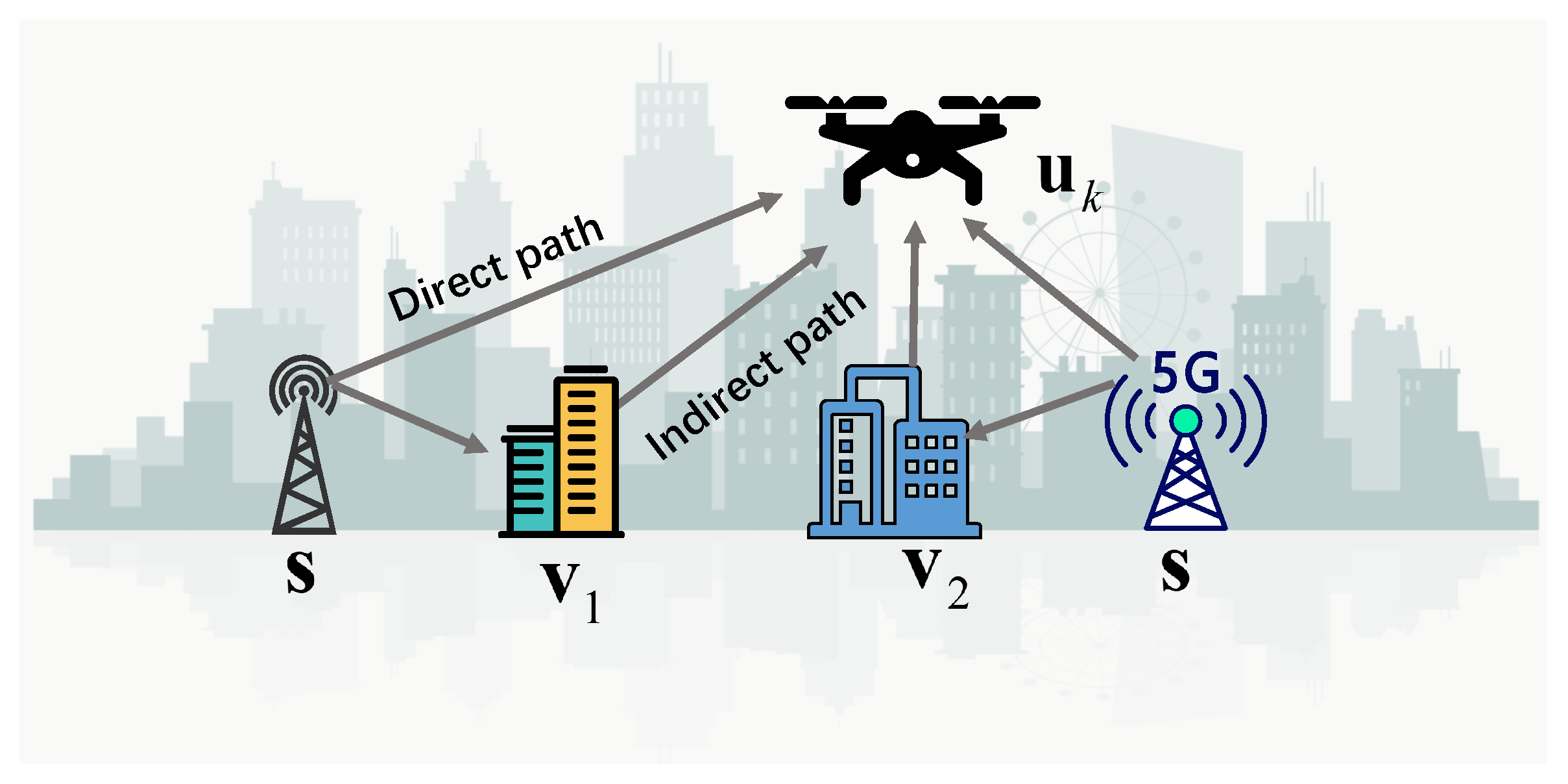
Figure 1 illustrates the sensing geometry. The environment contains a single unknown transmitter $\mathbf{s}\in {\mathbb{R}}^D$ and M stationary scatterers. Under the discrete scattering-center model [30], the channel is assumed to contain one LOS path and M resolved NLOS paths. Each m-th NLOS component ($m=1,\dots ,M$) is modeled as a single-bounce equivalent path associated with a stationary virtual anchor located at ${\mathbf{v}}_m$. Diffuse or unresolved multi-bounce components are absorbed into the measurement noise. The corresponding m-th NLOS path length is therefore given by $\parallel \mathbf{s}-{\mathbf{v}}_m\parallel +\parallel {\mathbf{v}}_m-{\mathbf{u}}_k\parallel$. Delay-domain processing is used to estimate these path lengths. In practice, this requires high-resolution estimators such as Estimation of Signal Parameters via Rotational Invariance Techniques (ESPRIT) and Space Alternating Generalized Expectation Maximization (SAGE) [13,30].

2.1. Multipath Resolvability

A fundamental prerequisite for the proposed framework is the statistical separability of multipath components. To keep the analysis applicable to different SOP waveforms (e.g., LTE and 5G NR), we model the transmitted signal as band-limited, with effective spatial bandwidth ${\mathrm{BW}}_{\mathrm{eff}}$ defined as the root-mean-square bandwidth divided by the speed of light.

The variance of the estimated physical path length, ${\sigma }_m^2=\mathrm{var}\left({\widehat{d}}_{k,m}^{\mathrm{prop}}\right)$, is characterized by the Cramér–Rao lower bound (CRLB):

$${\sigma }_m^2\ge {\displaystyle \frac{1}{8{\pi }^2{\mathrm{BW}}_{\mathrm{eff}}^2{\mathrm{SNR}}_m}},$$

(1)

where ${\mathrm{SNR}}_m$ is the linear signal-to-noise ratio (SNR) of the m-th path.

Spatial Multipath Resolvability: Propagation paths are considered statistically resolvable over the K-epoch window if, for all epochs $k\in \{1,\dots ,K\}$ and all distinct path pairs $(i,j)$, their path-length separation exceeds the corresponding estimation uncertainty:

$$\underset{k}{\min }\underset{i\ne j}{\min }|d_{k,i}^{\mathrm{prop}}-d_{k,j}^{\mathrm{prop}}|>\zeta \sqrt{{\sigma }_i^2+{\sigma }_j^2},$$

(2)

where $d_{k,m}^{\mathrm{prop}}$ denotes the true geometric path length and $\zeta$ is a confidence multiplier.

To derive a waveform-agnostic sufficient condition, define the worst-case ranging uncertainty using ${\mathrm{SNR}}_{\min }\triangleq {\min }_m{\mathrm{SNR}}_m$:

$${\sigma }_{\max }\triangleq {\displaystyle \frac{1}{2\sqrt{2}\pi {\mathrm{BW}}_{\mathrm{eff}}\sqrt{{\mathrm{SNR}}_{\min }}}}.$$

(3)

Since $\sqrt{{\sigma }_i^2+{\sigma }_j^2}\le \sqrt{2}{\sigma }_{\max }$, the sufficient condition for (2) becomes

$$\underset{k}{\min }\underset{i\ne j}{\min }|d_{k,i}^{\mathrm{prop}}-d_{k,j}^{\mathrm{prop}}|>{\displaystyle \frac{\zeta }{2\pi {\mathrm{BW}}_{\mathrm{eff}}\sqrt{{\mathrm{SNR}}_{\min }}}}.$$

(4)

This relationship shows that the minimum resolvable distance is inversely proportional to the spatial bandwidth ($\propto {\mathrm{BW}}_{\mathrm{eff}}^{-1}$). Consequently, wider bandwidths and higher SNRs reduce the resolvable distance threshold and justify the algebraic observation model used below.

2.2. Observation Model

When the resolvability criterion in (4) is satisfied, the extracted multipath components can be associated with the geometric topology. For the m-th NLOS component, the geometric propagation distance is the sum of the transmitter-to-scatterer distance, $d_{m,s}\triangleq \parallel {\mathbf{v}}_m-\mathbf{s}\parallel$, and the scatterer-to-receiver distance, $\parallel {\mathbf{u}}_k-{\mathbf{v}}_m\parallel$.

Because the passive SDR receiver is not synchronized with the SOP transmitter, a clock offset is present. Over the short initialization window, the offset at epoch k is modeled in range units by the first-order polynomial [14,31]

$$t_k=\alpha +\beta {\tau }_k,$$

(5)

where ${\tau }_k$ denotes the elapsed time since the first epoch (${\tau }_1=0$). The vector $\mathbf{c}={[\alpha ,\beta ]}^{\top }$ contains the clock bias and drift, respectively.

Combining geometric path lengths, clock offset, and measurement noise, the pseudorange observations for the LOS path ($m=0$) and the m-th NLOS path are written as

$${\rho }_{k,0}=\parallel {\mathbf{u}}_k-\mathbf{s}\parallel +t_k+{ϵ}_{k,0},$$

(6)

$${\rho }_{k,m}=\parallel {\mathbf{u}}_k-{\mathbf{v}}_m\parallel +d_{m,s}+t_k+{ϵ}_{k,m}.$$

(7)

The noise terms are modeled as independent zero-mean Gaussian random variables, ${ϵ}_{k,m}\sim \mathcal{N}(0,{\sigma }_m^2)$, across epochs k and paths m. The variance ${\sigma }_m^2$ is lower bounded by (1). In practice, ${\sigma }_m^2$ is treated as an effective ranging variance inferred from the estimated SNR and receiver performance, and may exceed the theoretical bound because of residual estimation and modeling errors. Since NLOS components typically experience reflection loss, we adopt a heteroscedastic noise model in which ${\sigma }_m>{\sigma }_0$ for all $m\ge 1$.

2.3. Problem Formulation

Define the geometric state vector as $\mathit{\theta }={[{\mathbf{s}}^{\top },{\mathbf{v}}_1^{\top },\dots ,{\mathbf{v}}_M^{\top }]}^{\top }\in {\mathbb{R}}^{(M+1)D}.$ For each path m, stack the pseudorange measurements over the K epochs into ${\mathbf{y}}_m={[{\rho }_{1,m},\dots ,{\rho }_{K,m}]}^{\top }.$

Collecting all paths yields the aggregate observation vector $\mathbf{y}\triangleq {[{\mathbf{y}}_0^{\top },\dots ,{\mathbf{y}}_M^{\top }]}^{\top },$ which leads to the compact model

$$\mathbf{y}=\mathbf{d}\left(\mathit{\theta }\right)+\mathbf{A}\mathbf{c}+\mathit{ϵ}.$$

(8)

Here, $\mathbf{d}\left(\mathit{\theta }\right)={[{\mathbf{d}}_0^{\top },\dots ,{\mathbf{d}}_M^{\top }]}^{\top }$ denotes the stacked vector of noise-free geometric ranges, with

$${\mathbf{d}}_0\left(\mathit{\theta }\right)={\left[\parallel {\mathbf{u}}_1-\mathbf{s}\parallel ,\dots ,\parallel {\mathbf{u}}_K-\mathbf{s}\parallel \right]}^{\top },$$

(9)

$${\mathbf{d}}_m\left(\mathit{\theta }\right)={\left[\parallel {\mathbf{u}}_1-{\mathbf{v}}_m\parallel +\parallel {\mathbf{v}}_m-\mathbf{s}\parallel ,\dots ,\parallel {\mathbf{u}}_K-{\mathbf{v}}_m\parallel +\parallel {\mathbf{v}}_m-\mathbf{s}\parallel \right]}^{\top },m\ge 1.$$

(10)

The clock coefficient matrix is $\mathbf{A}={\mathbf{1}}_{M+1}\otimes [{\mathbf{1}}_K,\mathit{\tau }],$ where $\mathit{\tau }={[{\tau }_1,\dots ,{\tau }_K]}^{\top }$. The composite noise vector follows $\mathit{ϵ}\sim \mathcal{N}(\mathbf{0},{\mathbf{W}}^{-1})$, where the precision matrix is

$$\mathbf{W}=\mathrm{diag}\left({\sigma }_0^{-2}{\mathbf{I}}_K,{\sigma }_1^{-2}{\mathbf{I}}_K,\dots ,{\sigma }_M^{-2}{\mathbf{I}}_K\right).$$

(11)

Over the short initialization interval, the per-path SNR, and hence ${\sigma }_m^2$, is assumed quasi-static. This yields the block-diagonal precision structure in (11). The formulation can be extended in a straightforward manner to epoch-dependent weights ${\sigma }_{k,m}^2$ if needed.

The navigation bootstrapping problem is therefore formulated as a maximum-likelihood estimation (MLE) problem:

$$\underset{\mathit{\theta },\mathbf{c}}{\min }Q(\mathit{\theta },\mathbf{c})=\frac{1}{2}{\parallel \mathbf{y}-\mathbf{d}\left(\mathit{\theta }\right)-\mathbf{A}\mathbf{c}\parallel }_{\mathbf{W}}^2.$$

(12)

3. Observability and Performance Analysis

This section derives theoretical performance bounds for the estimation problem through the FIM and the corresponding CRLB. The analysis links signal-level ranging precision to the spatial sensing geometry and identifies the conditions under which resolvable NLOS paths provide sufficient diversity for local observability.

3.1. Joint FIM and CRLB Formulation

Define the full parameter vector as $\mathbf{x}={[{\mathit{\theta }}^{\top },{\mathbf{c}}^{\top }]}^{\top }$. Let $\mathbf{J}=[\mathbf{G},\mathbf{A}]$ denote the Jacobian matrix, where $\mathbf{G}=\partial \mathbf{d}\left(\mathit{\theta }\right)/\partial \mathit{\theta }$ is the geometric sensitivity matrix. The joint FIM is then

$$\mathbf{F}={\mathbf{J}}^{\top }\mathbf{W}\mathbf{J}=\left[\begin{array}{cc}{\mathbf{G}}^{\top }\mathbf{W}\mathbf{G}& {\mathbf{G}}^{\top }\mathbf{W}\mathbf{A}\\ {\mathbf{A}}^{\top }\mathbf{W}\mathbf{G}& {\mathbf{A}}^{\top }\mathbf{W}\mathbf{A}\end{array}\right],\mathrm{Cov}\left(\widehat{\mathbf{x}}\right)⪰{\mathbf{F}}^{-1}.$$

(13)

The matrix ${\mathbf{A}}^{\top }\mathbf{W}\mathbf{A}$ is invertible provided that the time-tag set contains at least two distinct values.

3.2. Clock-Null Projection and Geometric CRLB

For fixed geometry $\mathit{\theta }$, minimizing (12) with respect to the linear clock parameters $\mathbf{c}$ yields

$$\widehat{\mathbf{c}}\left(\mathit{\theta }\right)={\left({\mathbf{A}}^{\top }\mathbf{W}\mathbf{A}\right)}^{-1}{\mathbf{A}}^{\top }\mathbf{W}\left(\mathbf{y}-\mathbf{d}\left(\mathit{\theta }\right)\right).$$

(14)

Define the whitened residual vector and the whitened Jacobians as

$$\tilde{\mathbf{r}}\left(\mathit{\theta }\right)={\mathbf{W}}^{1/2}(\mathbf{y}-\mathbf{d}\left(\mathit{\theta }\right)),\tilde{\mathbf{G}}={\mathbf{W}}^{1/2}\mathbf{G},\tilde{\mathbf{A}}={\mathbf{W}}^{1/2}\mathbf{A}.$$

The orthogonal projector onto the subspace orthogonal to the clock dynamics is ${\mathbf{P}}_A=\mathbf{I}-\tilde{\mathbf{A}}{\left({\tilde{\mathbf{A}}}^{\top }\tilde{\mathbf{A}}\right)}^{-1}{\tilde{\mathbf{A}}}^{\top }.$ Substituting $\widehat{\mathbf{c}}\left(\mathit{\theta }\right)$ into the objective eliminates the explicit timing parameters and yields the concentrated cost

$$Q_{\mathrm{eff}}\left(\mathit{\theta }\right)={\displaystyle \frac{1}{2}}{∥{\mathbf{P}}_A\tilde{\mathbf{r}}\left(\mathit{\theta }\right)∥}_2^2.$$

(15)

The effective geometric FIM is obtained from the Schur complement of the clock-information block:

$${\mathbf{F}}_{\mathit{\theta }}^{\mathrm{eff}}={\tilde{\mathbf{G}}}^{\top }{\mathbf{P}}_A\tilde{\mathbf{G}}={\mathbf{G}}^{\top }\mathbf{W}\mathbf{G}-{\mathbf{G}}^{\top }\mathbf{W}\mathbf{A}{\left({\mathbf{A}}^{\top }\mathbf{W}\mathbf{A}\right)}^{-1}{\mathbf{A}}^{\top }\mathbf{W}\mathbf{G},$$

(16)

$${\mathrm{CRLB}}_{\mathit{\theta }}={\left({\mathbf{F}}_{\mathit{\theta }}^{\mathrm{eff}}\right)}^{-1}.$$

(17)

A useful property of this formulation is the monotonic increase of geometric information. For any resolvable single-bounce path m added to an existing path set $\mathcal{P}$,

$${\mathbf{F}}_{\mathit{\theta }}^{\mathrm{eff}}(\mathcal{P}\cup \left\{m\right\})⪰{\mathbf{F}}_{\mathit{\theta }}^{\mathrm{eff}}\left(\mathcal{P}\right).$$

(18)

This inequality is strict whenever the newly added path provides linearly independent constraints after clock projection. Hence, additional resolvable reflections do not reduce the effective geometric information and may improve it.

3.3. Analysis of Observability and Degradation

We next analyze the local observability and geometric degeneracy of the projected state $\mathit{\theta }={[{\mathbf{s}}^{\top },{\mathbf{v}}_1^{\top },\dots ,{\mathbf{v}}_M^{\top }]}^{\top }.$

3.3.1. Local Observability via Jacobian Analysis

Define the unit direction vectors

$${\widehat{\mathbf{h}}}_{k,s}:={\displaystyle \frac{{\mathbf{u}}_k-\mathbf{s}}{\parallel {\mathbf{u}}_k-\mathbf{s}\parallel }},{\widehat{\mathbf{a}}}_{k,m}:={\displaystyle \frac{{\mathbf{v}}_m-{\mathbf{u}}_k}{\parallel {\mathbf{v}}_m-{\mathbf{u}}_k\parallel }},{\widehat{\mathbf{b}}}_m:={\displaystyle \frac{{\mathbf{v}}_m-\mathbf{s}}{\parallel {\mathbf{v}}_m-\mathbf{s}\parallel }}.$$

(19)

For the LOS path, the sensitivity row is ${\nabla }_{\mathit{\theta }}{\rho }_{k,0}=\left[-{\widehat{\mathbf{h}}}_{k,s}^{\top },{\mathbf{0}}^{\top },\dots ,{\mathbf{0}}^{\top }\right].$ For the m-th NLOS path, the sensitivity couples the source to the corresponding reflector:

$${\nabla }_{\mathit{\theta }}{\rho }_{k,m}=\left[-{\widehat{\mathbf{b}}}_m^{\top },{\mathbf{0}}^{\top },\dots ,\underset{\mathrm{Reflector}m}{\underbrace{{\widehat{\mathbf{a}}}_{k,m}^{\top }+{\widehat{\mathbf{b}}}_m^{\top }}},\dots ,{\mathbf{0}}^{\top }\right].$$

(20)

3.3.2. Dimensional Analysis and Minimum Epochs

A necessary condition for solvability follows from a Degree-of-Freedom (DoF) count. Since $\mathrm{rank}\left(\mathbf{A}\right)=2$, the clock contributes two identifiable parameters. For planar geometry ($D=2$),

$$\begin{array}{cc}\hfill (M+1)K& \ge \underset{\mathrm{Reflectors}}{\underbrace{2M}}+\underset{\mathrm{Source}}{\underbrace{2}}+\underset{\mathrm{Clock}}{\underbrace{2}}\hfill \\ \hfill \Rightarrow K& \ge ⌈2+{\displaystyle \frac{2}{M+1}}⌉.\hfill \end{array}$$

(21)

Thus, $K=3$ epochs are sufficient at the level of necessary dimensional consistency.

3.3.3. Geometric Singularities

Even when $K\ge 3$, certain sensing geometries can still induce rank deficiency and cause the smallest eigenvalue of the effective FIM to vanish. For clarity, we first consider the whitened case with $\mathbf{W}=\mathbf{I}$; the same analysis extends to the weighted case after pre-whitening.

LOS Degeneration: Let ${\phi }_{k,s}\triangleq \angle ({\mathbf{u}}_k-\mathbf{s})$, so that ${\widehat{\mathbf{h}}}_{k,s}={[\cos {\phi }_{k,s},\sin {\phi }_{k,s}]}^{\top }$. The LOS information matrix for $\mathbf{s}$ is

$${\mathcal{I}}^{\mathrm{LOS}}=\sum _{k=1}^K{\widehat{\mathbf{h}}}_{k,s}{\widehat{\mathbf{h}}}_{k,s}^{\top }.$$

(22)

Using standard trigonometric identities, the eigenvalues are

$${\lambda }_{\pm }={\displaystyle \frac{K}{2}}\pm {\displaystyle \frac{1}{2}}\sqrt{{\left({\displaystyle \sum _{k=1}^K}\cos 2{\phi }_{k,s}\right)}^2+{\left({\displaystyle \sum _{k=1}^K}\sin 2{\phi }_{k,s}\right)}^2}.$$

(23)

Let $S=K/2$ and $R={\displaystyle \frac{1}{2}}\left|{\sum }_{k=1}^K{e}^{\mathrm{j}2{\phi }_{k,s}}\right|$. Then the condition number is

$$\kappa \left({\mathcal{I}}^{\mathrm{LOS}}\right)={\displaystyle \frac{{\lambda }_{+}}{{\lambda }_{-}}}={\displaystyle \frac{S+R}{S-R}}.$$

(24)

The matrix becomes singular as $R\to S$, which implies $\kappa \to \infty$. This occurs under pure radial motion, where the LOS bearing remains nearly constant over the observation interval. In that case, the vectors ${\widehat{\mathbf{h}}}_{k,s}$ become collinear and the cross-range direction is unobservable.

NLOS Degeneration: For the m-th NLOS path, define the bistatic angle deviation as ${\varphi }_{k,m}\triangleq {\mathrm{wrap}}_{(-\pi ,\pi ]}({\phi }_{k,m}-{\vartheta }_m).$ The per-epoch Gram matrix is

$${\mathbf{\Gamma }}_{k,m}=\left[\begin{array}{cc}1& -2{\sin }^2({\varphi }_{k,m}/2)\\ -2{\sin }^2({\varphi }_{k,m}/2)& 4{\sin }^2({\varphi }_{k,m}/2)\end{array}\right].$$

(25)

Its determinant is $\det \left({\mathbf{\Gamma }}_{k,m}\right)={\sin }^2{\varphi }_{k,m}$, which vanishes in two degenerate cases:

• Specular alignment (${\varphi }_{k,m}\to 0$): The receiver, transmitter, and reflector are nearly collinear, so the bistatic range becomes weakly sensitive to reflector motion transverse to the line of sight.
• Backscatter geometry (${\varphi }_{k,m}\to \pi$): The receiver lies approximately on the segment between the transmitter and reflector.

A local expansion around these points shows that the smallest eigenvalue decays quadratically: ${\lambda }_{\min ,k}\propto {\varphi }_{k,m}^2\mathrm{near}\mathrm{alignment},\mathrm{and}{\lambda }_{\min ,k}\propto (\pi -|{\varphi }_{k,m}{\left|\right)}^2\mathrm{near}\mathrm{backscatter}.$

Cumulative Information and Diversity: Summing over K epochs gives ${\mathbf{F}}_m={\sum }_{k=1}^K{\mathbf{\Gamma }}_{k,m}$. Let ${\psi }_m\triangleq {\sum }_{k=1}^K{\sin }^2({\varphi }_{k,m}/2).$ Then

$${\mathbf{F}}_m=\left[\begin{array}{cc}K& -2{\psi }_m\\ -2{\psi }_m& 4{\psi }_m\end{array}\right].$$

(26)

This matrix is singular only when ${\psi }_m\in \{0,K\}$, that is, when the geometry remains degenerate across all epochs. Define the diversity ratio $\varpi \triangleq {\psi }_m/K\in [0,1]$. The resulting condition number is

$$\kappa \left({\mathbf{F}}_m\right)={\displaystyle \frac{1+4\varpi +\sqrt{1-8\varpi +32{\varpi }^2}}{1+4\varpi -\sqrt{1-8\varpi +32{\varpi }^2}}}.$$

(27)

The minimum value is ${\kappa }_{\min }\approx 2.618$ at ${\varpi }^{★}=1/6$. Therefore, maintaining $\varpi$ away from 0 and 1 is desirable in trajectory design. In the absence of prior maps, this motivates angularly diverse maneuvers such as arcs, polylines, or figure-eight trajectories rather than extended near-radial motion.

3.4. Stability and Model Sensitivity

Oscillator frequency aging $\eta$ introduces a quadratic drift term ${\displaystyle \frac{1}{2}}\eta {\tau }^2$. To keep this bias small relative to the ranging noise floor ${\sigma }_{\rho }$, the observation interval T should satisfy

$${\displaystyle \frac{\left|\eta \right|}{2}}{T}^2\le c_{\mathrm{tol}}{\sigma }_{\rho },$$

(28)

where $c_{\mathrm{tol}}\ll 1$ is a tolerance factor. This inequality determines the admissible integration interval: high-stability oscillators permit longer windows, whereas lower-grade oscillators require shorter windows to limit the accumulation of quadratic drift.

To assess robustness to deviations from the point-scattering model, consider a Jacobian perturbation satisfying $\parallel \Delta \tilde{\mathbf{G}}\parallel \le {\Delta }_{\mathrm{geo}}$. This induces an FIM perturbation bounded by $\parallel \Delta \mathbf{F}\parallel \le 2\parallel \tilde{\mathbf{G}}\parallel {\Delta }_{\mathrm{geo}}$. Using a Neumann-series argument, the covariance degradation satisfies

$$∥{({\mathbf{F}}_{\mathit{\theta }}^{\mathrm{eff}}+\Delta \mathbf{F})}^{-1}-{\mathbf{F}}_{\mathit{\theta }}^{\mathrm{eff}-1}∥\le {\displaystyle \frac{\parallel {\mathbf{F}}_{\mathit{\theta }}^{\mathrm{eff}-1}{\parallel }^2\parallel \Delta \mathbf{F}\parallel }{1-\parallel {\mathbf{F}}_{\mathit{\theta }}^{\mathrm{eff}-1}\parallel \parallel \Delta \mathbf{F}\parallel }}.$$

(29)

This bound shows that, in the small-perturbation regime, estimation error grows approximately linearly with the geometric mismatch ${\Delta }_{\mathrm{geo}}$. Increasing the smallest eigenvalue of ${\mathbf{F}}_{\mathit{\theta }}^{\mathrm{eff}}$ therefore helps limit the amplification of modeling errors.

4. Two-Stage Estimation Framework

The joint MLE in (12) is a high-dimensional nonconvex problem and is susceptible to local minima when infrastructure parameters are unknown. To address this difficulty, we adopt a two-stage hierarchical solver:

• Stage I (Algebraic Initialization): A non-iterative estimate is obtained through measurement differencing and squared-range linearization, providing a robust initialization under large initial uncertainty.
• Stage II (Manifold Refinement): The CNP formulation is used for iterative optimization in the clock-eliminated subspace, refining the estimate toward the theoretical bound derived in Section 3.

4.1. Stage I: Algebraic Initialization

Stage I decouples the parameters and reformulates the nonlinear observation model into a pseudo-linear system, yielding a closed-form initial estimate ${\widehat{\mathit{\theta }}}^{\left(0\right)}$.

4.1.1. Differencing and Bias Elimination

To eliminate the static clock bias $\alpha$, measurements are differenced relative to the first epoch ($k=1$). Defining $\Delta {\tau }_k\triangleq {\tau }_k-{\tau }_1$, (6) and (7) become

$$\Delta {\rho }_{k,0}\triangleq {\rho }_{k,0}-{\rho }_{1,0}=(d_{k,s}-d_{1,s})+\beta \Delta {\tau }_k+\Delta {ϵ}_{k,0},$$

(30a)

$$\Delta {\rho }_{k,m}\triangleq {\rho }_{k,m}-{\rho }_{1,m}=(d_{k,m}-d_{1,m})+\beta \Delta {\tau }_k+\Delta {ϵ}_{k,m},$$

(30b)

where $d_{k,s}=\parallel {\mathbf{u}}_k-\mathbf{s}\parallel$ and $d_{k,m}=\parallel {\mathbf{u}}_k-{\mathbf{v}}_m\parallel +\parallel {\mathbf{v}}_m-\mathbf{s}\parallel$.

Assuming independent epoch noise, the differenced terms $\Delta {ϵ}_{k,m}={ϵ}_{k,m}-{ϵ}_{1,m}$ become temporally correlated. Stacking the differenced noise for $k\in \{2,\dots ,K\}$ gives $\Delta {\mathit{ϵ}}_m\sim \mathcal{N}(\mathbf{0},{\mathbf{\Sigma }}_{\Delta ,m}),$ with coiance

$${\mathbf{\Sigma }}_{\Delta ,m}={\sigma }_m^2\left({\mathbf{I}}_{K-1}+\mathbf{1}{\mathbf{1}}^{\top }\right).$$

(31)

A rank-one update gives the closed-form inverse

$${\mathbf{\Sigma }}_{\Delta ,m}^{-1}={\displaystyle \frac{1}{{\sigma }_m^2}}\left({\mathbf{I}}_{K-1}-{\displaystyle \frac{1}{K}}\mathbf{1}{\mathbf{1}}^{\top }\right),$$

(32)

which enables exact Generalized Least-Squares (GLS) weighting with low computational cost. The global differenced covariance is therefore ${\mathbf{\Sigma }}_{\Delta }=\mathrm{blkdiag}({\mathbf{\Sigma }}_{\Delta ,0},\dots ,{\mathbf{\Sigma }}_{\Delta ,M}).$

4.1.2. Linearization and Auxiliary Variable Construction

For the LOS channel, use the identity $\parallel {\mathbf{u}}_k{-\mathbf{s}\parallel }^2-{\parallel {\mathbf{u}}_1-\mathbf{s}\parallel }^2=d_{k,s}^2-d_{1,s}^2.$ Substituting $d_{k,s}=\Delta {\rho }_{k,0}-\beta \Delta {\tau }_k+d_{1,s}-\Delta {ϵ}_{k,0}$ yields

$$\begin{array}{cc}\hfill \parallel {\mathbf{u}}_k{\parallel }^2-{\parallel {\mathbf{u}}_1\parallel }^2-{(\Delta {\rho }_{k,0})}^2=& 2{({\mathbf{u}}_k-{\mathbf{u}}_1)}^{\top }\mathbf{s}-2\Delta {\rho }_{k,0}\Delta {\tau }_k\beta \hfill \\ \hfill & +{(\Delta {\tau }_k)}^2{\beta }^2-2\Delta {\tau }_k\beta d_{1,s}+2\Delta {\rho }_{k,0}{d}_{1,s}-\mathcal{O}(\Delta {ϵ}_{k,0}),\hfill \end{array}$$

(33)

where the first-order approximation of the noise-coupling term is

$$\begin{array}{cc}\hfill \mathcal{O}(\Delta {ϵ}_{k,0})& =\left(-2\Delta {\tau }_k\beta +2d_{1,s}+2\Delta {\rho }_{k,0}\right)\Delta {ϵ}_{k,0}+{(\Delta {ϵ}_{k,0})}^2\hfill \\ \hfill & \approx B_{k,0}\Delta {ϵ}_{k,0}.\hfill \end{array}$$

(34)

Define $B_{k,0}\triangleq -2\Delta {\tau }_k\beta +2d_{1,s}+2\Delta {\rho }_{k,0}$. Similarly, for the m-th NLOS path,

$$\begin{array}{cc}\hfill \parallel {\mathbf{u}}_k{\parallel }^2-{\parallel {\mathbf{u}}_1\parallel }^2-{(\Delta {\rho }_{k,m})}^2=& 2{({\mathbf{u}}_k-{\mathbf{u}}_1)}^{\top }{\mathbf{v}}_m-2\Delta {\rho }_{k,m}\Delta {\tau }_k\beta \hfill \\ \hfill & +{(\Delta {\tau }_k)}^2{\beta }^2-2\Delta {\tau }_k\beta d_{1,m}+2\Delta {\rho }_{k,m}{d}_{1,m}-\mathcal{O}(\Delta {ϵ}_{k,m}),\hfill \end{array}$$

(35)

with $\mathcal{O}(\Delta {ϵ}_{k,m})\approx B_{k,m}\Delta {ϵ}_{k,m}$ and $B_{k,m}\triangleq -2\Delta {\tau }_k\beta +2d_{1,m}+2\Delta {\rho }_{k,m}.$

To obtain a standard linear form, introduce the auxiliary variables

$$p={\beta }^2,{\xi }_s=\beta d_{1,s},{\xi }_m=\beta d_{1,m}.$$

(36)

4.1.3. Construction and Solution of the Linear Equation System

Collecting the $(K-1)$ Equations from (33) and (35) yields the pseudo-linear systems

$${\mathbf{N}}_0\mathbf{z}-{\mathbf{B}}_0{\mathit{ϵ}}_0={\ell }_0,{\mathbf{N}}_m\mathbf{z}-{\mathbf{B}}_m{\mathit{ϵ}}_m={\ell }_m.$$

(37)

The extended state vector is

$$\mathbf{z}={[{\mathbf{s}}^{\top },{\mathbf{v}}_1^{\top },\dots ,{\mathbf{v}}_M^{\top },\beta ,p,{\xi }_s,{\xi }_1,\dots ,{\xi }_M,d_{1,s},d_{1,1},\dots ,d_{1,M}]}^{\top }.$$

(38)

The measurement vectors and noise coefficient matrices are

$${\ell }_0={\left[\parallel {\mathbf{u}}_2{\parallel }^2-{\parallel {\mathbf{u}}_1\parallel }^2-{(\Delta {\rho }_{2,0})}^2,\dots \right]}^{\top },$$

(39a)

$${\ell }_m={\left[\parallel {\mathbf{u}}_2{\parallel }^2-{\parallel {\mathbf{u}}_1\parallel }^2-{(\Delta {\rho }_{2,m})}^2,\dots \right]}^{\top },$$

(39b)

$${\mathbf{B}}_0=\mathrm{diag}(B_{2,0},\dots ,B_{K,0}),$$

(39c)

$${\mathbf{B}}_m=\mathrm{diag}(B_{2,m},\dots ,B_{K,m}).$$

(39d)

The row vectors ${\mathbf{n}}_{k,0}$ and ${\mathbf{n}}_{k,m}$ are constructed so as to align with $\mathbf{z}$:

$${\mathbf{n}}_{k,0}={\left[2{({\mathbf{u}}_k-{\mathbf{u}}_1)}^{\top },{\mathbf{0}}_{\mathrm{refl}}^{\top },-2\Delta {\rho }_{k,0}\Delta {\tau }_k,{(\Delta {\tau }_k)}^2,-2\Delta {\tau }_k,{\mathbf{0}}_{\xi }^{\top },2\Delta {\rho }_{k,0},{\mathbf{0}}_d^{\top }\right]}^{\top },$$

(40a)

$${\mathbf{n}}_{k,m}={\left[{\mathbf{0}}^{\top },\dots ,2{({\mathbf{u}}_k-{\mathbf{u}}_1)}^{\top },\dots ,-2\Delta {\rho }_{k,m}\Delta {\tau }_k,{(\Delta {\tau }_k)}^2,0,\dots ,-2\Delta {\tau }_k,\dots ,2\Delta {\rho }_{k,m}\right]}^{\top }.$$

(40b)

Aggregating all paths gives the unified system

$$\mathbf{N}\mathbf{z}-\mathbf{B}{\mathit{ϵ}}_{\Delta }=\ell ,$$

(41)

where $\mathbf{B}=\mathrm{diag}({\mathbf{B}}_0,{\mathbf{B}}_1,\dots ,{\mathbf{B}}_M)$ and $\mathbf{N}={[{\mathbf{N}}_0^{\top },{\mathbf{N}}_1^{\top },\dots ,{\mathbf{N}}_M^{\top }]}^{\top }$. The weighted least-squares (WLS) solution is

$$\widehat{\mathbf{z}}={\left({\mathbf{N}}^{\top }{\mathbf{W}}_{\Delta }\mathbf{N}\right)}^{-1}{\mathbf{N}}^{\top }{\mathbf{W}}_{\Delta }\ell ,$$

(42)

where the ideal weight matrix is ${\mathbf{W}}_{\Delta }={\left(\mathbf{B}{\mathbf{\Sigma }}_{\Delta }{\mathbf{B}}^{\top }\right)}^{-1}$.

Since $\mathbf{B}$ depends on $(\beta ,d_{1,·})$, we use a plug-in reweighting strategy: (i) solve (42) once with $\mathbf{B}=\mathbf{I}$ and ${\mathbf{\Sigma }}_{\Delta }$ given by (31); (ii) compute $\mathbf{B}$ from the coarse solution and perform one reweighted WLS pass. This two-pass procedure remains closed-form and provides a reliable initializer for Stage II.

The fixed clock offset $\alpha$ is then estimated as

$$\widehat{\alpha }={\displaystyle \frac{1}{K}}\sum _{k=1}^K\left({\rho }_{k,0}-\parallel {\mathbf{u}}_k-\widehat{\mathbf{s}}\parallel -\widehat{\beta }{\tau }_k\right).$$

(43)

This initialization improves numerical stability for the subsequent nonconvex optimization. Moreover, Stage I does not fundamentally rely on the single-bounce assumption. In a multi-bounce scenario, the total propagation delay can be written as

$${\rho }_{k,m}=\parallel {\mathbf{u}}_k-{\mathbf{v}}_m\parallel +d_{m,\mathrm{bias}}+t_k+{ϵ}_{k,m},$$

(44)

where ${\mathbf{v}}_m$ denotes the terminal reflector position and $d_{m,\mathrm{bias}}$ captures the constant delay contributed by the preceding segments. Inter-epoch differencing removes the static bias term $d_{m,\mathrm{bias}}$. As a result, Stage I depends mainly on the terminal reflection geometry and is therefore less sensitive to the number of preceding bounces. In this sense, the single-bounce assumption is sufficient for topology interpretation but not necessary for initialization stability.

4.2. Stage II: Manifold Refinement

Starting from the initial estimate ${\widehat{\mathit{\theta }}}^{\left(0\right)}$, Stage II minimizes the concentrated likelihood (15) to refine the geometric parameters. Defining the whitened residual $\tilde{\mathbf{r}}\left(\mathit{\theta }\right)={\mathbf{W}}^{1/2}(\mathbf{y}-\mathbf{d}\left(\mathit{\theta }\right)),$ the objective becomes

$$\widehat{\mathit{\theta }}=\arg \underset{\mathit{\theta }}{\min }{\displaystyle \frac{1}{2}}{∥{\mathbf{P}}_A\tilde{\mathbf{r}}\left(\mathit{\theta }\right)∥}_2^2.$$

(45)

The update $\Delta \mathit{\theta }$ is computed using a Levenberg–Marquardt scheme:

$$({\tilde{\mathbf{G}}}_t^{\top }{\mathbf{P}}_A{\tilde{\mathbf{G}}}_t+{\nu }_t\mathbf{I})\Delta \mathit{\theta }={\tilde{\mathbf{G}}}_t^{\top }{\mathbf{P}}_A\tilde{\mathbf{r}}\left({\mathit{\theta }}_t\right),$$

(46)

where ${\nu }_t$ is the damping factor.

In our implementation, the refinement terminates when the relative change in the parameter vector falls below ${10}^{-6}$ or when the maximum number of iterations ($N_{\max }=20$) is reached. This setting was sufficient in our experiments and allowed the estimator to approach the CRLB under the stated regularity conditions. The initial damping factor is set to ${\nu }_0={10}^{-3}\max (\mathrm{diag}({\tilde{\mathbf{G}}}_0^{\top }{\mathbf{P}}_A{\tilde{\mathbf{G}}}_0)),$ which stabilizes the initial descent without overly restricting the step size. During optimization, ${\nu }_t$ is adjusted according to the gain ratio between the actual and predicted reduction in the objective. When an update decreases the residual, ${\nu }_t$ is reduced to move toward the Gauss–Newton regime; otherwise, it is increased to enforce a more gradient-descent-like step. In the Gauss–Newton regime (${\nu }_t\to 0$), the local Hessian approaches the effective FIM in (16), which explains the asymptotic efficiency of the estimator under the stated regularity conditions. After convergence, the clock parameters are recovered by

$$\widehat{\mathbf{c}}={({\mathbf{A}}^{\top }\mathbf{W}\mathbf{A})}^{-1}{\mathbf{A}}^{\top }\mathbf{W}(\mathbf{y}-\mathbf{d}(\widehat{\mathit{\theta }})).$$

(47)

4.3. Error Propagation and Asymptotic Optimality

The hierarchical structure of the proposed framework allows the initial algebraic estimate to be refined toward the theoretical accuracy limit. In Stage I, the initializer ${\widehat{\mathit{\theta }}}^{\left(0\right)}$ is obtained from the pseudo-linear system in (42). Under the Gauss–Markov theorem, the covariance of the extended WLS estimate is approximated by

$$\mathrm{Cov}\left(\widehat{\mathbf{z}}\right)\approx {\left({\mathbf{N}}^{\top }{\mathbf{W}}_{\Delta }\mathbf{N}\right)}^{-1}.$$

(48)

The geometric uncertainty of the initialization, denoted by ${\mathbf{P}}_{\mathit{\theta }}^{\left(0\right)}$, is given by the corresponding $(M+1)D\times (M+1)D$ sub-block of $\mathrm{Cov}\left(\widehat{\mathbf{z}}\right)$. Although Stage I is robust to large initial uncertainty and does not require a prior guess, ${\widehat{\mathit{\theta }}}^{\left(0\right)}$ may still contain structural bias due to the linearization and the noise-coupling terms embedded in $\mathbf{B}$.

Stage II performs maximum-likelihood refinement directly on the nonlinear manifold. By minimizing $Q_{\mathrm{eff}}\left(\mathit{\theta }\right)$ in (15), the estimator corrects the algebraic bias introduced in Stage I. Once ${\nu }_t$ becomes small and the iteration enters the Gauss–Newton regime, the local Hessian aligns with the effective geometric FIM ${\mathbf{F}}_{\mathit{\theta }}^{\mathrm{eff}}$. Accordingly, the asymptotic covariance of the refined estimate satisfies

$$\mathrm{Cov}(\widehat{\mathit{\theta }})\approx {({\tilde{\mathbf{G}}}^{\top }{\mathbf{P}}_A\tilde{\mathbf{G}})}^{-1}={\mathrm{CRLB}}_{\mathit{\theta }}.$$

(49)

This relationship indicates that the proposed two-stage framework is asymptotically efficient under the assumed local regularity conditions. In this sense, the estimator transitions from a robust closed-form initializer to a statistically efficient nonlinear refinement.

The convergence behavior of the manifold refinement is further shaped by both physical constraints and geometric conditioning. Let ${\mathit{\theta }}^{★}$ denote a local minimizer of $Q_{\mathrm{eff}}\left(\mathit{\theta }\right)$, and assume that $Q_{\mathrm{eff}}$ is twice continuously differentiable. A standard Newton–Kantorovich argument gives a sufficient local condition for the convergence of Gauss–Newton/Levenberg–Marquardt (LM) iterations. Assume that ${\nabla }^2{Q}_{\mathrm{eff}}\left(\mathit{\theta }\right)$ is Lipschitz continuous with constant L in a neighborhood of the initial point ${\mathit{\theta }}_0={\widehat{\mathit{\theta }}}^{\left(0\right)}$, and that ${\nabla }^2{Q}_{\mathrm{eff}}\left({\mathit{\theta }}_0\right)\succ \mathbf{0}$. Define

$$\chi \triangleq {∥{\nabla }^2{Q}_{\mathrm{eff}}{\left({\mathit{\theta }}_0\right)}^{-1}\nabla Q_{\mathrm{eff}}\left({\mathit{\theta }}_0\right)∥}_2,h\triangleq L{∥{\nabla }^2{Q}_{\mathrm{eff}}{\left({\mathit{\theta }}_0\right)}^{-1}∥}_2\chi .$$

(50)

If $h\le \frac{1}{2}$, the LM iterations are locally guaranteed to converge to a unique stationary point within that neighborhood.

In the present setting, the scale of the initialization error, and thus $\chi$, is driven by the ranging uncertainty ${\sigma }_m^2$. Combined with (1), this indicates that larger spatial bandwidth and higher SNR reduce the expected initialization error and increase the likelihood that ${\widehat{\mathit{\theta }}}^{\left(0\right)}$ lies within the local convergence basin.

4.4. Computational Complexity

Computational feasibility is an important consideration for real-time onboard implementation on SWaP-constrained UAV platforms. By exploiting the sparsity and algebraic structure of the sensing geometry, the proposed implementation avoids dense cubic scaling in M and admits overall complexity that is linear in K and M for fixed spatial dimension D.

Let K denote the number of epochs, M the number of resolved NLOS paths, and $D\in \{2,3\}$ the spatial dimension. The number of observations is $N_y=(M+1)(K-1)$ in Stage I and $N_y=(M+1)K$ in Stage II.

4.4.1. Complexity of Stage I: Algebraic Initialization

The Stage-I estimator solves the normal equations $\left({\mathbf{N}}^{\top }{\mathbf{W}}_{\Delta }\mathbf{N}\right)\widehat{\mathbf{z}}={\mathbf{N}}^{\top }{\mathbf{W}}_{\Delta }\ell .$ The extended state vector has dimension $N_z=(M+1)D+2M+4$. A naive dense inversion would require $\mathcal{O}\left(N_z^3\right)$ operations. However, once the common source and clock variables are isolated, the measurements decouple across reflectors.

As a result, the information matrix ${\mathbf{H}}_I\triangleq {\mathbf{N}}^{\top }{\mathbf{W}}_{\Delta }\mathbf{N}$ has the block-arrowhead structure

$${\mathbf{H}}_I=\left[\begin{array}{cccc}{\mathbf{H}}_{cc}& {\mathbf{H}}_{c1}& \dots & {\mathbf{H}}_{cM}\\ {\mathbf{H}}_{c1}^{\top }& {\mathbf{H}}_{11}& \mathbf{0}& \mathbf{0}\\ ⋮& \mathbf{0}& \ddots & \mathbf{0}\\ {\mathbf{H}}_{cM}^{\top }& \mathbf{0}& \mathbf{0}& {\mathbf{H}}_{MM}\end{array}\right].$$

(51)

Here, ${\mathbf{H}}_{cc}$ contains the common variables, while the ${\mathbf{H}}_{mm}$ blocks are low-dimensional reflector-specific blocks. By using the block Schur complement, inversion reduces to the inversion of ${\mathbf{H}}_{cc}$ together with M small independent blocks. Since D is at most 3, the dominant cost comes from constructing ${\mathbf{H}}_I$, which scales as $\mathcal{O}\left(KM{D}^2\right)$. Thus, for fixed D, Stage I has linear complexity in K and M.

4.4.2. Complexity of Stage II: Manifold Refinement

In Stage II, the dominant computation in each LM iteration is the solution of $({\tilde{\mathbf{G}}}^{\top }{\mathbf{P}}_A\tilde{\mathbf{G}}+{\nu }_t\mathbf{I})\Delta \mathit{\theta }={\tilde{\mathbf{G}}}^{\top }{\mathbf{P}}_A\tilde{\mathbf{r}}\left({\mathit{\theta }}_t\right),$ where $\mathit{\theta }\in {\mathbb{R}}^{(M+1)D}$.

Substituting the projector ${\mathbf{P}}_A=\mathbf{I}-\tilde{\mathbf{A}}{\left({\tilde{\mathbf{A}}}^{\top }\tilde{\mathbf{A}}\right)}^{-1}{\tilde{\mathbf{A}}}^{\top }$ shows that the geometric Hessian ${\mathbf{H}}_{\mathrm{geo}}\triangleq {\tilde{\mathbf{G}}}^{\top }\tilde{\mathbf{G}}+{\nu }_t\mathbf{I}$ retains a block-structured form because of reflector-wise independence. The clock dynamics introduce only a rank-2 coupling. Defining $\mathbf{U}\triangleq {\tilde{\mathbf{G}}}^{\top }\tilde{\mathbf{A}}{\left({\tilde{\mathbf{A}}}^{\top }\tilde{\mathbf{A}}\right)}^{-1/2}\in {\mathbb{R}}^{N_{\theta }\times 2},$ the projected Hessian becomes ${\mathbf{H}}_{\mathrm{geo}}-\mathbf{U}{\mathbf{U}}^{\top }$. Applying the Woodbury identity avoids dense $\mathcal{O}\left(N_{\theta }^3\right)$ inversion:

$${({\mathbf{H}}_{\mathrm{geo}}-\mathbf{U}{\mathbf{U}}^{\top })}^{-1}={\mathbf{H}}_{\mathrm{geo}}^{-1}+{\mathbf{H}}_{\mathrm{geo}}^{-1}\mathbf{U}{\left({\mathbf{I}}_2-{\mathbf{U}}^{\top }{\mathbf{H}}_{\mathrm{geo}}^{-1}\mathbf{U}\right)}^{-1}{\mathbf{U}}^{\top }{\mathbf{H}}_{\mathrm{geo}}^{-1}.$$

(52)

This formulation is attractive for low-power embedded processors because it replaces dense inversion by structured block operations. The inversion of ${\mathbf{H}}_{\mathrm{geo}}$ requires only $\mathcal{O}\left(M{D}^3\right)$ operations, the $2\times 2$ correction matrix is inverted in constant time, and the remaining products scale as $\mathcal{O}\left(MD\right)$.

If the method converges in $N_{\mathrm{iter}}$ iterations, the overall Stage-II complexity is bounded by $\mathcal{O}\left(N_{\mathrm{iter}}KM{D}^2\right)$. Since D is small and fixed, the overall asymptotic complexity of the framework is

$$\mathcal{O}\left(N_{\mathrm{iter}}KM\right).$$

(53)

5. Simulation and Performance Analysis

The proposed framework is evaluated through Monte Carlo (MC) simulations to verify the theoretical analysis. Statistical performance is characterized using the Root Mean Square Error (RMSE) over $N_{\mathrm{mc}}=1000$ independent trials.

5.1. Canonical Simulation Setup

We consider a canonical 2D scenario in which the unknown transmitter is located at $\mathbf{s}={[0,0]}^{\top }$ and the UAV starts from ${\mathbf{u}}_1={[1000,1000]}^{\top }$ (in meters). The pseudorange measurements are corrupted by zero-mean Gaussian noise with standard deviation $\sigma =0.5\mathrm{m}$. To study the effect of environmental complexity, three reflector configurations of increasing density are considered:

$$\begin{array}{cc}\hfill {\mathcal{V}}_1& =\left\{{[-400,1400]}^{\top }\right\},\hfill \\ \hfill {\mathcal{V}}_2& ={\mathcal{V}}_1\cup \left\{{[700,-400]}^{\top }\right\},\hfill \\ \hfill {\mathcal{V}}_3& ={\mathcal{V}}_2\cup \left\{{[-300,-500]}^{\top }\right\}.\hfill \end{array}$$

(54)

The UAV trajectory ${\left\{{\mathbf{u}}_k\right\}}_{k=1}^K$ with $K=30$ is assumed known from onboard odometry. In accordance with the theoretical development, all estimators use CNP to eliminate the nuisance clock parameters.

5.2. Validation of Information Monotonicity

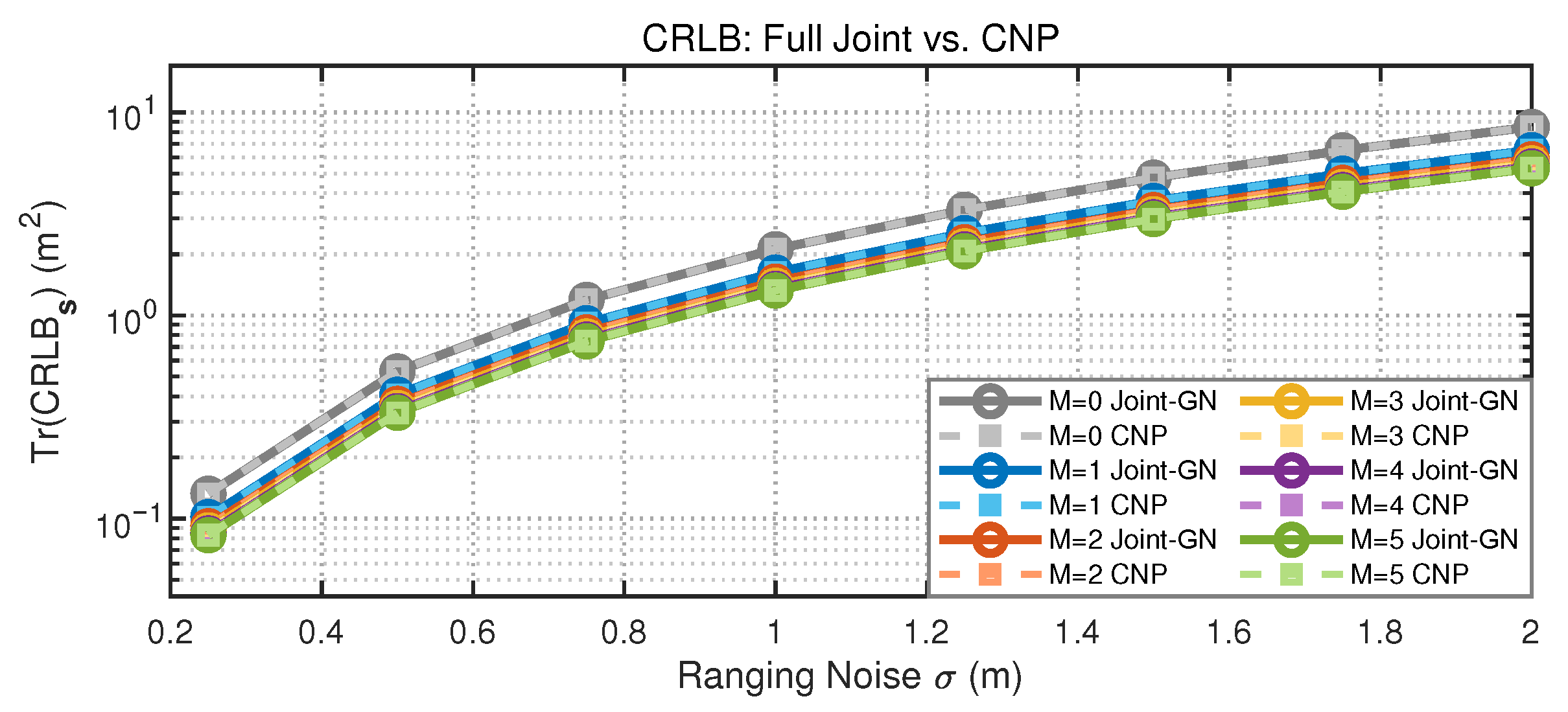
We first examine whether adding NLOS paths improves geometric accuracy, or at least does not degrade it, in accordance with (18). To this end, we compute the trace of the marginal CRLB for the source position, as the number of reflectors M varies from 0 (LOS only) to 5.

As shown in Figure 2, the uncertainty is highest in the LOS-only case. The largest reduction in geometric uncertainty occurs when the first two reflectors are introduced. Additional reflectors continue to reduce the bound, but the improvement becomes smaller because of directional redundancy. The close agreement between the Joint and CNP curves confirms that eliminating clock parameters through the Schur complement preserves the geometric Fisher information.

5.3. Observability Under Geometric Degeneracy

To study sensitivity to trajectory design, we evaluate the condition number $\kappa \left({\mathbf{F}}_{\mathit{\theta }}^{\mathrm{eff}}\right)$ and the minimum eigenvalue ${\lambda }_{\min }$ under two motion patterns:

• Radial Trajectory: The UAV moves directly away from the source, yielding nearly constant LOS bearings.
• Arc Trajectory: The UAV performs a coordinated turn to increase bearing diversity.

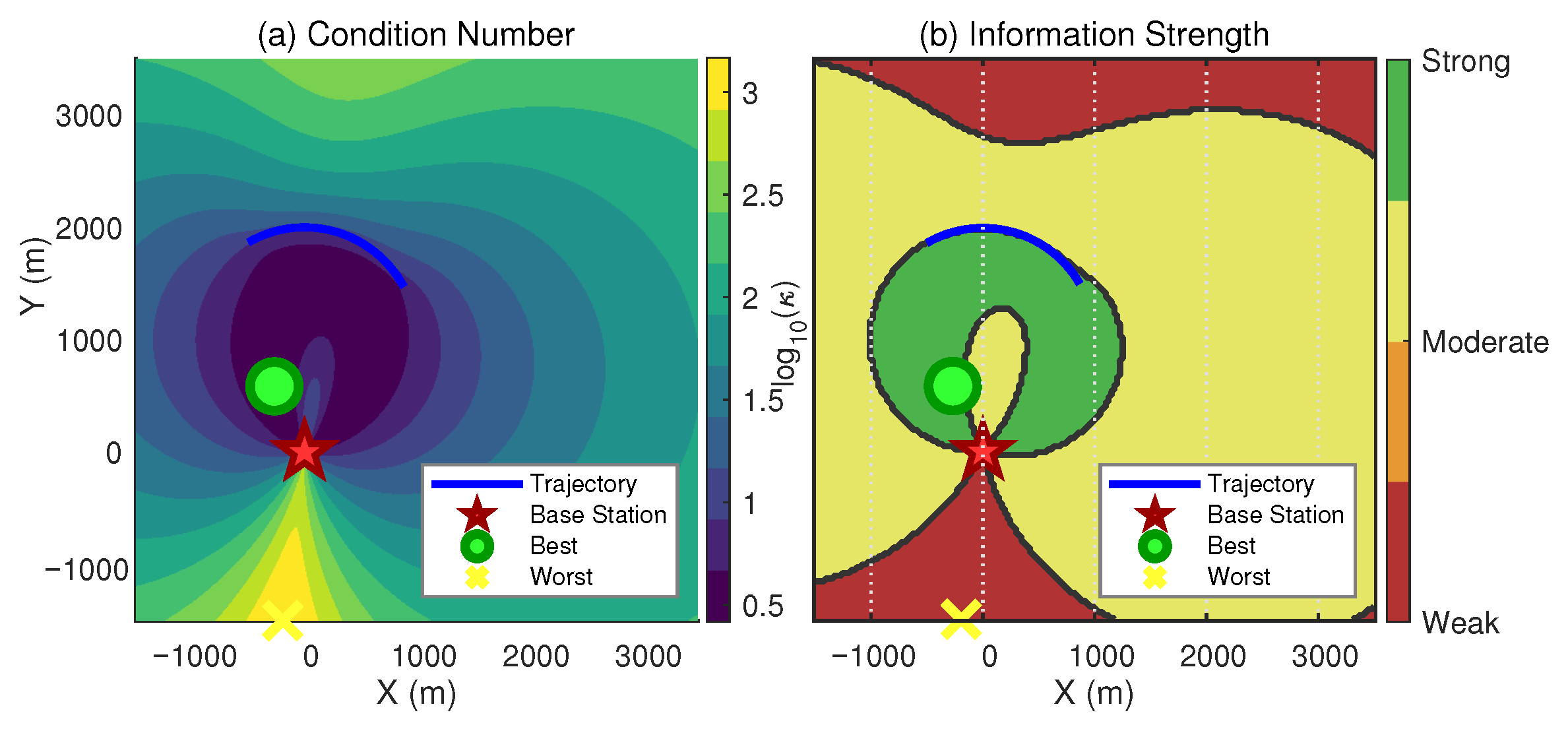
For each motion pattern, spatial observability maps are generated by placing a single NLOS reflector at grid locations and computing the corresponding information metrics.

Analysis of Singularities

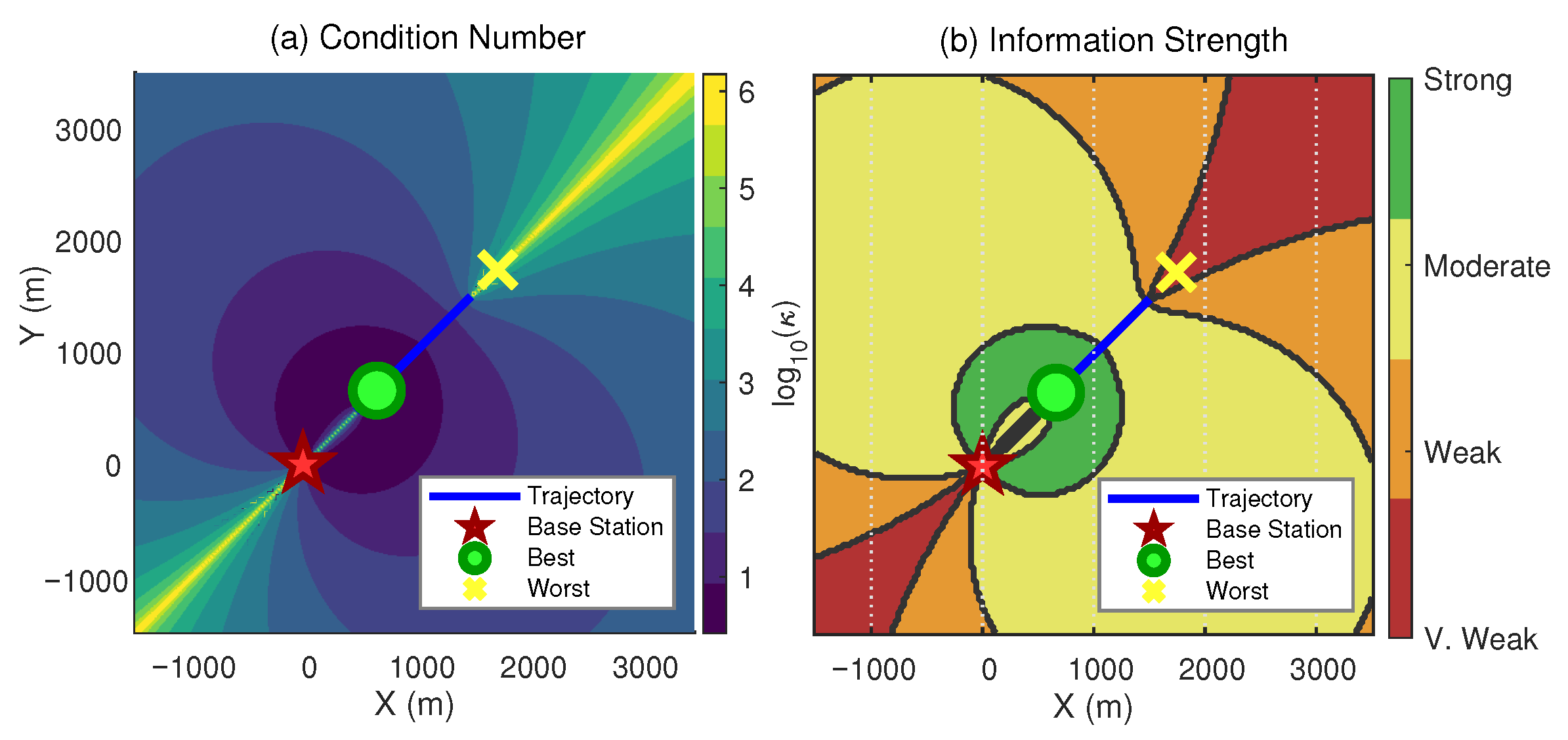
Figure 3 shows that radial motion produces a blind sector in which the reflector becomes nearly collinear with the source–UAV axis, corresponding to ${\varphi }_{k,m}\approx 0$ or $\pi$. In this region, $\kappa \to \infty$, and the reflector position becomes locally unobservable.

By contrast, Figure 4 shows that the arc trajectory greatly reduces the extent of the ill-conditioned region. The changing viewing angle yields a broader area with favorable conditioning.

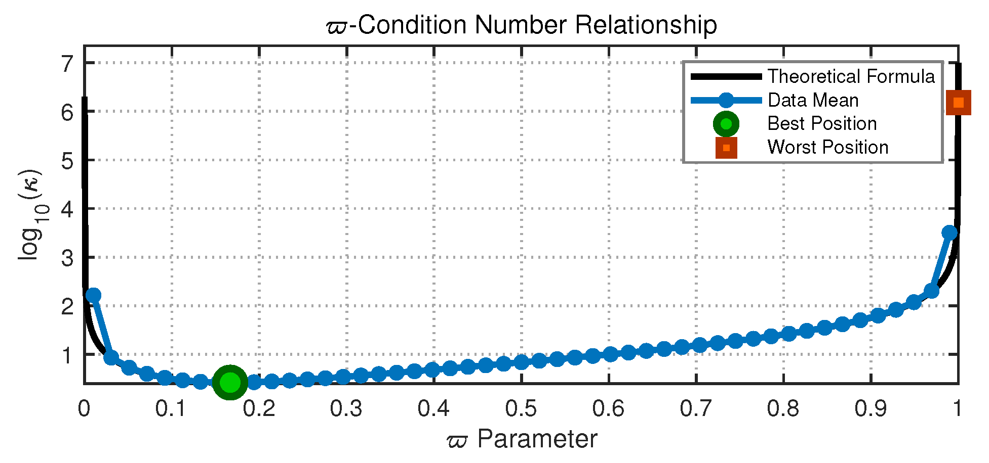
Figure 5 plots the condition number as a function of the angular diversity ratio $\varpi$. The simulated values follow the theoretical curve in (27) closely, with $\kappa$ diverging as $\varpi \to 0$ or 1, and attaining its minimum near $\varpi \approx 0.167$.

These maps can be interpreted as vulnerability maps for autonomous path planning. They show that, although single-bounce geometry is locally observable in theory, robustness depends strongly on maintaining angular diversity. In unknown environments, this motivates maneuvers such as S-turns or orbits that increase $\varpi$ and keep the system away from the identified singular configurations.

5.4. Solver Robustness and Global Convergence

In non-cooperative sensing scenarios where neither the transmitter nor reflector locations are known a priori, the MLE in (12) becomes highly nonconvex. Standard iterative solvers are sensitive to initialization and may converge to poor local minima when the starting point lies outside the basin of attraction of the desired solution.

To evaluate the role and effectiveness of the proposed two-stage framework, we compare it against unseeded iterative solvers, including standard nonlinear least squares and factor-graph optimization, over extensive MC trials.

5.4.1. Experimental Design

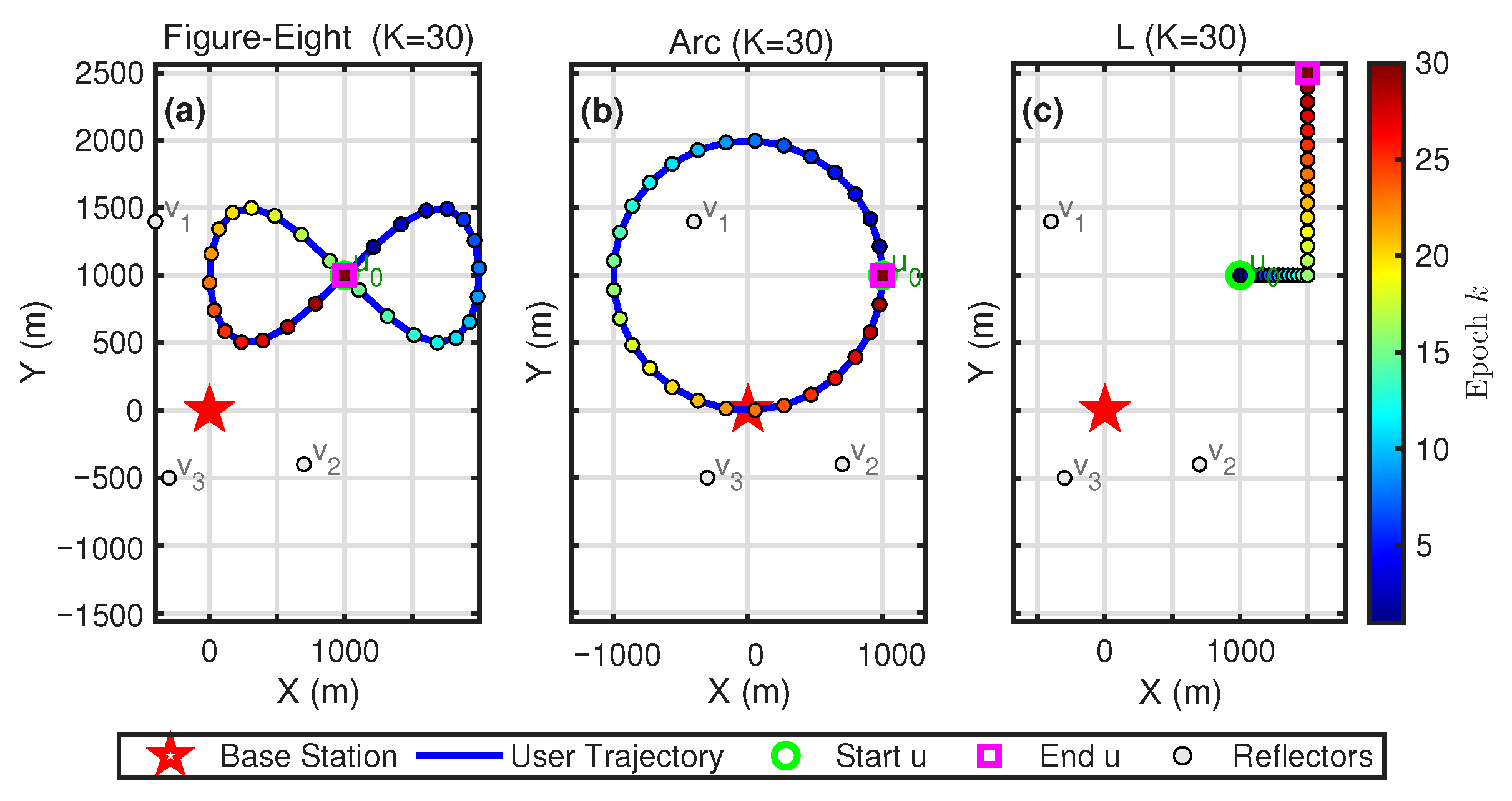
Three UAV trajectories (Figure-Eight, Circular Arc, and L-Shape) are simulated using the reflector layouts in (54). Figure 6 illustrates the corresponding geometry, including the flight paths, initial and final UAV positions, transmitter location, and reflector layout. Each scenario includes $N_{\mathrm{mc}}=1000$ trials with range noise $\sigma =1\mathrm{m}$ and no prior information. Five estimation methods are compared:

• Joint-GN: The standard MLE baseline, solved by Gauss–Newton optimization with random initialization.
• CNP: Stage-II subspace optimization with random initialization after eliminating clock parameters.
• FG (Factor Graph): A graph-based nonlinear least-squares backend widely used in SLAM-related estimation problems.
• CF (Stage I): The proposed closed-form algebraic initializer.
• CF+CNP (Proposed): The complete two-stage method using the algebraic seed followed by CNP-based refinement.

Convergence is declared when $\parallel \widehat{\mathbf{s}}-\mathbf{s}\parallel \le c_{\mathrm{th}}\sqrt{\mathrm{tr}\left({\mathrm{CRLB}}_{\mathbf{s}}\right)},$ with $c_{\mathrm{th}}=40$. This threshold is chosen empirically to account for nonlinear error propagation and finite-sample variability while still distinguishing successful convergence from clearly incorrect solutions.

5.4.2. Convergence Analysis

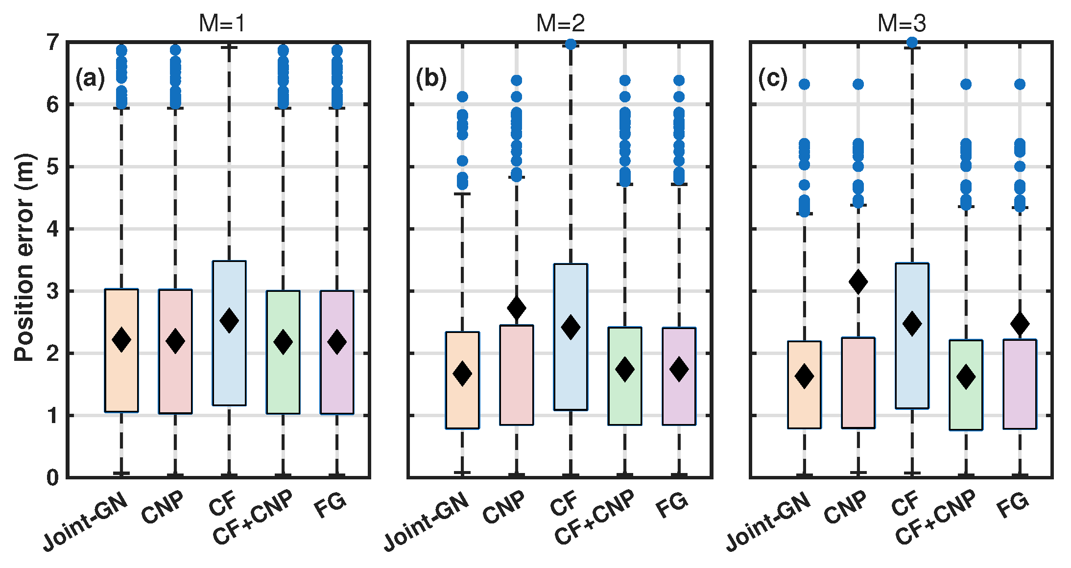
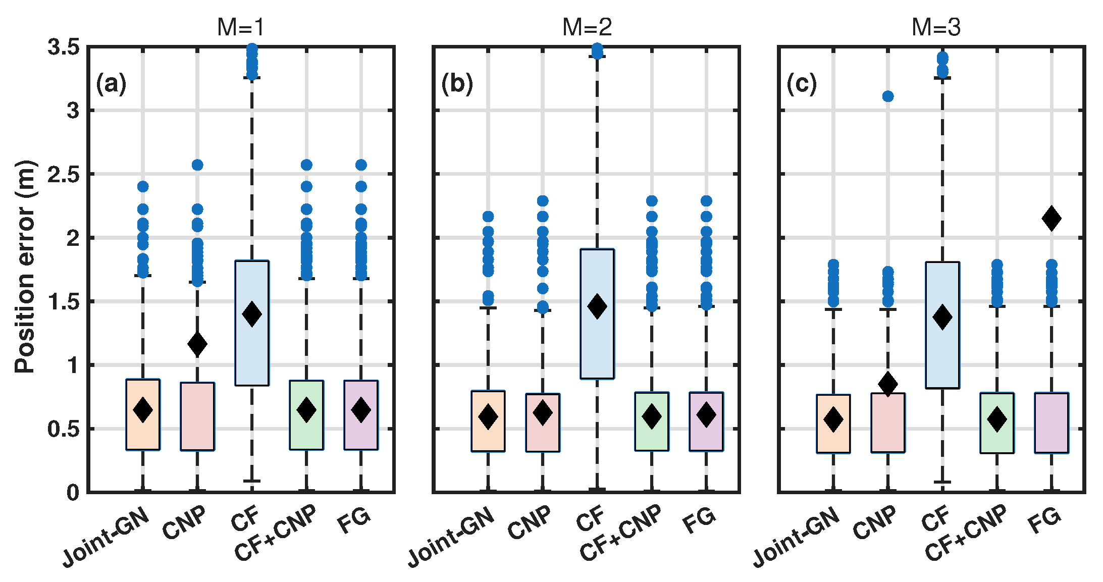
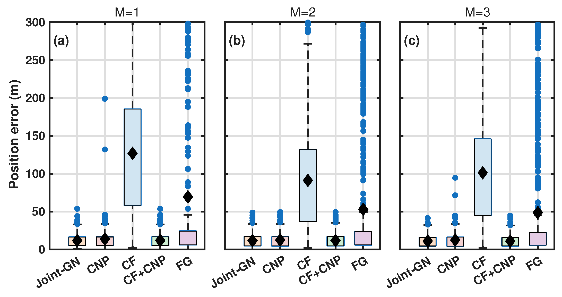
Position error distributions and convergence rates are summarized in

Table 1. Convergence success rate (%) comparison. Best results are shown in bold.

Scenario	Method	$\mathit{M}=1$	$\mathit{M}=2$	$\mathit{M}=3$	Avg.
A: Figure-Eight	Joint-GN	78.9	61.5	57.3	65.9
	CNP	89.5	78.7	73.1	80.4
	FG	99.9	95.5	95.9	97.1
	CF	100.0	100.0	100.0	100.0
	CF+CNP	100.0	100.0	100.0	100.0
B: Circular Arc	Joint-GN	75.3	62.9	60.1	66.1
	CNP	82.6	70.1	64.6	72.4
	FG	100.0	95.9	89.2	95.0
	CF	100.0	100.0	100.0	100.0
	CF+CNP	100.0	100.0	100.0	100.0
C: L-Shape	Joint-GN	64.2	61.6	52.7	59.5
	CNP	64.6	62.9	58.7	62.1
	FG	98.6	97.2	97.0	97.6
	CF	100.0	100.0	100.0	100.0
	CF+CNP	100.0	100.0	81.7	93.9

and in Figure 7, Figure 8 and Figure 9. Figure 7 shows the results for the Figure-Eight trajectory, Figure 8 for the Arc trajectory, and Figure 9 for the L-Shape trajectory. The variation across these motion patterns highlights the importance of angular diversity for the proposed framework.

Impact of Dimensionality and Nonconvexity: For randomly initialized solvers (Joint-GN and CNP-GN), convergence deteriorates as the number of reflectors M increases. Although more NLOS paths improve the CRLB, they also increase the complexity of the likelihood landscape and make poor local minima more likely in blind cold-start settings.

Effect of Clock Elimination: Even with random initialization, CNP-GN consistently outperforms Joint-GN across all scenarios. By removing nuisance clock parameters, CNP reduces the effective optimization dimension and improves the basin of attraction of the desired solution.

Behavior of the Algebraic Initializer: The Stage-I CF estimator converges in all tested configurations. By converting the original nonconvex constraints into a pseudo-linear system through inter-epoch differencing, it avoids iterative initialization issues and provides a meter-level initial estimate in the tested scenarios.

Performance of the Hybrid Framework: Combining both stages, CF+CNP attains a 100% convergence rate in the structurally favorable Figure-Eight and Arc trajectories. The FG baseline also performs strongly, with average convergence rates above 95%. In the more challenging L-Shape case with $M=3$, FG achieves a higher convergence rate than CF+CNP. However, this difference should be interpreted together with the accuracy analysis below, where CF+CNP exhibits substantially fewer large-error outliers.

5.4.3. Estimation Accuracy and Outlier Suppression

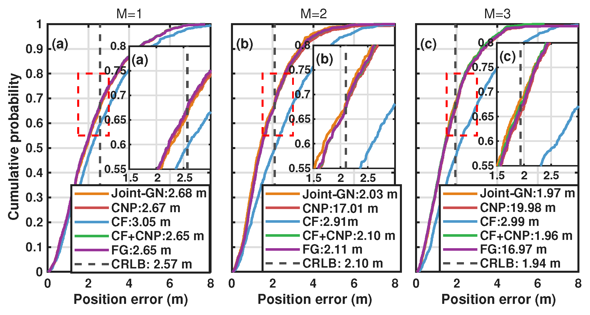
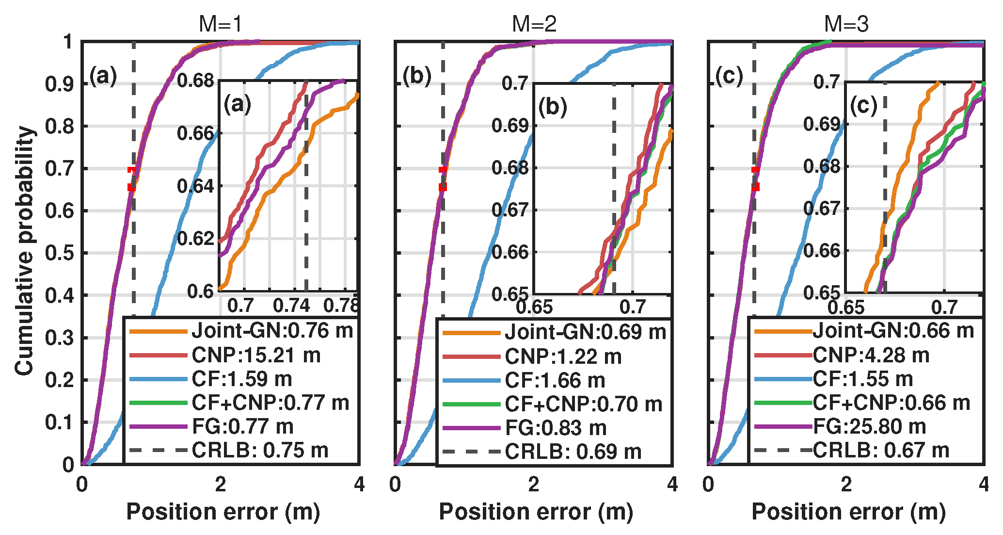
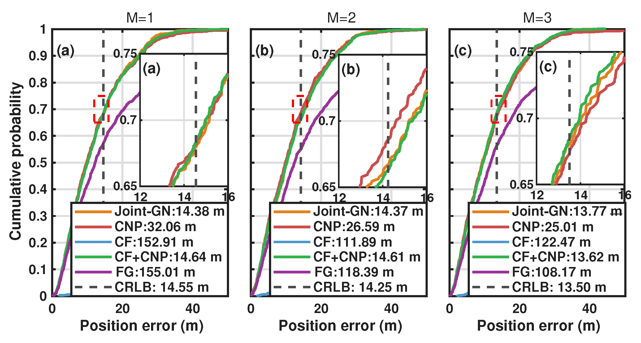
The Cumulative Distribution Functions (CDFs) of the source-position error are shown in Figure 10, Figure 11 and Figure 12. As predicted by the observability analysis in Section 3, the geometric diversity of the UAV trajectory strongly influences accuracy. Among the tested patterns, the Arc trajectory yields the lowest error, followed by the Figure-Eight trajectory and then the L-Shape trajectory. This ordering is consistent with the theoretical result that continuous variation in viewing angle improves conditioning and reduces estimation uncertainty. Stage II refinement is necessary to approach the CRLB, since residual linearization error limits the accuracy of Stage I even though the CF initializer converges in all tested MC trials.

The CDFs also show that the FG baseline exhibits a heavier error tail. For example, in the Circular Arc scenario with $M=3$, CF+CNP tracks the theoretical limit closely with an RMSE of $0.66\mathrm{m}$, while FG exhibits a maximum error of $25.80\mathrm{m}$. In the L-Shape scenario, the maximum FG error increases to $108.17\mathrm{m}$, compared with $13.62\mathrm{m}$ for CF+CNP. These results indicate that, although FG often converges successfully, it remains more vulnerable to large-error outliers in dense multipath settings. By contrast, CF+CNP substantially reduces these outliers through the use of a deterministic algebraic seed.

The benefit of increasing the number of reflectors also saturates beyond a certain point. For instance, in the Arc scenario, increasing M from 1 to 2 reduces RMSE from $0.77\mathrm{m}$ to $0.70\mathrm{m}$, whereas adding further reflectors yields only marginal gains. This suggests that dense reflector mapping is not always necessary to obtain high-precision positioning.

5.4.4. Computational Efficiency Profiling

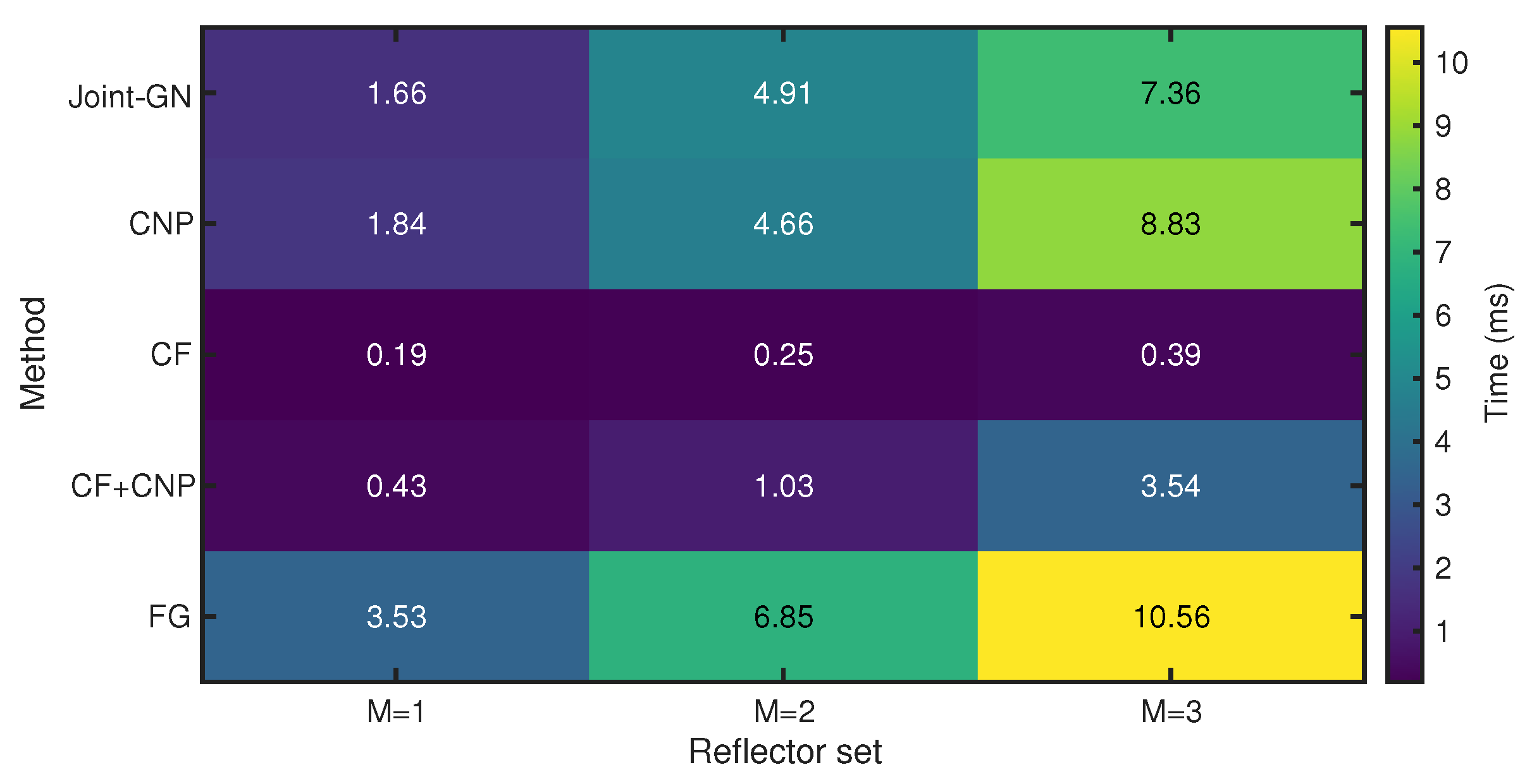
To assess real-time feasibility, all experiments were run in single-thread CPU mode on a standard Intel Core i5-12400F processor using MATLAB R2022b. The average runtime per trajectory is shown in Figure 13.

The CF initializer operates in the sub-millisecond range, requiring only 0.19 to 0.39 ms in the tested scenarios, and exhibits approximately linear scaling with M. This behavior is consistent with the $\mathcal{O}\left(KM\right)$ complexity analysis. It also contrasts with both randomly initialized iterative solvers and the FG baseline. Although FG provides competitive accuracy, its runtime scales less favorably because of graph construction, marginalization, and message-passing overhead, reaching 10.56 ms at $M=3$.

The hybrid CF+CNP pipeline offers a favorable trade-off between computational cost and positioning accuracy. Under the same conditions, it completes the full optimization in 3.54 ms, corresponding to roughly a threefold speedup over FG. Since these results are obtained using single-thread CPU execution without parallelization, they suggest that the proposed framework is suitable for high-rate onboard navigation on embedded UAV platforms under SWaP constraints.

6. Experimental Validation and Analysis

Field experiments in an urban campus environment are used to evaluate the proposed framework under GNSS-denied conditions. Phase I focuses on blind sensing and topology reconstruction from SOP measurements, while Phase II examines dynamic navigation performance along real trajectories.

6.1. Experimental Setup and Signal Pre-Processing

The hardware platform consisted of a Real-Time Kinematic (RTK) GNSS receiver for ground-truth generation and a USRP B210 SDR with an omnidirectional antenna for LTE signal acquisition. The SDR sampling rate was set to 30.72 MHz, which corresponds to the nominal baseband sampling rate of a standard 20 MHz LTE signal (2048-point FFT with 15 kHz subcarrier spacing). Using this nominal rate avoids fractional resampling and preserves the full available bandwidth for high-resolution multipath separation. A blind search detected a commercial LTE downlink at 1815 MHz (Physical Cell ID 333).

To extract TOA measurements in a non-cooperative manner, Cell-Specific Reference Signals (CRSs) were acquired following the method in [32]. LTE TOA estimates were obtained by non-coherent integration over a 200 ms interval. This integration window was selected empirically to balance SNR improvement against motion-induced mismatch. To maintain temporal consistency across heterogeneous data streams, the ground-truth GNSS coordinates were updated at 1 Hz and synchronized through the Pulse Per Second (PPS) signal. The asynchronous GNSS and TOA measurements were then aligned by cubic spline interpolation.

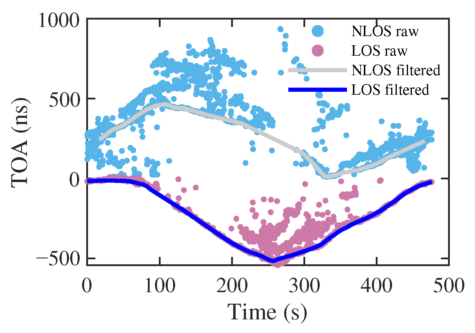
As shown in Figure 14, the received signal contains substantial multipath clutter. ESPRIT was applied to separate the paths in the delay domain. Although the theoretical framework allows multiple reflectors, the experimental estimator was tuned to track only the LOS component and the strongest NLOS component ($M=1$). Practical field measurements showed that secondary and tertiary reflections were substantially attenuated. The resulting increase in ranging variance from these weak components outweighed the limited geometric information they provided. Tracking the strongest NLOS path therefore provided a practical trade-off between geometric diversity and signal reliability. The NLOS outage between $t=210$ s and $t=310$ s was bridged by cubic spline interpolation to preserve measurement continuity.

6.2. Phase I: Inverse Sensing of Environmental Topology

In Phase I, the unknown source and reflector locations were estimated using Random Sample Consensus (RANSAC) on TOA measurements collected over 20 discrete epochs. Reconstruction accuracy was evaluated in a local ENU frame with the origin placed at the initial position. Compared with the ground-truth source position $(-251.40,-135.21)$ m, the estimated source location was $(-257.76,-127.82)$ m, corresponding to an RMSE of 9.75 m. This level of accuracy is consistent with the practical navigation requirements, especially given the use of a 2D model for inherently 3D propagation.

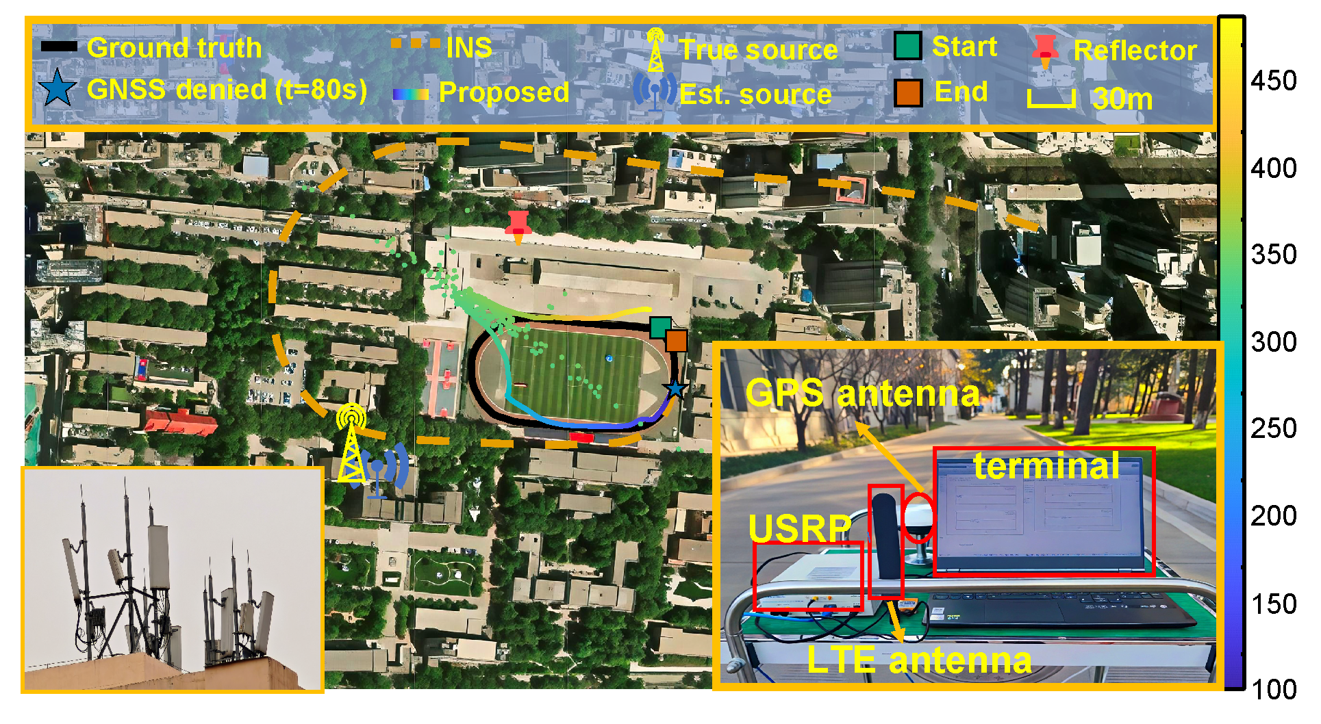
The estimated reflector position at $(-120.36,73.86)$ m is aligned with the stadium boundary wall shown in Figure 15. This agreement suggests that the framework can recover salient environmental geometric structure from non-cooperative RF signals.

6.3. Phase II: Resilient Navigation Assessment

Navigation resilience was evaluated by a semi-physical simulation based on high-dynamic trajectories extracted from real RTK-GNSS data. INS measurements were generated by inverse mechanization of the ground-truth trajectory and corrupted using a realistic Micro-Electromechanical Systems (MEMS) IMU error model. The parameters were selected to match commercial industrial-grade sensors. In particular, the gyroscope constant bias (0.01°/s), gyroscope white noise standard deviation (0.05°/s), accelerometer constant bias ($0.01{\mathrm{m}/\mathrm{s}}^2$), and accelerometer noise floor ($0.001{\mathrm{m}/\mathrm{s}}^2$) were chosen to reflect practical sensor characteristics. Initial alignment errors of 0.05° in heading and $0.01\mathrm{m}/\mathrm{s}$ in velocity were also introduced at the GNSS-denied transition.

To emulate jamming, GNSS signals were interrupted at $t=80\mathrm{s}$, while the preceding interval was used to accumulate observability for the unknown SOP states. During GNSS denial, the position was propagated by trapezoidal integration of the corrupted IMU data.

As shown in Figure 15, the pure INS solution (orange dashed line) accumulates drift rapidly after GNSS denial and deviates substantially from the ground truth by the end of the mission. By contrast, the SOP-aided trajectory remains close to the ground truth throughout the flight. This visual comparison is consistent with the quantitative improvement over pure inertial navigation and indicates that SOP observations can effectively constrain inertial drift in a realistic operating scenario.

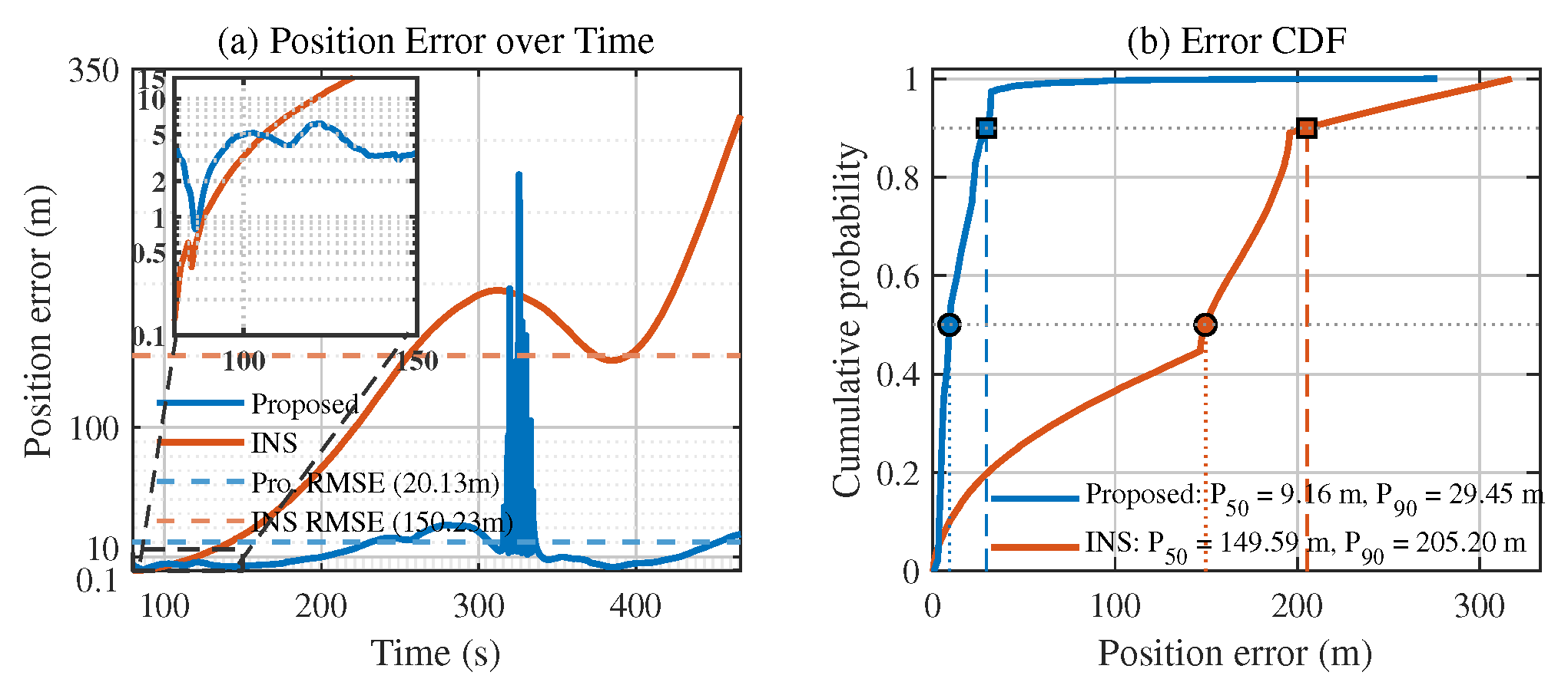
A quantitative evaluation is provided in Figure 16. The proposed method achieves median ($P_{50}$) and 90th-percentile ($P_{90}$) position errors of 9.16 m and 29.45 m, respectively, whereas the pure INS reaches 149.59 m and 205.20 m. Since the LOS and NLOS observations from a single transmitter provide sufficient geometric constraints, the RMSE remains near 5 m during the first 150 s of GNSS denial. The increase in error around $t\approx 320$ s in Figure 16a is attributed to TOA inaccuracies during the NLOS outage. Once reliable geometric constraints are restored, the position error returns to the sub-10-m range.

Although the proposed framework remains stable overall, localized estimation outliers appear as brief deviations in Figure 15. These deviations are primarily caused by temporary loss of the dominant NLOS path in the complex campus environment. Notably, they occur during the NLOS outage, which is consistent with the role of resolvable NLOS multipath as an important geometric constraint in the single-transmitter setting.

Two directions may reduce such deviations in future implementations. First, tighter integration with the INS would allow high-rate inertial constraints to bridge short RF outages more effectively. Second, tracking multiple independent NLOS paths ($M>1$) would provide additional spatial redundancy so that the temporary loss of one reflected component would not severely degrade the available geometry.

Overall, the experimental results show that the framework can achieve meter-level accuracy when valid NLOS components are available. Unlike conventional opportunistic navigation methods that suppress NLOS components to avoid bias [30], and unlike multipath-SLAM methods that rely on cooperative infrastructure or prior maps, the proposed approach uses ambient discrete scatterers to mitigate structural unobservability in a fully non-cooperative setting. In addition, the millisecond-level runtime of the algebraic initializer (cf. Figure 13) supports its use on SWaP-constrained UAV platforms that reuse existing LTE/GNSS antenna hardware.

At the same time, practical deployment must account for several operational assumptions. The discrete scattering model assumes stationary reflectors, such as the stadium boundary wall in Figure 15; highly dynamic environments with moving scatterers would likely require Doppler-based pre-filtering to suppress time-varying bias. Moreover, the linear clock-drift model limits the admissible integration interval, so the UAV should execute angularly diverse maneuvers early enough to accumulate observability before oscillator drift degrades the measurements.

7. Conclusions

This paper treats environmental multipath not only as a source of interference but also as a deterministic geometric constraint for navigation. A hierarchical two-stage solver is developed to address structural unobservability in non-cooperative environments without requiring prior infrastructure maps or synchronized clocks.

The proposed framework is particularly relevant to SWaP-constrained UAV platforms operating in applications such as urban air mobility and disaster response. By reusing existing LTE signals and standard onboard hardware, the method avoids the payload cost associated with active sensors such as LiDAR. As a result, it can provide a lightweight backup navigation modality when GNSS signals are degraded or denied.

References

- Mozaffari, M.; Saad, W.; Bennis, M.; Nam, Y.H.; Debbah, M. A tutorial on UAVs for wireless networks: Applications, challenges, and open problems. IEEE Commun. Surv. Tutorials 2019, 21, 2334–2360. [Google Scholar] [CrossRef]
- Nex, F.; Armenakis, C.; Cramer, M.; Cucci, D.A.; Gerke, M.; Honkavaara, E.; Kukko, A.; Persello, C.; Skaloud, J. UAV in the advent of the twenties: Where we stand and what is next. Isprs J. Photogramm. Remote. Sens. 2022, 184, 215–242. [Google Scholar] [CrossRef]
- Behravan, A.; Yajnanarayana, V.; Keskin, M.F.; Chen, H.; Shrestha, D.; Abrudan, T.E.; Svensson, T.; Schindhelm, K.; Wolfgang, A.; Lindberg, S.; et al. Positioning and Sensing in 6G: Gaps, Challenges, and Opportunities. IEEE Veh. Technol. Mag. 2022, 18, 40–48. [Google Scholar] [CrossRef]
- Ge, Y.; Kaltiokallio, O.; Rastorgueva-Foi, E.; Keskin, M.F.; Chen, H.; Jornod, G.; Talvitie, J.; Valkama, M.; Hofmann, F.; Wymeersch, H. Sensing with Mobile Devices through Radio SLAM: Models, Methods, Opportunities, and Challenges. arXiv 2025, arXiv:2509.07775. [Google Scholar] [CrossRef]
- Zidan, J.; Adegoke, E.I.; Kampert, E.; Birrell, S.A.; Ford, C.R.; Higgins, M.D. GNSS vulnerabilities and existing solutions: A review of the literature. IEEe Access 2020, 9, 153960–153976. [Google Scholar] [CrossRef]
- Novák, A.; Kováčiková, K.; Kandera, B.; Sedláčková, A.N. Global navigation satellite systems signal vulnerabilities in unmanned aerial vehicle operations: Impact of affordable software-defined radio. Drones 2024, 8, 109. [Google Scholar] [CrossRef]
- Sweat, T.; Harrison, W.K.; Rice, M.; Beard, R.W. Low-SWaP GNSS-denied Navigation using LTE Signals of Opportunity. In Proceedings of the 2025 IEEE/ION Position, Location and Navigation Symposium (PLANS), Monterey, CA, USA, 5–8 May 2025; IEEE: Piscataway, NJ, USA, 2025; pp. 960–967. [Google Scholar]
- Ebadi, K.; Bernreiter, L.; Biggie, H.; Catt, G.; Chang, Y.; Chatterjee, A.; Denniston, C.E.; Deschênes, S.P.; Harlow, K.; Khattak, S.; et al. Present and future of slam in extreme environments: The darpa subt challenge. IEEE Trans. Robot. 2023, 40, 936–959. [Google Scholar] [CrossRef]
- Maaref, M.; Kassas, Z. Ground Vehicle Navigation in GNSS-Challenged Environments Using Signals of Opportunity and a Closed-Loop Map-Matching Approach. IEEE Trans. Intell. Transp. Syst. 2020, 21, 2723–2738. [Google Scholar] [CrossRef]
- Neinavaie, M.; Kassas, Z.M. Cognitive Sensing and Navigation With Unknown OFDM Signals With Application to Terrestrial 5G and Starlink LEO Satellites. IEEE J. Sel. Areas Commun. 2024, 42, 146–160. [Google Scholar] [CrossRef]
- del Peral-Rosado, J.A.; Raulefs, R.; López-Salcedo, J.A.; Seco-Granados, G. Survey of cellular mobile radio localization methods: From 1G to 5G. IEEE Commun. Surv. Tutorials 2017, 20, 1124–1148. [Google Scholar] [CrossRef]
- Shamaei, K.; Kassas, Z. Receiver Design and Time of Arrival Estimation for Opportunistic Localization With 5G Signals. IEEE Trans. Wirel. Commun. 2021, 20, 4716–4731. [Google Scholar] [CrossRef]
- Wang, P.; Wang, Y.; Morton, J. Signal Tracking Algorithm With Adaptive Multipath Mitigation and Experimental Results for LTE Positioning Receivers in Urban Environments. IEEE Trans. Aerosp. Electron. Syst. 2022, 58, 2779–2795. [Google Scholar] [CrossRef]
- Gholami, M.R.; Gezici, S.; Strom, E.G. TDOA based positioning in the presence of unknown clock skew. IEEE Trans. Commun. 2013, 61, 2522–2534. [Google Scholar] [CrossRef]
- Li, F.; Jin, T.; Qin, H. Sparse Parameter Assisted Bias-Robust Localization Based on Concave-Convex Programming Without Priors. IEEE Trans. Aerosp. Electron. Syst. 2025, 61, 14276–14291. [Google Scholar] [CrossRef]
- Huang, Y.; Bai, M.; Li, Y.; Zhang, Y.; Chambers, J. An Improved Variational Adaptive Kalman Filter for Cooperative Localization. IEEE Sensors J. 2021, 21, 10775–10786. [Google Scholar] [CrossRef]
- Kassas, Z.M.; Humphreys, T.E. Observability analysis of collaborative opportunistic navigation with pseudorange measurements. IEEE Trans. Intell. Transp. Syst. 2013, 15, 260–273. [Google Scholar] [CrossRef]
- Kassas, Z.M.; Abdallah, A. No GPS no problem: Exploiting cellular OFDM-based signals for accurate navigation. IEEE Trans. Aerosp. Electron. Syst. 2023, 59, 9792–9798. [Google Scholar] [CrossRef]
- Ruan, L.; Li, G.; Dai, W.; Tian, S.; Fan, G.; Wang, J.; Dai, X. Cooperative relative localization for UAV swarm in GNSS-denied environment: A coalition formation game approach. IEEE Internet Things J. 2021, 9, 11560–11577. [Google Scholar] [CrossRef]
- Li, T.; Yu, X.; Lin, Q.; Lv, Y.; Wen, G.; Shi, C. Distributed Cooperative Localization for Unmanned Systems Using UWB/INS Integration in GNSS-Denied Environments. IEEE Trans. Instrum. Meas. 2025, 74, 1–13. [Google Scholar] [CrossRef]
- Li, Y.; Zhang, X.; Li, X.; Chen, Z.; Hu, Y.; Yang, J.; Schmeink, A. Cooperative elliptic positioning through single UAV during GNSS outages. IEEE Trans. Wirel. Commun. 2024, 23, 12749–12764. [Google Scholar] [CrossRef]
- Pei, J.; Wang, G.; Ho, K.; Huang, L. Moving transceivers aided localization of a far-field object. IEEE Trans. Mob. Comput. 2024, 23, 12795–12810. [Google Scholar] [CrossRef]
- Morales, J.J.; Kassas, Z.M. Tightly coupled inertial navigation system with signals of opportunity aiding. IEEE Trans. Aerosp. Electron. Syst. 2021, 57, 1930–1948. [Google Scholar] [CrossRef]
- Shamsian, M.R.; Sadeghi, M.; Behnia, F. Joint TDOA and DOA single site localization in NLOS environment using virtual stations. IEEE Trans. Instrum. Meas. 2023, 73, 1–10. [Google Scholar] [CrossRef]
- Chen, J.; Guo, S.; Luo, H.; Li, N.; Cui, G. Non-line-of-sight multi-target localization algorithm for driver-assistance radar system. IEEE Trans. Veh. Technol. 2022, 72, 5332–5337. [Google Scholar] [CrossRef]
- Liu, H.; Wei, Z.; Wang, X.; Wu, H.; Liu, F.; Li, X.; Feng, Z. Multipath Component-Enhanced Signal Processing for Integrated Sensing and Communication Systems. arXiv 2025, arXiv:2506.07495. [Google Scholar] [CrossRef]
- Chu, X.; Lu, Z.; Gesbert, D.; Wang, L.; Wen, X.; Wu, M.; Li, M. Joint vehicular localization and reflective mapping based on team channel-SLAM. IEEE Trans. Wirel. Commun. 2022, 21, 7957–7974. [Google Scholar] [CrossRef]
- Xu, X.; Peng, A.; Hong, X.; Zhang, Y.; Zhang, X.P. Multistate constraint multipath-assisted positioning and mismatch alleviation. IEEE Internet Things J. 2023, 11, 11271–11286. [Google Scholar] [CrossRef]
- Venus, A.; Leitinger, E.; Tertinek, S.; Meyer, F.; Witrisal, K. Graph-based simultaneous localization and bias tracking. IEEE Trans. Wirel. Commun. 2024, 23, 13141–13158. [Google Scholar] [CrossRef]
- Wang, P.; Morton, Y. Multipath Estimating Delay Lock Loop for LTE Signal TOA Estimation in Indoor and Urban Environments. IEEE Trans. Wirel. Commun. 2020, 19, 5518–5530. [Google Scholar] [CrossRef]
- Li, F.; Jin, T.; Qin, H.; Qu, J. Asynchronous terrestrial signal of opportunity-based self-localization with source location uncertainty: Methods and analysis. IEEE Trans. Aerosp. Electron. Syst. 2024, 60, 3711–3725. [Google Scholar] [CrossRef]
- Zhang, Y.; Ho, D.K.C. Multistatic Localization in the Absence of Transmitter Position. IEEE Trans. Signal Process. 2019, 67, 4745–4760. [Google Scholar] [CrossRef]
Figure 1.
Illustration of the sensing geometry featuring the UAV, unknown transmitter, and scatterers.
Figure 2.
Trace of the source-position CRLB versus the number of NLOS paths (M).
Figure 3.
Observability map for radial motion: (a) condition number ; (b) information strength .
Figure 4.
Observability map for arc motion: (a) condition number ; (b) information strength .
Figure 5.
Numerical validation of the theoretical condition number
versus angular diversity ratio
(cf. (
27)).
Figure 6.
Visualization of the test trajectories: (a) Figure-Eight; (b) Circular Arc; (c) L-Shape.
Figure 7.
Estimation error distribution for the Figure-Eight trajectory: (a) ; (b) ; (c) .
Figure 8.
Estimation error distribution for the Arc trajectory: (a) ; (b) ; (c) .
Figure 9.
Estimation error distribution for the L-Shape trajectory: (a) ; (b) ; (c) .
Figure 10.
Figure-Eight trajectory: CDF of source-position error with CRLB overlay for (a) ; (b) ; (c) . The red square indicates the region magnified in the inset.
Figure 11.
Arc trajectory: CDF of source-position error with CRLB overlay for (a) ; (b) ; (c) . The red square indicates the region magnified in the inset.
Figure 12.
L-Shape trajectory: CDF of source-position error with CRLB overlay for (a) ; (b) ; (c) . The red square indicates the region magnified in the inset.
Figure 13.
Average solver runtime versus reflector count M (aggregated over trajectories).
Figure 14.
Processed LTE TOA observations: filtered raw data distinguish the LOS path (blue) from the NLOS path (gray).
Figure 15.
Field experiment setup and trajectory results. The main map compares the ground truth (black), the drifting INS solution (orange), and the proposed SOP-aided solution (gradient color).
Figure 16.
Navigation performance: (a) position error; (b) error CDF.