Cooperative Rapid Search for Evasive Targets Using Multiple UAVs Based on Graph Theory

Highlights

What are the main findings?

• A unified graph-theoretic framework that integrates the environment, evasive targets, and UAVs, providing a consistent framework for cooperative search.
• Develops a Directional Gradient-based Prediction (DG-Prediction) model that captures target evasion intent by guiding probability diffusion along predicted escape corridors, moving beyond isotropic assumptions.

What are the implications of the main findings?

• Enables effective search against intelligent evasive targets by providing a structured, intention-aware model that significantly improves target capture probability in adversarial scenarios.
• Delivers a practical, computationally efficient system that bridges the gap between discrete decision-making and continuous, kinematically feasible trajectory generation for fixed-wing UAV swarms.

Abstract

Rapid search for evasive targets using multiple Unmanned Aerial Vehicles (UAVs) presents significant challenges, as it requires real-time target-motion prediction, multi-agent coordination, and adherence to kinematic constraints. Existing cooperative search methods often assume non-adversarial target behavior or model target motion independently of UAV actions, which reduces their effectiveness against targets that actively evade based on UAV positions. To address these limitations, this study introduces the Cooperative Rapid Search Algorithm for Evasive Targets (CRS-AET). The proposed framework utilizes graph-theoretic modeling to represent spatial-temporal relationships among UAVs, targets, and environmental grids. A directional gradient-based motion prediction (DG-Prediction) method first estimates probable movement areas of dynamic targets within the graph-structured environment. An improved multi-round auction algorithm with graph-based utility propagation (IMRAA) then optimizes UAV resource allocation. Finally, Dubins-Constrained Trajectory Optimization (DC-RTO) is integrated within a distributed model predictive control (DMPC) scheme to ensure kinematic feasibility. Simulation results across three representative scenarios indicate that CRS-AET enables faster target detection, enhanced area coverage, and more efficient coordination than baseline methods. Hardware-in-the-loop (HIL) experiments further confirm the robustness and practical applicability of the framework in realistic operational environments.

1. Introduction

1.1. Background

Multi-UAV (Unmanned Aerial Vehicle) cooperative search has demonstrated great potential in various fields, including target reconnaissance [1], border patrol [2], disaster relief [3], and wildlife search and rescue [4], with significant application value. Compared to a single UAV system, the multi-UAV cooperative mechanism can significantly improve search efficiency and the success rate of target capture through comprehensive optimization of task allocation and path planning [5,6,7]. Existing studies usually decompose the cooperative search problem into two core sub-problems: (1) UAV task allocation strategies based on the spatial distribution characteristics of targets to maximize the overall system effectiveness [8,9]; (2) The design of UAV trajectory planning algorithms that meet coverage and time constraints, which need to consider both flight dynamics and communication limitations [10,11,12,13,14].

However, current research primarily focuses on scenarios of static or low-speed moving targets or only considers simple cases of randomly moving targets. The fixed coverage mode [15] or the grid-based search strategy [16] can achieve high efficiency in non-adversarial scenarios. However, when targets possess the attribute of intelligent escape, their evasive behaviors, such as active path changes and signal hiding, will significantly weaken the effect of the traditional collaborative search strategy, which is specifically reflected in the increase in target loss probability and the increase in resource consumption.

From a modeling perspective, traditional methods discretize the search environment into grid cells [17] and update target probabilities using mechanisms such as Markov transition matrices [18] or Gaussian diffusion kernels [19]. Although these methods account for proximity between neighboring cells, their adjacency structures are typically static and isotropic. As a result, they do not adaptively capture the highly directional and continuous evasive behaviors of intelligent targets. Additionally, a significant limitation of existing approaches is their reliance on separate mathematical descriptions for environment representation, target prediction, and task allocation. This separation leads to information loss during inter-module data conversion and restricts the consistent use of spatial structures throughout the decision-making pipeline. Graph theory offers a natural framework for unifying the description of spatiotemporal relationships among the environment, targets, and UAVs. By modeling environmental units or agents as nodes and dynamic spatial adjacency or interaction relationships as edges, this approach reformulates the cooperative search problem as a unified dynamic graph optimization problem. This paper focuses on leveraging dynamic graph models to accurately represent the continuous motion patterns of evasive targets and to enable efficient, structurally unified cooperative decision-making.

1.2. Related Work

Coordinating multiple UAVs to search for evasive targets is essential to improve search efficiency and success rates. However, most current prediction models have key limitations. They update probabilities using discrete, independent grid cells, which disrupts spatial correlations and fails to capture the continuous motion and directional strategies of targets. As a result, these models struggle to balance prediction accuracy and computational efficiency in dynamic environments. The following section reviews existing modules in target motion prediction, task allocation, and trajectory planning.

For the uncertainty modeling of target motion, existing studies mainly adopt the following three categories of methods: (1) Stochastic process-based methods, which usually assume uniform transition probabilities between grids but fail to fully account for the impacts of directional motion bias and external disturbances. For instance, S. Pérez-Carabaza et al. [18] developed a probability prediction model using Markov chains and historical data. However, their model relies on fixed transition matrices between adjacent grid cells, which structurally limits its ability to cope with sudden evasive maneuvers. Similarly, Zhen et al. [19] incorporated Gaussian distributions to characterize directional uncertainty, yet their static kernel approach does not account for the continuous, dynamic variation in directional errors during target evasion. (2) Probability diffusion-based methods (e.g., Gaussian error models), which are capable of simulating target drift induced by environmental factors, but mostly adopt isotropic diffusion and thus cannot accurately describe the directional evasive behaviors of intelligent targets. Y. Lun [9] and P. Yao [20] applied probability diffusion models to flow direction estimation in continuous scenarios; however, such methods exhibit poor adaptability to discrete grid environments, and often face a trade-off between accuracy and computational efficiency when dealing with highly maneuverable evasive targets. (3) Game theory and reinforcement learning-based methods, which can model adversarial behaviors, but generally suffer from drawbacks such as high data demand and low online learning efficiency. Moreover, most of these methods do not consider the kinematic constraints of fixed-wing UAVs. Relevant studies [21,22,23] are mostly oriented toward rotary-wing UAVs, lacking targeted handling of the maneuverability limitations of fixed-wing platforms. In summary, most existing prediction models are established on discrete, independent grid representations, and lack effective modeling of spatial correlations and directional evasive behaviors, resulting in a failure to balance accuracy and efficiency in dynamic adversarial environments.

In terms of task allocation strategies, most current methods employ heuristic search strategies driven by information entropy maps, as proposed in [18,24]. UAV swarms following this approach preferentially cover regions of high target probability in sequence, subsequently shifting to the next region upon thorough completion. This serial search mode could lead to two major issues: firstly, swarm intelligence may converge prematurely into local optima, resulting in repetitive coverage and resource wastage; secondly, there can be delayed responses to time-sensitive targets, potentially missing critical capture opportunities [25]. While several dynamic allocation methods have been proposed for strike missions [26,27,28], their performance is dependent on accurate target prior information, making them difficult to directly apply to search scenarios where target distributions are uncertain and dynamically changing. In summary, the current task allocation schemes are decoupled from the underlying environmental representation, and the allocation strategies fail to fully leverage the spatial structural information of the environment. This results in low coordination efficiency and makes it challenging to achieve wide area and balanced target search.

Current trajectory planning methods for fixed-wing UAVs typically address path feasibility [29] and kinematic constraints [30] sequentially, which can result in suboptimal or infeasible solutions in dynamic environments. While the Model Predictive Control (MPC) framework is widely utilized, directly incorporating strict kinematic constraints, such as Dubins paths, and achieving collaborative optimization across multiple UAVs remain significant challenges. Furthermore, there is insufficient integration among the planning, perception, and decision-making layers. Planning algorithms generally function in continuous geometric spaces, whereas perception and decision-making are primarily executed on discrete grids. The conversion between these heterogeneous models results in information loss and reduced computational efficiency.

Our prior work proposed the CHTS-CC framework, which effectively addresses the cooperative search problem for moving targets under constrained communications [31]. However, that study exhibits notable limitations: it operates under the core assumption that targets exhibit only routine motion patterns, failing to consider active evasion strategies driven by intelligent decision-making. Furthermore, it relies on a traditional discrete grid-based representation for environmental modeling, which does not fully exploit spatial correlations to support search decision-making. Consequently, its applicability in dynamic, adversarial scenarios remains limited.

In summary, current research faces the predicaments of inaccurate prediction, uncoordinated allocation, and indirect planning when addressing evasive targets. The underlying cause lies in the lack of a unified, continuous, and structured mathematical description for the interactive relationships among the environment, targets, and UAVs. Graph theory offers a promising approach to solving this problem, yet constructing an integrated graph optimization framework that incorporates prediction, allocation, and planning remains a crucial challenge.

1.3. Contributions and Organization

To address the unique demands of large-scale area, intelligent target search missions, we propose a novel Cooperative Rapid Search Algorithm for Evasive Targets (CRS-AET). Different from existing works, the core of this framework lies in establishing a unified graph-theoretic modeling and optimization framework, which integrates the environment, targets, and UAVs into a single spatiotemporal interaction graph for collaborative reasoning and decision-making. The main contributions of this paper are summarized as follows:

(1)

We introduce a graph-theoretic modeling framework that integrates the search environment, dynamic targets, and UAVs within a unified spatiotemporal graph. In this framework, nodes encode multi-dimensional states and edges represent spatial adjacency and interactions, thereby providing a consistent mathematical foundation for prediction, allocation, and planning.

(2)

We introduce the Directional Gradient-based Prediction model (DG-Prediction) for target motion forecasting. This approach incorporates a directional kernel into the graph heat-diffusion equation, guiding probability propagation along predicted evasion corridors. As a result, the model produces a smooth, intention-aware probability distribution, which contrasts with the outcomes of traditional isotropic diffusion.

(3)

We develop an Improved Multi-Round Auction Algorithm (IMRAA) for task allocation. Based on the graph model, this algorithm utilizes a utility function that balances distance incentives, load, and clustering penalties. A graph-propagation mechanism diffuses utility information between UAVs and target nodes, facilitating implicit coordination.

(4)

We propose a real-time path planning scheme, Dubins-Constrained Trajectory Optimization (DC-RTO), that embeds Dubins path constraints directly into a Dynamic Model Predictive Control (DMPC) framework. This integration enables the direct generation of kinematically feasible trajectories for UAVs.

The rest of the paper is organized as follows. Section 2 establishes the models of UAV platforms, target motion, and environmental information, and formalizes the search problem. Section 3 describes the search strategy, which combines DG-Prediction, IMRAA and trajectory planning. Section 4 verifies the effectiveness of the proposed algorithm through multiple sets of simulation experiments. Section 5 summarizes the full paper and prospects future work.

2. Problem Formulation and Models

This section describes the modeling process of the multi-UAV cooperative search from three aspects: simplified UAV model, target motion model, and environmental information model. It also defines the search problem.

2.1. Scenario Description of Multi-UAV Cooperative Search

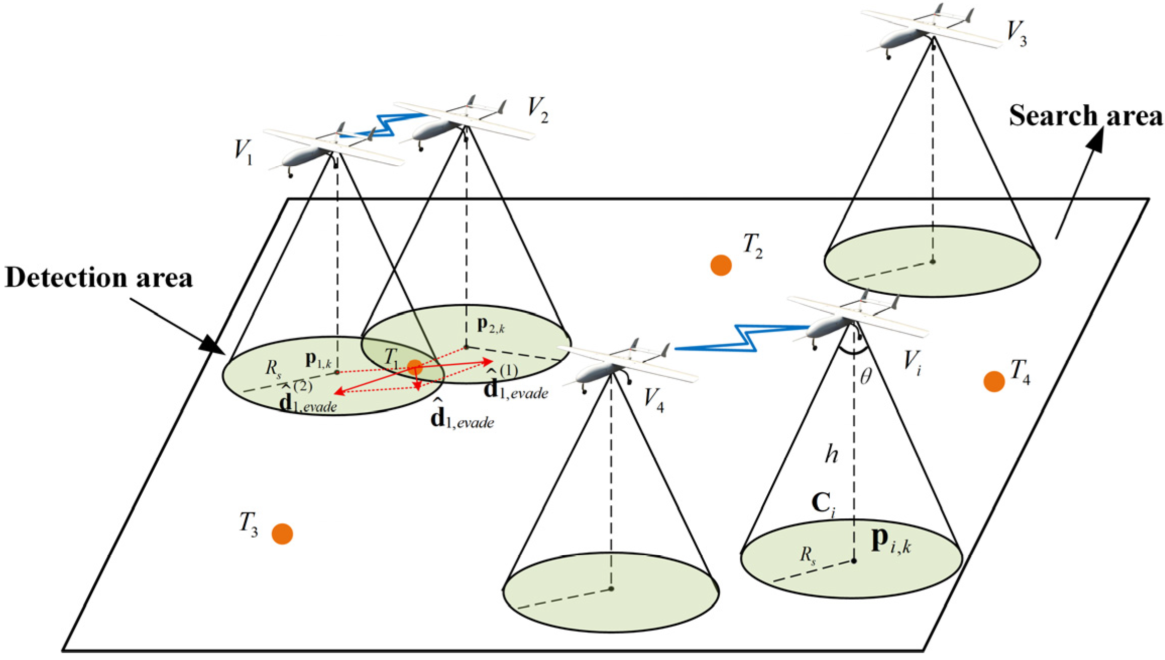
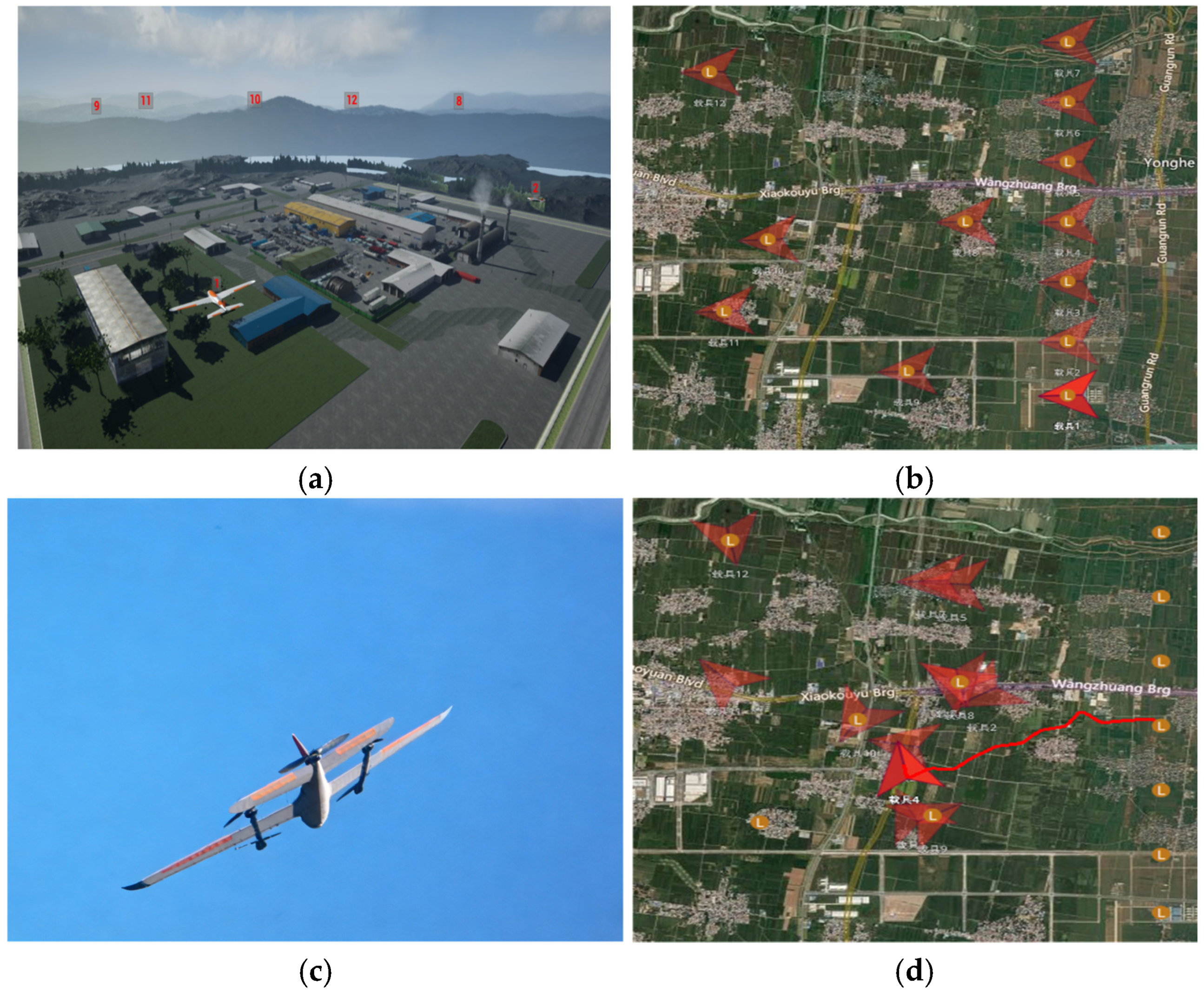
This paper addresses the problem of cooperative multi-UAV target search in complex environments. Figure 1 shows a typical cooperative target search scenario using multiple UAVs. Specifically, $V=\{V_i,i=1,2,3,\dots ,N_v\}$ denotes a set of $N_v$ homogeneous UAVs in the search area and $V_i$ denotes the i-th UAV. $T=\{T_j,j=1,2,3,\dots ,N_t\}$ denotes a set of $N_t$ targets in the search area and $T_j$ denotes the j-th target. Similar to [18], we consider the scenario that the UAV cluster flies at the same altitude, and the flying altitude is high enough so that local terrain fluctuations do not significantly affect the perception range. The proposed algorithm in this paper focuses on a two-dimensional planar task, where $p_{i,k}\in {ℝ}^2$ represents the position of $V_i$ projected onto the 2D plane at time $k$. Constrained by communication constraints, the multi-UAV system performs information exchange via local perception. The primary objective is to optimize UAV flight trajectories for efficient capture of dynamic evasive targets with minimal resource consumption. To strike a balance between model fidelity and computational efficiency, this work focuses on the horizontal coordination of UAVs, assuming that targets move on a 2D plane and UAVs maintain a constant operating altitude. Accordingly, the Z-coordinate is neglected in the graph modeling framework, so as to prioritize real-time trajectory optimization and multi-agent task allocation. Furthermore, as illustrated in Figure 1, the target $T_1$ perceives the sensing intensity from $V_1$ and $V_2$. Individual repulsion vectors ${\widehat{d}}_{1,evade}^{(1)}$ and ${\widehat{d}}_{1,evade}^{(2)}$ are generated in the opposite directions of the UAVs. The final evasion vector ${\widehat{d}}_{1,evade}$ is defined as the normalized resultant vector, which directs the target toward the safest region with the lowest sensing gradient. A detailed description is provided in Section 2.3 to clarify the physical interpretation of this vector.

2.2. Simplified UAV Model

This paper addresses a small fixed-wing UAV with constant speed and fixed altitude cruise. The UAV flies forward at a fixed speed $v_u$ and is limited by the maximum yaw angle. The position of $V_i$ at time k is $p_{i,k}=(x_{u,i}(k),y_{u,i}(k))$. The motion model of $V_i$ is expressed as follows:

$$\left[\begin{array}{c}{x}_{u,i}(k+1)\\ y_{u,i}(k+1)\\ {\psi }_i(k+1)\end{array}\right]=\left[\begin{array}{c}{x}_{u,i}(k)\\ y_{u,i}(k)\\ {\psi }_i(k)\end{array}\right]+\left[\begin{array}{c}{v}_{u,i}\mathrm{\Delta }t\cos {\psi }_i(k)\\ v_{u,i}\mathrm{\Delta }t\sin {\psi }_i(k)\\ \mathrm{\Delta }{\psi }_i(k)\end{array}\right]$$

(1)

where $v_u$ is the flight rate of $V_i$. $\mathrm{\Delta }t$ is the time interval from time k to time k + 1. ${\psi }_i(k)$ is the yaw angle of $V_i$, $\mathrm{\Delta }{\psi }_i(k)\in \left[-\mathrm{\Delta }{\psi }_{\max },\mathrm{\Delta }{\psi }_{\max }\right]$ is the change in yaw angle, and $\mathrm{\Delta }{\psi }_{\max }$ is the maximum yaw angle of the UAV.

This paper focuses on small fixed-wing UAVs equipped with sensors. When the sensors carried by the UAVs are horizontally stable to eliminate interference caused by the UAV’s motion, and the flight altitude $h$ is much greater than local terrain undulation $\mathrm{\Delta }z$, $h\gg \mathrm{\Delta }z$, the oblique-cone field of view can be safely projected onto the horizontal reference plane as a circular footprint with radius $R_s=h·\tan (\theta /2)$, where $\theta$ is the angular field of view of the sensor [32]. As shown in Figure 1, under this assumption, the original oblique cone field of view can be simplified to a two-dimensional circular coverage area. During the search process, a single UAV independently performs search detection on the area within its sensor coverage with its sensing range $C_i=\left\{g_m\right|‖g_m-p_{i,k}‖\le R_s\}$.

2.3. Target Motion Model

In this paper, the structure and motion attitude of the target is considered to be a prime, disregarding UAV movement along the Z-axis. The target’s position at time $k$ is $\left(x_t(k),y_t(k)\right)$. We assume the target moves along its planned route when unaware of UAV presence and changes heading to evade upon detection. This approximates an intelligent evasion scenario. Then, the motion model for $T_j$ is expressed as follows:

$$\left[\begin{array}{c}{x}_{t,j}(k+1)\\ y_{t,j}(k+1)\\ {\varphi }_j(k+1)\end{array}\right]=\left[\begin{array}{c}{x}_{t,j}(k)\\ y_{t,j}(k)\\ {\varphi }_j(k)\end{array}\right]+\left[\begin{array}{c}{v}_{t,j}(k)\mathrm{\Delta }t\cos {\varphi }_j(k)\\ v_{t,j}(k)\mathrm{\Delta }t\sin {\varphi }_j(k)\\ \mathrm{\Delta }{\varphi }_j(k)\end{array}\right]$$

(2)

$$p_{j,k+1}^t=p_{j,k}^t+v_{t,j}(k)·\mathrm{\Delta }t·\widehat{d}$$

(3)

where $p_{j,k}^t=(x_j^t(k),y_j^t(k))$ is the position of $T_j$ at time $k$, and $p_{j,k+1}^t$ is the position of $T_j$ at the next time $k+1$. ${\varphi }_j(k)$ is the movement direction of $T_j$. $\mathrm{\Delta }{\varphi }_j(k)$ is the heading angle of $T_j$. $v_j^t(k)$ is the velocity of $T_j$ at time $k$. $\widehat{d}$ is the current direction of the target’s motion in unit vector.

For dynamic targets with reconnaissance-avoidance characteristics, the actual target is assumed to possess anti-reconnaissance capabilities, enabling it to sense the presence of nearby UAVs. When the UAV enters its sensing range, $R_s<‖p_{i,k}-p_{j,k}^t‖\le R_t$, the target $T_j$ initiates evasive maneuvers, where $R_s$ denotes the perception range of UAV $V_i$, $R_t$ denotes the perception range of target $T_j$. Upon sensing the UAV, the target adjusts its movement direction away from the UAV’s path. The target’s position is updated along the evasive path, and the new equation of motion is as follows:

$$p_{j,k+1}^t=p_{j,k}^t+v_j^t(k)·\mathrm{\Delta }t·{\widehat{d}}_{j,evade}$$

(4)

where ${\widehat{d}}_{j,evade}$ is the unit vector of the evasion direction relative to multiple UAVs. In this paper, the evasion direction is determined based on the relative position between $T_j$ and $V_i$ with $r_{j,i}^k=p_{j,k}^t-p_{i,k}$. In order to move away from the UAV, the target will move in the opposite direction of the position. ${\widehat{d}}_{j,evade}^{(i)}$ is the unit vector of the avoidance direction relative to a single $V_i$:

$${\widehat{d}}_{j,evade}^{(i)}=-{\displaystyle \frac{r_{j,i}^k}{‖r_{j,i}^k‖}}=-{\displaystyle \frac{p_{j,k}^t-p_{i,k}}{‖p_{j,k}^t-p_{i,k}‖}}$$

(5)

Assume the presence of multiple UAVs, where the target executes combined avoidance maneuvers based on the positions of all UAVs. The positional influences of all UAVs are averaged using ${\widehat{d}}_{j,evade}=-{\displaystyle \sum _{i=1}^{N_v^c}{w}_i}·{\widehat{d}}_{j,evade}^{(i)}$, where ${\mathcal{U}}_{t,j}^k$ is the set of all UAVs within the sensing range of $T_j$. The avoidance strength $w_i$ is defined by $w_i=1/\left|r_{j,i}^k\right|, i\in {\mathcal{U}}_{t,j}^k$, with strength increasing as the UAV approaches the avoidance direction. The evasion direction is shown below:

$${\widehat{d}}_{j,evade}=-{\displaystyle \sum _{i=1}^{\left|{\mathcal{U}}_{t,j}^k\right|}\frac{r_{j,i}^k}{{‖r_{j,i}^k‖}^2}}=-{\displaystyle \sum _{i=1}^{\left|{\mathcal{U}}_{t,j}^k\right|}\frac{(x_j^t-x_{u,i},y_j^t-y_{u,i})}{{(x_j^t-x_{u,i})}^2+{(y_j^t-y_{u,i})}^2}}$$

(6)

It is crucial to emphasize that this motion model merely defines the ground-truth adversarial environment. From the UAVs’ perspective, they possess no prior knowledge of the targets’ exact coordinates, movement rules, or specific evasion policies, and must rely on an environmental information map to infer their whereabouts under strictly asymmetric information.

2.4. Environmental Information Map Modeling

In this paper, the rectangular task area of $L_x\times L_y$ is rasterized and divided into $M=N_x\times N_y$ discrete raster cells of $\mathrm{\Delta }x\times \mathrm{\Delta }y$, task area $\Omega =\left\{1,\dots ,M\right\}$. To facilitate vectorized matrix operations in the subsequent graph-based algorithms, the 2D spatial grid is mathematically flattened into a 1D array with cell indices $m\in \{1,\dots ,M\}$. The translation between the 2D grid coordinates $(n_x,n_y)$ and the 1D index $m$ is defined using standard row-major ordering as $m=(n_y-1)N_x+n_x$. The center point of the $m$-th grid cell is used to represent its continuous physical location, denoted by the 2D coordinate vector $g_m=(x_m,y_m)$. Based on the discrete grid indices $(n_x,n_y)$ and the cell resolutions $\mathrm{\Delta }x$, $\mathrm{\Delta }y$, the physical center coordinates are mapped as $x_m=(n_x-0.5)\mathrm{\Delta }x$ and $y_m=(n_y-0.5)\mathrm{\Delta }y$ Here, $N_x=L_x/\mathrm{\Delta }x$, $N_y=L_y/\mathrm{\Delta }y$ denote the total number of grids along the horizontal and vertical axes, respectively.

2.4.1. Initialization of Target Prior Probability Map

The target probability distribution graph $p_m^i(k)\in [0,1]$ indicates the target existence probability estimate of grid $g_m$ by UAV $V_i$ at time k. Through fully utilizing detected environmental information to update the probability map, target distribution can be better predicted, enabling more effective target search in time-varying environments. In practical applications, the initial probability distribution of the target $p_m^i(0)$ can be constructed based on the availability of prior information from satellite data, sensor networks, historical records, or intelligence sources. When there is no prior information about the target location, the search area is typically discretized into a grid and assigned a uniform probability distribution. If positional prior information is available, the distribution is instead represented using a Gaussian model centered on the estimated location. Furthermore, when motion-related priors such as the target’s velocity and heading are known, the initial distribution $p^i(0)={\left[p_1^i(0),p_2^i(0),\dots ,p_M^i(0)\right]}^T\in {ℝ}^M$ will be further refined as a Gaussian distribution with the target’s estimated position $p_{j,k}^t$ and the uncertainty in the target’s position ${\delta }_0^2$ [19].

2.4.2. Sensor Observation Update

After obtaining the initial probability distribution $p^i(0)$, the UAV system performs two-dimensional probability evolution at moment $k$ as the search mission progresses: target dynamic state transition and sensor observation update.

For the target dynamic state transition process, this paper will detail in Section 3.2 to obtain the prior probability of the prediction $p_{s,m}^i(k)$ output of the graph-enhanced probability diffusion module. For the sensor observation update process, it is assumed that the UAV reaches a predefined grid node $g_m$ at moment $k$ and performs detection, with its sensor detection probability $p_d\in [0,1]$ and its sensor false alarm probability $p_f\in [0,1]$. Combined with the actual detection result $b_m^i(k)$, the UAV uses the Bayesian criterion [33] to correct the prior prediction probability $p_{s,m}^i(k)$ for observation, thereby obtaining the final posterior probability $p_m^i(k)$ of target existence at time $k$. The specific description is as follows:

$$p_m^i(k)=\left\{\begin{array}{ll}{p}_{s,m}^i(k)+{\displaystyle \frac{\left(p_d-p_f\right)(1-p_{s,m}^i(k))p_{s,m}^i(k)}{p_d{p}_{s,m}^i(k)+p_f(1-p_{s,m}^i(k))}},\hfill & b_m^i(k)=1\hfill \\ p_{s,m}^i(k)+{\displaystyle \frac{\left(p_f-p_d\right)(1-p_{s,m}^i(k))p_{s,m}^i(k)}{\left(1-p_d\right)p_{s,m}^i(k)+\left(1-p_f\right)(1-p_{s,m}^i(k))}},\hfill & b_m^i(k)=0\hfill \end{array}\right.$$

(7)

where $b_m^i(k)=1$ indicates that the target is detected by $V_i$ at time k in grid $g_m$, and $b_m^i(k)=0$ indicates that the target is not detected. The updated probability map is $p^i(k)={\left[p_1^i(k),p_2^i(k),\dots ,p_{s,M}^i(k)\right]}^T\in {ℝ}^M$.

2.4.3. Environment Uncertainty Map Update

In this paper, uncertainty ${\chi }_m^i(k)$ is employed to characterize the UAV $V_i$’s perception of the environmental grid $g_m$ at time k. At the outset, the environmental uncertainty is quantified as the information entropy associated with the initial target existence probabilities across the search grid.

$${\chi }_m^i(0)=-p_m^i(0){\log }_2{p}_m^i(0)-(1-p_m^i(0))·{\log }_2(1-p_m^i(0))$$

(8)

Here, each grid cell is assumed to have an identical likelihood of containing the target at the initial stage $p_m^i(0)=1/2$. As multiple UAVs collaboratively explore the area, their accumulated observations progressively enhance knowledge of the environment, leading to a continuous reduction in uncertainty [12].

$${\chi }_m^i(k+1)=\left\{\begin{array}{cc}\eta ·{\chi }_m^i(k)& g_m\in C_i \\ (1-\eta )·{\chi }_m^i(k)& g_m\notin C_i \end{array}\right.$$

(9)

where the uncertainty ${\chi }_m^i(k)$ of a grid cell decreases sharply when it is within the sensor coverage $C_i$, while it maintains a marginal reduction when outside $C_i$, reflecting the variation in environmental uncertainty as the search proceeds in greater depth. $\eta$ is the decay factor of information uncertainty in the environment. This paper sets $\eta =0.02$.

2.5. Problem Formulation

When multiple UAVs perform search tasks, their motion states can be uniformly represented in a common state space, allowing the multiple UAVs participating in the task to be regarded as a multi-input, multi-output cooperative control system. At the time $k$, the state of the system is recorded as $x(k)=\{x_1(k),x_2(k),\dots ,x_{N_v}(k)\}$, and the corresponding control input is $u(k)=\{u_1(k),u_2(k),\dots ,u_{N_v}(k)\}$. The state transition equation of the system can be described as $x(k+1|k)=f(x(k),u(k))$, where $f\left(·\right)$ is the state transition function. According to (1), the state of the UAV $V_i$ at time k is $x_i(k)={[p_{i,k},{\psi }_i(k)]}^T$, with control input $u_i(k)=\mathrm{\Delta }{\psi }_i(k)$. $\mathrm{\Delta }{\psi }_i(k)$ is selected as the optimization decision variable. To evaluate the overall effectiveness of multi-UAV cooperative search, we introduced the UAV search effectiveness function $J^k(x(k),u(k))$. The search effectiveness function is a multi-objective function that comprehensively considers the benefits and costs of multiple UAVs in the search process, as follows:

(1)

Regional Target Discovery Benefits: It is expressed as the cumulative sum of the target existence probability within ${\Omega }_i={\cup }_i{\mathrm{C}}_i(k)$, the union of all grid cells covered by the UAV $V_i$. $J_T$ is defined as follows:

$$J_T(k)={\displaystyle \sum _{i=1}^{N_v}{\displaystyle \sum _{m\in {\Omega }_i}(1-{\xi }_m^i(k))p_m^i(k)}},$$

(10)

where ${\xi }_m^i(k)$ represents whether a target is confirmed to exist in grid $g_m$. If $p_m^i(k)\ge {\delta }_p$, ${\xi }_m^i(k)=1$; otherwise, ${\xi }_m^i(k)=0$. ${\delta }_p$ is the predefined existence probability threshold; this paper sets ${\delta }_p=0.9$. Once $p_m^i(k)$ reaches ${\delta }_p$, the discovery benefit for this grid drops to zero, incentivizing the UAV to search elsewhere.

(2)

Multi-UAV Expected Detection Benefits: $J_F$ forces the UAVs to prioritize exploring highly probable but currently highly uncertain regions. $J_F$ is defined as follows:

$$J_F(k)={\displaystyle \sum _{i=1}^{N_v}{\displaystyle \sum _{m\in {\Omega }_i}{\chi }_m^i(k)·p_m^i(k)}}$$

(11)

(3)

Implementation Costs: To minimize UAV turns and flight distances during the search process, the UAV is guided to complete the task with the lowest execution cost, which is expressed here by the change of UAV yaw angle. N is the control time domain of DMPC. The cost of implementation of the task at time k is defined as:

$$C_1(k)={\displaystyle \sum _{i=1}^{N_v}{\displaystyle \sum _{k=1}^N\left|{\psi }_i(k)-{\psi }_i(k-1)\right|}}$$

(12)

(4)

Collision Avoidance Costs: To avoid the collision between UAVs in the process of coordinated search, virtual repulsion is introduced to construct the UAV inter-copter collision prevention mechanism, and $V_i$ is repelled by the repulsive force generated by other UAVs at time k as:

$$\left\{\begin{array}{l}{F}_{ij}=\left\{\begin{array}{l}{k}_f{e}^{-{\omega }_f{D}_{ij}{E}_{ij}},D_{ij}⩽D_{safe},\left|{\phi }_{ij}\right|⩽{\phi }_{\max }\hfill \\ 0,\mathrm{otherswise}.\hfill \end{array}\right.\hfill \\ F_i(k)={\displaystyle \sum _{j=1,i\ne j}^{N_v}{F}_{ij}(k)}\hfill \\ C_2(k)=e^{|F_i(k)|\sin ({\theta }_{uF}(k+1|k))}\hfill \end{array}\right.$$

(13)

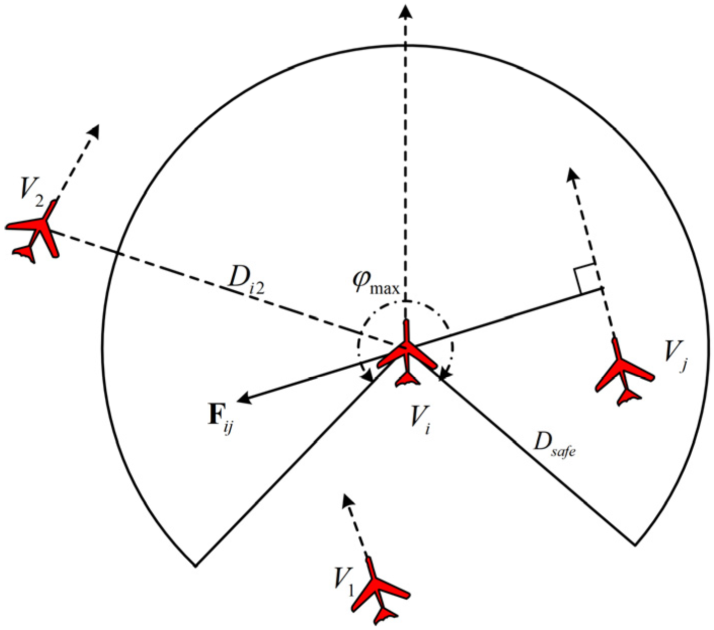
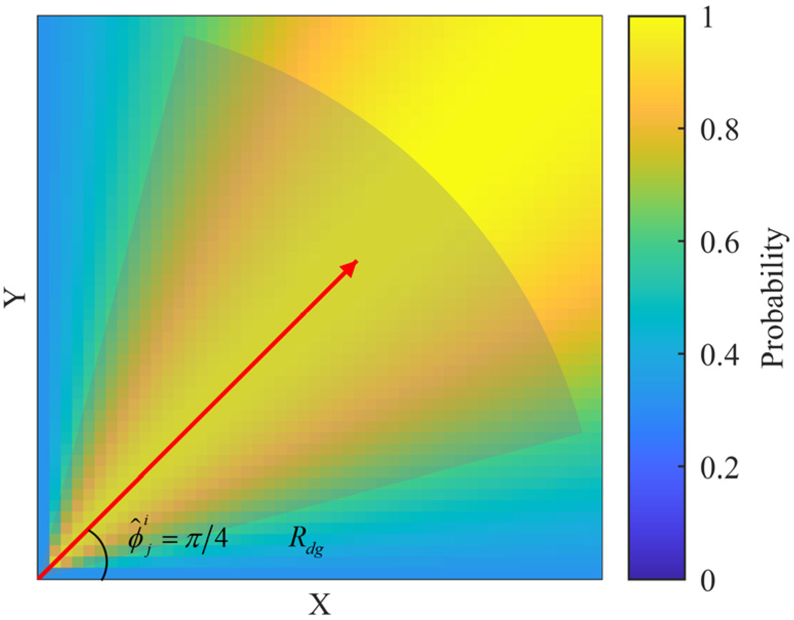
where $F_{ij}$ denotes the repulsive force exerted by $V_j$ on $V_i$. $F_{ij}$ is visualized as the arrow pointing away from $V_j$ toward $V_i$ in Figure 2. $k_f$ denotes the repulsive force coefficient, ${\omega }_f$ denotes the repulsive force factor, $D_{ij}=‖p_{i,k}-p_{j,k}‖$ denotes the value of the distance between the UAVs, and $D_{safe}$ denotes the safe distance between UAVs. $E_{ij}=(p_{j,k}-p_{i,k})/‖(p_{j,k}-p_{i,k})‖$ denotes the unit vector from $V_j$ to $V_i$.

${\phi }_{ij}$ denotes the angle between ${\psi }_i(k)$ and $E_{ij}$, and ${\phi }_{\max }$ denotes the maximum heading angle generated by repulsion. ${\theta }_{uF}$ denotes the angle between the UAV’s position $p_{i,k+1}$ and the repulsive force $F_i(k)$.

As illustrated in Figure 2, the dashed lines with arrows represent the heading direction of each UAV (denoted by ${\psi }_i(k)$ for $V_i$), while ${\phi }_{ij}$ is the angle between the heading direction of $V_i$ and the unit vector $E_{ij}$, and ${\phi }_{\max }$ is the maximum allowable angle for repulsive force activation. ${\theta }_{uF}$ denotes the angle between the position vector of $V_i$ at time $k+1$, $p_{i,k+1}$, and the total repulsive force $F_i(k)$. A dynamic repulsive force is generated only when a neighboring UAV falls within the detection sector defined by $D_{safe}$ and ${\phi }_{\max }$. For instance, $V_j$ generates a repulsive force $F_{ij}$ on $V_i$ because it is within the sector. Conversely, $V_2$ is ignored as it exceeds $D_{safe}$, and $V_1$ is ignored as its relative angle exceeds ${\phi }_{\max }$. The maximum repulsion angle ${\phi }_{\max }$ simulates the limited Field of View (FOV) of directional airborne sensors. From a kinematic perspective, excluding UAVs behind the current UAV prevents unnatural forward acceleration from rear-approaching agents and follows the principle that trailing UAVs are primarily responsible for collision avoidance.

(5)

Obstacle Avoidance Costs: Each prohibited area is modelled as a hemispherical no-fly zone with centre $O_f$ and radius $R_{all}$. The cost of obstacle avoidance is defined as follows:

$$\left\{\begin{array}{l}{d}_f=‖O_f-(p_{i,k}+\widehat{t}(p_{i,k+1}-p_{i,k}))‖\\ C_3(k)=\left\{\begin{array}{ll}0,\hfill & d_f\ge R_{\mathrm{all}}\hfill \\ {\displaystyle \sum _{i=1}^{N_v}\left(R_{\mathrm{all}}-d_f\right)},\hfill & d_f<R_{\mathrm{all}}\hfill \end{array}\right.\end{array}\right.$$

(14)

where $d_f$ is the shortest Euclidean distance from $O_f$ to the path $\overrightarrow{p_{i,k}{p}_{i,k+1}}$, $\widehat{t}={\displaystyle \frac{(O_f-p_{i,k})·(p_{i,k+1}-p_{i,k})}{{‖p_{i,k+1}-p_{i,k}‖}^2}}\in [0,1]$ is the foot of the perpendicular from $O_f$ to the path.

Here $C_1(k)$ penalizes large heading changes, while $C_2(k)$ and $C_3(k)$ act as soft constraints, penalizing small inter-UAV distances and proximity to no-fly zones, respectively. In summary, the overall search performance of the multi-UAV system after the control input $u(k)$ is adopted in the state $x(k)$ is defined as:

$$J^k(x(k),u(k))={\omega }_1{J}_T(k)+{\omega }_2{J}_F(k)-{\omega }_3{C}_1(k)-{\omega }_4{C}_2(k)-{\omega }_5{C}_3(k)$$

(15)

where ${\omega }_l(l=1,\dots ,5)$ are weight coefficients.

The search performance of the multi-UAV system after N-step prediction is modeled as follows:

$$J(X(k),U(k))\triangleq {\displaystyle \sum _{q=0}^{N-1}{J}^{k+q}}(x(k+q|k),u(k+q|k))$$

(16)

$x(k+q|k)$ and $u(k+q|k)$ are the predictions of the system state and control input at time k + q, respectively. The optimization model for solving the optimal task decision of the system at time k can be described as $U^{*}(k)=\arg \underset{U(k)}{\max }J(X(k),U(k))$. Under the DMPC architecture [6], the overall behavior of the system is determined by each subsystem [34,35]. For a decoupled dynamic system, since its state equations are independent of each other, the state equation of the overall system can be expressed as: $f(x(k),u(k))=[f_1(x_1(k),u_1(k)),\dots , f_{N_{\mathrm{v}}}(x_{N_{\mathrm{v}}}(k),u_{N_{\mathrm{v}}}(k))]$, where $f_i(·)$ denotes the state equation of $V_i$. Furthermore, the overall system performance function can be decomposed as:

$$J(X(k),U(k))={\displaystyle \sum _{i=1}^{N_v}{J}_i\{X_i(k),\{X_{j\ne \mathrm{i}}(k)\},U_i(k),\{U_{j\ne \mathrm{i}}(k)\left\}\right\}}(j=1,2,\dots ,N_v)$$

(17)

where $X_i(k)$ and $U_i(k)$ are the N-step predicted state and predicted control input of the $V_i(i=1,2,\dots ,N_v)$, respectively; $\{X_{j\ne \mathrm{i}}(k)\}$ is the set of N-step predicted states of other UAVs; $\{U_{j\ne \mathrm{i}}(k)\}$ is the set of N-step predicted control inputs of other UAVs. Then, the local optimization control model for the subsystem of $V_i$ can be formulated as:

$$\begin{array}{l}{U}_i^{*}(k)=\arg \underset{U_i(k)}{\max }{J}_i\{X_i(k),\{X_{j\ne i}(k)\},U_i(k),\{U_{j\ne i}(k)\}\}\\ s.t.\\ x_i(k+q+1|k)=f_i(x_i(k+q|k),u_i(k+q|k)),\forall q=0,1,\dots ,N-1\\ x_i(k|k)=x_i(k)\\ \underset{q=0,1,\dots ,N-1}{\max }\{|\mathrm{\Delta }{\psi }_i(k+q|k)|-\mathrm{\Delta }{\psi }_{\max }\}\le 0\end{array}$$

(18)

where $U_i^{*}(k)=[u_i^{*}(k),u_i^{*}(k+1),\dots ,u_i^{*}(k+N-1)]$ is the optimal control sequence of $V_i$.

3. Algorithm Design

3.1. Overview of Algorithm Framework

Figure 3 illustrates the CRS-AET framework, consisting of two interactively coupled modules that communicate via a real-time feedback loop. The Target Module (left, blue) uses prior information to initialize the objective spatial distribution and initial physical states of the targets. When a UAV is detected within a target’s reconnaissance range, the target initiates an evasion maneuver; otherwise, it follows a predefined motion rule. To rigorously filter sensor false positives, a target is formally considered detected only when the UAV’s estimated existence probability reaches the threshold $p_m^i(k)\ge {\delta }_p$. Once this threshold is reached, targets are assumed to stop moving to minimize redundant energy consumption. The UAV Module (right, orange) maintains a cognitive belief map, tracking both environmental uncertainty and target existence probability, to enable real-time decision-making and trajectory planning through a cyclic OODA process. The framework introduces three key algorithmic innovations: DG-Prediction (Section 3.2), IMRAA (Section 3.3), and DC-RTO (Section 3.4), which are represented by dark orange blocks in the diagram. The arrow pointing from the target module to the UAV module represents the perception process, that is, the real-time state of the target serves as observation input to update the decision-making information of the UAV; while the feedback arrow pointing from the UAV module to the target module represents dynamic interaction, that is, the optimized UAV path directly induces the target’s evasive behavior or triggers the transition of its detection state by changing the spatial positional relationship. All other components support these core modules and represent standard initialization or physical and cognitive update steps.

Within the UAV module (Figure 3, right), autonomous control is implemented as an embedded OODA (Observe–Orient–Decide–Act) loop, detailed in Figure 4. Each iteration begins by updating UAV and target states from sensors and motion models. DG-Prediction then refines the target probability distribution using current estimates and recent observations. Next, IMRAA dynamically allocates tasks by optimizing auction bids to balance immediate rewards and long-term coverage. Based on task assignments and UAV status, DC-RTO calculates the optimal trajectory that meets the Dubins path conditions for the next planning cycle. While satisfying the kinematic constraints, it maximizes the search objective function as shown in Equation (18). By executing these planned trajectories, the UAVs transition and update their physical states, while simultaneously gathering new observations to mark detected targets and update the probability maps. The three orange modules in Figure 3, DG-Prediction, IMRAA, and DC-RTO, are the core modules in this paper. They interact to adjust and coordinate in real time until all targets are found or the mission times out.

3.2. Directional Gradient-Based Prediction Model

This section presents the core probabilistic reasoning module of CRS-AET, which consists of two interconnected components: the Directional Gradient Probability Update Model and the Graph-Enhanced Probability Diffusion Mechanism. The former generates a directional, discrete probability map, while the latter refines it into a smooth, continuous distribution suitable for cooperative planning.

3.2.1. Directional Gradient Probability Stretching

Traditional probabilistic search methods often rely on isotropic diffusion models to update target existence probabilities across a grid map [19]. These models assume an equal likelihood of the target moving in any direction, which fails to capture the intentional, directional evasion behaviors characteristic of intelligent targets. To address this deficiency, this section proposes the Directional-Gradient Probability Update Model (DG-Prediction). The core innovation of this model lies in introducing a direction-dependent gradient weight coefficient that enables the probability update process to adaptively amplify propagation along the expected evasion direction while attenuating diffusion in other directions. The ultimate objective is to generate an asymmetric, directed probability distribution map that guides the limited UAV resources toward the spatial corridors where the target is most likely to be found.

This model operates on a grid-based distributed probability map. At each decision time $k$ during the inference process, the system performs state evolution based on the posterior probability map $p^i(k-1)$ output by the Bayesian observation fusion module at the previous time $(k-1)$. Since the target is in a non-cooperative state and its true motion direction is unknown, each UAV $V_i$ must conduct an incremental inference of the target’s possible escape direction based on $p^i(k-1)$. Assume that UAV $V_i$ identifies the grid $g_{peak}^i(k-1)$ at time $(k-1)$, which corresponds to the local peak of the probability $p^i(k-1)$, with its center coordinates ${\widehat{p}}_{i,j,k-1}^t=({\widehat{x}}_{t,j}^i(k-1),{\widehat{y}}_{t,j}^i(k-1))$. UAV $V_i$ assumes the target is located at this position and generates an avoidance reaction based on the current position of its own swarm. Thus, according to the avoidance logic in Equations (4)–(6), the expected escape direction angle ${\widehat{\varphi }}_j^i(k)$ estimated by UAV $V_i$ is obtained. For any grid $g_m$ within the target’s influence range, UAV $V_i$ calculates the consistency between its direction from $g_m$ to $g_{peak}^i(k)$ and the expected escape path, which can be expressed as:

$${\theta }_{m,j}^i(k)=\mathrm{atan}2(y_m-{\widehat{y}}_{t,j}^i(k-1),x_m-{\widehat{x}}_{t,j}^i(k-1))$$

(19)

A directional gradient weight coefficient $d^i(m,k)$ is then assigned to each cell, creating a bias towards the expected direction ${\widehat{\varphi }}_j^i$:

$$d^i(m,k)=\left\{\begin{array}{cc}{\omega }_{agg}(k),\hfill & \hfill \mathrm{if}\left|{\theta }_{m,j}(k)-{\widehat{\varphi }}_j^i(k)\right|\le 3{\sigma }_{\theta }\hfill \\ {\omega }_{base}(k)\hfill & \hfill \mathrm{otherwise}\hfill \end{array}\right.$$

(20)

where ${\sigma }_{\theta }$ is the standard deviation of the target’s heading estimate, used to define a $3{\sigma }_{\theta }$ (≈99.7% confidence) expected-direction confidence sector. The weight inside this sector is ${\omega }_{agg}(k)=w_o·v_j^t(k)$, where $w_o=2$ is the directional enhancement gain and $v_j^t(k)$ is the target’s current speed. Outside the sector, the base weight is ${\omega }_{base}(k)=v_j^t(k)$. This coefficient implements two levels of adaptation: (1) directional adaptation, which stretches the probability distribution along ${\widehat{\varphi }}_j^i(k)$; and (2) velocity adaptation, which scales the diffusion strength with the target’s speed, ensuring faster targets induce broader probability spread.

The target existence probability in $g_m$ is updated by integrating the directional weight with the local probability gradient:

$${\tilde{p}}_m^i(k)=p_m^i(k-1)+{\lambda }_d·d^i(m,k)·\left[{\displaystyle \frac{1}{\left|\mathcal{N}(m)\right|}}{\displaystyle \sum _{n\in \mathcal{N}(m)}\left(p_n^i(k-1)-p_m^i(k-1)\right)}\right]$$

(21)

Here, ${\tilde{p}}_m^i(k)$ is the preliminary prediction probability with directional attributes obtained from the calculation, and $p_m^i(k-1)$ is the posterior probability output by the Bayesian observation fusion module at the previous decision step. ${\lambda }_d=0.5$ is the diffusion constant used to control the overall update rate. $\mathcal{N}(m)$ represents the set of 8 neighboring grid cells of $g_m$. The bracket term in the equation is the discrete probability gradient, calculated from the average value difference between $g_m$ and its adjacent grids.

The action of Equation (21) produces a distinct spatial pattern, illustrated conceptually in Figure 5. The grey fan corresponds to a $3{\sigma }_{\theta }$ confidence sector centered on the expected movement direction ${\widehat{\varphi }}_j^i=\pi /4$ (red arrow). The center of this sector is $g_{peak}^i(k)$, and its radius is defined as $R_{dg}=v_{t,j}·P·T_s$, where $P$ is the prediction time domain of DMPC, and $T_s$ is the interval for each domain, i.e., the maximum distance the target can cover within one decision cycle. This fan-shaped emphasis enables the search algorithm to concentrate resources along the most plausible escape corridor.

3.2.2. Graph-Enhanced Probability Diffusion Mechanism

While the directional gradient model described in Section 3.2.1 effectively biases probability updates toward the predicted evasion direction, its output is limited to a discrete, grid-based probability map that may display spatial discontinuities. To address this limitation and produce a spatially continuous, smooth probability distribution that better reflects the continuous nature of target motion, a graph-theoretic diffusion mechanism is introduced. In this approach, the search environment is represented as a graph network, and probability mass propagates along the graph edges through a diffusion process similar to heat conduction. Importantly, this diffusion is directionally modulated to maintain and amplify the directional bias established by the DG-Prediction model.

Graph-Theoretic Representation of the Search Environment

Traditional multi-UAV search algorithms typically discretize the task area into a regular grid, with each grid cell independently storing the probability of target presence. This representation ignores spatial correlations between adjacent grid cells. This paper introduces a graph theory framework to model the discretized search environment as a spatial graph $\mathcal{G}=(\mathcal{V},\mathcal{E})$, where the node set $\mathcal{V}=\left\{g_1,g_2,\dots ,g_M\right\}$ corresponds to the $M=N_x\times N_y$ grid cells and the edge set $\mathcal{E}$ captures spatial adjacency relationships. For the 8-connectivity neighborhood structure:

$$\mathcal{E}=\{(m,n)|g_m \mathrm{and} g_n \mathrm{are} \mathrm{spatially} \mathrm{adjacent}\}$$

(22)

The adjacency matrix $A\in {ℝ}^{M\times M}$ of $\mathcal{G}$ is defined as:

$${[A]}_{mn}=\left\{\begin{array}{ll}1,\hfill & (m,n)\in \mathcal{E}\hfill \\ 0,\hfill & \mathrm{otherwise}\hfill \end{array}\right.$$

(23)

The degree matrix is $D=\mathrm{diag}(d_1,d_2,\dots ,d_M)$, where $d_m={\displaystyle {\sum }_n{[A]}_{mn}}$, and the graph Laplacian is: $L=D-A$.

For an 8-connected spatial topology, each grid node $g_m$ establishes edges with 8 adjacent grid nodes. The edge weight is defined as: $w_{mn}=\exp \left(-{\displaystyle \frac{d_{mn}^2}{2{\sigma }_s^2}}\right)$, where $d_{mn}={‖g_m-g_n‖}^2$ denotes the Euclidean distance between node $g_m$ and node $g_n$, and ${\sigma }_s$ is the spatial scale parameter used to control the attenuation speed of edge weights with distance. This Gaussian-based edge weight definition makes the connection between geographically close nodes stronger, achieving distance-sensitive decay in the continuous probability diffusion process. Each node in the spatial graph is associated with a feature vector for encoding the local environmental state. Due to the adoption of a distributed framework, for the grid cell at time $k$, the local node feature vector $h_m^i(k)\in {ℝ}^{d_h}$ maintained by UAV $V_i$ is defined as:

$$h_m^i(k)={[p_m^i(k),{\chi }_m^i(k),f_m^{geo}]}^T$$

(24)

where $d_h$ is the dimension of the node feature vector, composed of the sum of the dimensions of each component: $p_m^i(k)$ is the target existence probability maintained by UAV $V_i$, ${\chi }_m^i(k)$ is the environmental uncertainty for UAV $V_i$, and $f_m^{geo}$ encodes geometric features such as the distance to regional boundaries and the proximity to no-fly zones. $h_m^i(k)$ encapsulates these three elements in a single data structure, providing a directly usable core structure for posterior task allocation in the local area. The spatial graph G and its node features $\left\{h_m^i(k)\right\}$ together form the core data foundation for subsequent probability diffusion and trajectory planning.

Heat-Diffusion Formulation for Probability Smoothing

In this paper, a multi-UAV collaborative search framework is adopted, where each UAV $V_i$ independently maintains its own directional preliminary prediction probability map ${\tilde{p}}^i(k)={\left[{\tilde{p}}_1^i(k),{\tilde{p}}_2^i(k),\dots ,{\tilde{p}}_M^i(k)\right]}^T\in {ℝ}^M$, as derived in Section 3.2.1. Therefore, the thermal diffusion process is executed independently and in parallel on the local computing nodes of each UAV. By introducing a virtual diffusion time $\tau$, the evolution of the probability distribution on the local map for UAV $V_i$ can be described by the following heat conduction equation:

$${\displaystyle \frac{\partial {\tilde{p}}^i(\tau )}{\partial \tau }}=-\gamma \mathbf{L}{\tilde{p}}^i(\tau )$$

(25)

where $\gamma >0$ is the diffusion coefficient used to control the rate of probability propagation. To improve computational efficiency, a first-order forward Euler discretization with time step $\mathrm{\Delta }t$ is performed, leading to the fundamental discrete diffusion operator:

$${\tilde{\mathit{p}}}^i(\tau +\mathrm{\Delta }t)\approx (I-\gamma \mathrm{\Delta }tL){\tilde{\mathit{p}}}^i(\tau )$$

(26)

where $I$ is the identity matrix. The directional gradient coefficient $d^i(m,k)$ is incorporated into the graph diffusion process by modifying the edge weights of the spatial graph. Due to the distributed framework, each UAV $V_i$ predicts the target escape direction ${\widehat{\varphi }}_j^i(k)$ based on its local perception. For each edge $(m,n)\in \mathcal{E}$ connecting adjacent grid cells, the correction weight calculated by UAV $V_i$ is

$${\tilde{w}}_{mn}^i(k)=w_{mn}\cdot {\kappa }_i({\theta }_{mn},{\widehat{\varphi }}_j^i(k))$$

(27)

where ${\theta }_{mn}$ is the direction angle from the center of cell $g_m$ to cell $g_n$, and ${\kappa }_i(\cdot ,\cdot )$ is a directional kernel function that assigns higher weights to edges aligned with ${\widehat{\varphi }}_j^i(k)$:

$${\kappa }_i({\theta }_{mn},{\widehat{\varphi }}_j^i(k))=\exp \left(-{\displaystyle \frac{{({\theta }_{mn}-{\widehat{\varphi }}_j^i(k))}^2}{2{\sigma }_{\theta }^2}}\right)$$

(28)

Based on the corrected edge weights, the direction modulation graph Laplacian matrix specific to the UAV $V_i$ is:

$${\tilde{L}}^i(k)={\tilde{D}}^i(k)-{\tilde{A}}^i(k)$$

(29)

where the modified adjacency matrix ${[{\tilde{A}}^i(k)]}_{mn}={\tilde{w}}_{mn}^i(k)$ and ${\tilde{D}}^i(k)$ is the corresponding degree matrix. Replacing the standard Laplacian $L$ in Equation (26) with the directionally modulated version ${\tilde{L}}^i(k)$. The final graph-enhanced diffusion is updated as follows:

$${\mathit{p}}_s^i(k)=(I-\gamma \mathrm{\Delta }t{\tilde{L}}^i(k)){\tilde{\mathit{p}}}^i(k)$$

(30)

The output ${\mathit{p}}_s^i(k)={\left[p_{s,1}^i(k),p_{s,2}^i(k),\dots ,p_{s,M}^i(k)\right]}^T\in {ℝ}^M$ is a spatially smooth probability distribution field that maintains directional emphasis on the predicted evasion corridor, exhibits natural spatial continuity by removing artificial grid-based discontinuities, and respects the graph topology of the environment. This refined distribution is subsequently used for task allocation and trajectory optimization.

Thus, this paper constructs a direction-aware probability prediction model that completes the transition of the probability distribution from the posterior state at $(k-1)$ to the prior state ${\mathit{p}}_s^i(k)$ at time $k$. This optimized prior predictive probability ${\mathit{p}}_s^i(k)$ is directly fed as input into Equation (15) from Section 2.4.2. By fusing it with the actual sensor detection results at time $k$, the system can compute the final posterior probability map ${\mathit{p}}^i(k)$ and initiate the next round of decision-making. This enhanced probability diffusion mechanism ensures the sustained state tracking capability of the multi-UAV system in a dynamically evolving environment.

3.3. Improved Multi-Round Auction Algorithm

Effective cooperative search relies on dynamic and efficient task allocation to prevent multiple UAVs from covering the same area or competing for the same target, which would otherwise lead to resource waste and low search efficiency. Traditional allocation methods, such as static partitioning [36] or basic auction mechanisms [8], often neglect the dynamic evolution of target probability maps, which tends to cause UAV swarms to cluster in local hotspots and hinders the achievement of wide-area and balanced coverage. To address this issue, this subsection proposes the Improved Multi-Round Auction Algorithm (IMRAA). By integrating a distance-based incentive mechanism, a load balancing mechanism, and a graph-based utility propagation mechanism, this algorithm extends traditional auction methods. It is designed to achieve three core objectives: (1) rapid response: enabling UAVs to prioritize the processing of adjacent high-probability targets; (2) wide-area coverage: incentivizing some UAVs to explore long-distance regions to prevent premature swarm convergence; (3) load balancing: avoiding concurrent competition among multiple UAVs for the same task through implicit coordination.

3.3.1. Utility Function Design

IMRAA quantifies the expected utility of a UAV performing the search task for a target using a comprehensive utility function. This utility function incorporates three key factors: distance cost, exploration incentive, and load balancing. The utility of task allocation for target $T_j$ by UAV $V_i$ is defined as follows:

$$u_{ij}(k)=\alpha ·\left(1-{\displaystyle \frac{{\widehat{d}}_{ij}(k)}{d_{\max }}}\right)+\beta ·{\left({\displaystyle \frac{{\widehat{d}}_{ij}(k)}{d_{\max }}}\right)}^2+\rho ·\left(1-{\displaystyle \frac{n_j(k)}{n_{\max }}}\right)$$

(31)

where ${\widehat{d}}_{ij}(k)$ denotes the distance between $V_i$ and the predicted position of the moving target $T_j$ estimated by $V_i$, ${\widehat{d}}_{ij}=‖p_{i,k}-{\widehat{p}}_{i,j,k}^t‖$. $d_{\max }$ is the maximum distance between $V_i$ and $T_j$. In order to avoid drastic turning of the UAV during the assignment process, set the angular deviation $\mathrm{\Delta }{\psi }_{i\to j}$ between $V_i$ and $T_j$, $\mathrm{\Delta }{\psi }_{i\to j}\le \mathrm{\Delta }{\psi }_{\max }$ when the target assignment can be performed. $\left[1-({\widehat{d}}_{ij}(k)/d_{\max })\right]$ represents the distance factor ensuring the UAV prioritizes selecting closer targets. This term ensures that UAVs prioritize closer targets, thereby optimizing resource allocation and reducing energy consumption. Conversely, ${\left({\widehat{d}}_{ij}(k)/d_{\max }\right)}^2$ denotes the distance incentive term, which enhances the attractiveness of distant targets as the distance grows. This mechanism prevents the UAV swarm from clustering around nearby targets and promotes broader area coverage. Additionally, $\left[1-(n_j(k)/n_{\max })\right]$ is a balancing factor that encourages UAVs to select less crowded targets, where $n_j$ denotes the current number of UAVs assigned to a target, and $n_{\max }$ is the maximum allowed. $\alpha$, $\beta$, and $\rho$ are the weighting coefficients. This paper sets $n_{\max }=2$, $\alpha =0.4$, $\beta =0.3$, $\rho =0.3$.

3.3.2. Graph-Based Utility Propagation

To enhance coordination in task allocation and prevent multiple UAVs from competing for the same hotspot area, we introduce a graph-based utility propagation mechanism within IMRAA. This mechanism allows each UAV to consider the preferences of neighboring UAVs when making bidding decisions, thereby reducing redundant assignments and improving overall search efficiency.

Let $G_{uav}(k)=(V,E_{uav}(k))$ represent the communication network among UAVs at time k, and $E_{uav}(k)=\{e_{ij}(k)=(V_i,V_j):V_i,V_j\in V;‖p_{i,k}-p_{j,k}‖\le R_{comm}\}$. $R_{comm}$ denotes the communication radius. The adjacency matrix $A_{uav}(k)$ is defined as:

$$A_{uav}(k)={[a_{ij}(k)]}_{N_v\times N_v},a_{ij}(k)=\left\{\begin{array}{ll}1,\hfill & \mathrm{if} e_{ij}(k)\in E_{uav}(k)\mathrm{and} i\ne j\hfill \\ 0,\hfill & \mathrm{otherwise}.\hfill \end{array}\right.$$

(32)

For the UAV interaction graph, the degree matrix $D_{uav}(k)$ is a diagonal matrix with elements:

$${[D_{uav}(k)]}_{ii}={\displaystyle \sum _{j=1}^{N_v}{\left[A_{uav}(k)\right]}_{ij}}$$

(33)

The row-normalized propagation matrix is then computed as:

$$P_{uav}(k)=D_{uav}^{-1}(k)A_{uav}(k)$$

(34)

This normalization ensures that each UAV distributes its influence equally among its neighbors. For isolated UAVs with zero degree, the corresponding row of $P_{uav}(k)$ is set to zero. Assuming there is no correlation between the targets, $P_{target}(k)=I$. The utility matrix after propagation on the UAV communication graph $\tilde{U}(k)$ is calculated by integrating the original utility with information from the two types of propagation graphs:

$$\tilde{U}(k)=U(k)+\mu P_{uav}(k)U(k)+\nu U(k)P_{target}(k)$$

(35)

where $U(k)\in {ℝ}^{N_v\times N_t}$ is the original utility matrix with ${[U(k)]}_{ij}=u_{ij}(k)$. The first term, $P_{uav}(k)U(k)$, indicates that each UAV evaluates its utility relative to its neighboring UAVs. If a neighbor exhibits high utility toward a target, the UAV itself tends to avoid it, thereby achieving implicit coordination among UAVs. The second term, $U(k)P_{target}(k)$, indicates that the utility for a target propagates to its neighboring targets, i.e., This enables UAVs to focus on target clusters rather than isolated points, promoting comprehensive coverage of target-rich regions. $\mu \ge 0$, $\nu \ge 0$ are tuning parameters controlling the strength of UAV-to-UAV and target-to-target propagation, respectively. Ultimately, the auction algorithm bases bids on the propagated utility ${[\tilde{U}(k)]}_{ij}={\tilde{u}}_{ij}(k)$, significantly reducing task conflicts.

In each round of the auction, unassigned UAVs will bid based on the propagated utility ${\tilde{u}}_{ij}(k)$ and the local public price $p_{ij}$. The local public price $p_{ij}$ of the $V_i$ are equal for each UAV. The bid price $b_{ij}$ offered by $V_i$ for $T_j$ is:

$$b_{ij}(k)={\tilde{u}}_{ij}(k)-p_{ij}$$

(36)

For $V_i$, select the target that delivers the highest benefit, denoted by $T_{j^{*}}$ as follows:

$$T_{j^{*}}=\arg \underset{T_j\in T}{\max }{b}_{ij}(k)$$

(37)

If a target is searched in a given round, the target drops out of the running for reassignment. The algorithm repeats until all targets have been assigned.

Algorithm 1 provides a detailed description of the dynamic task allocation process. The multi-round nature of the auction allows for reallocation as the search environment evolves, while the graph-based propagation ensures coordinated decision-making across the UAV team. Algorithm 1 outputs the specific target assignment, which directly serves as the reference destination in the DMPC objective function.

Algorithm 1: Improved Multi-Round Auction Algorithm, IMRAA

$\mathbf{Input}\mathbf{:} \mathrm{UAVs}’ \mathrm{position}, \mathrm{targets}’ \mathrm{position}, n_{\max }$ Output: task allocation results

1: $\mathbf{while} \mathrm{any} \mathrm{UAV} \mathrm{unassigned} \mathrm{and} iter< 100$do 2: $iter\leftarrow iter + 1$ 3: $\mathrm{Initialize} b_{ij}\leftarrow 0$ 4: $\mathbf{Calculate} \mathbf{original} \mathbf{utility} \mathbf{matrix} U(k)$ 5: $\mathbf{for} i\leftarrow 0$. to Nv do 6: $\mathbf{for} j\leftarrow 0$$\mathbf{to} N_t$ do 7: $\mathrm{limit} \mathrm{\Delta }{\psi }_{i\to j}\le \mathrm{\Delta }{\psi }_{\max }$; 8: $\mathrm{Calculate} \mathrm{utility} u_{ij}$ by Equation (31); 9:     end for 10:  end for 11:  Graph-Based Utility Propagation using Equations (32)–(35). 12: $\mathbf{Each} \mathbf{UAV} \mathbf{submits} \mathbf{bids} \mathbf{for} \mathbf{targets} \mathbf{based} \mathbf{on} \mathbf{the} \mathbf{propagated} \mathbf{utilities} \tilde{U}(k)$. 13: $\mathrm{Calculate} b_{ij}$ using Equation (36); 14:  Task allocation: 15:  for each unassigned $V_i$. do 16: $\mathrm{Find} \mathrm{target} T_{j^{*}}$ with max bid for $V_i$ by Equation (37); 17: $\mathrm{Update} \mathrm{and} \mathrm{assign} T_{j^{*}}$ to $V_i$; 18:  end for 19: end while

3.4. Trajectory Planning

The existing trajectory optimization methods for fixed-wing UAVs decouple path feasibility and kinematic constraints [37], resulting in suboptimal or infeasible solutions in dynamic environments. In contrast, we propose a DC-RTO method that is tightly integrated into the DMPC framework. Our innovation lies in the encoding of Dubins curvature constraints into the search space, and in the tailored preparation of decision variables, i.e., sequences of heading angle adjustments for each UAV over the prediction horizon. To efficiently solve this nonlinear and non-convex problem, we adapt the particle swarm optimization (PSO) approach [38]. However, unlike conventional PSO, we redesign the population initialization and constraint handling to exploit the structure of cooperative multi-UAV search fully. Specifically, rather than relying on the fitness function to softly penalize impossible sharp turns, which forces the PSO to waste computational resources exploring “unflyable” trajectories. We embed Dubins constraints strictly, guaranteeing that every evaluated particle is physically flyable. This enables our algorithm to achieve both real-time performance and guaranteed kinematic feasibility.

Each particle in the swarm represents a candidate solution encoding specific heading adjustments for all UAVs over all steps in the horizon [39], the fitness of each particle is evaluated by directly computing the comprehensive DMPC objective function. By minimizing this unified objective function, the PSO algorithm bridges the gap between high-level task assignment and low-level safe, feasible trajectory execution. For a given particle, the algorithm simulates the resulting multi-UAV trajectories: starting from the UAVs’ current states, it applies the candidate heading changes up to P steps ahead. P is the prediction time domain of DMPC. For $V_i$, at the k-th time domain $k=(1.2,\dots ,P)$, the heading angle is: ${\psi }_i(k)={\psi }_i(k-1)+\mathrm{\Delta }{\psi }_i(k-1)$. During this simulation, limit any proposed turn $\mathrm{\Delta }{\psi }_i(k)<\mathrm{\Delta }{\psi }_{\max }$ to maintain feasibility.

In this paper, the UAV is set to fly at a constant speed $v_u$. According to the prediction window interval time $T_s$, the UAV is sampled on the path to obtain the distance $d_{i,k}$ that the UAV moves in $T_s$, $d_{i,k}=v_u·T_s$. The motion equation for each UAV is expressed as follows:

$$p_{i,k}^{goal}=p_{i,k}+d_{i,k}·\left[\begin{array}{c}\cos {\psi }_i(k)\\ \sin {\psi }_i(k)\end{array}\right]$$

(38)

where $p_{i,k}=(x_{u,i}(k),y_{u,i}(k))$ is the current position of $V_i$ and $p_{i,k}^{goal}=(x_{u,i}^{goal}(k),y_{u,i}^{goal}(k))$ denotes the end position reached by the UAV after $T_s$.

In order to generate smooth and kinematically constrained trajectories, Dubins path planning is used. The Dubins path is the shortest path whose path curvature does not exceed the maximum curvature ${\kappa }_{\max }=1/R_{\max }$ for a given starting state $q_{i,k}^{start}=\left[p_{i,k},{\psi }_i(k)\right]$ and ending state $q_{i,k}^{goal}=\left[p_{i,k}^{goal},{\psi }_i(k+1)\right]$. Dubins path consists of three parts: left turn (L), right turn (R), and straight ahead (S), with a total of six combinations of RSR, LSL, RSL, LSR, RLR, and LRL [40]. Calculate the path lengths for all Dubins path types and select the shortest path as optimal $L_{i,k}$. If $d_{i,k}>L_{i,k}$, the UAV can reach the target’s required attitude within the current step $T_s$, the trajectory is adjusted accordingly; Otherwise, an intermediate Dubins-compliant heading is computed using Equation (38) by interpolating along the Dubins path proportionally to $d_{i,k}/L_{i,k}$:

$$p_{i,k+1}=p_{i,k}+{\displaystyle \frac{d_{i,k}}{L_{i,k}}}(p_{i,k+1}^{goal}-p_{i,k})$$

(39)

Throughout the simulated horizon, the fitness function Equation (18) evaluates the quality of the particle’s solution. A higher fitness indicates a more optimal trajectory. The PSO iteratively improves these candidate solutions. At each iteration, the algorithm updates particle velocities and positions using the PSO update rules. Through many such iterations, the swarm converges toward an optimal or near-optimal set of heading commands. The system then executes only the first command of the current optimal control sequence and performs rolling optimization at the next time step using the latest environmental information. When a convergence or stopping criterion is met, the global best particle encodes the optimal Dubins-constrained trajectories. The heading adjustments from this best particle are decoded as the final control output $u_i^{*}(k)$ for each UAV.

Algorithm 2 details the DC-RTO-based path planning procedure, ensuring that all candidate trajectories are physically feasible for UAVs.

Algorithm 2: Dubins-Constrained Trajectory Optimization, DC-RTO

$\mathbf{Input}\mathbf{:} \mathrm{Initial} \mathrm{State} \mathrm{of} \mathrm{Multi}-\mathrm{UAVs}. \mathrm{PSO} \mathrm{parameters}: \mathrm{Maximum} \mathrm{iterations} N_{pso}$$, \mathrm{population} \mathrm{size} M_{pop}$ $\mathbf{Output}\mathbf{:} \mathrm{Optimal} \mathrm{control} \mathrm{sequence} u_i^{*}(k)$

1: $\mathbf{for} iter=1$$\mathrm{to} N_{pso}$ do 2: $\mathbf{for} \mathrm{each} \mathrm{particle} pop=1$$\mathbf{to} M_{pop}$ do 3: $\mathbf{for} \mathrm{each} \mathrm{UAV} i=1$$\mathbf{to} N_v$ do 4: $\mathbf{for} k=1$ to $P$ do 5: $\mathrm{Heading} \mathrm{feasibility}: \mathrm{Limit} \mathrm{\Delta }{\psi }_i(k)<\mathrm{\Delta }{\psi }_{\max }$; 6:        UAV state propagation with Dubins compliance: 7: $\mathrm{Calculate} d_{i,k}$$, \mathrm{Calculate} p_{i,k+1}^{goal}$$\mathrm{by} \mathrm{Equation} \left(38\right), \mathrm{generate} \mathrm{Dubins} \mathrm{path} L_{i,k}$; 8: $\mathrm{Update} p_{i,k+1}$ using Equation (39); 9:      end for 10:   end for 11: $\mathbf{Trajectory} \mathbf{evaluation}\mathbf{:} \mathrm{Get} U_i^{*}(k)$ using fitness function Equation (18); 12: $\mathrm{Update} \mathrm{individual} \mathrm{best} p_{best}$$\mathrm{and} \mathrm{global} \mathrm{best} g_{best}$ of PSO; 13:  end for 14: Update all particles’ velocities and positions using PSO rule. 15: end for 16: $\mathrm{Obtain} \mathrm{optimal} \mathrm{control} \mathrm{signals} u_i^{*}(k)$$\mathrm{for} \mathrm{each} V_i$.

3.5. Overall Process of the Proposed Algorithm

Algorithm 3 outlines the complete CRS-AET workflow for multi-UAV cooperative search after initializing the UAV and target parameters, including position, velocity, heading, sensing range, and map resolution. The algorithm enters a main loop that terminates when all targets are detected or the maximum mission time has elapsed.

At the start of each iteration, the DG-prediction model updates the target probability map and generates predicted positions and headings for all undetected targets. These predictions are then fed to Algorithm 1 to perform dynamic task allocation. Next, Algorithm 2 computes the optimal control sequence for each UAV, producing Dubins-feasible trajectories that update their paths in real-time. Throughout the loop, CRS-AET logs detection events and coverage statistics evaluates mission completion and stores the resulting data for post-analysis.

Algorithm 3: Cooperative Rapid Search Algorithm for Evasive Targets, CRS-AET

$\mathbf{Input}\mathbf{:} p_{i,k}=(x_{u,i}(k),y_{u,i}(k))$$, p_{j,k}^t=(x_{t,j}(k),y_{t,j}(k))$$, N_v$$, N_t$, $N$, $P$, $T_s$. Output: Target search results

1: $\mathbf{Initialization}\mathbf{:} end\_flag=0$$, k\leftarrow 0$ 2: $\mathbf{while} end\_flag=0$ do 3: $\mathrm{Update} k\leftarrow k+1$ 4:   Get current positions of UAVs and targets. 5:   Directional-Gradient Motion Prediction Model: 6: $\mathbf{for} \mathrm{each} \mathrm{target} Tj$ do 7:     if detected: Keep target at current position. 8:     else: Predict target positions using Equation (4). 9:   end for 10:  Improved Multi-Round Auction Algorithm: 11:  Solve multi-round auction for UAV-target assignment using Algorithm 1. 12:  Optimize UAV control signals: 13: $\mathrm{Adopt} \mathrm{Algorithm} 2 \mathrm{to} \mathrm{calculate} \mathrm{UAV} \mathrm{control} \mathrm{signals} u_i^{*}(k)$. 14:  Update UAV positions and states in each control time domain: 15: $\mathbf{for} j\leftarrow 1$ to $N$ 16: $\mathbf{for} \mathrm{each} \mathrm{UAV} i\leftarrow 1$$\mathbf{to} N_v$ 17: $\mathrm{Update} \mathrm{UAV} \mathrm{positions} \left(x_{u,i}(k),y_{u,i}(k)\right)$$\mathrm{and} \mathrm{headings} {\psi }_i(k)$$\mathrm{by} u_i^{*}(k)$ 18:     end for 19:   Compute and store new target positions using Equation (4) 20:   Update environmental information map model using Equations (7)–(11). 21:   Check termination conditions: 22:     if all targets detected 23: $\mathrm{Set} end\_flag\leftarrow 1$ 24:     end if 25:   end for 26: end while

4. Simulations and Results

This section elaborates on the comprehensive simulation experiments conducted for the systematic evaluation of the proposed algorithm. The evaluation first verifies the basic performance of the DG Prediction Module, then examines the integrated performance of task allocation and trajectory planning in complex multi-objective scenarios, and subsequently identifies the specific contribution of graph-theoretic modeling through ablation experiments. This methodology provides empirical support for the effectiveness of the CRS-AET Framework and its core components from multiple dimensions. Finally, hardware-in-the-loop simulation is carried out to further verify the robustness and feasibility of the CRS-AET Framework in practical applications.

The proposed target search strategy is verified through two types of simulations, starting with numerical simulations which are divided into two parts: Part 1 tests the core algorithm components such as target motion prediction and task allocation strategies. Each experiment is configured with 30 independent simulation runs to ensure the statistical significance and reproducibility of the results. The simulations are implemented on MATLAB R2024a, based on an Intel Core i5-9500 CPU (3.00 GHz) and a 64-bit Windows 10 operating system. Part 2 evaluates the graph-theoretic modeling and deep learning components using public datasets; these components are developed based on Python 3.9 and PyTorch 2.0, running on a 64-bit Ubuntu 20.04 operating system. The hardware-in-the-loop (HIL) simulation platform is Rflysim3D Fullv4.00, which is deployed on a 64-bit Windows 10 operating system.

4.1. Simulation Setup

4.1.1. Simulation Parameter Settings

The mission area is set to be 6000 m × 6000 m, discretized into a 100 × 100 grid. The number of grids $M=10000$. Suppose UAVs’ initial positions are (100, 100), (1000, 100), (2000, 100), (3000, 100), (4000, 100), (5000, 100), (6000, 100), $N_v=7$. To enhance the readability and present the experimental setup systematically, all detailed parameters, including environment settings, UAV kinematics, sensor capabilities, DMPC settings, and optimization weights, are summarized in

Table 1. Summary of Main Simulation Parameters.

Category	Parameter Description	Symbol	Value
Initial Setup	Number of grids	$M$	10,000
	Number of UAVs	$N_v$	7
	Speed of the UAV	$v_u$	25 m/s
	Initial heading angle	$\psi \left(0\right)$	$\pi /2$ rad
UAV Kinematics & Sensors	Minimum turning radius	$R_{\min }$	80 m
	Maximum turning angle	$\mathrm{∆}{\psi }_{\max }$	$\pi /4$ rad
	Reconnaissance radius	$R_s$	800 m
	Target perception range	$R_t$	900 m
	Detection/False alarm probability	$p_d$$/p_f$	0.8/0.2
	Communication radius	$R_{comm}$	2000 m
Problem Formulation	Std. dev. of target probability	${\delta }_0$	600 m
	Safe distance between UAVs	$D_{safe}$	100 m
	Repulsion coefficient	$k_f$	1
	Repulsion factor	${\omega }_f$	0.1
	Max heading angle by repulsion	${\phi }_{\max }$	$3\pi /2$ rad
	Trajectory planning weights	${\omega }_1,{\omega }_2,{\omega }_3,{\omega }_4,{\omega }_5$	$100, 80, 20, 100, \mathrm{l}e+5$
Task Allocation	Local public price	$p_{ij}$	0.8
	The maximum distance between UAVs and targets.	$d_{\max }$	6000 m
DMPC	Control/Prediction time domain	$N/P$	3/3
	Interval for each domain	$T_s$	5 s
PSO	Max iterations/Population size	$N_{pso}$$/M_{pop}$	50/20
Graph-based Components	Spatial graph connectivity	—	8-connectivity
	Spatial scale parameter	${\sigma }_s$	100 m
	Diffusion rate parameter	$\gamma =0.1$	0.1
	Directional kernel parameter	${\sigma }_{\theta }$	$\pi /6$
	Utility propagation coefficients	$\mu$, $\nu$	0.2, 0.1

.

In the experimental initialization, all fixed-wing UAVs are configured to enter the mission area simultaneously from one side of the map. This specific deployment pattern was deliberately designed to reflect the logistical constraints of real-world UAV flight projects. Unlike multirotor drones, fixed-wing UAVs require dedicated runways for takeoff and recovery. Consequently, they are typically deployed from a single ground control base and enter the operational airspace through a unified corridor.

For the trajectory planning module, the control time domain of DMPC is $N=3$, the prediction time domain of DMPC is $P=3$, and the interval for each domain is $T_s=5 \mathrm{s}$, each DMPC optimization yields a feasible trajectory spanning a future horizon of 15 s. Furthermore, for the graph-based components introduced in this paper, the neural network architecture is implemented using the PyTorch Geometric library 2.8.0, leveraging message passing layers for efficient spatial information aggregation. The specific topological structures (e.g., 8-connectivity) and propagation coefficients are also detailed in Table 1.

4.1.2. Dataset Description

In addition to the simulation-based evaluation, the Stanford Drone Dataset [41] is employed to validate the proposed algorithm with realistic trajectory data. This dataset contains aerial imagery captured by drones over university campus environments, providing trajectory annotations for various moving agents including pedestrians, cyclists, and vehicles. The dataset encompasses diverse movement patterns and evasive behaviors that align with the intelligent target avoidance scenarios considered in this paper. To adapt the dataset for multi-UAV cooperative search validation, trajectory segments exhibiting directional changes and avoidance-like behaviors are extracted and mapped onto the grid-based search environment. The original pixel coordinates are transformed into the 6000 m × 6000 m mission area through appropriate scaling factors. A simulation-based data augmentation procedure is employed to generate synthetic target trajectories by perturbing the original paths with directional noise following the Gaussian distribution described in Section 3.2.

4.2. Evaluation of Core Algorithm Components

4.2.1. Evaluating the Effectiveness of Target Motion Prediction

A scenario was designed to evaluate the impact of target motion prediction, featuring evasive targets with randomly varying trajectories. To systematically assess the contribution of each algorithmic component, an ablation study was conducted, comparing four methods. All methods generate flight paths using the proposed DC-RTO trajectory planner for a fair comparison. The compared methods are as follows:

• Gaussian-Prediction Baseline [19] (GP-Baseline): This simple baseline uses a basic Gaussian error model for target motion prediction and does not employ our proposed IMRAA for task allocation.
• DG-Prediction: This variant uses our proposed DG-Prediction for target motion prediction but excludes task allocation.
• IMRAA-Gaussian: This method uses the IMRAA task allocator but relies on the Gaussian prediction model from [19].
• CRS-AET: Our complete algorithm, integrating the proposed DG-Prediction for target motion modeling and IMRAA for cooperative task allocation.

This comparison aims to isolate and quantify the individual and combined benefits of our novel prediction and allocation modules for searching evasive targets. The computational load was measured by recording the average time per step and the total number of steps required for the UAVs to complete the search task. The initial information of the targets is shown in

Table 2. Initial state of targets in the first simulation.

Label	Initial Position	Initial Velocity (m/s)	Initial Heading (Rad)
$T_1$	(3000, 1500)	8	$\pi /2$
$T_2$	(500, 2300)	8	0
$T_3$	(1200, 5000)	8	0
$T_4$	(5000, 2500)	8	$\pi /2$

.

Figure 6 shows the final paths obtained by different algorithms, with UAV initial positions represented by blue solid dots. A distinct colored curve depicts each UAV’s trajectory, while red solid dots mark the initial positions of targets, and red solid lines show their motion paths. When targets moved slowly or were close to UAVs, the benefit of motion prediction was limited—all algorithms successfully located the initial targets within 25 steps. However, as targets began moving evasively and unpredictably, the performance gap between prediction methods became apparent. When searching for $T_4$, Gaussian-Prediction Baseline often failed to adapt to rapid trajectory changes, leading to UAV hesitation and increased repositioning. In contrast, DG-Prediction allowed UAVs to anticipate directional shifts more accurately, reducing response delays and improving tracking continuity. Further comparisons in Figure 6 show that DG-Prediction improved target interception paths, adding task allocation via IMRAA resulted in even more efficient UAV distribution and better cooperative behavior. For instance, Figure 6b vs. Figure 6d reveals that without allocation, UAVs still tended to cluster, whereas with IMRAA, they dispersed strategically to maximize area coverage and minimize overlap. Overall, motion prediction enhanced foresight in dynamic target tracking, and task allocation ensured optimal role division among UAVs.

Figure 7a,b plot the average number of targets detected and the average coverage curves of different algorithms during the search process, respectively.

Table 3. Comparison of performance metrics for motion prediction algorithms.

Algorithm	Steps	Coverage (%)	Avg. Time Per Steps (s)	ΔSteps vs. GP-Baseline	ΔCoverage vs. GP-Baseline
GP-Baseline	77	83.97	9.37	—	—
DG-Prediction	75	69.61	9.17	−2.60%	−17.09%
IMRAA-Gaussian	51	61.89	9.40	−33.77%	−26.30%
CRS-AET	48	57.19	9.09	−37.66%	−31.89%

summarizes the final results, specifically including the iterative steps required to detect all targets, the coverage rate at completion, and each method’s relative improvement or reduction compared to Baseline.

As shown in Table 2, GP-Baseline completed the task in 77 steps with a 83.97% coverage rate. Our DG-Prediction model improved search efficiency by 2.60% but reduced coverage by 17.09%, indicating a more targeted yet less exhaustive search. Through task allocation via IMRAA, the full CRS-AET method achieved the best performance: it required only 48 steps, which is 37.66% faster than the baseline, while maintaining a 57.19% coverage rate, 31.89% lower than GP-Baseline. This demonstrates that while dynamic prediction improves responsiveness, intelligent allocation is crucial for search efficiency. The average computational time per iteration remained similar across algorithms, indicating that CRS-AET’s gains do not come at an additional computational cost.

These results validate that DG-Prediction outperforms traditional Gaussian modeling by adapting to real-time movement trends. More importantly, when combined with IMRAA task allocation, the system achieves significant gains in both search speed and coordination. The proposed method CRS-AET thus provides a robust solution for dynamic and evasive search environments.

4.2.2. Evaluating Task Allocation Strategies

To ensure a fair and isolated evaluation of the task allocation module, all compared methods share an identical algorithmic foundation except for their assignment logic. Specifically, each method utilizes the same DG-Prediction module for target motion forecasting and the same DC-RTO module for trajectory planning. This common configuration guarantees that any performance difference stems solely from the task allocation strategy. Three representative strategies are compared:

• No-Allocation [16]: A baseline method without explicit coordination, where each UAV makes independent search decisions based on a shared information map.
• DHBA [42]: Decentralized Hungarian-based algorithm, a distributed, communication-limited strategy where each UAV builds a local cost matrix and exchanges information only with its immediate neighbors.
• IMRAA: Our integrated strategy featuring a distance-based incentive, load balancing, and graph-based utility propagation for implicit coordination.

The evaluation employs three distinct scenarios to rigorously test the adaptability and efficiency of these allocation mechanisms under complex search conditions.

Scenario 1: Uneven Target Distribution with No-Fly Zones

In the simulation setup, the targets are distributed across two regions: one region contains densely clustered targets near the UAV’s starting point, while the other region contains sparsely distributed targets located farther away. Two circular no-fly zones are present in the environment, each defined by centre $O_f$ and radius $R_w=300 \mathrm{m}$. Specifically, $O_{f1}=(1600,4000)$, $O_{f2}=(4700,2800)$. The initial information of the targets in the three comparison algorithms is summarized in

Table 4. Initial target information for Scenario 1.

Label	Initial Position	Initial Velocity (m/s)	Initial Heading (Rad)	Region
$T_1$	(3000, 1500)	8	0	Dense
$T_2$	(500, 2300)	8	0	Dense
$T_3$	(2700, 4200)	8	$\pi /2$	Sparse
$T_4$	(1500, 4800)	8	0	Sparse
$T_5$	(5500, 5000)	0	0	Sparse

.

Figure 8 presents the final UAV search trajectories for the three algorithms. Each no-fly zone has a safety boundary represented by a dashed line with a radius of $R_m=150 \mathrm{m}$, $R_{all}=R_w+R_m=450 \mathrm{m}$. Figure 9a,b display the average number of targets detected and the average coverage curves for each algorithm during the search process.

Table 5. Algorithm indicators comparison in Scenario 1.

Algorithm	Steps	Coverage (%)	Avg. Time Per Steps (s)	ΔSteps vs. No-Allocation	ΔCoverage vs. No-Allocation
No-Allocation	80	76.05	11.26	—	—
DHBA	67	52.42	11.01	−16.25%	−31.33%
IMRAA	47	60.28	11.03	−41.25%	−20.74%

summarizes the search performance metrics.

The comparative results in Table 5 and the trajectory visualizations in Figure 8 enable a detailed analysis of the performance of the three task allocation strategies as follows:

First, the No-Allocation method required the longest search duration (80 steps) but achieved the highest area coverage (76.05%). This extensive coverage results from the absence of explicit coordination, which causes UAVs to operate independently. As illustrated in Figure 8a, UAVs initially converge toward the target-dense region but subsequently display wandering and overlapping search patterns. This behavior leads to frequent revisits to areas with locally high probability, resulting in significant redundancy and inefficiency despite broad coverage. In contrast, the DHBA method improved search efficiency, completing the mission in 67 steps, but achieved the lowest coverage (52.42%). Its distributed, neighbor-consensus mechanism forms stable, local subteams, as shown in Figure 8b, where UAVs split into two distinct clusters. Each cluster optimizes assignments within its local communication neighborhood but lacks global coordination. This limitation leads to prolonged concentration in specific sectors, poor dispersion across the search area, and, consequently, fragmented and incomplete coverage. Finally, the IMRAA method demonstrated the best overall performance, locating all targets in 47 steps, which represents reductions of 41.25% and 29.85% compared to No-Allocation and DHBA, respectively, while maintaining balanced coverage of 60.28%. The integrated graph-based utility propagation enables implicit global coordination. As shown in Figure 8c, UAVs are effectively dispersed from the outset, avoiding initial clustering. The distance-based incentive and load-balancing mechanisms dynamically guide UAVs toward less-visited and distant high-value areas, minimizing redundant paths and ensuring efficient, non-overlapping exploration of the entire region.

The average computation time per step remains similar for all three methods, approximately 11 s, indicating that the enhanced coordination provided by IMRAA does not incur additional online computational cost.

Scenario 2: UAV Failure During Search

To assess the robustness of different task allocation strategies in the presence of unexpected UAV failures, a failure event is introduced during the search process. One UAV is randomly removed from operation, simulating real-world failures such as hardware malfunctions or power depletion. It is worth noting that it follows the conditions described in Scenario 1, maintaining the same target distribution and motion patterns outlined in Table 4.

In Scenario 2, UAV 4 exits at Step = 30, represented by the blue dot in Figure 10. This reduces the available fleet and challenges the algorithm’s ability to dynamically reallocate tasks. Figure 11a,b present the average number of targets detected and the average coverage curves of different algorithms during the search process. In Figure 11b, the red solid points represent the exit times of UAV 4. The black dashed line connects the red solid points to the coverage curve, indicating the proportion of the search area covered by the algorithm at the time of the UAV’s exit.

Table 6. Search performance comparison in Scenario 2 with UAV failure.

Algorithm	Steps	Coverage at Failure (%)	Coverage (%)	Avg. Time Per Steps (s)	ΔSteps vs. No-Allocation	ΔCoverage vs. No-Allocation
No-Allocation	71	37.61	72.11	11.11	—	—
DHBA	69	33.39	51.33	11.25	−2.82%	−28.82%
IMRAA	53	42.81	61.75	11.20	−25.35%	−14.37%

presents the search performance of the three algorithms. The No-Allocation method completes the search in 71 steps, with a coverage rate of 72.11%. The DHBA method is slightly faster, requiring 69 steps, but covers only 51.33% of the search area. The IMRAA method outperforms both methods, completing the task in 53 steps, 25.35% faster than No-Allocation and 23.2% faster than DHBA while maintaining 61.75% coverage. The results further indicate that IMRAA effectively balances search speed and spatial coverage, without imposing a substantial computational burden. This ensures that UAVs can efficiently disperse and adapt to the loss of one UAV, maintaining overall mission performance.

Compared to Scenario 1, where all UAVs remained operational, the No-Allocation method unexpectedly improved its search efficiency, reducing its iteration count from 80 to 71. This suggests that removing a UAV reduced inter-UAV interference, decreasing unnecessary overlapping flights. However, its high coverage rate (76.05% to 72.11%) still indicates significant redundant searching. In contrast, the DHBA method experienced a slight drop in efficiency, increasing its search time from 67 to 69 steps. The IMRAA method demonstrated the best robustness, as its search steps increased only slightly (47 to 53 steps), while it still outperformed both baselines. Importantly, its coverage rate remained stable (60.28% to 61.75%), proving that the algorithm efficiently mitigates performance loss even when UAV resources are reduced.

Scenario 2 highlights the impact of UAV loss on search performance. While No-Allocation reduced UAV interference, its lack of coordination still caused redundant coverage. DHBA showed limited adaptability and struggled to optimize UAV task reallocation, as indicated by its increased steps and decreased coverage. In contrast, IMRAA minimized efficiency loss and ensured balanced UAV dispersal, demonstrating its robustness in dynamic and unpredictable search environments with potential UAV failures.

Scenario 3: Random Appearance of Targets

In search environments, time-sensitive targets typically originate from the movement of dynamic targets, the compromise of concealment, delays or corrections in detection information, and the introduction of newly emerging targets. Environmental changes may also expose new targets. These may include targets that suddenly appear from outside the search area or those recognized after camouflage is removed. The emergence of new targets requires the multi-UAV search system to adjust task allocation and path planning in real-time. In Scenario 3, targets $T_1-T_3$ are initially set, and as the UAV search process advances, time-sensitive targets $T_4-T_6$ are introduced. The relevant information of the targets is detailed in

Table 7. Target information for Scenario 3 with random appearance.

Label	Initial Position	Initial Velocity (m/s)	Initial Heading (Rad)	Appearance Steps
$T_1$	(1500, 1500)	8	$\pi /4$	0
$T_2$	(5000, 1500)	8	8	0
$T_3$	(700, 2500)	5	5	0
$T_4$	(1500, 4800)	5	5	13
$T_5$	(5500, 5500)	0	0	28
$T_6$	(4000, 4000)	8	$-(\pi /2)$	52

.

Figure 12a–c shows the final UAV search trajectories generated by each of the three algorithms. Figure 13a,b present the average number of targets detected and the average coverage curves of different algorithms during the search process.

Table 8. Detection and coverage progress in Scenario 3 with random target appearance.

Algorithm	Steps	Coverage (%)	Avg. Time Per Steps (s)	ΔSteps vs. No-Allocation	ΔCoverage vs. No-Allocation
No-Allocation	114	87.92	12.25	—	—
DHBA	72	57.69	12.32	−36.84%	−34.38%
IMRAA	54	57.97	12.89	−52.63%	−34.06%

compares the three algorithms in the target random appearance scenario, evaluating search efficiency and coverage rate. In Figure 12, the red solid dots represent the emergence times of time-sensitive targets $T_4-T_6$. The black dashed solid lines connect the red solid dots to the coverage curve, indicating the proportion of the search area covered by the algorithm at the time when the target appears.

In comparison, the No-Allocation approach completed the search in 114 steps and achieved the highest coverage (87.92%). This extensive coverage was due to uncoordinated and redundant search patterns. When new targets appeared in distant or previously unvisited regions, the lack of a dynamic task-allocation mechanism forced UAVs to perform broad, inefficient sweeps to relocate them, resulting in the longest mission duration. By contrast, the DHBA method significantly improved efficiency by reducing the required steps to 72, although its coverage was the lowest (57.69%). Reliance on local consensus within communication neighborhoods led UAVs to form persistent sub-teams. While these sub-teams responded relatively quickly to nearby emerging targets, they were less effective at coordinating a timely global redistribution of effort to distant new targets, resulting in incomplete area exploration. Finally, the proposed IMRAA method demonstrated the best performance, locating all targets in only 54 steps, which represents a 52.63% improvement over No-Allocation while maintaining 57.97% coverage. The graph-based utility propagation and integrated incentives enabled effective global coordination. The system proactively deployed UAVs across the search area and dynamically reallocated tasks as new targets emerged. This capability is illustrated in Figure 12c, where UAVs rapidly adjust their trajectories to pursue newly emerged targets, such as $T_6$ at step 52, without requiring exhaustive re-scanning of the entire region.

The comparable average computation time per step, approximately 12 s for all methods, indicates that the superior dynamic responsiveness of IMRAA does not result in additional online computational cost. This efficiency is achieved because the sophisticated upper-level task allocation significantly narrows down the search space for the lower-level trajectory optimization. Consequently, the rapid convergence of the targeted local search offsets the slight overhead introduced by the vectorized graph operations.

In summary, the comparative analysis of task allocation strategies across three challenging scenarios: uneven target distribution with no-fly zones, UAV failure, and random target appearance, reveals the superiority of the proposed IMRAA. The baseline No-Allocation strategy achieved high area coverage, reaching up to 87.92%, but it relied on inefficient and redundant sweeping. This inefficiency led to the longest mission durations, reaching 114 steps. The distributed DHBA method improved mission speed but suffered from poor coverage, dropping as low as 52.42%. This poor coverage stemmed from UAV clustering within local communication sub-teams. In contrast, IMRAA consistently achieved the best balance between speed and coverage. It finished searches 41.25% to 52.63% faster than the No-Allocation strategy while maintaining coverage rates within 20 percent of the No-Allocation strategy’s performance. IMRAA’s integrated distance incentives and graph-based utility propagation enabled dynamic and conflict-free coordination. This coordination ensured rapid response to new targets and robust adaptation to UAV loss. The average computational time per step is approximately 11 to 13 s, ensuring computations finish before the current 15-s trajectory is exhausted, since 13 s is less than 15. During the calculation period, the fixed-wing UAVs continuously track the remaining segment of the previously optimized trajectory via the low-level flight controller. This hierarchical, asynchronous design ensures that high-speed UAVs, such as those operating at 25 m/s, never experience open-loop control delays. In turn, this design satisfies the requirements of real-time engineering applications.

4.3. Validation of Graph-Theoretic Components

This section specifically evaluates the graph-theoretic modeling components introduced in this paper. The experiments utilize trajectory data from the Stanford Drone Dataset [41] to provide realistic target motion patterns for validation.

4.3.1. Evaluation of Graph-Theoretic Environmental Representation

We first assess the impact of replacing a conventional independent-grid representation with our structured graph model. The spatial graph construction and node feature aggregation mechanisms described in Section 3.2.2 are evaluated through comparative analysis against conventional grid-based representations. The experiments are conducted using 50 randomly selected trajectory segments from the Stanford Drone Dataset with simulated UAV search missions.

Table 9. Comparison of target localization performance under different environmental representations.

Representation Method	Mean Localization Error (m)	Probability Convergence Steps	Coverage Efficiency (%)
Grid-only Baseline	127.3	45.2	71.4
Graph-enhanced (4-connectivity)	98.6	38.7	78.2
Graph-enhanced (8-connectivity)	82.4	33.5	83.6
Graph-enhanced with Node Features	71.8	29.3	87.1

presents the comparison of target localization accuracy under different environmental representation schemes.

Table 9 demonstrates that the graph-enhanced environmental representation achieves lower mean localization error compared to the grid-only baseline isotropic-grid baseline across all configurations. The 8-connectivity graph structure outperforms the 4-connectivity variant, indicating that the richer neighborhood relationships captured by diagonal connections contribute to more accurate probability propagation. The full graph-enhanced representation with node features achieves the lowest localization error of 71.8 m and the highest coverage efficiency of 87.1%, validating the effectiveness of incorporating environmental state information into the graph node attributes.

The performance improvement reported in Table 8 is attributable to the spectral properties of the graph Laplacian utilized within the probabilistic diffusion process. The normalized Laplacian, as defined in Section 3.2.2, ensures that the probability mass is allocated according to the graph’s connectivity structure. In contrast to approaches that rely solely on the coordinates of each grid to establish fixed adjacency, the proposed graph framework incorporates time-varying, direction-aware edge weights that adapt to the estimated target heading at each time step, as detailed in Equations (27) and (28). This adaptive modulation of the graph Laplacian accounts for the directional characteristics of target evasion, which are not addressed by fixed isotropic adjacency structures.

Figure 14 illustrates the evolution of target probability distributions over time under the grid-only baseline and the proposed graph-enhanced representation. The figure displays probability heat maps at time steps $k=10$, $k=30$, and $k=50$ for both representation methods. The left column shows the grid-only baseline results, while the right column shows the graph-enhanced representation results. The color scale ranges from blue (low probability, value 0) to red (high probability, value 1). The color gradient represents the probability distribution of target presence, where warmer colors correspond to higher probabilities. Data source: Stanford Drone Dataset [41] with simulation augmentation. Parameters: $\gamma =0.1$, 8-connectivity graph structure.

Figure 13 reveals that the graph-enhanced representation produces more spatially coherent probability distributions compared to the grid-only baseline. At time step $k=30$, the baseline method exhibits fragmented high-probability regions that do not accurately reflect the target location, while the graph-enhanced representation maintains a more focused probability concentration. The graph Laplacian diffusion mechanism effectively smooths probability artifacts by propagating updates through the spatial graph structure.

4.3.2. Validation of Graph-Enhanced Probability Diffusion

Subsequently, the graph-enhanced probability diffusion mechanism described in Section Heat-Diffusion Formulation for Probability Smoothing is evaluated via controlled experiments that decouple the contributions of the directional kernel function and the time-varying graph Laplacian function.

Table 10. Prediction accuracy comparison for probability diffusion methods.

Diffusion Method	Direction Prediction Accuracy (%)	1-Step Position RMSE (m)	3-Step Position RMSE (m)
Isotropic Diffusion	58.3	89.4	156.7
$\mathrm{Directional} \mathrm{Kernel} \left({\sigma }_{\theta }=\pi /4\right)$	71.2	72.1	128.3
$\mathrm{Directional} \mathrm{Kernel} \left({\sigma }_{\theta }=\pi /6\right)$	76.8	65.8	112.5
$\mathrm{Directional} \mathrm{Kernel} \left({\sigma }_{\theta }=\pi /8\right)$	74.1	68.9	119.8
Adaptive Laplacian	81.4	58.3	98.6

shows that incorporating directional awareness into the probability diffusion process consistently improves prediction performance. The direction prediction accuracy increases from 58.3% with isotropic diffusion to 81.4% with the adaptive Laplacian method. The directional kernel with ${\sigma }_{\theta }=\pi /6$ achieves the best performance among the fixed-kernel variants, suggesting that this angular selectivity provides an appropriate balance between directional focus and uncertainty accommodation.

Figure 14 presents the comparison of probability diffusion patterns under different kernel configurations. The figure shows four probability distribution snapshots at time step $k=25$ for an evasive target trajectory. Panel (a) displays isotropic diffusion with circularly symmetric spread. Panel (b) shows a directional kernel with ${\sigma }_{\theta }=\pi /4$. Panel (c) presents a directional kernel with ${\sigma }_{\theta }=\pi /6$. Panel (d) illustrates adaptive Laplacian results. The red arrow indicates the true target heading direction, and the yellow star marks the ground truth position.

Figure 15 demonstrates the qualitative differences in probability distribution shapes produced by the various diffusion methods. The isotropic diffusion in panel (a) spreads probability mass uniformly, failing to capture directional motion. The directional kernel configurations in panels (b) and (c) produce elongated distributions aligned with the expected heading direction. The adaptive Laplacian result in panel (d) exhibits the most accurate probability concentration. These results confirm that the graph is not merely a data structure but a modeling framework that enables more accurate, spatially coherent, and efficient information processing.

4.4. Sensitivity Analysis of Graph-Based Parameters

Finally, we analyze the sensitivity of the overall CRS-AET performance to two key graph-theoretic parameters: the probability diffusion rate $\gamma$ and the utility propagation coefficients $\mu$, $\nu$.

Table 11. Search performance sensitivity to diffusion rate parameter.

Diffusion Rate $\mathit{\gamma }$	Search Steps	Coverage Rate (%)	Direction Prediction Accuracy (%)
0.02	58	64.2	68.3
0.05	52	62.1	74.6
0.10	47	60.3	81.4
0.15	49	59.8	79.2
0.20	54	61.5	72.8

presents the search performance metrics under varying diffusion rate configurations. A clear unimodal relationship exists, with an optimal value around $\gamma =0.10$. Lower values $\gamma =0.02$ slow information propagation, increasing search time. Higher values $\gamma =0.20$ cause oversmoothing, blurring spatial details and reducing the direction prediction accuracy, which also degrades search efficiency. This highlights the trade-off between the speed of probability mass spread and the preservation of spatial resolution in the graph-based model.

Figure 15 illustrates the interaction effects between utility propagation coefficients $\mu$ and $\nu$. A two-dimensional heat map shows assignment conflicts as a function of $\mu$ (horizontal, 0 to 0.5) and $\nu$ (vertical, 0 to 0.5). Darker blue indicates lower conflicts. Minimum conflict region at $\mu \in [0.15,0.25]$ and $\nu \in [0.08,0.15]$. White crosshairs mark $\mu =0.2$, $\nu =0.1$ used in the main experiments. Each point averages 30 runs.

Figure 16 reveals that the optimal utility propagation coefficients lie in an elongated region with $\mu$ values approximately twice as large as $\nu$ values, indicating that UAV-to-UAV propagation contributes more strongly to conflict reduction than target-to-target propagation. The parameter sensitivity analyses further provide practical guidance for tuning the system, revealing optimal operating points for key coefficients.

4.5. Hardware-in-the-Loop Flight Simulation

This section presents two practical application scenarios and conducts hardware-in-the-loop (HIL) simulation tests to verify the previously described UAV target search algorithm. The results demonstrate the potential application of the algorithm in real-world environments.

This HIL simulation test is deployed and implemented on a distributed UAV swarm simulation platform. The Pixhawk flight control computer and the PX4 autopilot are used to control a swarm of 7 UAVs and 5 targets. In our collaborative search scenario, UAVs 1–7 are designated as search UAVs, while UAVs 8–12 are configured as mobile evasion targets to simulate real adversarial scenarios. The mission environment is simulated within a complex virtual setting constructed using the Unreal Engine 4 (UE4) platform. Due to the scale of the simulation scenarios, the panoramic view presented below displays only the real-time position information received by the ground station. The vertical take-off and landing (VTOL) UAVs operate at a ground speed of 20 m/s and have a minimum turning radius of 100 m.

Figure 17 presents the results of the HIL simulation. Two scenarios are set in the test: In Scenario 1, the system demonstrates its ability to maintain a unified and continuous search field under ideal conditions, ensuring all targets are detected within the shortest timeframe. In Scenario 2, we introduce a stochastic failure to test the structured robustness of the graph-theoretic framework. As shown in Figure 17c,d, when a UAV exits the mission due to a simulated malfunction, the IMRAA algorithm immediately redistributes the utility values across the remaining graph topology, allowing the other UAVs to adjust their trajectories dynamically to ensure mission continuity. A demonstration video of the hardware-in-the-loop simulation process is provided in Video S1: HIL simulation video.

The experimental results show that the CRS-AET framework proposed in this paper can effectively complete the search tasks in large and complex areas.

5. Conclusions

5.1. Summary of Findings

This paper presents a CRS-AET framework for the multi-UAV cooperative search problem of evasive targets under fixed-wing kinematic constraints. By establishing a unified, continuous, and structured mathematical description for the interactions among the environment, targets, and UAVs. Specifically, the framework integrates graph-theoretic modeling with three synergistic components: DG-Prediction, which captures target evasion via continuous directional probability diffusion; IMRAA, which provides structured task allocation through graph-based utility propagation; and DC-RTO, which ensures feasible trajectory planning within a distributed MPC framework. The graph Laplacian-based probability diffusion mechanism enables spatially coherent uncertainty representation, while the utility propagation through UAV interaction graphs facilitates implicit coordination. The effectiveness of the proposed algorithm and framework is validated through numerical and HIL simulations across various representative scenarios. Results indicate that CRS-AET achieves faster target detection and reduced search time while preserving the motion feasibility of fixed-wing UAVs, which is critical for engineering applications. The framework is particularly suitable for time-sensitive, resource-constrained missions such as post-disaster search and rescue, border surveillance, wildlife monitoring, and urban counter-surveillance. These scenarios typically involve intelligent, mobile, or concealed targets and demand collaborative decision-making in uncertain environments. With its modular architecture and real-time optimization capabilities, CRS-AET offers substantial advantages for these applications.

5.2. Future Work

Although the proposed CRS-AET framework demonstrates promising performance in both numerical and hardware-in-the-loop (HIL) simulations, real-world validation remains necessary to comprehensively evaluate its practical applicability. A primary direction for future research is to bridge the simulation-to-reality gap by implementing the CRS-AET algorithm on a UAV testbed equipped with onboard sensing and communication modules. The framework will also be extended to three-dimensional environments that include terrain obstacles. While this paper focuses on single-entry deployment due to project constraints such as operation from a single ground base, the underlying graph-based algorithm is inherently adaptable. For typical multi-directional search scenarios, the algorithm can be implemented by distributing the UAVs’ initial coordinates. We have included a brief illustrative test in Supplementary Material to demonstrate the algorithm’s capability in a multi-entry setup. Future research will investigate these distributed topologies to optimize large-scale joint operations. Additionally, the effects of communication latency and packet loss on cooperative efficiency will be systematically examined.

Despite the promising results, the current target evasion model presents certain limitations. It relies on a reactive, weighted-vector repulsion strategy that effectively emulates greedy escape behaviors of targets with limited situational awareness. However, this simplified adversarial setting may not fully capture highly contested scenarios. In future work, we plan to model interactions among intelligent targets, enabling them to infer the UAV swarm’s search behaviors and execute coordinated maneuvers, such as intentionally diverting the UAVs’ attention to protect peers. Incorporating such game-theoretic decision-making, cooperative deception, and reinforcement learning (RL)-based evasion policies will allow us to rigorously evaluate and enhance the robustness of the CRS-AET framework in complex, zero-sum multi-agent interactive environments.