Forecasting Low Stream Flow Rate Using Monte—Carlo Simulation of Perigiali Stream, Kavala City, NE Greece †


Abstract
:1. Introduction
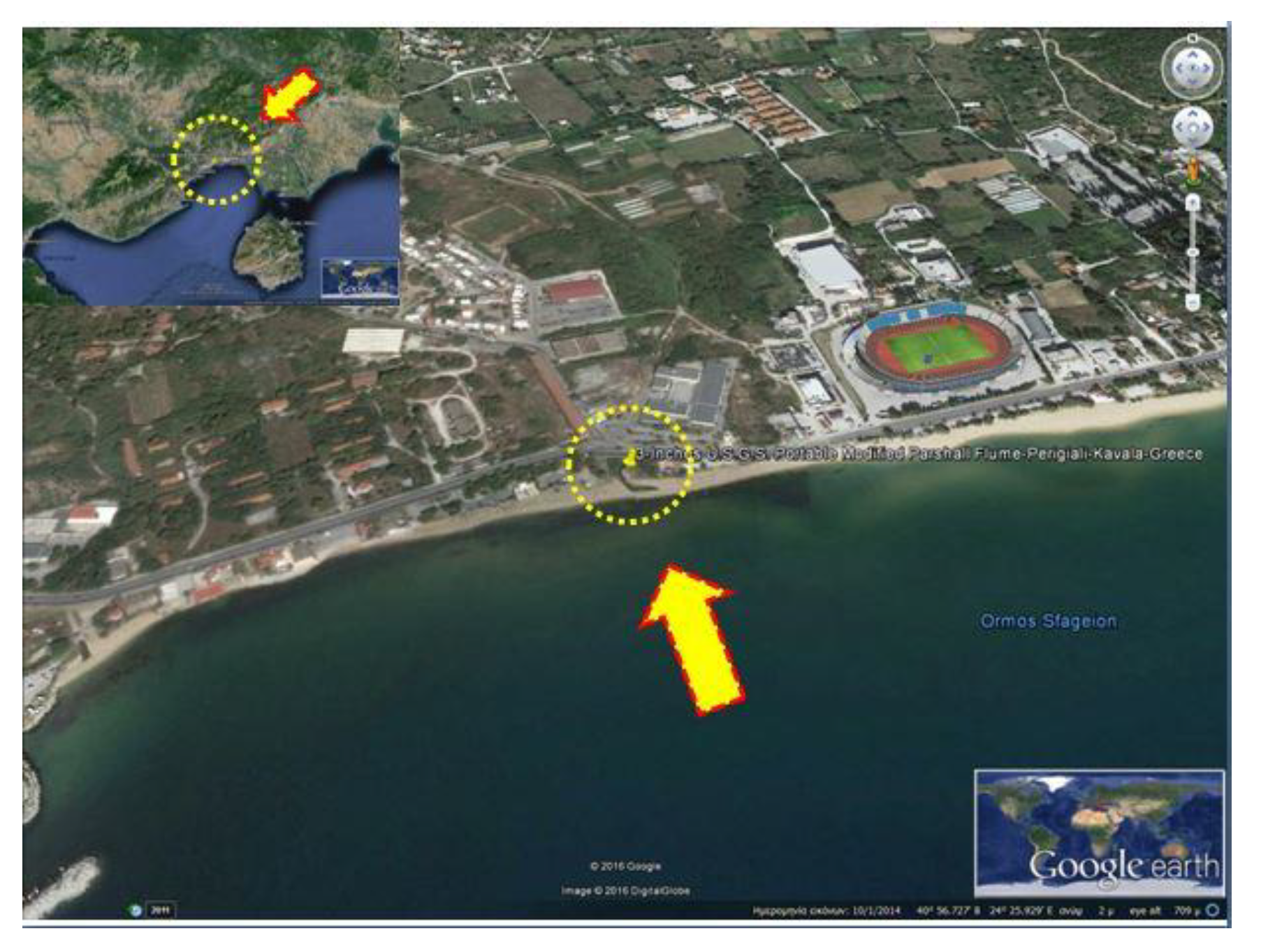
2. Study Area
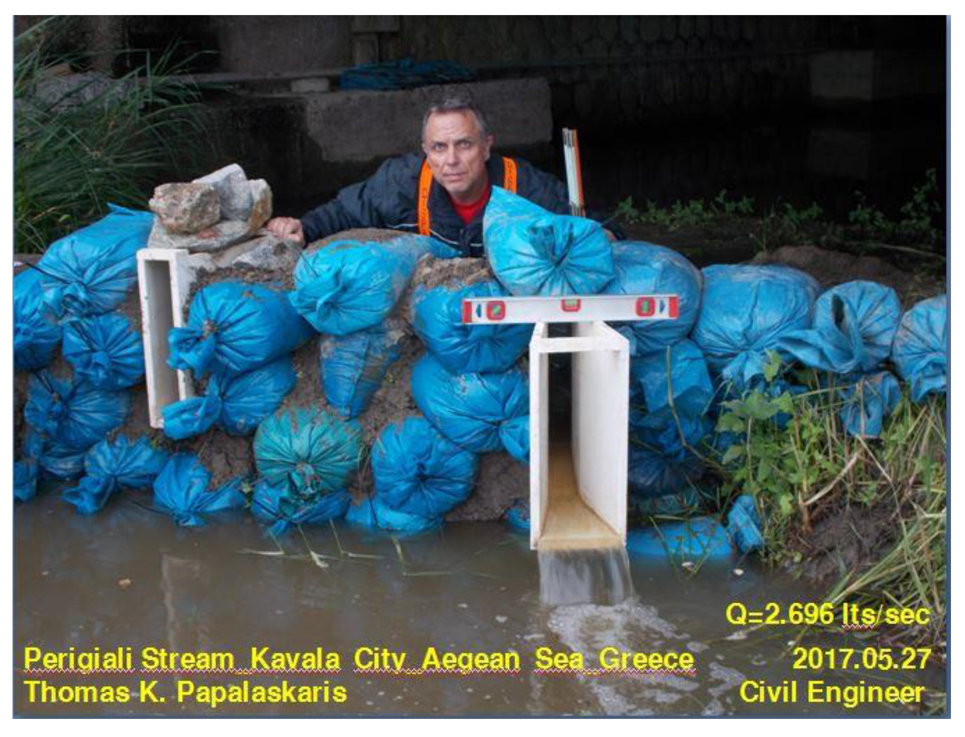
3. Materials and Methods
- Generating random values for each of the independent (meteorological) variables involved
- Introduce each different series of random values involved to arrive at a total daily low stream flow rate value (dependent variable “Y”)
- The anticipated daily low stream flow rate value is then considered the average resulted from these values.
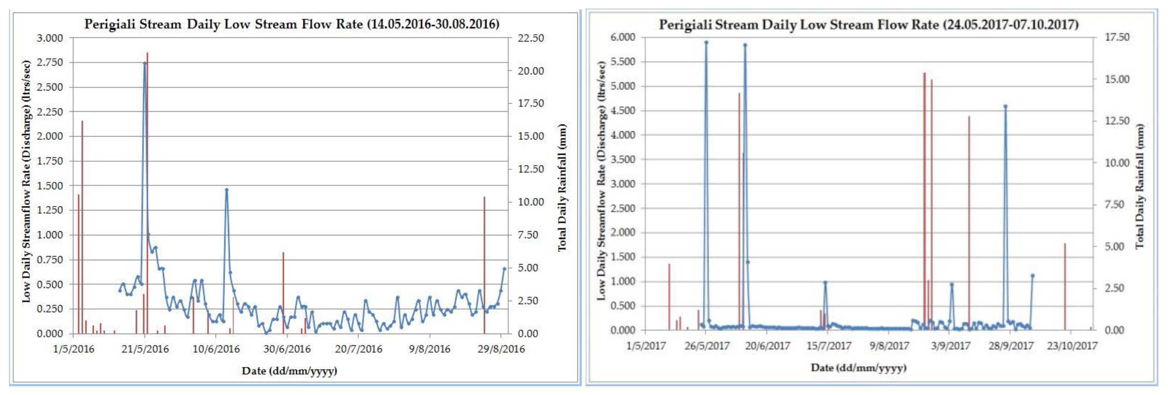
4. Results
5. Discussion and Conclusions
6. Further Research
Supplementary Materials
Author Contributions
Conflicts of Interest
Appendix A

| No. | Date | Stream Flow Rate (m3/s) Site-Measured |
|---|---|---|
| 1 | 14-5-2016 | 0.4370 |
| 2 | 15-5-2016 | 0.5080 |
| 3 | 16-5-2016 | 0.4030 |
| 4 | 17-5-2016 | 0.4030 |
| 5 | 18-5-2016 | 0.4720 |
| 6 | 19-5-2016 | 0.5830 |
| 7 | 20-5-2016 | 0.5080 |
| 8 | 21-5-2016 | 2.7460 |
| 9 | 22-5-2016 | 1.0110 |
| 10 | 23-5-2016 | 0.8300 |
| 11 | 24-5-2016 | 0.8740 |
| 12 | 25-5-2016 | 0.6620 |
| 13 | 26-5-2016 | 0.6620 |
| 14 | 27-5-2016 | 0.3700 |
| 15 | 28-5-2016 | 0.2488 |
| 16 | 29-5-2016 | 0.3701 |
| 17 | 30-5-2016 | 0.2775 |
| 18 | 31-5-2016 | 0.3381 |
| 19 | 1-6-2016 | 0.2488 |
| 20 | 2-6-2016 | 0.1700 |
| 21 | 3-6-2016 | 0.3701 |
| 22 | 4-6-2016 | 0.5451 |
| 23 | 5-6-2016 | 0.3381 |
| 24 | 6-6-2016 | 0.5450 |
| 25 | 7-6-2016 | 0.3072 |
| 26 | 8-6-2016 | 0.1950 |
| 27 | 9-6-2016 | 0.1238 |
| 28 | 10-6-2016 | 0.1238 |
| 29 | 11-6-2016 | 0.1950 |
| 30 | 12-6-2016 | 0.1238 |
| 31 | 13-6-2016 | 1.4650 |
| 32 | 14-6-2016 | 0.6220 |
| 33 | 15-6-2016 | 0.4371 |
| 34 | 16-6-2016 | 0.3072 |
| 35 | 17-6-2016 | 0.2213 |
| 36 | 18-6-2016 | 0.3072 |
| 37 | 19-6-2016 | 0.2775 |
| 38 | 20-6-2016 | 0.1950 |
| 39 | 21-6-2016 | 0.2775 |
| 40 | 22-6-2016 | 0.0832 |
| 41 | 23-6-2016 | 0.1028 |
| 42 | 24-6-2016 | 0.0115 |
| 43 | 25-6-2016 | 0.0344 |
| 44 | 26-6-2016 | 0.1462 |
| 45 | 27-6-2016 | 0.1462 |
| 46 | 28-6-2016 | 0.2775 |
| 47 | 29-6-2016 | 0.1700 |
| 48 | 30-6-2016 | 0.0652 |
| 49 | 1-7-2016 | 0.1700 |
| 50 | 2-7-2016 | 0.1700 |
| 51 | 3-7-2016 | 0.3701 |
| 52 | 4-7-2016 | 0.2775 |
| 53 | 5-7-2016 | 0.2775 |
| 54 | 6-7-2016 | 0.0652 |
| 55 | 7-7-2016 | 0.2213 |
| 56 | 8-7-2016 | 0.0218 |
| 57 | 9-7-2016 | 0.0832 |
| 58 | 10-7-2016 | 0.1028 |
| 59 | 11-7-2016 | 0.1028 |
| 60 | 12-7-2016 | 0.1028 |
| 61 | 13-7-2016 | 0.0489 |
| 62 | 14-7-2016 | 0.1238 |
| 63 | 15-7-2016 | 0.0652 |
| 64 | 16-7-2016 | 0.2213 |
| 65 | 17-7-2016 | 0.1462 |
| 66 | 18-7-2016 | 0.0344 |
| 67 | 19-7-2016 | 0.1950 |
| 68 | 20-7-2016 | 0.1028 |
| 69 | 21-7-2016 | 0.0344 |
| 70 | 22-7-2016 | 0.3381 |
| 71 | 23-7-2016 | 0.2213 |
| 72 | 24-7-2016 | 0.1950 |
| 73 | 25-7-2016 | 0.1238 |
| 74 | 26-7-2016 | 0.0340 |
| 75 | 27-7-2016 | 0.1028 |
| 76 | 28-7-2016 | 0.0489 |
| 77 | 29-7-2016 | 0.0832 |
| 78 | 30-7-2016 | 0.1238 |
| 79 | 31-7-2016 | 0.3701 |
| 80 | 1-8-2016 | 0.0652 |
| 81 | 2-8-2016 | 0.1950 |
| 82 | 3-8-2016 | 0.1028 |
| 83 | 4-8-2016 | 0.1462 |
| 84 | 5-8-2016 | 0.2488 |
| 85 | 6-8-2016 | 0.3381 |
| 86 | 7-8-2016 | 0.1238 |
| 87 | 8-8-2016 | 0.1950 |
| 88 | 9-8-2016 | 0.3701 |
| 89 | 10-8-2016 | 0.1950 |
| 90 | 11-8-2016 | 0.3381 |
| 91 | 12-8-2016 | 0.2488 |
| 92 | 13-8-2016 | 0.1950 |
| 93 | 14-8-2016 | 0.2488 |
| 94 | 15-8-2016 | 0.2219 |
| 95 | 16-8-2016 | 0.2775 |
| 96 | 17-8-2016 | 0.4371 |
| 97 | 18-8-2016 | 0.3701 |
| 98 | 19-8-2016 | 0.4031 |
| 99 | 20-8-2016 | 0.3072 |
| 100 | 21-8-2016 | 0.1950 |
| 101 | 22-8-2016 | 0.2213 |
| 102 | 23-8-2016 | 0.4371 |
| 103 | 24-8-2016 | 0.2775 |
| 104 | 25-8-2016 | 0.2213 |
| 105 | 26-8-2016 | 0.2775 |
| 106 | 27-8-2016 | 0.2775 |
| 107 | 28-8-2016 | 0.3072 |
| 108 | 29-8-2016 | 0.4371 |
| 109 | 30-8-2016 | 0.6616 |
| 110 | 24-5-2017 | 0.1210 |
| 111 | 25-5-2017 | 0.0820 |
| 112 | 26-5-2017 | 5.9150 |
| 113 | 27-5-2017 | 0.2130 |
| 114 | 28-5-2017 | 0.0820 |
| 115 | 29-5-2017 | 0.0650 |
| 116 | 30-5-2017 | 0.1010 |
| 117 | 31-5-2017 | 0.0490 |
| 118 | 1-6-2017 | 0.0340 |
| 119 | 2-6-2017 | 0.0650 |
| 120 | 3-6-2017 | 0.0650 |
| 121 | 4-6-2017 | 0.0820 |
| 122 | 5-6-2017 | 0.0650 |
| 123 | 6-6-2017 | 0.0820 |
| 124 | 7-6-2017 | 0.0650 |
| 125 | 8-6-2017 | 0.0820 |
| 126 | 9-6-2017 | 0.1010 |
| 127 | 10-6-2017 | 0.0820 |
| 128 | 11-6-2017 | 5.8560 |
| 129 | 12-6-2017 | 1.4010 |
| 130 | 13-6-2017 | 0.0650 |
| 131 | 14-6-2017 | 0.1010 |
| 132 | 15-6-2017 | 0.0820 |
| 133 | 16-6-2017 | 0.0820 |
| 134 | 17-6-2017 | 0.1010 |
| 135 | 18-6-2017 | 0.0820 |
| 136 | 19-6-2017 | 0.0650 |
| 137 | 20-6-2017 | 0.0650 |
| 138 | 21-6-2017 | 0.0650 |
| 139 | 22-6-2017 | 0.0650 |
| 140 | 23-6-2017 | 0.0650 |
| 141 | 24-6-2017 | 0.0490 |
| 142 | 25-6-2017 | 0.0650 |
| 143 | 26-6-2017 | 0.0490 |
| 144 | 27-6-2017 | 0.0490 |
| 145 | 28-6-2017 | 0.0490 |
| 146 | 29-6-2017 | 0.0490 |
| 147 | 30-6-2017 | 0.0490 |
| 148 | 1-7-2017 | 0.0490 |
| 149 | 2-7-2017 | 0.0490 |
| 150 | 3-7-2017 | 0.0645 |
| 151 | 4-7-2017 | 0.0486 |
| 152 | 5-7-2017 | 0.0486 |
| 153 | 6-7-2017 | 0.0486 |
| 154 | 7-7-2017 | 0.0486 |
| 155 | 8-7-2017 | 0.0486 |
| 156 | 9-7-2017 | 0.0486 |
| 157 | 10-7-2017 | 0.0344 |
| 158 | 11-7-2017 | 0.0344 |
| 159 | 12-7-2017 | 0.0645 |
| 160 | 13-7-2017 | 0.0344 |
| 161 | 14-7-2017 | 0.9872 |
| 162 | 15-7-2017 | 0.1007 |
| 163 | 16-7-2017 | 0.0819 |
| 164 | 17-7-2017 | 0.1421 |
| 165 | 18-7-2017 | 0.1208 |
| 166 | 19-7-2017 | 0.1007 |
| 167 | 20-7-2017 | 0.0819 |
| 168 | 21-7-2017 | 0.0486 |
| 169 | 22-7-2017 | 0.0645 |
| 170 | 23-7-2017 | 0.0645 |
| 171 | 24-7-2017 | 0.0645 |
| 172 | 25-7-2017 | 0.0344 |
| 173 | 26-7-2017 | 0.0486 |
| 174 | 27-7-2017 | 0.0486 |
| 175 | 28-7-2017 | 0.0486 |
| 176 | 29-7-2017 | 0.0486 |
| 177 | 30-7-2017 | 0.0486 |
| 178 | 31-7-2017 | 0.0486 |
| 179 | 1-8-2017 | 0.0344 |
| 180 | 2-8-2017 | 0.0344 |
| 181 | 3-8-2017 | 0.0344 |
| 182 | 4-8-2017 | 0.0344 |
| 183 | 5-8-2017 | 0.0344 |
| 184 | 6-8-2017 | 0.0486 |
| 185 | 7-8-2017 | 0.0344 |
| 186 | 8-8-2017 | 0.0344 |
| 187 | 9-8-2017 | 0.0344 |
| 188 | 10-8-2017 | 0.0344 |
| 189 | 11-8-2017 | 0.0344 |
| 190 | 12-8-2017 | 0.0344 |
| 191 | 13-8-2017 | 0.0344 |
| 192 | 14-8-2017 | 0.0344 |
| 193 | 15-8-2017 | 0.0344 |
| 194 | 16-8-2017 | 0.0344 |
| 195 | 17-8-2017 | 0.0344 |
| 196 | 18-8-2017 | 0.0221 |
| 197 | 19-8-2017 | 0.2060 |
| 198 | 20-8-2017 | 0.1890 |
| 199 | 21-8-2017 | 0.1670 |
| 200 | 22-8-2017 | 0.0486 |
| 201 | 23-8-2017 | 0.1210 |
| 202 | 24-8-2017 | 0.0486 |
| 203 | 25-8-2017 | 0.0486 |
| 204 | 26-8-2017 | 0.2070 |
| 205 | 27-8-2017 | 0.1690 |
| 206 | 28-8-2017 | 0.0344 |
| 207 | 29-8-2017 | 0.0486 |
| 208 | 30-8-2017 | 0.1770 |
| 209 | 31-8-2017 | 0.1710 |
| 210 | 1-9-2017 | 0.0730 |
| 211 | 2-9-2017 | 0.0470 |
| 212 | 3-9-2017 | 0.1930 |
| 213 | 4-9-2017 | 0.9439 |
| 214 | 5-9-2017 | 0.0344 |
| 215 | 6-9-2017 | 0.0360 |
| 216 | 7-9-2017 | 0.0320 |
| 217 | 8-9-2017 | 0.0430 |
| 218 | 9-9-2017 | 0.1390 |
| 219 | 10-9-2017 | 0.1370 |
| 220 | 11-9-2017 | 0.0220 |
| 221 | 12-9-2017 | 0.0344 |
| 222 | 13-9-2017 | 0.1450 |
| 223 | 14-9-2017 | 0.0344 |
| 224 | 15-9-2017 | 0.1610 |
| 225 | 16-9-2017 | 0.1490 |
| 226 | 17-9-2017 | 0.0486 |
| 227 | 18-9-2017 | 0.1080 |
| 228 | 19-9-2017 | 0.0486 |
| 229 | 20-9-2017 | 0.0344 |
| 230 | 21-9-2017 | 0.0990 |
| 231 | 22-9-2017 | 0.0714 |
| 232 | 23-9-2017 | 0.1380 |
| 233 | 24-9-2017 | 0.0996 |
| 234 | 25-9-2017 | 0.0934 |
| 235 | 26-9-2017 | 4.6003 |
| 236 | 27-9-2017 | 0.1870 |
| 237 | 28-9-2017 | 0.1510 |
| 238 | 29-9-2017 | 0.1790 |
| 239 | 30-9-2017 | 0.0330 |
| 240 | 1-10-2017 | 0.1280 |
| 241 | 2-10-2017 | 0.1420 |
| 242 | 3-10-2017 | 0.0910 |
| 243 | 4-10-2017 | 0.0650 |
| 244 | 5-10-2017 | 0.1050 |
| 245 | 6-10-2017 | 0.0590 |
| 246 | 7-10-2017 | 1.1245 |
References
- Gustard, A.; Demuth, S. Estimating, Predicting and Forecasting Low Flows. In Manual on Low-Flow Estimation and Prediction (Operational Hydrology Report No. 50), 1st ed.; Gustard, A., Demuth, S., Eds.; World Meteorological Organization (WMO): Geneva, Switzerland, 2008; Volume 1029, pp. 16–21. [Google Scholar]
- Papalaskaris, T.; Panagiotidis, T. Artificial Low Stream Flow Time Series Generation of Perigiali Stream, Kavala city, NE Greece. In Proceedings of the 6th International Symposium on Environmental & Material Flow Management (6th E.M.F.M.), Bor, Serbia, 2–4 October 2016; dr Živan, Ž., dr Ivan, M., dr Predrag, D., Eds.; University of Belgrade, Technical Faculty in Bor: Bor, Serbia, 2016; pp. 20–38. [Google Scholar]
- Papalaskaris, T.; Panagiotidis, T. Stochastic generation of low stream flow data of Perigiali Stream, Kavala city, NE Greece. In Proceedings of the 10th World Congress of European Water Resources Association (“E.W.R.A.”) on Water Resources and Environment “Panta Rhei” 2017 (10th “E.W.R.A.” “Panta Rhei” 2017), Athens, Greece, 5–9 July 2017; George, T., Vassilios, T., Harris, V., Dimitris, T., Eds.; European Water Resources Association (E.W.R.A.): Athens, Greece, 2017; pp. 953–960. [Google Scholar]
- Papalaskaris, T.; Panagiotidis, T. Stochastic generation of low stream flow data of Perigiali Stream, Kavala city, NE Greece. Eur. Water 2017, 60, 299–306. Available online: http://ewra.net/ew/pdf/EW_2017_60_41.pdf (accessed on 3 March 2018). [CrossRef]
- Papalaskaris, T.; Panagiotidis, T. Artificial low stream flow time series generation of Palaia Kavala Stream, Kavala City, NE Greece. In Proceedings of the 15th International Conference on Environmental Science & Technology 2017 (15th C.E.S.T. 2017), Rhodes Island, Greece, 31 August–2 September 2017; Lekkas, D.F., Ed.; cest2017_00842. Global Network for Environmental Science & Technology (Global-NEST), University of the Aegean: Athens, Greece, 2017. [Google Scholar]
- Monte Carlo Method. Available online: https://en.wikipedia.org/wiki/Monte_Carlo_method (accessed on 3 March 2018).
- Koutsoyiannis, D. A Monte Carlo approach to water management (invited). In Proceedings of the European Geosciences Union General Assembly, Vienna, Austria, 22–27 April 2012; Geophysical Research Abstracts: Vienna Austria, 2012; Volume 14, 3509, pp. 1–45. [Google Scholar]
- Flores, G. A Stochastic Model for Sewer Base Flows Using Monte Carlo Simulation. Master’s Thesis, Stellenbosch University, Faculty of Engineering, Department of Civil Engineering, Stellenbosch, South Africa, March 2015. [Google Scholar]
- Paisley, L.G.; Karlsen, E.; Jarp, J.; Mo, T.A. A Monte Carlo Simulation Model for Assessing the Risk of Introduction of Gyrodactylus Salaries to the Tana River, Norway. Dis. Aquat. Org. 1999, 37, 145–152. Available online: http://www.int-res.com/abstracts/dao/v37/n2/p145-152/ (accessed on 3 March 2018). [CrossRef] [PubMed]
- Johnson, A. Modified Parshall Flume (U.S. Geological Survey Open-File Report), 1st ed.; United States Department of the Interior Geological Survey: Denver, CO, USA, 1963; pp. 1–8. [Google Scholar]
- Rantz, S.E.; Barnes, H.H.; Carter, R.W.; Smoot, G.F.; Matthai, H.F.; Pendleton, A.F.; Hulsing, H.; Bodhaine, G.L.; Davidian, J.; Buchanan, T.J.; et al. Measurement of Discharge by Miscellaneous Methods. In Measurement and Computation of Streamflow: Volume 1. Measurement of Stage and Discharge, 1st ed.; United States Government Printing Office: Washington, DC, USA, 1982; Volume 1, pp. 260–272. [Google Scholar]
- Modified Parshall Flume-(U.S.G.S.). Available online: https://www.usgs.gov/media/images/modified-parshall-flume (accessed on 3 March 2018).
- U.S.G.S. Portable Parshall Flume (Open-Channel-Flow Hydrological Equipment). Available online: https://www.openchannelflow.com/blog/usgs-portable-parshall-flume (accessed on 3 March 2018).
- U.S.G.S. Portable Parshall Flume, 3in (Rickly Hydrological Equipment). Available online: http://rickly.com/usgs-portable-parshall-flume-3in/ (accessed on 3 March 2018).
- Measuring Low Flow in San Pedro River. Available online: https://www.youtube.com/watch?v=gLWtfMYicrI (accessed on 3 March 2018).
- Inspecting a Parshall Flume (3-Inch USGS Modified Portable). Available online: https://www.youtube.com/watch?v=YtqflgfOb5E (accessed on 3 March 2018).
- Inspecting a Parshall Flume. Available online: https://www.youtube.com/watch?v=y6hiOLgTo6g (accessed on 3 March 2018).
- Inspecting a Parshall Flume (a+b). Available online: https://www.youtube.com/watch?v=EgV5AKAYBe4 (accessed on 3 March 2018).
- MSc. In Management of Water Resources in the Mediterranean 3. Available online: https://www.youtube.com/watch?v=picUMHITkx0 (accessed on 3 March 2018).
- Father of the Flume: Ralph Parshall. Available online: https://lib2.colostate.edu/archives/water/parshall/ (accessed on 3 March 2018).
- Papalaskaris, T.; Dimitriadou, P. Artificial Neural Network for Bed Load Transport Rate in Nestos River, Greece. Spec. Top. Rev. Porous Media 2017, 8, 145–157. Available online: http://www.dl.begellhouse.com/journals/3d21681c18f5b5e7,0e5e7d7c2836d626,2a6142094c2e98ac.html (accessed on 3 March 2018). [CrossRef]


| Number of Iterations | Expected Daily Low Stream Flow Rate (Mean) | Median | Standard Deviation | True (Reviewed) Error of the Estimate | Kurtosis | Skewness |
|---|---|---|---|---|---|---|
| 2138 | 2.596 | 2.614 | 1.858 | 0.121 (4.644%) | −0.383 | 0.017 |
Publisher’s Note: MDPI stays neutral with regard to jurisdictional claims in published maps and institutional affiliations. |
© 2018 by the authors. Licensee MDPI, Basel, Switzerland. This article is an open access article distributed under the terms and conditions of the Creative Commons Attribution (CC BY) license (https://creativecommons.org/licenses/by/4.0/).
Share and Cite
Papalaskaris, T.; Panagiotidis, T. Forecasting Low Stream Flow Rate Using Monte—Carlo Simulation of Perigiali Stream, Kavala City, NE Greece. Proceedings 2018, 2, 580. https://doi.org/10.3390/proceedings2110580
Papalaskaris T, Panagiotidis T. Forecasting Low Stream Flow Rate Using Monte—Carlo Simulation of Perigiali Stream, Kavala City, NE Greece. Proceedings. 2018; 2(11):580. https://doi.org/10.3390/proceedings2110580
Chicago/Turabian StylePapalaskaris, Thomas, and Theologos Panagiotidis. 2018. "Forecasting Low Stream Flow Rate Using Monte—Carlo Simulation of Perigiali Stream, Kavala City, NE Greece" Proceedings 2, no. 11: 580. https://doi.org/10.3390/proceedings2110580
APA StylePapalaskaris, T., & Panagiotidis, T. (2018). Forecasting Low Stream Flow Rate Using Monte—Carlo Simulation of Perigiali Stream, Kavala City, NE Greece. Proceedings, 2(11), 580. https://doi.org/10.3390/proceedings2110580