Article

A Fractional Computer Virus Propagation Model with Saturation Effect

1
Department of Computer Science, Sichuan University Jinjiang College, Meishan 620860, China
2
School of Big Data and Software Engineering, Chongqing University, Chongqing 400044, China
3
School of Information Technology, Deakin University, Melbourne, VIC 3125, Australia
*
Author to whom correspondence should be addressed.
Fractal Fract. 2025, 9(9), 587; https://doi.org/10.3390/fractalfract9090587
Submission received: 26 July 2025 / Revised: 24 August 2025 / Accepted: 2 September 2025 / Published: 4 September 2025

Abstract

The epidemic modeling of computer virus propagation is identified as an effective approach to understanding the mechanism of virus spread. Fraction-order virus spread models exhibit remarkable advantages over their integer-order counterparts. Based on a type of bursting virus, a fractional computer virus propagation model with saturation effect is suggested. The basic properties of the model are discussed. The basic reproduction number of the model is determined. The virus–endemic equilibria of the model are determined. A criterion for the global asymptotic stability of the virus-free equilibrium is derived. For a pair of potential virus–endemic equilibria, criteria for the local asymptotic stability are presented. Some interesting properties of the model, ranging from the impact of the fractional order and the saturation index on virus spread to their coupling effect, are revealed through numerical simulations. This work helps gain a deep insight into the laws governing virus propagation.

1. Introduction

A computer virus is a type of malicious software designed to replicate itself. Once activated, it can spread from one computer to another, with the intent of performing malicious operations such as disrupting systems, corrupting data, and stealing information [1]. Computer viruses pose huge threats to several areas such as network security and digital asset protection. For example, in 2025, a large-scale hospital was attacked by the Medusa ransomware. The attackers took advantage of the unpatched Microsoft system vulnerabilities in the hospital, spread the virus through remote-control tools, encrypted about 50 TB of medical data, and demanded a ransom of RMB 110 million [2]. Consequently, the issue of defending against electronic viruses is a long-standing research hotspot in the domain of cybersecurity.
The mathematical modeling of biological infectious diseases has a history of nearly a hundred years [3]. Inspired by the high degree of similarity between digital viruses and infectious diseases, Kepart and White [4,5] proposed the earliest computer virus propagation models (See [6] for a recent review of virus propagation models). The research on virus spread models hold significant value for several reasons: (1) The way a virus spreads across networks over time can be predicted, enabling proactive preparation for potential outbreaks and resource allocation. (2) Various countermeasures (e.g., patch distribution and quarantine protocols) can be tested in a simulation environment, identifying the most effective ways to contain or mitigate infections. (3) More resilient network architectures and security mechanisms can be developed by gaining insights from propagation models, reducing susceptibility to viral attacks.
In most existing computer virus spread models, the infection rate takes the form of bilinear interaction. Due to the following reasons, the bilinear pattern significantly overestimates real-world infection rates: (1) It is unrealistically assumed that every infected device can connect with every susceptible one uniformly. In reality, network structures restrict interactions, reducing actual transmission opportunities. (2) Real-time defenses (antivirus updates, quarantines, user blocking actions, etc.) that lower effective transmission rates are rarely accounted for. (3) Varying security levels and user behavior create uneven susceptibility, making spread less efficient than the model predicts. For the purpose of accurately fitting the realistic infection rate, a spectrum of computer virus propagation models with a nonlinear infection rate have been suggested. In these models, the infection rate is of the form β S I 1 + θ I [7], the form β S I 1 + θ S [8,9], the form β S I 1 + θ ( S + I ) [10,11,12], the form β S I 1 + θ 1 S + θ 2 I [13], the form β S I 1 + θ I 2 [14,15], or the form β S f ( I ) [16].
A fractional-order dynamical system is a type of mathematical framework used to describe the evolution of complex systems over time. where the dynamics are governed by fractional calculus [17]. Unlike classical integer-order dynamical systems, fractional-order systems account for memory effects of the system. This means that the current state of the system depends not only on its immediate past but also on its entire history, making it more suitable for modeling real-world phenomena with long-range dependency. In the past decade, fractional virus spread models have received considerable interest. Ref. [18] showed the existence, uniqueness, and Hyers–Ulam stability of a solution to a fractional model. Ref. [19], the authors studied a fractional model with kill signals through numerical simulations. Ref. [20] examined the asymptotic stability of a fractional model. Refs. [21,22] inspected the asymptotic stability of a pair of fractional models and presented criteria for the existence of Hopf bifurcation. In these models, the outbreak time of a virus will be later than predicted by integer-order models, and the propagation peak will be delayed. Additionally, unlike the abrupt changes in propagation rate in integer-order models, the change in virus propagation rate in fractional-order models is gentler. It can better reflect the gradual process of actual virus propagation affected by various factors (such as network topology and protective measures).
In real-world scenarios, most computer viruses are designed to enter a state of viral latency before outbreak, with the intent of infecting as many susceptible nodes as possible. In this context, it is proper to characterize the propagation process of a virus by means of a Susceptible-Latent-Bursting-Susceptible (SLBS) model, where ’susceptible’ represents the state of not being infected with a virus; ‘latent’ represents the state of being infected with a propagating virus, but not performing virus-induced destructive operations; ‘bursting’ describes the state of being infected with a propagation virus and performing virus-induced destructive operations; and the transition from the latent state to the bursting state represents a virus in latency that starts performing malicious operations other than infections (see [23,24,25] for ordinary SLBS models and [26,27,28] for delayed SLBS models). Later, some variants of the SLBS models, which are known as the Susceptible-Latent-Bursting-Recovered-Susceptible (SLBRS) models, have been advised [29,30,31]. In an SLBRS model, an added state known as ‘recovered’ is accounted for to reflect the repair of outbreak nodes.
In the framework of SLBS viruses, this article advises a Caputo fractional computer virus propagation model with a nonlinear saturation infection rate. Our work is closely related to that of [25], where a generic nonlinear infection rate is assumed; the work is conducted on an integer-order virus spread model. In our article, the well-known Holling type II saturation infection rate is introduced, and the model is extended to the situation of fraction-order virus propagation.
The subsequent materials of this article are organized as follows: Section 2 provides basic notations and terminologies. Section 3 formulates the virus propagation model. Section 4 discusses the basic properties of the model. Section 5 figures out the basic reproduction number of the model. Section 6 determines the virus–endemic equilibria of the model. Section 7 gives a criterion for the global asymptotic stability of the virus-free equilibrium. Section 8 derives a criterion for the local asymptotic stability of the virus–endemic equilibrium with no latent component. Section 9 reports a criterion for the local asymptotic stability of the virus–endemic equilibrium with a non-zero latent component. Section 10 validates the theoretical findings through numerical simulations. Section 11 conducts further discussions. This work is summarized in Section 12.

2. Notations and Terminologies

This section introduces the basic notations and terminologies that will be used in the subsequent research.
Definition 1.
The Mittag-Leffler function with parameter α 0 is defined as follows:
E α ( z ) = k = 0 z k Γ ( α k + 1 ) .
The Mittag-Leffler function with parameters α 0 and β 0 is defined as follows:
E α , β ( z ) = k = 0 z k Γ ( α k + β ) .
Here, Γ ( · ) represents the Gamma function.
Definition 2.
Let 0 < α < 1 . The α-order Caputo derivative of the function f is defined as follows:
D α f ( t ) = 1 Γ ( 1 α ) 0 t f ( s ) ( t s ) α d s .
Lemma 1
([17]). Let 0 < α < 1 , x : [ 0 , ) R n , f : [ 0 , ) × R n R n . Consider the following fractional differential equation:
D α x ( t ) = f ( t , x ( t ) ) , x ( 0 ) = x 0 .
Suppose the following conditions are met:
(C1) 
f is continuous in the region [ 0 , ) × R n .
(C2) 
f is globally Lipschitz continuous with respect to x, i.e., there exists a positive constant C such that the following is true:
  f ( t , x 1 ) f ( t , x 2 ) C x 1 x 2 , x 1 , x 2 R n .
Then, Equation (4) admits a unique solution.
Lemma 2
([17]). Let 0 < α < 1 , x : [ 0 , ) R n , A is a real matrix of order n, { λ 1 , , λ n } denotes the spectrum of A. Consider the following linear fractional differential equation:
D α x ( t ) = A x ( t ) .
The following assertions hold:
(A1) 
Suppose all λ i meet | arg ( λ i ) | > α π 2 . Then, the origin is locally asymptotically stable.
(A2) 
Suppose there exists λ i such that | arg ( λ i ) | < α π 2 . Then, the origin is unstable.
Lemma 3
([17]). Let 0 < α < 1 , a , b > 0 . Suppose D α x ( t ) = a b x ( t ) , t 0 . Then, the following is true:
x ( t ) = a b + x ( 0 ) a b E α ( b t α ) .
Lemma 4
([17]). Let 0 < α < 1 , c > 0 . Suppose D α x ( t ) c x ( t ) , t 0 . Then, the following is true:
x ( t ) x ( 0 ) E α ( c t α ) .

3. A Fractional Computer Virus Propagation Model

Consider an organization (an enterprise, a research institute, a government sector, etc.). Suppose the computers in the organization are interconnected by a group of computers to form an intranet. For brevity, all computers within the network are referred to as internal, whereas all computers outside the network are referred to as external. Owing to different reasons, every internal computer may possibly be physically disconnected from the network to become a part outside the intranet, whereas every external computer may possibly be physically connected to the network to become a part of the intranet.
Under the threat of a specific virus, assume (a) every internal computer is either susceptible (not infected with the virus), latent (infected with the virus and performing infection operations only), or bursting (infected with the virus and performing malicious operations including infections); (b) every external computer is susceptible. Let S ( t ) (resp. L ( t ) , B ( t ) ) denote the number of susceptible (resp. latent, bursting) internal computers at time t. The following assumptions are introduced:
( A 1 )
External computers are physically connected to the network at constant rate μ > 0 (entrance rate).
( A 2 )
Every internal computer is physically disconnected from the network at constant rate δ > 0 (exit rate).
( A 3 )
When contacting with latent computers, susceptible internal computers become infected, do not perform virus-induced destructive operations, and hence become latent at time t at rate β S ( t ) L ( t ) 1 + σ [ L ( t ) + B ( t ) ] . Here, the constant β > 0 is referred to as the infection force, while the constant σ > 0 is referred to as the saturation index.
( A 4 )
When contacting with bursting computers, susceptible internal computers become infected, perform virus-induced destructive operations, and hence become bursting at time t at rate β S ( t ) B ( t ) 1 + σ [ L ( t ) + B ( t ) ] .
( A 5 )
Due to transition from latency to burst, every latent computer becomes bursting at rate η > 0 (burst rate).
( A 6 )
Due to recovery from burst, every bursting computer becomes susceptible at rate γ > 0 (recovery rate).
( A 7 )
Let α denote the order of the Caputo derivative used in the subsequent modeling. Assume 0 < α < 1 .
The above assumptions lead to the following fractional computer virus propagation model:
D α S ( t ) = μ β S ( t ) [ L ( t ) + B ( t ) ] 1 + σ [ L ( t ) + B ( t ) ] + γ B ( t ) δ S ( t ) , t 0 , D α L ( t ) = β S ( t ) L ( t ) 1 + σ [ L ( t ) + B ( t ) ] η L ( t ) δ L ( t ) , t 0 , D α B ( t ) = β S ( t ) B ( t ) 1 + σ [ L ( t ) + B ( t ) ] + η L ( t ) γ B ( t ) δ B ( t ) , t 0 , S ( 0 ) 0 , L ( 0 ) 0 , B ( 0 ) 0 .
Remark 1.
The first and main approach to establishing a fractional compartment model is by directly introducing a fractional-order derivative to yield the fractional model (not by simply replacing the regular derivative in a compartment model with a fractional-order derivative to yield the fractional model). A so-constructed fractional model has a striking advantage—in parallel to its integer-order counterpart, the dynamics of the model can be investigated theoretically, yielding rich conclusions. Consequently, most existing fractional compartment models, including model (9), are constructed in this way. In the research of such a fractional model, the units of all the associated rates may be uniformly set as 1 t i m e α . As a result, both sides of the model have the same unit.
Remark 2.
The second approach to establishing a fractional compartment model is by introducing a stochastic process to derive the fractional model [32,33]. A so-constructed fractional model is typically explainable, with the disadvantage of being highly complex and difficult for theoretical research.

4. Basic Properties

This section examines the basic properties of the solution to the model (9). First, inspect the non-negativity of the solution.
Lemma 5.
Consider the model (9). Then, S ( t ) 0 , L ( t ) 0 , B ( t ) 0 , t 0 .
Proof of Lemma 5.
On the contrary, suppose there exists t 1 > 0 such that (a) S ( t ) 0 , L ( t ) 0 , B ( t ) 0 , 0 t < t 1 , (b) S ( t 1 ) < 0 , L ( t 1 ) < 0 , or B ( t 1 ) < 0 . Consider the following three possibilities.
Case 1:  S ( t 1 ) < 0 . It follows from the first equation of Equation (9) that the following is true:
D α S ( t ) = μ β S ( t ) [ L ( t ) + B ( t ) ] 1 + σ [ L ( t ) + B ( t ) ] + γ B ( t ) δ S ( t ) β S ( t ) [ L ( t ) + B ( t ) ] 1 + σ [ L ( t ) + B ( t ) ] δ S ( t ) , 0 t < t 1 .
Let
f ( x ) = x 1 + σ x , x 0 .
Then,
f ( x ) = 1 ( 1 + σ x ) 2 > 0 , x 0 .
So,
f ( x ) < f ( + ) = 1 σ , x 0 .
Thus,
f ( L ( t ) + B ( t ) ) = L ( t ) + B ( t ) 1 + σ [ L ( t ) + B ( t ) ] < 1 σ , 0 t < t 1 .
Hence, it follows from Equation (10) that the following is true:
D α S ( t ) β σ + δ S ( t ) , 0 t < t 1 .
It follows from Lemma 4 that the following is true:
S ( t ) S ( 0 ) E α β σ + δ t α , 0 t < t 1 .
Hence,
S ( t 1 ) = lim S ( t 1 ) S ( 0 ) E α β σ + δ t 1 α 0 .
This contradicts the assumption of S ( t 1 ) < 0 .
Case 2:  L ( t 1 ) < 0 . It follows from the second equation of Equation (9) that the following is true:
D α L ( t ) = β S ( t ) L ( t ) 1 + σ [ L ( t ) + B ( t ) ] η L ( t ) δ L ( t ) ( η + δ ) L ( t ) , 0 t < t 1 .
It follows from Lemma 4 that the following is true:
L ( t ) L ( 0 ) E α ( ( η + δ ) t α ) , 0 t < t 1 .
Hence,
L ( t 1 ) = lim L ( t 1 ) L ( 0 ) E α ( ( η + δ ) t 1 α ) 0 .
This contradicts the assumption of L ( t 1 ) < 0 .
Case 3:  B ( t 1 ) < 0 . It follows from the third equation of Equation (9) that the following is true:
D α B ( t ) = β S ( t ) B ( t ) 1 + σ [ L ( t ) + B ( t ) ] + α L ( t ) γ B ( t ) δ B ( t ) ( γ + δ ) L ( t ) , 0 t < t 1 .
It follows from Lemma 4 that the following is true:
B ( t ) B ( 0 ) E α ( ( γ + δ ) t α ) , 0 t < t 1 .
Hence,
B ( t 1 ) = lim B ( t 1 ) = B ( 0 ) E α ( ( γ + δ ) t 1 α ) 0 .
This contradicts the assumption of L ( t 1 ) < 0 .
The assertion holds based on the principle of reduction to absurdity. □
Second, inspect the boundedness of the solution.
Lemma 6.
The solution to model (9) is bounded.
Proof of Lemma 6.
Let N ( t ) = S ( t ) + I ( t ) + R ( t ) denote the total number of internal nodes at time t. Adding the three equations in model (9) yields the following:
D α N ( t ) = μ δ N ( t ) , t 0 .
So,
N ( t ) = μ δ + N ( 0 ) μ δ E α ( δ t α ) , t 0 ,
Notice that 0 E α ( δ t α ) 1 . It follows that:
N ( t ) = μ δ + N ( 0 ) μ δ E α ( δ t α ) μ δ + N ( 0 ) μ δ E α ( δ t α ) μ δ + N ( 0 ) μ δ = M .
In view of Lemma 5, the solution to the model (9) is bounded by the following set:
Ω = ( S , L , B ) R + 3 : S + L + B M .
Finally, examine the existence and uniqueness of the solution.
Lemma 7.
The solution to model (9) is existent and unique.
The proof of this lemma is shown in Appendix A.
It follows from Equation (9) that N ( t ) μ δ . Hence, the plane S + L + B = μ δ is an invariant manifold of model (9) that is attracting in the first octant. According to [34,35], it follows that model (9) can be reduced to the following model:
D α L ( t ) = β [ μ δ L ( t ) B ( t ) ] L ( t ) 1 + σ [ L ( t ) + B ( t ) ] η L ( t ) δ L ( t ) , D α B ( t ) = β [ μ δ L ( t ) B ( t ) ] B ( t ) 1 + σ [ L ( t ) + B ( t ) ] + η L ( t ) γ B ( t ) δ B ( t ) , t 0 .
In what follows, this model will be the focus of attention.

5. Basic Reproduction Number

Now, consider the basic reproduction number of model (28).
Theorem 1.
Let
R 1 = β μ δ ( η + δ ) , R 2 = β μ δ ( γ + δ ) .
The basic reproduction number of model (28) equals the following:
R 0 = max ( R 1 , R 2 ) .
Proof of Theorem 1.
Let F 1 ( t ) (resp. F 2 ( t ) ) denote the rate of appearance of new latent (bursting) nodes at time t, V 1 ( t ) (resp. V 2 ( t ) ) denote the rate of transfer of nodes out of the latent (resp. bursting) compartment at time t, and V 1 + ( t ) (resp. V 2 + ( t ) ) denote the rate of transfer of nodes into the latent (resp. bursting) compartment by all other means at time t. Then, the following is true:
F 1 ( t ) = β [ μ δ L ( t ) B ( t ) ] L ( t ) 1 + σ [ L ( t ) + B ( t ) ] , F 2 ( t ) = β [ μ δ L ( t ) B ( t ) ] B ( t ) 1 + σ [ L ( t ) + B ( t ) ] ,
V 1 ( t ) = η L ( t ) + δ L ( t ) , V 2 ( t ) = γ B ( t ) + δ B ( t ) ,
V 1 + ( t ) = 0 , V 2 + ( t ) = η L ( t ) .
Let
V 1 ( t ) = V 1 ( t ) V 1 + ( t ) = η L ( t ) + δ L ( t ) ,
V 2 ( t ) = V 2 ( t ) V 2 + ( t ) = γ B ( t ) + δ B ( t ) η L ( t ) .
Then,
D α L ( t ) = F 1 ( t ) V 1 ( t ) , D α B ( t ) = F 2 ( t ) V 2 ( t ) .
Let
F ( t ) = ( F 1 ( t ) , F 2 ( t ) ) T , V ( t ) = ( V 1 ( t ) , V 2 ( t ) ) T .
Let E 0 = ( 0 , 0 ) . Let D F ( t ) (resp. D V ( t ) ) denote the Jacobian matrix of F ( t ) (resp. V ( t ) ). Let F = D F ( t ) | E 0 (resp. V = D V ( t ) | E 0 ) denote the D F ( t ) (resp. D V ( t ) ) evaluated at E 0 . Then, the following is true:
F = F 1 ( t ) L ( t ) | E 0 F 1 ( t ) B ( t ) | E 0 F 2 ( t ) L ( t ) | E 0 F 2 ( t ) B ( t ) | E 0 = β μ δ 0 0 β μ δ .
V = V 1 ( t ) L ( t ) | E 0 V 1 ( t ) B ( t ) | E 0 V 2 ( t ) L ( t ) | E 0 V 2 ( t ) B ( t ) | E 0 = η + δ 0 η γ + δ .
So,
F V 1 = β μ δ 0 0 β μ δ η + δ 0 η γ + δ 1 = β μ δ 1 η + δ 0 1 ( γ + δ ) ( η + δ ) 1 γ + δ ,
which admits the following pair of eigenvalues: λ 1 = R 1 , λ 2 = R 2 . Let ρ ( F V 1 ) denote the spectral radius of F V 1 . It follows by applying the next-generation matrix method [36,37] that:
R 0 = ρ ( F V 1 ) = max ( λ 1 , λ 2 ) = max ( R 1 , R 2 ) .
Remark 3.
According to Theorem 1, R 0 is determined by the relative location of η and γ. Specifically, R 0 = R 1 or R 0 = R 2 as long as η < γ or η > γ . This is an interesting outcome.

6. Virus–Endemic Equilibria

In all cases, model (28) admits the virus-free equilibrium E 0 = ( 0 , 0 ) . This section investigates the virus–endemic equilibria of model (28). For convenience, we introduce the following terminology.
Definition 3.
Let E * = ( L * , B * ) be a virus–endemic equilibrium of model (28).
(D1) 
E * is referred to as 0+ if L * = 0 , B * > 0 .
(D2) 
E * is referred to as +0 if L * > 0 , B * = 0 .
(D3) 
E * is referred to as ++ if L * > 0 , B * > 0 .
Theorem 2.
The following assertions hold.
(A1) 
Model (28) admits no +0 virus–endemic equilibrium.
(A2) 
Model (28) admits a 0+ virus–endemic equilibrium if and only if R 2 > 1 . In this case, model (28) admits the following unique virus–endemic equilibrium:
E 1 = ( L 1 , B 1 ) = 0 , ( γ + δ ) ( R 2 1 ) β + ( γ + δ ) σ .
(A3) 
Model (28) admits a ++ virus–endemic equilibrium if and only if R 1 > 1 , γ > η . In this case, model (28) admits the following unique virus–endemic equilibrium:
E 2 = ( L 2 , B 2 ) = ( γ η ) ( η + δ ) ( R 1 1 ) γ [ β + ( η + δ ) σ ] , η ( η + δ ) ( R 1 1 ) γ [ β + ( η + δ ) σ ] .
Proof of Theorem 2.
Let E * = ( L * , B * ) be a virus–endemic equilibrium of model (28). Then, either L * > 0 or B * > 0 , as follows:
β ( μ δ L * B * ) L * 1 + σ ( L * + B * ) η L * δ L * = 0 ,
and
β ( μ δ L * B * ) B * 1 + σ ( L * + B * ) + η L * γ B * δ B * = 0 .
Consider three possibilities.
Case 1.  L * > 0 , B * = 0 . It follows from Equation (45) that L * = 0 . A contradiction occurs. Hence, model (28) admits no +0 virus–endemic equilibrium.
Case 2.  L * = 0 , B * > 0 . It follows from Equation (45) that:
β ( μ δ B * ) 1 + σ B * γ δ = 0 .
So,
B * = ( γ + δ ) ( R 2 1 ) β + ( γ + δ ) σ .
This implies R 2 > 1 .
Consequently, model (28) admits a 0+ virus–endemic equilibrium if and only if R 2 > 1 . In this case, model (28) admits the following unique virus-endemic equilibrium:
E 1 = 0 , ( γ + δ ) ( R 2 1 ) β + ( γ + δ ) σ .
Case 3.  L * > 0 , B * > 0 . It follows from Equation (44) that:
β ( μ δ L * B * ) 1 + σ ( L * + B * ) = η + δ .
So,
[ β + ( η + δ ) σ ] ( L * + B * ) = ( η + δ ) ( R 1 1 ) .
This implies R 1 > 1 . Solving Equation (50) for L * leads to the following:
L * = ( η + δ ) ( R 1 1 ) β + ( η + δ ) σ B * .
It follows by substituting Equation (49) into Equation (45) that:
( η + δ ) B * + η L * γ B * δ B * = 0 .
So,
L * = ( γ η ) B * η .
This implies γ > η . Substituting Equation (53) into Equation (51) yields the following:
B * = η ( η + δ ) ( R 1 1 ) γ [ β + ( η + δ ) σ ] .
It follows from Equation (53) that:
L * = ( γ η ) ( η + δ ) ( R 1 1 ) γ [ β + ( η + δ ) σ ] .
Consequently, model (28) admits a ++ virus–endemic equilibrium if and only if R 1 > 1 and γ > η . In this case, model (28) admits the following unique virus–endemic equilibrium:
E 2 = ( γ η ) ( η + δ ) ( R 1 1 ) γ [ β + ( η + δ ) σ ] , η ( η + δ ) ( R 1 1 ) γ [ β + ( η + δ ) σ ] .
Remark 4.
There are several reasons why it is difficult to obtain real data on computer virus spread. First, due to concerns about reputation damage, legal issues, or the fear of revealing security vulnerabilities, many individuals and organizations are reluctant to report virus infections, leading to a significant amount of unrecorded cases. Second, computer viruses can mutate rapidly, with different strains having varying transmission routes and infection patterns. This variability makes it hard to track and aggregate consistent data. Next, viruses often spread through covert channels such as encrypted communications, unmonitored networks, or malicious software embedded in legitimate programs, which are difficult to detect and trace. Finally, there is no global or universal standard for collecting and reporting virus spread data. Different institutions and regions may use different metrics and methods, resulting in fragmented and incomparable data. Consequently, all the subsequent experiments shall be conducted based on fictional data, aiming to reveal the mechanism of computer virus spread.
Example 1.
Consider model (28) with α = 0.8 , μ = 80 , δ = 1 , β = 0.015 , η = 1 , γ = 0.5 , and σ = 0.6 . It is easily verified that R 1 < 1 , R 2 < 1 . Hence, it follows from Theorem 2 that model (23) admits no virus–endemic equilibrium.
Example 2.
Consider model (28) with α = 0.8 , μ = 40 , δ = 1 , β = 0.15 , η = 1 , γ = 0.5 , and σ = 0.01 . It is easily verified that R 2 > 1 . Hence, it follows from Theorem 2 that model (23) admits the virus–endemic equilibrium E 1 .
Example 3.
Consider model (28) with α = 0.8 , μ = 40 , δ = 1 , β = 0.15 , η = 1 , γ = 2 , and σ = 0.01 . It is easily verified that R 1 > 1 , γ > η . Hence, it follows from Theorem 2 that model (23) admits the virus–endemic equilibrium E 2 .

7. Asymptotic Stability of the Equilibrium E 0

This section examines the asymptotic stability of the virus-free equilibrium E 0 .
Let
f 1 ( x ( t ) , y ( t ) ) = β [ μ δ x ( t ) y ( t ) ] x ( t ) 1 + σ [ x ( t ) + y ( t ) ] η x ( t ) δ x ( t ) , f 2 ( x ( t ) , y ( t ) ) = β [ μ δ x ( t ) y ( t ) ] y ( t ) 1 + σ [ x ( t ) + y ( t ) ] + η x ( t ) γ y ( t ) δ y ( t ) .
The linearized system of the model (28) at E 0 is as follows:
D α x ( t ) = f 1 ( x ( t ) , y ( t ) ) x ( t ) | ( x ( t ) , y ( t ) ) = E 0 x ( t ) + f 1 ( x ( t ) , y ( t ) ) y ( t ) | ( x ( t ) , y ( t ) ) = E 0 y ( t ) , D α y ( t ) = f 2 ( x ( t ) , y ( t ) ) x ( t ) | ( x ( t ) , y ( t ) ) = E 0 x ( t ) + f 2 ( x ( t ) , y ( t ) ) y ( t ) | ( x ( t ) , y ( t ) ) = E 0 y ( t ) .
Straightforward calculations yield the following:
f 1 ( x ( t ) , y ( t ) ) x ( t ) | ( x ( t ) , y ( t ) ) = E 0 = β [ μ δ 2 x ( t ) y ( t ) ] { 1 + σ [ x ( t ) + y ( t ) ] } β σ [ μ δ x ( t ) y ( t ) ] x ( t ) { 1 + σ [ x ( t ) + y ( t ) ] } 2 | ( x ( t ) , y ( t ) ) = E 0 ( η + δ ) = β μ δ ( η + δ ) = ( η + δ ) ( R 1 1 ) ,
f 1 ( x ( t ) , y ( t ) ) y ( t ) | ( x ( t ) , y ( t ) ) = E 0 = β x ( t ) { 1 + σ [ x ( t ) + y ( t ) ] } β σ [ μ δ x ( t ) y ( t ) ] x ( t ) { 1 + σ [ x ( t ) + y ( t ) ] } 2 | ( x ( t ) , y ( t ) ) = E 0 = 0 ,
f 2 ( x ( t ) , y ( t ) ) x ( t ) | ( x ( t ) , y ( t ) ) = E 0 = β y ( t ) { 1 + σ [ x ( t ) + y ( t ) ] } β σ [ μ δ x ( t ) y ( t ) ] y ( t ) { 1 + σ [ x ( t ) + y ( t ) ] } 2 | ( x ( t ) , y ( t ) ) = E 0 + η = η ,
and
f 2 ( x ( t ) , y ( t ) ) y ( t ) | ( x ( t ) , y ( t ) ) = E 0 = β [ μ δ x ( t ) 2 y ( t ) ] { 1 + σ [ x ( t ) + y ( t ) ] } β σ [ μ δ x ( t ) y ( t ) ] y ( t ) { 1 + σ [ x ( t ) + y ( t ) ] } 2 | ( x ( t ) , y ( t ) ) = E 0 ( γ + δ ) = β μ δ ( γ + δ ) = ( γ + δ ) ( R 1 1 ) .
Hence, the linearized system of the model (28) at E 0 is as follows:
D α x ( t ) = ( η + δ ) ( R 1 1 ) x ( t ) , t 0 , D α y ( t ) = η x ( t ) + ( γ + δ ) ( R 2 1 ) y ( t ) , t 0 .
The corresponding characteristic equation is as follows:
[ λ ( η + δ ) ( R 1 1 ) ] [ λ ( γ + δ ) ( R 2 1 ) ] = 0 .
Theorem 3.
The following assertions hold.
(A1) 
If R 0 < 1 , then E 0 is locally asymptotically stable.
(A2) 
If R 0 > 1 , then E 0 is unstable.
Proof of Theorem 3.
Equation (59) admits the following two roots:
λ 1 = ( η + δ ) ( R 1 1 ) , λ 2 = ( γ + δ ) ( R 2 1 ) .
In the case where R 0 < 1 (equivalently, R 1 < 1 , R 2 < 1 ), it follows that λ 1 and λ 2 are negative numbers. So, arg ( λ 1 ) = π , arg ( λ 2 ) = π . As 0 < α < 1 , it follows that:
| arg ( λ 1 ) | = π > α π 2 , | arg ( λ 2 ) | = π > α π 2 .
Hence, it follows from Lemma 2 that E 0 is locally asymptotically stable.
In the case where R 0 > 1 (equivalently, R 1 > 1 or R 2 > 1 ), it follows that either
| arg ( λ 1 ) | = 0 < α π 2 .
or
| arg ( λ 2 ) | = 0 < α π 2 .
Hence, it follows from Lemma 2 that E 0 is unstable. □
Remark 5.
According to Theorem 3, the computer virus locally tends to extinction if R 0 < 1 , whereas the virus does not tend to extinction if R 0 > 1 .
Theorem 4.
If β μ δ δ , then E 0 is globally attracting.
Proof of Theorem 4.
Consider the following positive definite function:
U ( t ) = L ( t ) + B ( t ) .
It follows that:
D α U ( t ) = D α L ( t ) + D α B ( t ) = β [ μ δ L ( t ) B ( t ) ] L ( t ) 1 + σ [ L ( t ) + B ( t ) ] α L ( t ) δ L ( t ) + β [ μ δ L ( t ) B ( t ) ] B ( t ) 1 + σ [ L ( t ) + B ( t ) ] + α L ( t ) γ B ( t ) δ B ( t ) β [ μ δ L ( t ) B ( t ) ] [ L ( t ) + B ( t ) ] 1 + σ [ L ( t ) + B ( t ) ] δ [ L ( t ) + B ( t ) ] = ( β μ δ δ ) ( β + δ σ ) [ L ( t ) + B ( t ) ] [ L ( t ) + B ( t ) ] 1 + σ [ L ( t ) + B ( t ) ] 0 .
Moreover, D α U ( t ) = 0 if and only if L ( t ) = B ( t ) = 0 . It follows from LaSalle’s invariance principle [38] that E 0 is globally attracting. □
Combining Theorems 3 and 4 yields the following.
Theorem 5.
If β μ δ δ , then E 0 is globally asymptotically stable.
Remark 6.
According to Theorem 5, the computer virus globally tends to extinction if β μ δ δ .

8. Asymptotic Stability of the Equilibrium E 1

It follows from Theorem 2 that model (23) admits a 0+ virus–endemic equilibrium if and only if R 2 > 1 . In this case, the unique 0+ virus–endemic equilibrium is E 1 = ( 0 , B 1 ) , B 1 = ( γ + δ ) ( R 2 1 ) β + ( γ + δ ) σ .
The linearized system of the model (23) at E 1 is as follows:
D α x ( t ) = f 1 ( x ( t ) , y ( t ) ) x ( t ) | ( x ( t ) , y ( t ) ) = E 1 x ( t ) + f 1 ( x ( t ) , y ( t ) ) y ( t ) | ( x ( t ) , y ( t ) ) = E 1 y ( t ) , D α y ( t ) = f 2 ( x ( t ) , y ( t ) ) x ( t ) | ( x ( t ) , y ( t ) ) = E 1 x ( t ) + f 2 ( x ( t ) , y ( t ) ) y ( t ) | ( x ( t ) , y ( t ) ) = E 1 y ( t ) .
Notice that Equation (41) implies β ( μ δ B 1 ) 1 + σ B 1 = γ + δ . Straightforward calculations lead to the following:
f 1 ( x ( t ) , y ( t ) ) x ( t ) | ( x ( t ) , y ( t ) ) = E 1 = β [ μ δ 2 x ( t ) y ( t ) ] { 1 + σ [ x ( t ) + y ( t ) ] } β σ [ μ δ x ( t ) y ( t ) ] x ( t ) { 1 + σ [ x ( t ) + y ( t ) ] } 2 | ( x ( t ) , y ( t ) ) = E 1 ( η + δ ) = β ( μ δ B 1 ) 1 + σ B 1 ( η + δ ) = γ η ,
f 1 ( x ( t ) , y ( t ) ) y ( t ) | ( x ( t ) , y ( t ) ) = E 1 = β x ( t ) { 1 + σ [ x ( t ) + y ( t ) ] } β σ [ μ δ x ( t ) y ( t ) ] x ( t ) { 1 + σ [ x ( t ) + y ( t ) ] } 2 | ( x ( t ) , y ( t ) ) = E 1 = 0 ,
f 2 ( x ( t ) , y ( t ) ) x ( t ) | ( x ( t ) , y ( t ) ) = E 1 = β y ( t ) { 1 + σ [ x ( t ) + y ( t ) ] } β σ [ μ δ x ( t ) y ( t ) ] y ( t ) { 1 + σ [ x ( t ) + y ( t ) ] } 2 | ( x ( t ) , y ( t ) ) = E 1 + η , = η β B 1 ( 1 + μ σ δ ) ( 1 + σ B 1 ) 2 = M 1 ,
and
f 2 ( x ( t ) , y ( t ) ) y ( t ) | ( x ( t ) , y ( t ) ) = E 1 = β [ μ δ x ( t ) 2 y ( t ) ] { 1 + σ [ x ( t ) + y ( t ) ] } β σ [ μ δ x ( t ) y ( t ) ] y ( t ) { 1 + σ [ x ( t ) + y ( t ) ] } 2 | ( x ( t ) , y ( t ) ) = E 1 ( γ + δ ) = β ( μ δ 2 B 1 ) ( γ + δ ) σ B 1 1 + σ B 1 ( γ + δ ) = ( γ + δ ) ( R 2 1 ) 1 + σ B 1 = M 2 < 0 .
Hence, the linearized system of the model (23) at E 1 is as follows:
D α x ( t ) = ( γ η ) x ( t ) , D α y ( t ) = M 1 x ( t ) + M 2 y ( t ) .
The corresponding characteristic equation is as follows:
( λ ( γ η ) ) ( λ M 2 ) = 0 .
Theorem 6.
Suppose R 2 > 1 . The following assertions hold.
(A1)
If γ < η , then E 1 is locally asymptotically stable.
(A2) 
If γ > η , then E 1 is unstable.
Proof of Theorem 6.
Equation (72) admits the following two roots: λ 1 = γ η , λ 2 = M 2 < 0 . So, | arg ( λ 2 ) | = π > α π 2 .
In the case where γ < η , it follows that | arg ( λ 1 ) | = π > α π 2 . Hence, it follows from Lemma 2 that E 1 is locally asymptotically stable.
In the case where γ > η , it follows that | arg ( λ 1 ) | = 0 < α π 2 . Hence, it follows from Lemma 2 that E 1 is unstable. □
Remark 7.
According to Theorem 6, the computer virus is endemic if R 2 > 1 , γ < η .

9. Asymptotic Stability of the Equilibrium E 2

It follows from Theorem 2 that model (23) admits a ++ virus–endemic equilibrium if and only if R 1 > 1 , γ > η . In this case, the unique ++ virus–endemic equilibrium is E 2 = ( L 2 , B 2 ) , L 2 = ( γ η ) ( η + δ ) ( R 1 1 ) γ [ β + ( η + δ ) σ ] , B 2 = η ( η + δ ) ( R 1 1 ) γ [ β + ( η + δ ) σ ] .
The linearized system of the model (23) at E 2 is as follows:
D α x ( t ) = f 1 ( x ( t ) , y ( t ) ) x ( t ) | ( x ( t ) , y ( t ) ) = E 2 x ( t ) + f 1 ( x ( t ) , y ( t ) ) y ( t ) | ( x ( t ) , y ( t ) ) = E 2 y ( t ) , D α y ( t ) = f 2 ( x ( t ) , y ( t ) ) x ( t ) | ( x ( t ) , y ( t ) ) = E 2 x ( t ) + f 2 ( x ( t ) , y ( t ) ) y ( t ) | ( x ( t ) , y ( t ) ) = E 2 y ( t ) .
Notice that Equation (44) implies β ( μ δ L 2 B 2 ) 1 + σ ( L 2 + B 2 ) = η + δ . Straightforward calculations yield the following:
f 1 ( x ( t ) , y ( t ) ) x ( t ) | ( x ( t ) , y ( t ) ) = E 2 = β [ μ δ 2 x ( t ) y ( t ) ] { 1 + σ [ x ( t ) + y ( t ) ] } β σ [ μ δ x ( t ) y ( t ) ] x ( t ) { 1 + σ [ x ( t ) + y ( t ) ] } 2 | ( x ( t ) , y ( t ) ) = E 2 ( η + δ ) = β ( μ δ 2 L 2 B 2 ) ( η + δ ) σ L 2 1 + σ ( L 2 + B 2 ) η δ = η γ 1 [ β + ( η + δ ) σ ] β + ( η + δ + 1 ) σ = M 3 < 0 ,
f 1 ( x ( t ) , y ( t ) ) y ( t ) | ( x ( t ) , y ( t ) ) = E 2 = β x ( t ) { 1 + σ [ x ( t ) + y ( t ) ] } β σ [ μ δ x ( t ) y ( t ) ] x ( t ) { 1 + σ [ x ( t ) + y ( t ) ] } 2 | ( x ( t ) , y ( t ) ) = E 2 = β L 2 ( η + δ ) σ L 2 1 + σ ( L 2 + B 2 ) = ( γ η ) ( η + δ ) [ β + ( η + δ ) σ ] ( R 1 1 ) σ ( η + δ ) ( R 1 1 ) + [ β + ( η + δ ) σ ] = M 4 < 0 ,
f 2 ( x ( t ) , y ( t ) ) x ( t ) | ( x ( t ) , y ( t ) ) = E 2 = β y ( t ) { 1 + σ [ x ( t ) + y ( t ) ] } β σ [ μ δ x ( t ) y ( t ) ] y ( t ) { 1 + σ [ x ( t ) + y ( t ) ] } 2 | ( x ( t ) , y ( t ) ) = E 2 + η , = η β B 2 + ( η + δ ) σ B 2 1 + σ ( L 2 + B 2 ) = η η ( η + δ ) [ β + ( η + δ ) σ ] ( R 1 1 ) γ ( η + δ ) σ ( R 1 1 ) + γ [ β + ( η + δ ) σ ] = M 5 ,
and
f 2 ( x ( t ) , y ( t ) ) y ( t ) | ( x ( t ) , y ( t ) ) = E 2 = β [ μ δ x ( t ) 2 y ( t ) ] { 1 + σ [ x ( t ) + y ( t ) ] } β σ [ μ δ x ( t ) y ( t ) ] y ( t ) { 1 + σ [ x ( t ) + y ( t ) ] } 2 | ( x ( t ) , y ( t ) ) = E 2 ( γ + δ ) = β ( μ δ L 2 2 B 2 ) ( η + δ ) σ B 2 1 + σ ( L 2 + B 2 ) ( γ + δ ) = β μ δ [ β + ( η + δ ) σ ] [ β ( γ + η ) + η ( η + δ ) σ ] ( η + δ ) ( R 1 1 ) γ ( η + δ ) σ ( R 1 1 ) + γ [ β + ( η + δ ) σ ] ( γ + δ ) = M 6 .
Hence, the linearized system of the model (23) at E 2 is as follows:
D α x ( t ) = M 3 x ( t ) + M 4 y ( t ) , t 0 , D α y ( t ) = M 5 x ( t ) + M 6 y ( t ) , t 0 ,
The corresponding characteristic equation is as follows:
( λ M 3 ) ( λ M 6 ) M 4 M 5 = λ 2 + M 7 λ + M 8 ,
where
M 7 = M 3 M 6 , M 8 = M 3 M 6 M 4 M 5 .
Theorem 7.
Suppose R 1 > 1 , γ > η . Let
λ 1 , 2 = M 7 ± M 7 2 4 M 8 2
The following assertions hold.
(A1) 
If | arg ( λ 1 ) | > α π 2 , | arg ( λ 2 ) | > α π 2 , then E 2 is locally asymptotically stable.
(A2) 
If | arg ( λ 1 ) | < α π 2 or | arg ( λ 2 ) | < α π 2 , then E 2 is unstable.
Proof of Theorem 7.
The assertions follow directly from Lemma 2. □
Remark 8.
According to Theorem 7, the computer virus is endemic if R 1 > 1 , γ > η , | arg ( λ 1 ) | > α π 2 , | arg ( λ 2 ) | > α π 2 .

10. Numerical Simulations

The previous sections reported some theoretical findings about the asymptotic stability of model (23). This section validates these findings through numerical simulations. Here, and in what follows, model (23) is numerically solved using the classical Adams Predictor–Correction Method [39].
Experiment 1.
Consider model (23) with α = 0.8 , μ = 80 , δ = 1 , β = 0.015 , η = 1 , γ = 0.5 , and σ = 0.6 . It is easily verified that R 1 < 1 , R 2 < 1 . Hence, it follows from Theorem 3 that E 0 is locally asymptotically stable. For each ( L ( 0 ) , B ( 0 ) ) { ( 40 , 10 ) , ( 30 , 20 ) , ( 20 , 30 ) , ( 10 , 40 ) } , Figure 1a displays the time plot of L ( t ) ; Figure 1b displays the time plot of B ( t ) . Figure 1c displays the phase portrait. It is observed that ( L ( t ) , B ( t ) ) E 0 , which is consistent with the predicted outcome.
Experiment 2.
Consider model (23) with α = 0.8 , μ = 40 , δ = 1 , β = 0.15 , η = 1 , γ = 0.5 , and σ = 0.4 . It is easily verified that R 1 > 1 . Hence, it follows from Theorem 3 that E 0 is unstable. For each ( L ( 0 ) , B ( 0 ) ) { ( 40 , 10 ) , ( 30 , 20 ) , ( 20 , 30 ) , ( 10 , 40 ) } , Figure 2a displays the time plot of L ( t ) ; Figure 2b displays the time plot of B ( t ) . Figure 2c displays the phase portrait. It is observed that ( L ( t ) , B ( t ) ) E 0 , which is in line with the predicted outcome.
Experiment 3.
Consider model (23) with α = 0.8 , μ = 20 , δ = 1 , β = 0.015 , η = 1 , γ = 0.5 , and σ = 0.6 . It is easily verified that β μ δ < δ . Hence, it follows from Theorem 5 that E 0 is globally asymptotically stable. For each ( L ( 0 ) , B ( 0 ) ) { ( 40 , 10 ) , ( 30 , 20 ) , ( 20 , 30 ) , ( 10 , 40 ) } , Figure 3a displays the time plot of L ( t ) ; Figure 3b displays the time plot of B ( t ) . Figure 3c displays the phase portrait. It is observed that ( L ( t ) , B ( t ) ) E 0 , which is consistent with the predicted outcome.
Experiment 4.
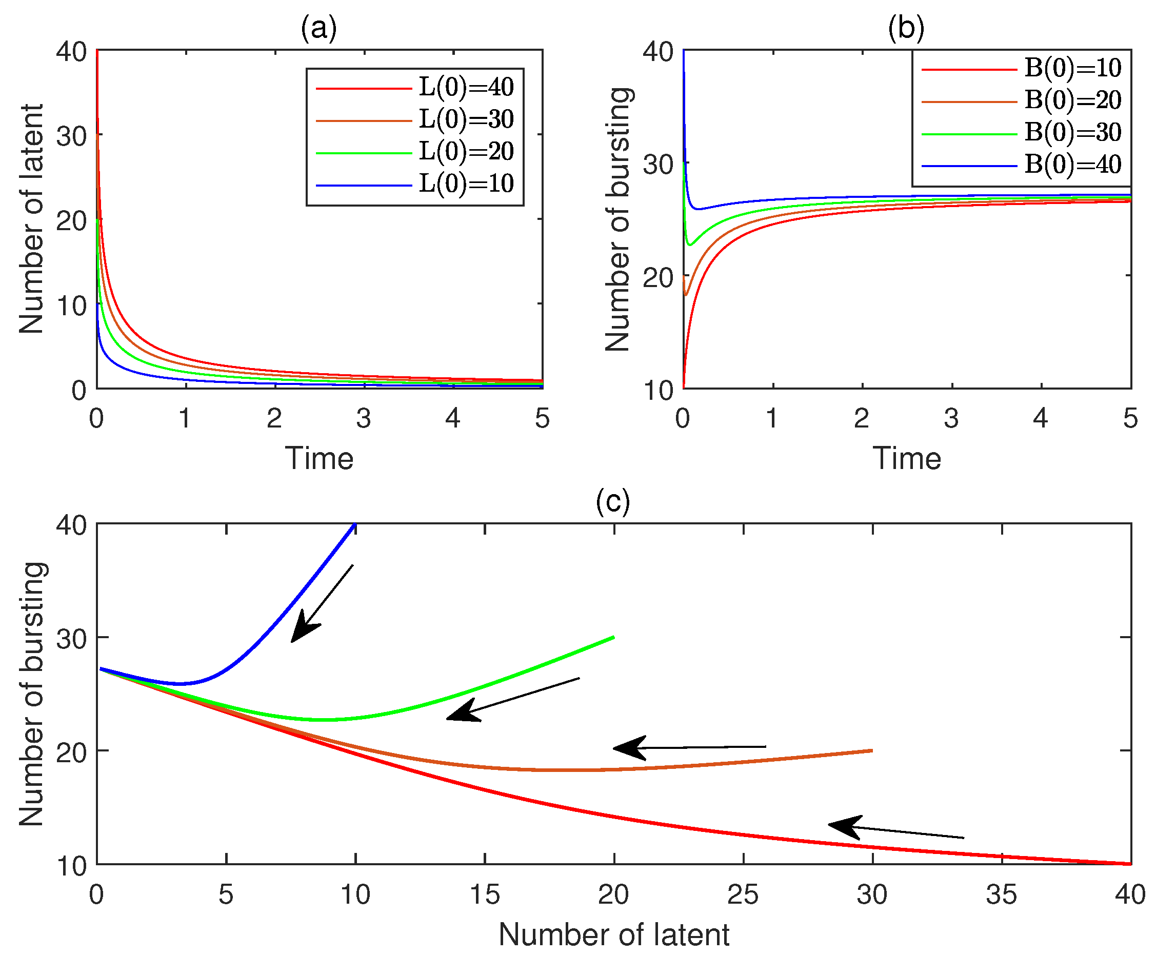
Consider model (23) with α = 0.8 , μ = 40 , δ = 1 , β = 0.15 , η = 1 , γ = 0.5 , and σ = 0.01 . It is easily verified that R 2 > 1 , γ < η , E 1 = ( 0 , 27.27 ) . Hence, it follows from Theorem 6 that E 1 is locally asymptotically stable. For each ( L ( 0 ) , B ( 0 ) ) { ( 40 , 10 ) , ( 30 , 20 ) , ( 20 , 30 ) , ( 10 , 40 ) } , Figure 4a displays the time plot of L ( t ) . Figure 4b displays the time plot of B ( t ) . Figure 4c displays the phase portrait. It is observed that ( L ( t ) , B ( t ) ) E 1 , which is in line with the predicted outcome.
Experiment 5.
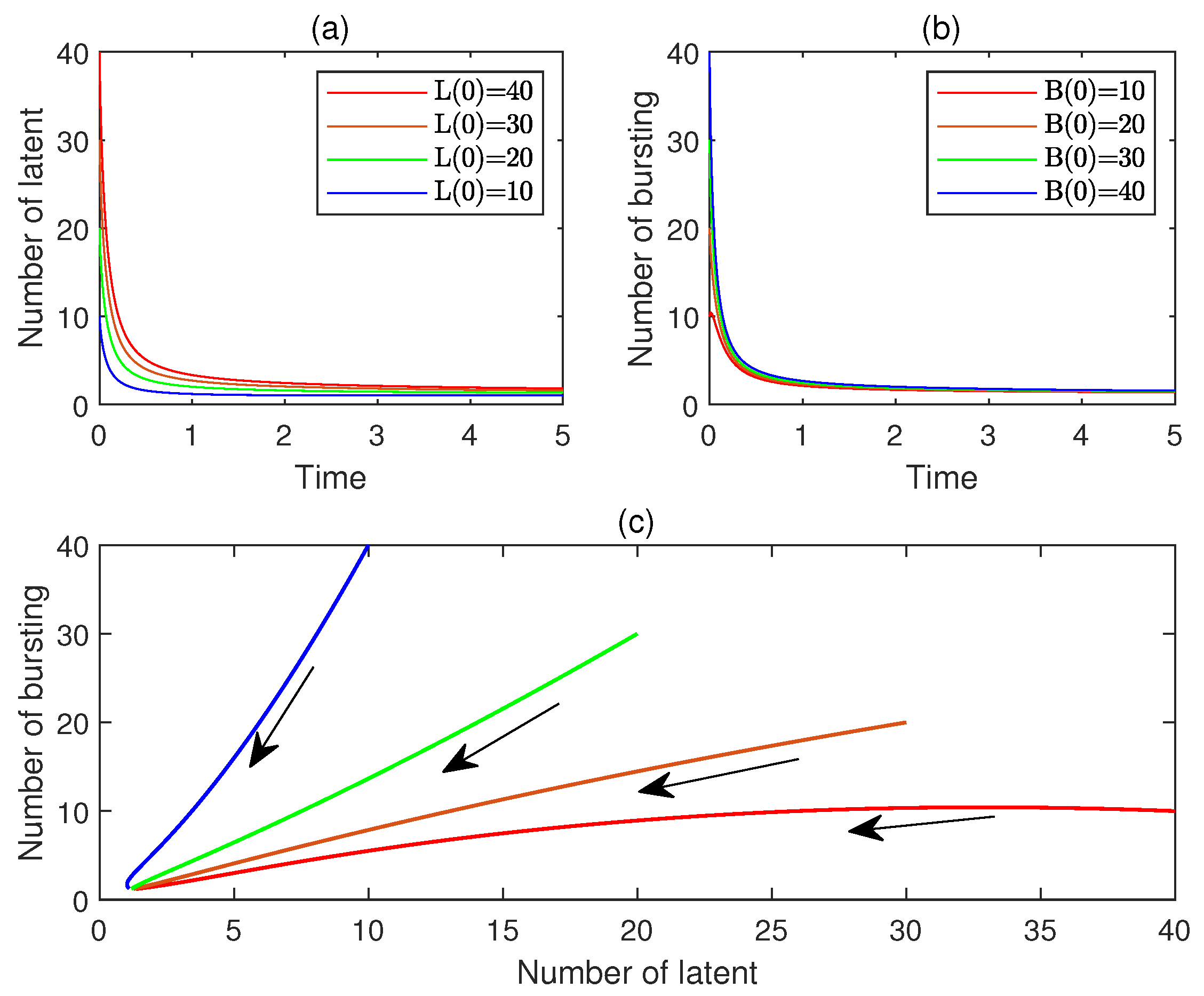
Consider model (23) with α = 0.8 , μ = 40 , δ = 1 , β = 0.15 , η = 1 , γ = 2 , and σ = 0.8 . It is easily verified that R 2 > 1 , γ > η , E 1 = ( 0 , 1.17 ) . It follows from Theorem 6 that E 1 is unstable. For each ( L ( 0 ) , B ( 0 ) ) { ( 40 , 10 ) , ( 30 , 20 ) , ( 20 , 30 ) , ( 10 , 40 ) } , Figure 5a displays the time plot of L ( t ) ; Figure 5b displays the time plot of B ( t ) . Figure 5c displays the phase portrait. It is observed that ( L ( t ) , B ( t ) ) E 1 , which is consistent with the predicted outcome.
Experiment 6.
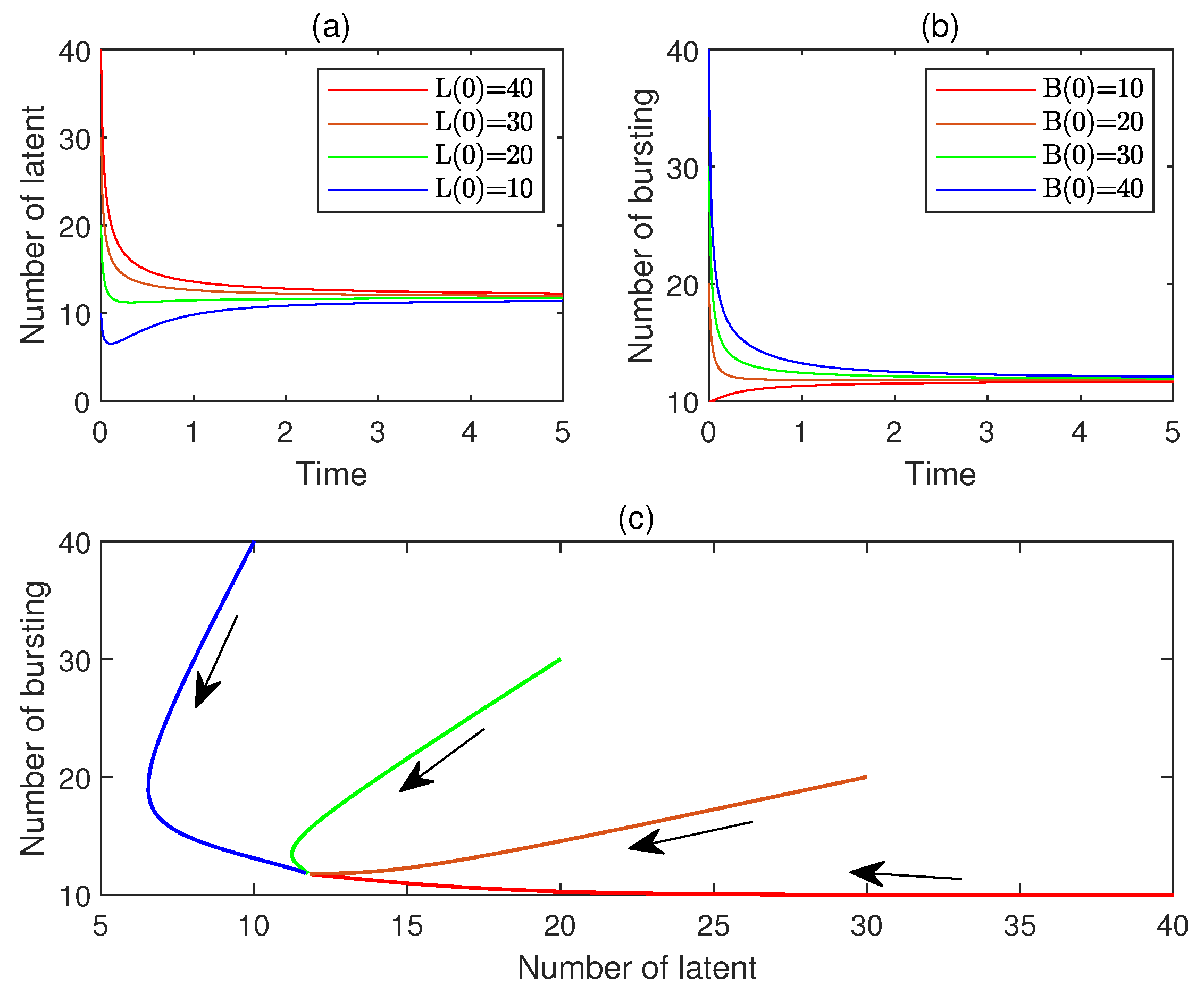
Consider model (23) with α = 0.8 , μ = 40 , δ = 1 , β = 0.15 , η = 1 , γ = 2 , and σ = 0.01 . It easily verified that R 1 > 1 , γ > η , E 2 = ( 11.76 , 11.76 ) , λ 1 = 1.35 , λ 2 = 5.32 , | arg ( λ 1 ) | > α π 2 , | arg ( λ 2 ) | > α π 2 . It follows from Theorem 7 that E 2 is locally asymptotically stable. For each ( L ( 0 ) , B ( 0 ) ) { ( 40 , 10 ) , ( 30 , 20 ) , ( 20 , 30 ) , ( 10 , 40 ) } , Figure 6a displays the time plot of L ( t ) ; Figure 6b displays the time plot of B ( t ) . Figure 6c displays the phase portrait. It is observed that ( L ( t ) , B ( t ) ) E 2 , which is consistent with the predicted outcome.
Experiment 7.
Consider model (23) with α = 0.8 , μ = 80 , δ = 0.15 , β = 0.8 , η = 0.2 , γ = 0.3 , and σ = 1 . It is easily verified that R 1 > 1 , γ > η , E 2 = ( 123.57 , 247.14 ) , λ 1 = 1.91 , λ 2 = 0.48 , | arg ( λ 1 ) | < α π 2 . It follows from Theorem 7 that E 2 is unstable. For each ( L ( 0 ) , B ( 0 ) ) { ( 40 , 10 ) , ( 30 , 20 ) , ( 20 , 30 ) , ( 10 , 40 ) } , Figure 7a displays the time plot of L ( t ) ; Figure 7b displays the time plot of B ( t ) . Figure 7c displays the phase portrait. It is observed that ( L ( t ) , B ( t ) ) E 2 , which is consistent with the predicted outcome.

11. Further Discussions

This section provides further discussions. First, the sensitivity of different model parameters to the basic reproduction number is analyzed. Second, the impact of the fractional order on virus propagation is examined. Next, the impact of the saturation index on virus spread is examined. Finally, the coupling effect of the fractional order and the saturation index on virus propagation is examined.

11.1. Sensitivity Analysis

The following theorem reveals the sensitivity of different model parameters to the basic reproduction number R 0 .
Theorem 8.
The following assertions hold.
(A1) 
S μ = μ R 0 R 0 μ = 1 .
(A2) 
S δ = δ R 0 R 0 δ = min ( η , γ ) + 2 δ min ( η , γ ) + δ .
(A3) 
S β = β R 0 R 0 β = 1 .
(A4) 
S η = η R 0 R 0 η = η η + δ or 0 according as η < γ or η > γ .
(A5) 
S γ = γ R 0 R 0 γ = γ γ + δ or 0 according as γ < η or γ > η .
(A6) 
S σ = σ R 0 R 0 σ = 0 .
Proof of Theorem 8.
R 0 = β μ δ ( η + δ ) if η < γ , β μ δ ( γ + δ ) if η > γ .
The proof of the assertion (A2):
R 0 δ = β μ ( η + 2 δ ) δ 2 ( η + δ ) 2 if η < γ , β μ ( γ + 2 δ ) δ ( γ + δ ) if η > γ .
S δ = δ R 0 R 0 δ = δ β μ δ ( η + δ ) β μ ( η + 2 δ ) δ 2 ( η + δ ) 2 = η + 2 δ η + δ if η < γ , δ β μ δ ( γ + δ ) β μ ( γ + 2 δ ) δ ( γ + δ ) = γ + 2 δ γ + δ if η > γ , = min ( η , γ ) + 2 δ min ( η , γ ) + δ .
The proofs of the remaining assertions are similar. □
The theorem is explained below.
(i)
The entrance rate μ has a significant positive impact on R 0 .
(ii)
The exit rate δ has a significant negative impact on R 0 . Furthermore, the strength of the impact strengthens with the increase in δ .
(iii)
The infection force β has a significant positive impact on R 0 .
(iv)
In the case where η < γ , the burst rate η has a significant negative impact on R 0 . Furthermore, the strength of the impact strengthens with the increase in η .
(v)
In the case where η > γ , the burst rate η has no impact on R 0 .
(vi)
In the case where γ < η , the recovery rate γ has a significant negative impact on R 0 . Furthermore, the strength of the impact strengthens with the increase in γ .
(vii)
In the case where γ > η , the recovery rate γ has no impact on R 0 .
(viii)
The saturation index σ has no impact on R 0 .

11.2. Impact of the Fractional Order

Experiment 8.
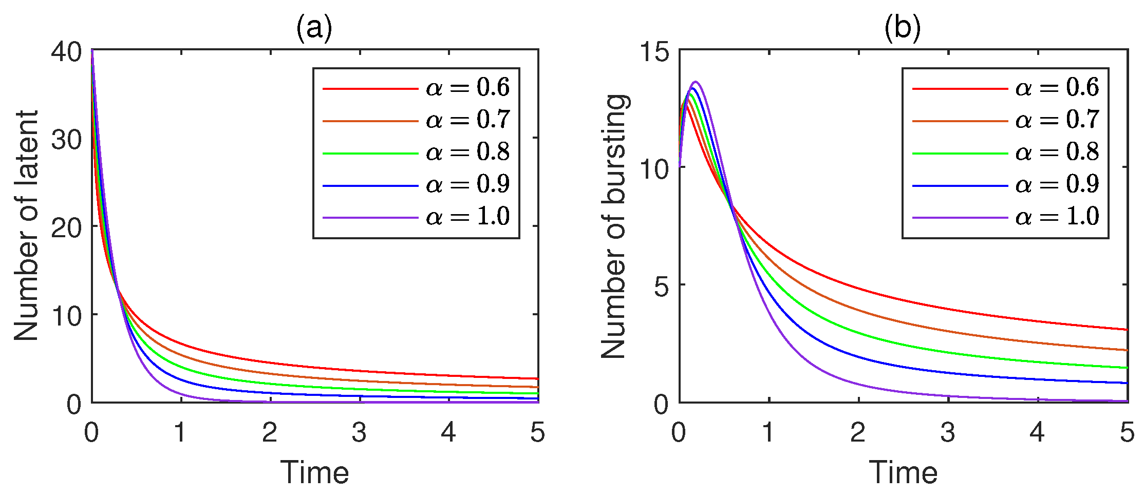
Let α A = { 0.6 , 0.7 . 0.8 , 0.9 , 1.0 } , μ = 80 , δ = 1 , β = 0.015 , η = 1 , γ = 0.5 , σ = 0.6 , and ( L ( 0 ) , B ( 0 ) ) = ( 40 , 10 ) . For each α A , Figure 8a displays the time plot of the corresponding L ( t ) . Figure 8b displays the time plot of the corresponding B ( t ) . It is observed that with the decrease in α, L ( t ) and B ( t ) vary more rapidly at the early stage and vary more slowly at the subsequent stage.
From this experiment, the following conclusions are drawn.
(i)
Compared with the corresponding integer-order model, a fractional-order SLBS model shows a slower spread rate of virus. Furthermore, the smaller the fractional order, the lower the virus propagation rate would be. This reflects the memory effect of the virus and the cumulative impact of historical infection information.
(ii)
The virus does not disappear completely after a long time, maintaining a low-level residual state. This is in line with the actual situation where the latent virus persists in the network.
(iii)
With the change in fractional order, the equilibrium point of virus prevalence can be adjusted flexibly, showing a complex dynamic transition process between different states.

11.3. Impact of the Saturation Index

Experiment 9.
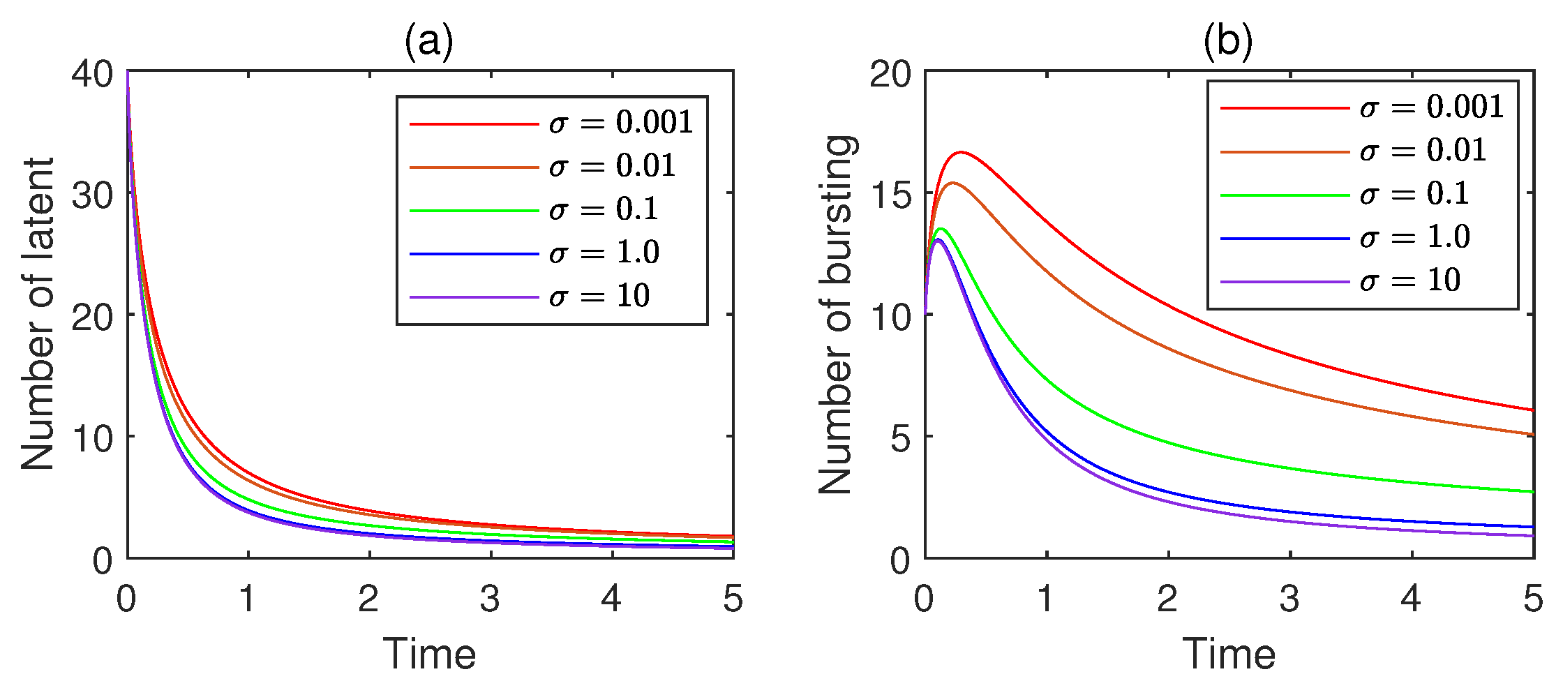
Let α = 0.8 , μ = 80 , δ = 1 , β = 0.015 , η = 1 , γ = 0.5 , σ Σ = { 0.001 , 0.01 , 0.1 , 1.0 , 10 } , and ( L ( 0 ) , B ( 0 ) ) = ( 40 , 10 ) . For each σ Σ , Figure 9a displays the time plot of the corresponding L ( t ) . Figure 9b displays the time plot of the corresponding B ( t ) . It is observed that with the increase in σ, both L ( t ) and B ( t ) tend to lower levels.
Experiment 10.
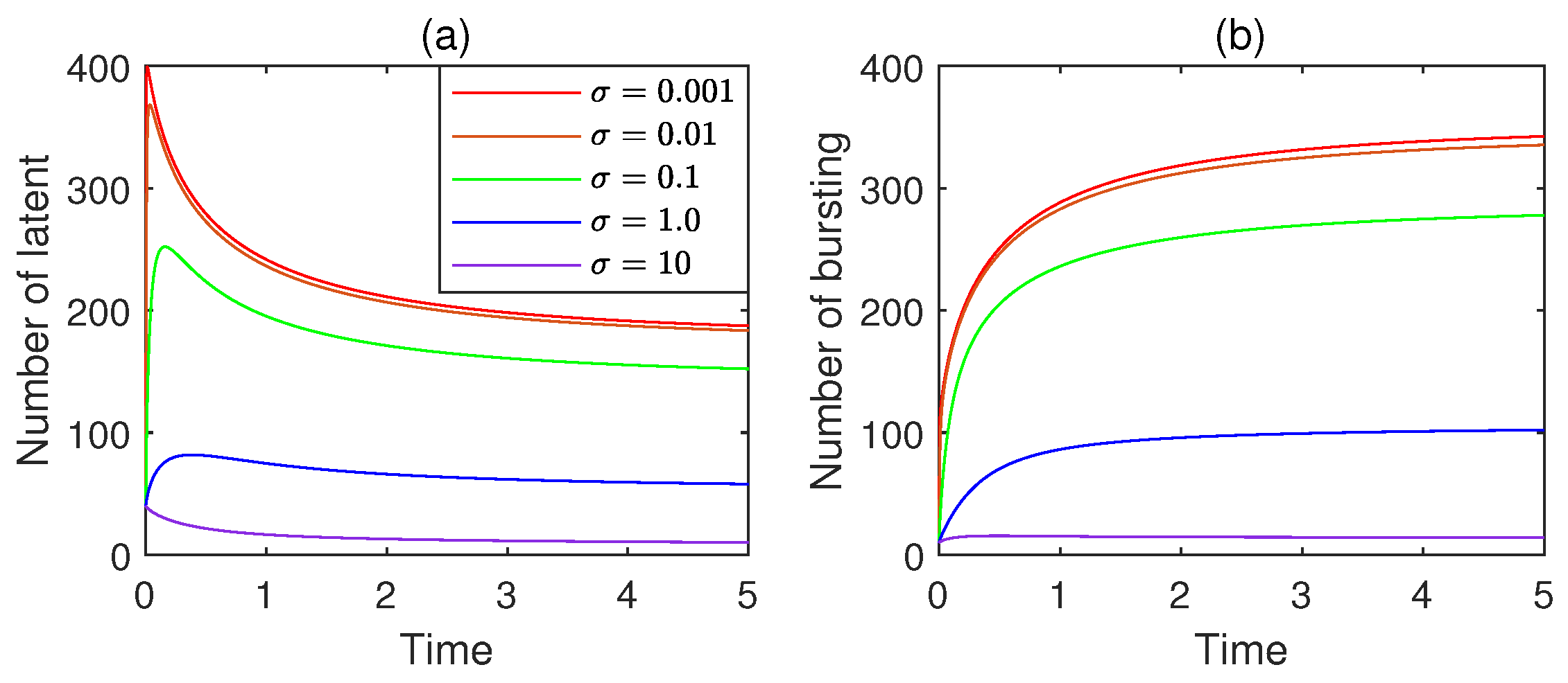
Let α = 0.8 , μ = 40 , δ = 1 , β = 0.15 , η = 1 , γ = 2 , σ Σ = { 0.001 , 0.01 , 0.1 , 1.0 , 10 } , and ( L ( 0 ) , B ( 0 ) ) = ( 10 , 40 ) . For each σ Σ , Figure 10a displays the time plot of the corresponding L ( t ) . Figure 10b displays the time plot of the corresponding B ( t ) . Again, it is observed that with the increase in σ, both L ( t ) and B ( t ) tend to lower levels.
Experiment 11.
Let α = 0.8 , μ = 80 , δ = 0.15 , β = 0.15 , η = 0.2 , γ = 0.3 , σ Σ = { 0.001 , 0.01 , 0.1 , 1.0 , 10 } , and ( L ( 0 ) , B ( 0 ) ) = ( 40 , 10 ) . For each σ Σ , Figure 11a displays the time plot of the corresponding L ( t ) . Figure 11b displays the time plot of the corresponding B ( t ) . Also, it is observed that with the increase in σ, L ( t ) and B ( t ) tend to lower values.
From the above three experiments, the following conclusions are drawn.
(i)
Saturation introduces a natural limit, reflecting real-world constraints like finite vulnerable devices, limited network bandwidth, or activated antivirus measures that slow spread as more devices become infected. Without saturation, the infection rate might grow indefinitely, leading to an implausible scenario where all susceptible devices become infected instantly.
(ii)
The virus spreads rapidly in the early stage when there are many susceptible devices and few barriers. However, as the number of infected devices increases, the infection rate plateaus due to saturation, causing the spread to decelerate. This results in a more realistic sigmoid curve, where the spread eventually stabilizes rather than exploding exponentially.
(iii)
By capturing the diminishing return of virus transmission, where each new infection becomes harder to achieve, this nonlinear saturation aligns the real-world behavior, making predictions of virus prevalence and spread dynamics more reliable.

11.4. Coupling Effect of the Fractional Order and the Saturation Index

Experiment 12.
Let α A = { 0 , 6 , 0.7 , 0.8 , 0.9 , 1.0 } , μ = 80 , δ = 1 , β = 0.015 , η = 1 , γ = 0.5 , σ Σ = { 0.001 , 0.01 , 0.1 , 1.0 , 10 } , and ( L ( 0 ) , B ( 0 ) ) = ( 40 , 10 ) . For each combination ( α , σ ) A × Σ , Figure 12a displays the time plot of the corresponding L ( t ) ; Figure 12b displays the time plot of the corresponding B ( t ) . The following phenomena are observed: (1) With decreases in α, L ( t ) and B ( t ) vary more rapidly at the early stage and vary more slowly at the subsequent stage. (2) With the increase in α and the decrease in σ, L ( t ) and B ( t ) vary violently.
From this experiment, the following conclusions are drawn.
(i)
The coupling with saturation effects manifests as a dynamic interplay where the memory-dependent, non-local propagation characteristics of the fractional-order framework interact with the saturation mechanism, where the propagation rate slows or plateaus as the number of infected nodes approaches a system capacity (e.g., due to limited network resources, enhanced defense responses, or reduced susceptible nodes).
(ii)
The coupling leads to more realistic propagation dynamics, whereby the fractional-order component captures the historical influence and gradual rate changes, while the nonlinear saturation effect constrains excessive spread, reflecting real-world scenarios where propagation is limited by factors like protective measures, network load, or finite susceptible populations. Together, they yield a more accurate depiction of how viruses spread—balancing historical dependencies with the self-limiting nature of large-scale outbreaks.

12. Conclusions

In this article, a fractional computer virus propagation model with saturation effect has been suggested. All possible virus–endemic equilibria of the model have been figured out. Criteria for the local or global asymptotic stability of the virus-free equilibrium are derived. A criterion for the asymptotic stability of each possible virus–endemic equilibrium has been presented. The impact of the fractional order and the saturation index on virus propagation has been reported.
Some relevant issues are yet to be addressed. First, in reality, there exist various time delays in computer virus propagation. For example, there exists a delay from the time an infected computer becomes infected and becomes latent to the time the computer starts bursting, and there also exists a delay from the time a computer starts bursting to the time the computer is repaired. Consequently, it is worthwhile to study fractional computer virus spread models with delays [40,41,42]. Second, the fractional modeling technique of computer virus spread may be used to describe some other types of propagation phenomena, such as virus transmission [43,44,45] and rumor spreading [46,47,48]. Next, fractional virus propagation models may be adapted to the optimal control of malware infections [49,50]. Finally, fractal–fractional differential equations provide a feasible framework for characterizing the dynamical evolution of complex structures with self-similarity, irregularity, and long-term memory nature [51,52]. It is worth investigating fractal–fractional computer virus propagation models [53,54,55].

Author Contributions

Investigation: Z.L. and X.Y.; writing—original draft preparation: X.Y.; writing—review and editing: L.Y. All authors have read and agreed to the published version of the manuscript.

Funding

This research was funded by the Open Fund Project of Intelligent Digital Media Technology Key Laboratory of Sichuan Province, University of Electronic Science and Technology of China (Grant No. ZYGX2025K026-2).

Data Availability Statement

The original contributions presented in this study are included in the article. Further inquiries can be directed to the corresponding author.

Conflicts of Interest

The authors declare no conflicts of interest.

Appendix A. Proof of Lemma 7

Proof of Lemma 7.
Let
x ( t ) = ( S ( t ) , L ( t ) , B ( t ) ) T ,
f 1 ( x ( t ) ) = μ β S ( t ) [ L ( t ) + B ( t ) ] 1 + σ [ L ( t ) + B ( t ) ] + γ B ( t ) δ S ( t ) ,
f 2 ( x ( t ) ) = β S ( t ) L ( t ) 1 + σ [ L ( t ) + B ( t ) ] η L ( t ) δ L ( t ) ,
f 3 ( x ( t ) ) = β S ( t ) B ( t ) 1 + σ [ L ( t ) + B ( t ) ] + η L ( t ) γ B ( t ) δ B ( t ) .
f ( x ( t ) ) = ( f 1 ( x ( t ) , f 2 ( x ( t ) , f 3 ( x ( t ) ) T ,
Then, the model (9) can be abbreviated as follows:
D α x ( t ) = f ( x ( t ) ) , t 0 , x ( 0 ) 0 .
It follows from Lemma 5 that f is continuous.
Let
x 1 = ( S 1 , L 1 , B 1 ) , x 2 = ( S 2 , L 2 , B 2 ) ,
| | f ( x 1 ) f ( x 2 ) | | = | f 1 ( x 1 ) f 1 ( x 2 ) | + | f 2 ( x 1 ) f 2 ( x 2 ) | + | f 3 ( x 1 ) f 3 ( x 2 ) | .
By repeatedly applying the inequality, the following is true:
| a b | = | ( a c ) + ( c b ) | | a c | + | c b | ,
it follows that:
β S 1 ( L 1 + B 1 ) 1 + σ ( L 1 + B 1 ) β S 2 ( L 2 + B 2 ) 1 + σ ( L 2 + B 2 ) β | S 1 ( L 1 + B 1 ) [ 1 + σ ( L 2 + B 2 ) ] S 2 ( L 2 + B 2 ) [ 1 + σ ( L 1 + B 1 ) ] | β ( 1 + 2 σ M ) S 1 ( L 1 + B 1 ) S 2 ( L 2 + B 2 ) + 2 β σ M 2 ( | L 1 L 2 | + | B 1 B 2 | ) β M ( 1 + 2 σ M ) [ 2 | S 1 S 2 | + | L 1 L 2 | + | B 1 B 2 | ] + 2 β σ M 2 ( | L 1 L 2 | + | B 1 B 2 | ) = 2 β M ( 1 + 2 σ M ) | S 1 S 2 | + M ( 1 + 4 σ M ) | L 1 L 2 | + β M ( 1 + 4 σ M ) | B 1 B 2 | ,
β S 1 L 1 1 + σ ( L 1 + B 1 ) β S 2 L 2 1 + σ ( L 2 + B 2 ) β | S 1 L 1 [ 1 + σ ( L 2 + B 2 ) ] S 2 L 2 [ 1 + σ ( L 1 + B 1 ) ] | β ( 1 + 2 σ M ) | S 1 L 1 S 2 L 2 | + β σ M 2 ( | L 1 L 2 | + | B 1 B 2 | ) β M ( 1 + 2 σ M ) [ | L 1 L 2 | + | S 1 S 2 | ] + β σ M 2 ( | L 1 L 2 | + | B 1 B 2 | ) = β M ( 1 + 2 σ M ) | S 1 S 2 | + β M ( 1 + 3 σ M ) | L 1 L 2 | + β σ M 2 | B 1 B 2 | ,
β S 1 B 1 1 + σ ( L 1 + B 1 ) β S 2 B 2 1 + σ ( L 2 + B 2 ) β M ( 1 + 2 σ M ) | S 1 S 2 | + β σ M 2 | L 1 L 2 | + β M ( 1 + 3 σ M ) | B 1 B 2 | .
So,
| f 1 ( x 1 ) f 1 ( x 2 ) | [ 2 β M ( 1 + 2 σ M ) + δ ] | S 1 S 2 | + β M ( 1 + 4 σ M ) | L 1 L 2 | + [ β M ( 1 + 4 σ M ) + γ ] | B 1 B 2 | ,
| f 2 ( x 1 ) f 2 ( x 2 ) | β M ( 1 + 2 σ M ) | S 1 S 2 | + [ β M ( 1 + 3 σ M ) + η + δ ] | L 1 L 2 | + β σ M 2 | B 1 B 2 | ,
| f 3 ( x 1 ) f 3 ( x 2 ) | β M ( 1 + 2 σ M ) | S 1 S 2 | + ( β σ M 2 + η ) | L 1 L 2 | + [ β M ( 1 + 3 σ M ) + γ + δ ] | B 1 B 2 | .
Thus,
| | f ( x 1 ) f ( x 2 ) | | = | f 1 ( x 1 ) f 1 ( x 2 ) | + | f 2 ( x 1 ) f 2 ( x 2 ) | + | f 3 ( x 1 ) f 3 ( x 2 ) | c 1 | S 1 S 2 | + c 2 | L 1 L 2 | + c 3 | B 1 B 2 | ,
where
c 1 = 4 β M ( 1 + 2 σ M ) + δ ,
c 2 = 2 β M ( 1 + 4 σ M ) + 2 η + δ ,
c 3 = 2 β M ( 1 + 4 σ M ) + 2 γ + δ .
Hence, f is globally Lipschitz continuous. It follows from Lemma 1 that model (9) admits a unique solution. □

References

  1. Szor, P. The Art of Computer Virus Research and Defense; Addison-Wesley Professional: Boston, MA, USA, 2005. [Google Scholar]
  2. Blancaflor, E.; Bauson, V.L.; Cruz, A.L.; Escandor, M. Medusa ransomware against data Privacy: A comprehensive study of ransomware attacks across various organizations and strategic recommendations for future prevention. In Proceedings of the 2024 7th International Conference on Information Science and Systems, New York, NY, USA, 31 January 2025; pp. 28–34. [Google Scholar]
  3. Britton, N.F. Essential Mathematical Biology; Springer: Heidelberg/Berlin, Germany, 2003. [Google Scholar]
  4. Kephart, J.O.; White, S.R. Directed epidemiological models of computer viruses. In Proceedings of the 1999 IEEE Computer Society Symposium on Research in Security and Privacy, Los Alamitos, CA, USA, 20–22 May 1991; pp. 343–359. [Google Scholar]
  5. Kephart, J.O.; White, S.R. Measuring and modeling computer virus prevalence. In Proceedings of the 1999 IEEE Computer Society Symposium on Research in Security and Privacy, Los Alamitos, CA, USA, 24–26 May 1993; pp. 2–15. [Google Scholar]
  6. Prakash, O.; Kumar, A.; Bharti, S.K. Computer virus propagation models: A mathematical review. J. Inf. Optim. Sci. 2023, 44, 1043–1055. [Google Scholar] [CrossRef]
  7. Zhang, W.; Yang, X.; Yang, L. A delayed malware propagation model under a distributed patching mechanism: Stability analysis. Mathematics 2025, 13, 2266. [Google Scholar] [CrossRef]
  8. Upadhyay, R.K.; Kumari, S. Bifurcation analysis of an e-epidemic model in wireless sensor network. Int. J. Comput. Math. 2018, 95, 1775–1805. [Google Scholar] [CrossRef]
  9. Yang, F.; Zhang, Z. Dynamics of a nonlinear SIQRS computer virus spreading model with two delays. AIMS Math. 2021, 6, 4083–4104. [Google Scholar] [CrossRef]
  10. Upadhyay, R.K.; Kumari, S.; Misra, A.K. Modeling the virus dynamics in computer network with SVEIR model and nonlinear incident rate. J. Appl. Math. Comput. 2017, 54, 485–509. [Google Scholar] [CrossRef]
  11. Zhao, T.; Zhang, Z.; Upadhyay, R.K. Delay-induced Hopf bifurcation of an SVEIR computer virus model with nonlinear incidence rate. Adv. Differ. Equ. 2018, 2018, 256. [Google Scholar] [CrossRef]
  12. Chu, Y.; Xia, W.; Wang, Z. A delayed computer virus model with nonlinear incidence rate. Syst. Sci. Control Eng. 2019, 7, 389–406. [Google Scholar] [CrossRef]
  13. Yu, X.; Zeb, A.; Zhang, Z. Mathematical analysis of a delayed malware propagation model on mobile wireless sensor network. Fractals 2022, 30, 2240160. [Google Scholar] [CrossRef]
  14. Liu, J.; Saeed, I.; Zeb, A. Delay effect of an e-epidemic SEIRS malware propagation model with a generalized non-monotone incidence rate. Results Phys. 2022, 39, 105672. [Google Scholar] [CrossRef]
  15. Zhang, Z.; Madhusudanan, V.; Murthy, B.S.N. Effect of delay in SMS worm propagation in mobile network with saturated incidence rate. Wirel. Pers. Commun. 2023, 131, 659–678. [Google Scholar] [CrossRef]
  16. Yao, Y.; Fu, Q.; Yang, W.; Wang, Y.; Sheng, C. An epidemic model of computer worms with time delay and variable infection rate. Secur. Commun. Netw. 2018, 2018, 9756982. [Google Scholar] [CrossRef]
  17. Podlubny, I. Fractional Differential Equations; Academic Press: Cambridge, MA, USA, 1999. [Google Scholar]
  18. Zarin, R.; Khaliq, H.; Khan, A.; Khan, D.; Akgul, A.; Humphries, U.W. Deterministic and fractional modeling of a computer virus propagation. Results Phys. 2022, 33, 105130. [Google Scholar] [CrossRef]
  19. Sabir, Z.; Raja, M.A.Z.; Mumtaz, N.; Fathurrochman, I.; Sadat, R.; Ali, M.R. An investigation through stochastic procedures for solving the fractional order computer virus propagation mathematical model with kill signals. Neural Process. Lett. 2023, 55, 1783–1797. [Google Scholar] [CrossRef]
  20. Zhou, Y.; Liu, B.; Zhou, K.; Shen, S. Malware propagation model of fractional order, optimal control strategy and simulations. Front. Phys. 2023, 11, 1201053. [Google Scholar] [CrossRef]
  21. Yang, L.; Song, Q.; Liu, Y. Dynamics analysis of a new fractional-order SVEIR-KS model for computer virus propagation: Stability and Hopf bifurcation. Neurocomputing 2024, 598, 128075. [Google Scholar] [CrossRef]
  22. Shi, X.; Luo, A.; Chen, X.; Huang, Y.; Huang, C.; Yin, X. The dynamical behaviors of a fractional-order malware propagation model in information networks. Mathematics 2024, 12, 3814. [Google Scholar] [CrossRef]
  23. Yang, L.X.; Yang, X.; Zhu, Q.; Wen, L. A computer virus model with graded cure rates. Nonlinear Anal. Real World Appl. 2013, 14, 414–422. [Google Scholar] [CrossRef]
  24. Yang, L.X.; Yang, X. A new epidemic model of computer viruses. Commun. Nonlinear Sci. Numer. Simul. 2014, 19, 1935–1944. [Google Scholar] [CrossRef]
  25. Yang, L.X.; Yang, X. The impact of nonlinear infection rate on the spread of computer virus. Nonlinear Dyn. 2015, 82, 85–95. [Google Scholar] [CrossRef]
  26. Ren, J.; Xu, Y. Stability and bifurcation of a computer virus propagation model with delay and incomplete antivirus ability. Math. Probl. Eng. 2014, 2014, 475934. [Google Scholar] [CrossRef]
  27. Zhao, T.; Wei, S.; Bi, D. Hopf bifurcation of a computer virus propagation model with two delays and infectivity in latent period. Syst. Sci. Control Eng. 2018, 6, 90–101. [Google Scholar] [CrossRef]
  28. Zhang, Z.; Kumari, S.; Upadhyay, R.K. A delayed e-epidemic SLBS model for computer virus. Adv. Differ. Equ. 2019, 2019, 414. [Google Scholar] [CrossRef]
  29. Li, C.; Liao, X. The impact of hybrid quarantine strategies and delay factor on viral prevalence in computer networks. Math. Model. Nat. Phenom. 2016, 11, 105–119. [Google Scholar] [CrossRef]
  30. Zhang, Z.; Upadhyay, R.K.; Bi, D.; Wei, R. Stability and Hopf bifurcation of a delayed epidemic model of computer virus with impact of antivirus software. Discret. Dyn. Nat. Soc. 2018, 2018, 8239823. [Google Scholar] [CrossRef]
  31. Ding, J.; Gul, N.; Liu, G.; Saeed, T. Dynamical aspects of a delayed computer viruses model with horizontal and vertical dissemination over internet. Fractals 2023, 31, 2340092. [Google Scholar] [CrossRef]
  32. Angstmann, C.N.; Henry, B.I.; McGann, A.V. A fractional-order infectivity SIR model. Phys. A 2016, 452, 8239823. [Google Scholar] [CrossRef]
  33. Angstmann, C.N.; Erickson, A.M.; Henry, B.I.; McGann, A.V.; Murray, J.M.; Nichols, J.A. A general framework for fractional order compartment models. SIAM Rev. 2021, 63, 375–392. [Google Scholar] [CrossRef]
  34. Xiao, D.; Ruan, S. Global analysis of an epidemic model with nonmonotone incidence rate. Math. Biosci. 2007, 208, 86–93. [Google Scholar] [CrossRef]
  35. Buonomo, B.; Rionero, S. On the Lyapunov stability for SIRS epidemic models with general nonlinear incidence rate. Appl. Math. Comput. 2010, 217, 4010–4016. [Google Scholar] [CrossRef]
  36. Diekmann, O.; Heesterbeek, J.A.P.; Metz, J.A.J. On the definition and the computation of the basic reproduction ratio R0 in models for infectious diseases in heterogeneous populations. J. Math. Biol. 1990, 28, 365–382. [Google Scholar] [CrossRef]
  37. van den Driessche, P.; Watmough, J. Reproduction numbers and sub-threshold endemic equilibria for compartmental models of disease transmission. Math. Biosci. 2002, 180, 29–48. [Google Scholar] [CrossRef] [PubMed]
  38. Robinson, R. An Introduction to Dynamical Systems: Continuous and Discrete; Pearson Education, Inc.: London, UK, 2005. [Google Scholar]
  39. Diethelm, K.; Neville, J.; Ford, N.J.; Freed, A.D. A predictor-correction approach approach for the numerical solution of fractional differential equations. Nonlinear Dyn. 2002, 29, 3–22. [Google Scholar] [CrossRef]
  40. Wu, G.; Zhang, Y.; Zhang, H.; Yu, S.; Yu, S.; Shen, S. SIHQR model with time delay for worm spread analysis in IIoT-enabled PLC network. Ad Hoc Netw. 2024, 160, 103504. [Google Scholar] [CrossRef]
  41. Nithya, D.; Madhusudanan, V.; Murthy, B.S.N.; Geetha, R.; Mung, N.X.; Dao, N.; Cho, S. Delayed dynamics analysis of SEI2RS malware propagation models in cyber–Physical systems. Comput. Netw. 2024, 248, 110481. [Google Scholar] [CrossRef]
  42. Wang, J.; Chang, X. A SEIQRS computer virus propagation model and impulse control with two delays. Math. Methods Appl. Sci. 2025, 48, 6851–6865. [Google Scholar] [CrossRef]
  43. Hanif, A.; Butt, A.I.K.; Ahmad, W. Numerical approach to solve Caputo-Fabrizio-fractional model of corona pandemic with optimal control design and analysis. Math. Methods Appl. Sci. 2023, 46, 9751–9782. [Google Scholar] [CrossRef]
  44. Butt, A.I.K.; Imran, M.; Azeem, K.; Ismaeel, T.; McKinney, B.A. Analyzing HIV/AIDS dynamics with a novel Caputo-Fabrizio fractional order model and optimal control measures. PLoS ONE 2024, 19, e0315850. [Google Scholar] [CrossRef]
  45. Imran, M.; Butt, A.I.K.; McKinney, B.A.; Al Nuwairan, M.; Al Mukahal, F.H.H.; Batool, S. A comparative analysis of different fractional optimal control strategies to eradicate Bayoud disease in date palm trees. Fractal Fract. 2025, 9, 260. [Google Scholar] [CrossRef]
  46. Ye, M.; Jiang, H. Bifurcation control for a fractional-order delayed SEIR rumor spreading model with incommensurate orders. Acta Math. Sci. 2023, 43B, 2662–2682. [Google Scholar] [CrossRef]
  47. Wei, C.; Fu, C.; Yang, X.; Qin, Y.; Yang, L. Stability analysis of a rumor-spreading model with two time delays and saturation effect. Mathematics 2025, 13, 1729. [Google Scholar] [CrossRef]
  48. Sheng, T.; Fu, C.; Yang, X.; Qin, Y.; Yang, L. Asymptotic stability of a rumor spreading model with three time delays and two saturation functions. Mathematics 2025, 13, 2015. [Google Scholar] [CrossRef]
  49. Jafar, M.T.; Yang, L.X.; Li, G.; Zhu, Q.; Gan, C. Minimizing malware propagation in Internet of Things networks: An optimal control using feedback loop approach. IEEE Trans. Inf. Forensics Secur. 2024, 19, 9682–9697. [Google Scholar] [CrossRef]
  50. Liu, G.; Fu, C.; Yang, X.; Yang, L.; Feng, Y.; Qin, Y. Study of the antivirus patch testing problem through optimal control modeling. PLoS ONE 2025, 20, e0319916. [Google Scholar] [CrossRef] [PubMed]
  51. Atangana, A. Fractal-fractional differentiation and integration: Connecting fractal calculus and fractional calculus to predict complex system. Chaos Solitons Fractals 2017, 102, 396–406. [Google Scholar] [CrossRef]
  52. Atangana, A.; Akgul, A.; Owolabi, K.M. Analysis of fractal fractional differential equations. Alex. Eng. J. 2020, 59, 1117–1134. [Google Scholar] [CrossRef]
  53. Akgul, A.; Fatima, U.; Iqbal, M.S.; Ahmed, N.; Raza, A.; Iqbal, Z.; Rafiq, M. A fractal fractional model for computer virus dynamics. Chaos Solitons Fractals 2021, 147, 110947. [Google Scholar] [CrossRef]
  54. Razi, N.; Bano, A.; Ishtiaq, U.; Kamran, T.; Garayev, M.; Popa, I.-L. Probing malware propagation model with variable infection rates under integer, fractional, and fractal–fractional orders. Fractal Fract. 2025, 9, 90. [Google Scholar] [CrossRef]
  55. Althubyani, M.; Saber, S. Hyers–Ulam stability of fractal–fractional computer virus models with the Atangana–Baleanu Operator. Fractal Fract. 2025, 9, 158. [Google Scholar] [CrossRef]
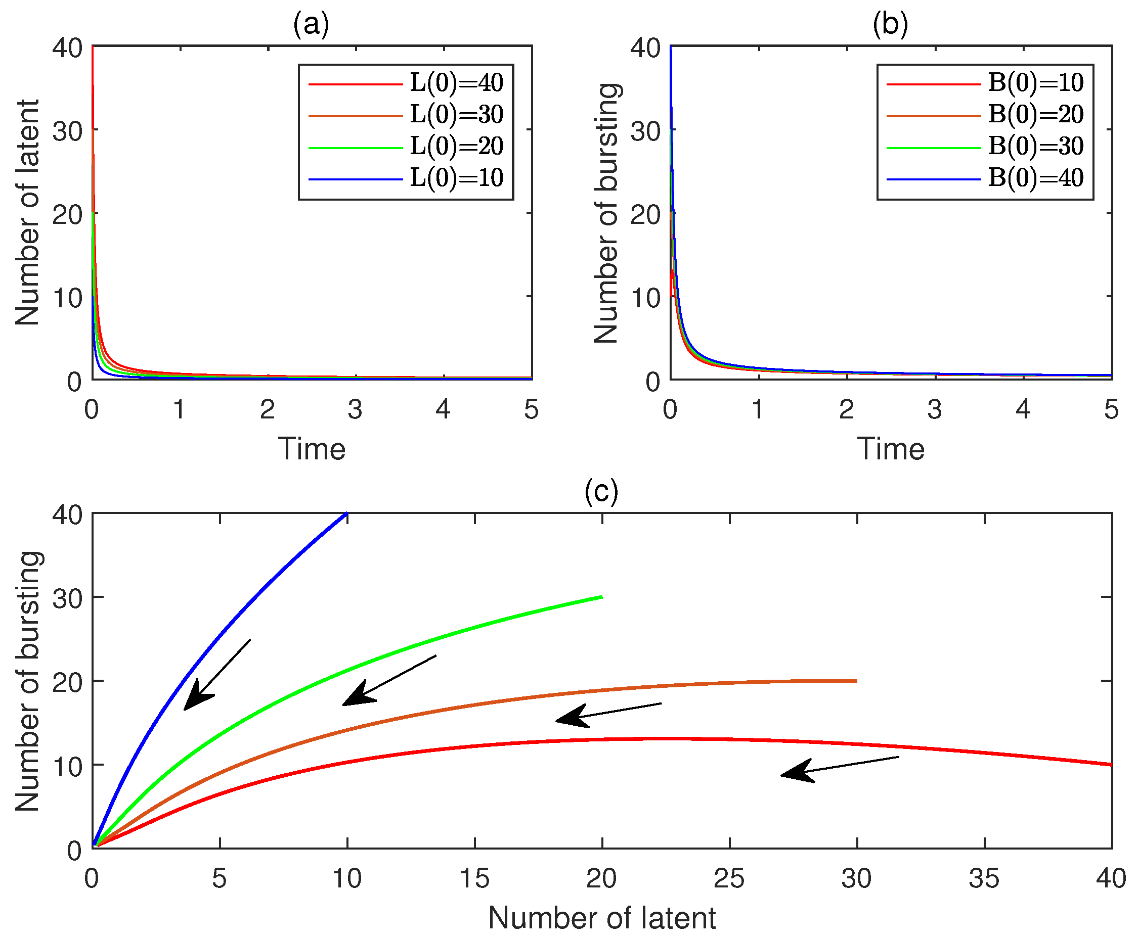
Figure 1. Experimental results of Experiment 1: (a) the time plot of L ( t ) , (b) the time plot of B ( t ) , (c) the phase portrait.
Fractalfract 09 00587 g001
Figure 2. Experimental results of Experiment 2: (a) the time plot of L ( t ) , (b) the time plot of B ( t ) , (c) the phase portrait.
Fractalfract 09 00587 g002
Figure 3. Experimental results of Experiment 3: (a) the time plot of L ( t ) , (b) the time plot of B ( t ) , (c) the phase portrait.
Fractalfract 09 00587 g003
Figure 4. Experimental results of Experiment 4: (a) the time plot of L ( t ) , (b) the time plot of B ( t ) , (c) the phase portrait.
Fractalfract 09 00587 g004
Figure 5. Experimental results of Experiment 5: (a) the time plot of L ( t ) , (b) the time plot of B ( t ) , (c) the phase portrait.
Fractalfract 09 00587 g005
Figure 6. Experimental results of Experiment 6: (a) the time plot of L ( t ) , (b) the time plot of B ( t ) , (c) the phase portrait.
Fractalfract 09 00587 g006
Figure 7. Experimental results of Experiment 7: (a) the time plot of L ( t ) , (b) the time plot of B ( t ) , (c) the phase portrait.
Fractalfract 09 00587 g007
Figure 8. Result of Experiment 8: (a) the time plot of L ( t ) , (b) the time plot of B ( t ) .
Fractalfract 09 00587 g008
Figure 9. Result of Experiment 9: (a) the time plot of L ( t ) , (b) the time plot of B ( t ) .
Fractalfract 09 00587 g009
Figure 10. Result of Experiment 10: (a) the time plot of L ( t ) , (b) the time plot of B ( t ) .
Fractalfract 09 00587 g010
Figure 11. Result of Experiment 11: (a) the time plot of L ( t ) , (b) the time plot of B ( t ) .
Fractalfract 09 00587 g011
Figure 12. Result of Experiment 10: (a,b) the time plot of L ( t ) , (c,d) the time plot of B ( t ) .
Fractalfract 09 00587 g012
Disclaimer/Publisher’s Note: The statements, opinions and data contained in all publications are solely those of the individual author(s) and contributor(s) and not of MDPI and/or the editor(s). MDPI and/or the editor(s) disclaim responsibility for any injury to people or property resulting from any ideas, methods, instructions or products referred to in the content.