Numerical Investigation for the Temporal Fractional Financial Option Pricing Partial Differential Equation Utilizing a Multiquadric Function

Abstract

This paper proposes a computational procedure to resolve the temporal fractional financial option pricing partial differential equation (PDE) using a localized meshless approach via the multiquadric radial basis function (RBF). Given that financial market information is best characterized within a martingale framework, the resulting option pricing model follows a modified Black–Sholes (BS) equation, requiring efficient numerical techniques for practical implementation. The key innovation in this study is the derivation of analytical weights for approximating first and second derivatives, ensuring improved numerical stability and accuracy. The construction of these weights is grounded in the second integration of a variant of the multiquadric RBF, which enhances smoothness and convergence properties. The performance of the presented solver is analyzed through computational tests, where the analytical weights exhibit superior accuracy and stability in comparison to conventional numerical weights. The results confirm that the new approach reduces absolute errors, demonstrating its effectiveness for financial option pricing problems.

1. Background and Preliminaries

The Black–Sholes (BS) partial differential equation (PDE) serves as a foundational model in option pricing theory. However, various enhancements have been proposed to address its limitations [1] (Chapter 7), [2]. The growing utilization of fractional differential equations (FDEs) in financial modeling has led to new developments in option pricing [3,4]. In particular, Wyss [5] studied a time-fraction BS problem to price European vanilla options, leveraging the fractional Brownian motion (FBM) framework. This model introduces a Hurst exponent taking real values, $0<H<1$, that captures the memory effects in financial time series [6]. Unlike traditional Itô stochastic differential equations (SDEs) [7], fractional SDEs pose additional analytical challenges but offer an improved representation of stock market volatility, where price variations can be better described using a time differential of order ${\left(dt\right)}^H$. Despite these advantages, dealing with FBM-based models in option pricing remains nontrivial, as certain financial assets exhibit long-memory characteristics, wherein correlations between returns diminish at a slow rate.

Let $\mu$, r, and $\sigma$ denote the expected return, risk-free rate of interest, and volatility, respectively. Also, let the price dynamics of $S_t$ follow a fractional SDE (FSDE) of the form (refer to, for instance, [5,8]):

$$d{S}_t=(r-q)S_{t}dt+\sigma S_t{W}_t{\left(dt\right)}^H,$$

(1)

or alternatively, as shown in [9]:

$$d^{\alpha }{S}_t=(\mu -q)S_t{\left(dt\right)}^{\alpha }+\sigma S_{t}d{W}_t,$$

(2)

where q represents the return from dividends, $W_t$ is a standard normal white noise process, and $\alpha =2H$. Here, the fractional derivative in (1) reflects the long-memory effect in asset price evolution.

Moreover, empirical evidence suggests that stock returns tend to exhibit clustering behavior, a feature that is absent in classical semi-martingale models such as the standard BS equation. This observation has motivated researchers to explore fractional-order models, which often provide a more accurate representation of market dynamics [10]. From a modeling perspective, one major challenge is that FBM is not a semi-martingale, preventing direct application of Itô calculus. One possible approach involves replacing the Itô integral with a modified Riemann-Stieltjes integral. However, as demonstrated in [11], such a formulation allows arbitrage opportunities, contradicting real-world market behavior. To address this, Hu [12] introduced a new stochastic integral using the Wick product and integral of the Skorokhod, proving that the resulting model is arbitrage-free. Nonetheless, Björk and Hult [13] later argued that this model lacks clear economic interpretation. Guasoni [14] showed that introducing proportional transaction costs into the fractional BS PDE eliminates arbitrage opportunities, aligning it more closely with empirical observations [15]. Additionally, Norros et al. [16] proposed a fundamental martingale that shares the same filter as FBM while retaining financial interpretability.

Let $b(S_t,t)$ denote the value of a contingent claim with final payoff $b(S_T,T)$ at maturity $T>0$. Assuming a deterministic interest rate r and employing a fundamental martingale to ensure an arbitrage-free pricing framework, one obtains the following time-fractional PDE [8]:

$${\displaystyle \frac{{\partial }^{\alpha }b(s,\tau )}{\partial {\tau }^{\alpha }}}={\displaystyle \frac{1}{2}}{\sigma }^2{s}^2{\displaystyle \frac{{\partial }^{2}b(s,\tau )}{\partial s^2}}+(r-q)s{\displaystyle \frac{\partial b(s,\tau )}{\partial s}}-rb(s,\tau ),s\ge 0,$$

(3)

where $\tau =T-t$ denotes time until expiration, and the time differentiation is defined in terms of the right-sided modified Riemann–Liouville (RL) differentiation for $0<\alpha \le 1$. When $\alpha =1$ (equivalently, $H=1/2$), Equation (3) simplifies to the classic BS PDE. The scalars $\sigma$ and q represent a suitable parameter, and dividend yield, respectively.

The existence and uniqueness of resolutions to time-fractional PDEs have been extensively investigated. Luchko [17] established the uniqueness of classical resolutions utilizing the maximum principle, while Batogna and Atangana [18] provided further theoretical insights. Specifically, for a bounded function b, there exists a constant $\varsigma >0$ such that for appropriate positive scalars $t_1$ and $t_2$:

$$\parallel \beta \left(b(s,t_2)\right)-\beta \left(b(s,t_1)\right)\parallel \le \varsigma \parallel b(s,t_2)-b(s,t_1)\parallel ,$$

where $\beta :\mathcal{H}\to \mathcal{H}$ is a contraction mapping defined on a Sobolev space $\mathcal{H}$.

Remark 1. 

Alternative PDE formulations incorporating the Hurst index have been proposed, differing primarily in coefficient structure [8,19]. In this study, we focus on Equation (3), but our numerical methodology can be readily adapted to other fractional PDEs.

The incorporation of fractional derivatives in (3) introduces long-memory effects in asset returns. Lo [20] highlighted the significance of long-memory components in financial models, emphasizing their impact on modern financial theory.

The modified RL fractional derivative, as introduced in [21] (p. 1369), is defined for a continuous function v as:

$$v^{\left(\alpha \right)}\left(\tau \right):={\displaystyle \frac{d^{\alpha }v\left(\tau \right)}{d{\tau }^{\alpha }}}=\left\{\begin{array}{cc}{\displaystyle {\displaystyle \frac{1}{\Gamma (-\alpha )}}{\int }_0^{\tau }{(\tau -\psi )}^{-\alpha -1}(v\left(\tau \right)-v\left(0\right))d\psi ,}\hfill & \alpha <0,\hfill \\ {\displaystyle {\displaystyle \frac{1}{\Gamma (1-\alpha )}}{\displaystyle \frac{d}{d\tau }}{\int }_0^{\tau }{(\tau -\psi )}^{-\alpha }(v\left(\psi \right)-v\left(0\right))d\psi ,}\hfill & 0<\alpha <1,\hfill \\ {\displaystyle {\displaystyle \frac{d^{\theta }\left(v^{(\alpha -\theta )}\left(\tau \right)\right)}{d{\tau }^{\theta }}},}\hfill & \theta \le \alpha <\theta +1,\theta \ge 1.\hfill \end{array}\right.$$

(4)

where $\Gamma (·)$ is the function of Gamma, and $\theta$ is a suitable scalar. The scenario $0<\alpha <1$ is relevant to the fractional PDE in (3).

Since the filter process, rather than the stochastic process itself, characterizes market information, employing a martingale framework in option pricing is a rational choice. This leads to a formulation of the BS equation analogous to its classical counterpart but requiring numerical methods for practical implementation.

The contribution of this manuscript lies in proposing a new numerical method via the local meshless methods for solving (3) efficiently. Toward this target, the main novelty lies in

• obtaining analytical weights for approximating the initial and secondary derivatives of a given function,
• and then employing them in solving the practical financial PDE problem.

The organization of this manuscript is furnished as follows. Section 2 gives the details of the meshless schemes and their implementation in solving PDE problems. Next, in Section 3 first the integrations of a variant of multiquadric (MQ) radial basis function (RBF) are computed. We build our new set of weights based on the second integration of this function. The motivation of such a choice is not only to bring novelty and extend the discussions in [22,23] but also to give further smoothness of the RBF by working on its second-order integration. New weights for approximating the derivatives are constructed therein, and the convergence order of the approximations is presented. 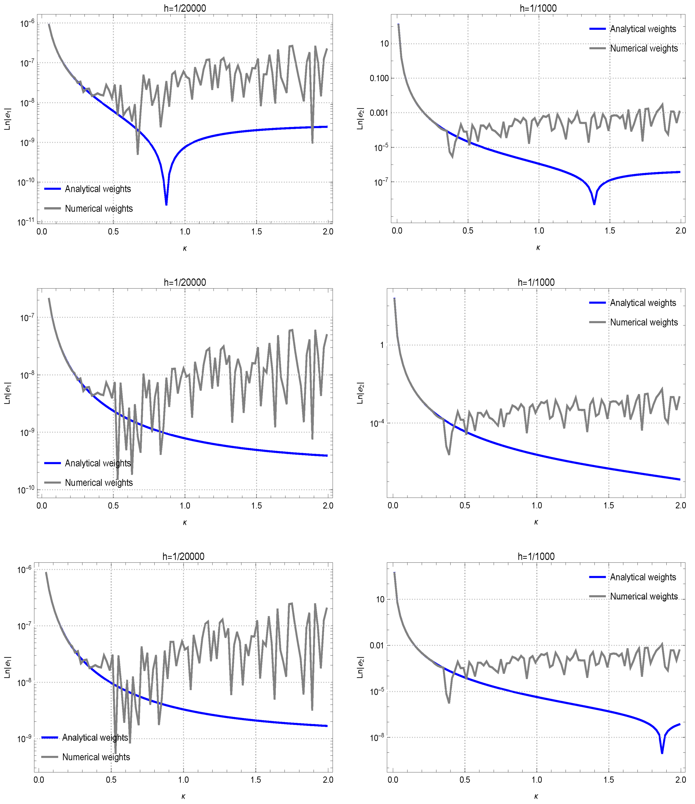Then, Section 4 presents the comparisons between the analytical and numerical weights to clearly highlight the importance and advantages of the new weights in practice when then overcome the stability issues and provide robustness. Section 5 furnishes the procedure of solving (3) using the new weights. The computational pieces of evidence are provided in Section 6, highlighting the usefulness and applicability of the new weights in resolving a practical problem in finance. Concluding remarks and future directions are furnished in the Section 7.

2. The Methodology of Localized Meshless Methods

The RBF-generated finite difference (FD) framework is an advanced numerical method that extends classical FD methods to unstructured point distributions [24,25]. Unlike conventional FD approaches, which depend on regular grid structures, RBF-FD leverages scattered knots to estimate function differentiations. This characteristic renders it adaptable for solving difficult PDEs. Such flexibility proves particularly advantageous in finance.

In the RBF-FD technique, differentiation matrices (DMs) are constructed utilizing RBFs. Given a set of N scattered distinct knots $\left\{y_i\right\}$ within the computational domain, $k\left(y\right)$ is represented as a linear superposition of RBFs [26]:

$$k\left(y\right)\approx \sum _{i=1}^m{\lambda }_i\varphi (\parallel y-y_i\parallel ),$$

(5)

where $\varphi (·)$ denotes a RBF, and ${\lambda }_i$ are the unknowns. The stencil utilized in this formulation consists of the central node $y_c$ and its $m-1$ nearest neighboring points, where $m\ll N$.

To obtain derivative approximations, the differentiation matrix (DM) is derived by computing a localized set of equations inside a stencil consisting of the m closest points. This localized formulation guarantees the sparsity of the matrix of the system, thereby improving computational efficacy. For every $i\in \{1,2,\dots ,m\}$, the derivative based on the stencil is expressed as:

$${\displaystyle \frac{\partial k}{\partial y}}{|}_{y_i}\approx \sum _{j=1}^m{w}_{j}k\left(y_j\right),$$

(6)

wherein $w_j$ are coefficients obtained through the process for RBF interpolation (5). For the derivatives of second order, an analogous formula is employed utilizing 2nd-order DMs. A fundamental merit of RBF-FD over traditional FD solvers lies in its capacity to accommodate non-uniform nodes [27]. The accuracy and stability of the scheme are influenced by key factors, including the choice of RBF, stencil size, and shape parameter choice.

3. Construction of the Novel Weighting Coefficients

Here, we provide a modified form of the infinitely smooth MQ RBF [26], which is defined as:

$$f\left(\chi \right)={({\kappa }^2+{\chi }^2)}^{-3/2},$$

(7)

where $\kappa$ represents the shape parameter governing the smoothness of the function, while $\chi$ corresponds to the radial distance. The exponent $-3/2$ has been chosen to enhance the flexibility and adaptability of the MQ function. Importantly, this particular formulation—previously unexplored in the literature—yields a novel set of weights designed to calculate the first and second derivatives of a suitable function, see also [28].

To gain deeper insights into this formulation, we examine the functions obtained via integrating the expression (7). The first and second integrals of (7) in a one-dimensional setting are obtained in terms of Euclidean distance and are given by:

$$\begin{array}{cc}\hfill & f^1\left(\chi \right)={\displaystyle \frac{\chi \left(\frac{{\chi }^2}{{\kappa }^2}+1\right)}{{\left({\kappa }^2+{\chi }^2\right)}^{3/2}}},\hfill \end{array}$$

(8)

$$\begin{array}{cc}\hfill & f^2\left(\chi \right)={\displaystyle \frac{{\left(\frac{{\chi }^2}{{\kappa }^2}+1\right)}^{3/2}\left({\kappa }^2\left(\frac{1}{{\left(\frac{{\chi }^2}{{\kappa }^2}+1\right)}^{3/2}}-1\right)+\frac{{\chi }^2}{{\left(\frac{{\chi }^2}{{\kappa }^2}+1\right)}^{3/2}}+\frac{{\chi }^2}{\sqrt{\frac{{\kappa }^2+{\chi }^2}{{\kappa }^2}}}\right)}{{\left({\kappa }^2+{\chi }^2\right)}^{3/2}}}.\hfill \end{array}$$

(9)

Based on these integral formulations, we move forward with determining the corresponding coefficients within the RBF-FD methodology in one dimension. The derivation focuses on the second integral of the MQ function (7) and its relationship with (9).

Again assume a set of discrete nodes, $Y=\{y_1,y_2,\dots ,y_N\}$, which constitutes a partition of the computational domain. Building upon this discretization, we present a 3-node unequally-spaced configuration defined as:

$$\{y_{i-1},y_i,y_{i+1}\}=\{y_i-h,y_i,y_i+ph\},h>0,$$

(10)

Here, p controls the spacing among the three closest neighboring knots, whose positions adhere to $y_{i+1}=y_i+ph$. The parameter p plays a crucial role in controlling the separation between the central point and its forward neighbor in a one-dimensional framework. Notably, when applied to a non-uniform discretization, this value dynamically varies for every set of three adjacent nodes.

For the particular case where $m=3$, the formulation given in (6) is employed, as previously presented in [29,30]:

$$\begin{array}{cc}\hfill k^{\prime }\left(y_i\right)\simeq & {\widehat{k}}^{\prime }\left(y_i\right)={\varrho }_{i-1}k\left(y_{i-1}\right)+{\varrho }_{i}k\left(y_i\right)+{\varrho }_{i+1}k\left(y_{i+1}\right),2\le i\le N-1,\hfill \end{array}$$

(11)

where ${\widehat{k}}^{\prime }$ represents an approximate of the first derivative. To move forward, the relation (9) is utilized, resulting in

$$\begin{array}{cc}\hfill & -\kappa \left({\displaystyle \frac{{\left(\frac{h^2}{{\kappa }^2}+1\right)}^{3/2}\left(\frac{h^2{\varrho }_i}{{\left(\frac{h^2}{{\kappa }^2}+1\right)}^{3/2}}+\frac{h\left(h{\varrho }_i-1\right)}{\sqrt{\frac{h^2}{{\kappa }^2}+1}}+\frac{{\kappa }^2{\varrho }_i}{{\left(\frac{h^2}{{\kappa }^2}+1\right)}^{3/2}}-{\kappa }^2{\varrho }_i\right)}{{\left(h^2+{\kappa }^2\right)}^{3/2}}}+{\displaystyle \frac{{\varsigma }_1}{{\left({(hp+h)}^2+{\kappa }^2\right)}^{3/2}}}\right)=0,\hfill \end{array}$$

(12)

$$\begin{array}{cc}\hfill & -{\displaystyle \frac{\left(\frac{h^2}{\sqrt{\frac{h^2}{{\kappa }^2}+1}}+\frac{h^2+{\kappa }^2}{{\left(\frac{h^2}{{\kappa }^2}+1\right)}^{3/2}}-{\kappa }^2\right){\left(\frac{h^2}{{\kappa }^2}+1\right)}^{3/2}{\varrho }_{i-1}}{{\left(h^2+{\kappa }^2\right)}^{3/2}}}-{\displaystyle \frac{{\varsigma }_2}{{\left(h^2{p}^2+{\kappa }^2\right)}^{3/2}}}=0,\hfill \end{array}$$

(13)

$$\begin{array}{cc}\hfill & {\varsigma }_3-{\displaystyle \frac{{\varrho }_{i-1}\left(\frac{h^2{(p+1)}^2}{\sqrt{\frac{{(hp+h)}^2}{{\kappa }^2}+1}}+{\kappa }^2\left(\frac{1}{\sqrt{\frac{h^2{(p+1)}^2}{{\kappa }^2}+1}}-1\right)\right){\left(\frac{h^2{(p+1)}^2}{{\kappa }^2}+1\right)}^{3/2}}{{\left(h^2{(p+1)}^2+{\kappa }^2\right)}^{3/2}}}=0,\hfill \end{array}$$

(14)

where

$$\begin{array}{cc}\hfill & {\varsigma }_1={\varrho }_{i+1}\left({\displaystyle \frac{h^2{(p+1)}^2}{\sqrt{\frac{{(hp+h)}^2}{{\kappa }^2}+1}}}+{\kappa }^2\left({\displaystyle \frac{1}{\sqrt{\frac{h^2{(p+1)}^2}{{\kappa }^2}+1}}}-1\right)\right){\left({\displaystyle \frac{{(hp+h)}^2}{{\kappa }^2}}+1\right)}^{3/2},\hfill \\ \hfill & {\varsigma }_2={\varrho }_{i+1}{\left({\displaystyle \frac{h^2{p}^2}{{\kappa }^2}}+1\right)}^{3/2}\left({\displaystyle \frac{h^2{p}^2}{\sqrt{\frac{h^2{p}^2}{{\kappa }^2}+1}}}+{\displaystyle \frac{h^2{p}^2+{\kappa }^2}{{\left(\frac{h^2{p}^2}{{\kappa }^2}+1\right)}^{3/2}}}-{\kappa }^2\right),\hfill \\ \hfill & {\varsigma }_3=-{\displaystyle \frac{{\varrho }_i\left({\kappa }^2\left(1-{\left(\frac{h^2{p}^2}{{\kappa }^2}+1\right)}^{3/2}\right)+h^2{p}^2\right)}{{\left(h^2{p}^2+{\kappa }^2\right)}^{3/2}}}-{\displaystyle \frac{hp\left(hp{\varrho }_i+1\right)}{{\kappa }^2\sqrt{h^2{p}^2+{\kappa }^2}}}.\hfill \end{array}$$

By solving the system of Equations (12)–(14) through the application of Taylor series expansions about zero, with the aim of achieving maximal simplification, we derive:

$$\begin{array}{cc}\hfill & {\varrho }_{i-1}={\displaystyle \frac{p\left(h^4\left(3p^3+12p^2+2p+1\right)-4h^2{\kappa }^2(p+1)-16{\kappa }^4\right)}{16h{\kappa }^4(p+1)}},\hfill \end{array}$$

(15)

$$\begin{array}{cc}\hfill & {\varrho }_i=-{\displaystyle \frac{3h^3\left(p^3-1\right)}{16{\kappa }^4}}+{\displaystyle \frac{h(p-1)}{4{\kappa }^2}}+{\displaystyle \frac{p-1}{hp}},\hfill \end{array}$$

(16)

$$\begin{array}{cc}\hfill & {\varrho }_{i+1}=-{\displaystyle \frac{h^3\left(p^3+2p^2+12p+3\right)}{16{\kappa }^4(p+1)}}+{\displaystyle \frac{h}{4{\kappa }^2}}+{\displaystyle \frac{1}{h{p}^2+hp}}.\hfill \end{array}$$

(17)

Theorem 1. 

Let $f^2\left(\chi \right)$ be furnished by (9). The relation (11), which estimates the first derivative of an adequately differentiable function $k\left(y\right)$ at the knots specified in (10), furnishes second-order convergence.

Proof. 

To establish the validity of the theorem, the analytically computed weights from Equations (15)–(17) must be incorporated into Equation (11). By expanding the Taylor series around zero and retaining terms up to the second degree, the resulting expression for the equation of error is obtained as:

$$\begin{array}{cc}\hfill {\epsilon }_1\left(y_i\right)=& {\displaystyle \frac{1}{6}}p\left(k^{\left(3\right)}\left(y_i\right)+{\displaystyle \frac{3k^{\prime }\left(y_i\right)}{{\kappa }^2}}\right)h^2\hfill \\ \hfill & +{\displaystyle \frac{(p-1)p\left({\kappa }^4{k}^{\left(4\right)}\left(y_i\right)+3{\kappa }^2{k}^{\prime \prime }\left(y_i\right)+12k\left(y_i\right)\right)}{24{\kappa }^4}}{h}^3\hfill \\ \hfill & +\mathcal{O}\left(h^4\right),\hfill \end{array}$$

(18)

where ${\epsilon }_1\left(y_i\right)={\widehat{k}}^{\prime }\left(y_i\right)-k^{\prime }\left(y_i\right)$. The error Equation (18) confirms that the proposed approximation achieves quadratic convergence, holding true for both equally-spaced and unequally-spaced mesh structures. This concludes the proof.    □

In the scenario where $p=1$, the stencil is distributed uniformly. Consequently, the coefficients undergo substantial simplifications, as illustrated below:

$${\varrho }_{i-1}={\displaystyle \frac{\frac{9h^4}{{\kappa }^4}-\frac{4h^2}{{\kappa }^2}-8}{16h}},{\varrho }_i=0,{\varrho }_{i+1}=-{\varrho }_{i-1}.$$

(19)

Here, to smooth out our understanding of the derivation and simplifications of the weights for the first derivative and show what the intermediate steps are, we provide a simple yet efficient Mathematica code for the derivation as follows:

ClearAll["‘*"];

phi0[Chi_] := ((Chi^2 + kap^2))^(-3/2)

phi[Chi_] = Integrate[phi0[Chi],

    Chi, Chi] // Simplify;

MQ1 = D[phi[Chi], Chi] // Simplify;

k1[y_] :=

 Subscript[vr, i - 1] k[y - h] + Subscript[vr, i] k[y] +

  Subscript[vr, i + 1] k[y + p h]

$$

eq1 = (((MQ1 /. {Chi -> h}) == {(phi[Chi] /. {Chi -> 0}),

        (phi[Chi] /. {Chi -> h}),

        (phi[Chi] /. {Chi -> (p h

              + h)})} . {Subscript[vr, i - 1],

        Subscript[vr, i], Subscript[vr, i + 1]}) // Simplify);

eq2 = (((MQ1 /. {Chi -> 0}) == {(phi[Chi] /. {Chi -> -h}),

        (phi[Chi] /. {Chi -> 0}),

        (phi[Chi] /. {Chi -> p h})} . {Subscript[vr, i - 1],

        Subscript[vr, i], Subscript[vr, i + 1]}) // Simplify);

eq3 = (((MQ1 /. {Chi -> - p h}) ==

      {(phi[Chi] /. {Chi -> (-p h - h)}),

        (phi[Chi] /. {Chi -> - p h}),

        (phi[Chi] /. {Chi -> 0})} . {Subscript[vr, i - 1],

        Subscript[vr, i], Subscript[vr, i + 1]}) // Simplify);

$$

{w1, vr1} = CoefficientArrays[{eq1, eq2, eq3},

   {Subscript[vr, i - 1], Subscript[vr, i], Subscript[vr, i + 1]}];

solu = Inverse[vr1] . (-w1) // Simplify;

solu2 = (Normal@Series[Simplify[solu /. Thread[h -> ep kap]],

      {ep, 0, 4}] /. ep -> h/kap) // Simplify

Series[k1[y] /. {Subscript[vr, i - 1] -> solu2[[1]],

    Subscript[vr, i] -> solu2[[2]],

    Subscript[vr, i + 1] -> solu2[[3]]}, {h, 0, 2}] // Simplify

To address the computation of second-order derivatives, we take into account (10) and derive the following relation:

$$k^{\prime \prime }\left(y_i\right)\simeq {\widehat{k}}^{\prime \prime }\left(y_i\right)={\varpi }_{i-1}k\left(y_{i-1}\right)+{\varpi }_{i}k\left(y_i\right)+{\varpi }_{i+1}k\left(y_{i+1}\right),2\le i\le N-1,$$

(20)

wherein ${\widehat{k}}^{\prime \prime }$ presents the RBF-FD estimate of the secondary derivative. Similarly, the subsequent step consists of constructing the associated set at the specified stencil points

$$\begin{array}{cc}\hfill & -{\displaystyle \frac{{\left(\frac{h^2}{{\kappa }^2}+1\right)}^{3/2}\left(\frac{h^2{\varpi }_i}{\sqrt{\frac{h^2}{{\kappa }^2}+1}}+\frac{\left(h^2+{\kappa }^2\right){\varpi }_i-1}{{\left(\frac{h^2}{{\kappa }^2}+1\right)}^{3/2}}-{\kappa }^2{\varpi }_i\right)}{{\left(h^2+{\kappa }^2\right)}^{3/2}}}-{\varsigma }_4=0,\hfill \end{array}$$

(21)

$$\begin{array}{cc}\hfill & -{\displaystyle \frac{\left(\frac{h^2}{\sqrt{\frac{h^2}{{\kappa }^2}+1}}+\frac{h^2+{\kappa }^2}{{\left(\frac{h^2}{{\kappa }^2}+1\right)}^{3/2}}-{\kappa }^2\right){\left(\frac{h^2}{{\kappa }^2}+1\right)}^{3/2}{\varpi }_{i-1}}{{\left(h^2+{\kappa }^2\right)}^{3/2}}}+{\varsigma }_5=0,\hfill \end{array}$$

(22)

$$\begin{array}{cc}\hfill & -{\displaystyle \frac{{\varpi }_i\left(-{\kappa }^2{\left(\frac{h^2{p}^2}{{\kappa }^2}+1\right)}^{3/2}+h^2{p}^2\left(\frac{h^2{p}^2}{{\kappa }^2}+1\right)+h^2{p}^2+{\kappa }^2\right)-1}{{\left(h^2{p}^2+{\kappa }^2\right)}^{3/2}}}-{\varsigma }_6=0,\hfill \end{array}$$

(23)

where

$$\begin{array}{cc}\hfill & {\varsigma }_4={\displaystyle \frac{{\varpi }_{i+1}{\left(\frac{{(hp+h)}^2}{{\kappa }^2}+1\right)}^{3/2}\left(\frac{h^2{(p+1)}^2}{\sqrt{\frac{{(hp+h)}^2}{{\kappa }^2}+1}}+{\kappa }^2\left(\frac{1}{\sqrt{\frac{h^2{(p+1)}^2}{{\kappa }^2}+1}}-1\right)\right)}{{\left({(hp+h)}^2+{\kappa }^2\right)}^{3/2}}},\hfill \\ \hfill & {\varsigma }_5={\displaystyle \frac{{\varpi }_{i+1}\left({\kappa }^2-\frac{h^2{p}^2}{\sqrt{\frac{h^2{p}^2}{{\kappa }^2}+1}}\right){\left(\frac{h^2{p}^2}{{\kappa }^2}+1\right)}^{3/2}}{{\left(h^2{p}^2+{\kappa }^2\right)}^{3/2}}}-{\displaystyle \frac{{\varpi }_{i+1}}{\sqrt{h^2{p}^2+{\kappa }^2}}}+{\displaystyle \frac{1}{{\left({\kappa }^2\right)}^{3/2}}},\hfill \end{array}$$

$$\begin{array}{cc}\hfill & {\varsigma }_6={\displaystyle \frac{{\varpi }_{i-1}\left(\frac{h^2{(p+1)}^2}{\sqrt{\frac{{(hp+h)}^2}{{\kappa }^2}+1}}+{\kappa }^2\left(\frac{1}{\sqrt{\frac{h^2{(p+1)}^2}{{\kappa }^2}+1}}-1\right)\right){\left(\frac{h^2{(p+1)}^2}{{\kappa }^2}+1\right)}^{3/2}}{{\left(h^2{(p+1)}^2+{\kappa }^2\right)}^{3/2}}}.\hfill \end{array}$$

The resolution to (21)–(23) is obtained by applying a Taylor series expansion around zero, retaining terms up to the first order. This approach is adopted to simplify the final expressions, making them more user-friendly while eliminating excessively cumbersome formulations, resulting in the following:

$$\begin{array}{cc}\hfill & {\varpi }_{i-1}={\displaystyle \frac{h^4\left(3p^4+12p^3-13p^2-2p-1\right)+4h^2{\kappa }^2\left(-p^2+p+1\right)+16{\kappa }^4}{8h^2{\kappa }^4(p+1)}},\hfill \end{array}$$

(24)

$$\begin{array}{cc}\hfill & {\varpi }_i=-{\displaystyle \frac{h^4\left(3p^4+17p^2+3\right)-4h^2{\kappa }^2\left(p^2-3p+1\right)+16{\kappa }^4}{8h^2{\kappa }^{4}p}},\hfill \end{array}$$

(25)

$$\begin{array}{cc}\hfill & {\varpi }_{i+1}={\displaystyle \frac{-h^4\left(p^4+2p^3+13p^2-12p-3\right)+4h^2{\kappa }^2\left(p^2+p-1\right)+16{\kappa }^4}{8h^2{\kappa }^{4}p(p+1)}}.\hfill \end{array}$$

(26)

Theorem 2. 

Consider the function $f^2\left(\chi \right)$ as presented via (9). The second-order differentiation of an adequately differentiable function $k\left(y\right)$, as formulated in (20) and computed using Equations (24)–(26) at the nodal points (10), gives at least first-order convergence.

Proof. 

The proof pursues a methodology analogous to that utilized in proving Theorem 1. By expanding the weights into a Taylor series on zero, retaining terms up to the second degree in h, and subsequently incorporating these relations to (20), the resulting error expression is derived as:

$$\begin{array}{cc}\hfill {\epsilon }_2\left(y_i\right)=& {\displaystyle \frac{(p-1)\left({\kappa }^2{k}^{\left(3\right)}\left(y_i\right)+3k^{\prime }\left(y_i\right)\right)}{3{\kappa }^2}}h\hfill \\ \hfill & +\left({\displaystyle \frac{\left(p^2-p+1\right)\left({\kappa }^2{k}^{\left(4\right)}\left(y_i\right)+3k^{\prime \prime }\left(y_i\right)\right)}{12{\kappa }^2}}+{\displaystyle \frac{\left(p^2-5p+1\right)k\left(y_i\right)}{{\kappa }^4}}\right)h^2\hfill \\ \hfill & +\mathcal{O}\left(h^3\right).\hfill \end{array}$$

(27)

Regarding the error equation, we introduced the definition ${\epsilon }_2\left(y_i\right)={\widehat{k}}^{\prime \prime }\left(y_i\right)-k^{\prime \prime }\left(y_i\right)$ in (27). The proof is ended now. □

In the specific scenario where $p=1$, the stencil adopts a uniform distribution. As a result, the analytical weighting coefficients undergo simplification, yielding to an associated reduction in the complexity of the error equation, expressed as

$$\begin{array}{cc}\hfill & {\varpi }_{i-1}=-{\displaystyle \frac{h^2}{16{\kappa }^4}}+{\displaystyle \frac{1}{h^2}}+{\displaystyle \frac{1}{4{\kappa }^2}},\hfill \end{array}$$

(28)

$$\begin{array}{cc}\hfill & {\varpi }_i=-{\displaystyle \frac{23h^2}{8{\kappa }^4}}-{\displaystyle \frac{2}{h^2}}-{\displaystyle \frac{1}{2{\kappa }^2}},\hfill \end{array}$$

(29)

$$\begin{array}{cc}\hfill & {\varpi }_{i+1}={\varpi }_{i-1},\hfill \end{array}$$

(30)

and

$${\epsilon }_2\left(y_i\right)={\displaystyle \frac{1}{12}}\left(k^{\left(4\right)}\left(y_i\right)+{\displaystyle \frac{3k^{\prime \prime }\left(y_i\right)}{{\kappa }^2}}-{\displaystyle \frac{36k\left(y_i\right)}{{\kappa }^4}}\right)h^2+\mathcal{O}\left(h^3\right).$$

Moreover, it is important to note that the methodology for deriving the coefficients utilized in higher-order derivative approximations could be extended in a similar fashion. However, a key difficulty arises from the fact that three-node structures are no longer adequate for such computations, necessitating the utilization of more densely populated structures.

Additionally, the weights established in this study have been derived utilizing exact arithmetic, guarantying computational stability. This eliminates potential instabilities that might otherwise occur when weights are computed numerically, particularly in interpolation processes or when solving PDEs, where the associated linear systems can introduce computational inaccuracies.

In (11) and (20), the formula is specified for $2\le i\le N-1$. It is essential to highlight that at the side knots $i=N$ and $i=1$, analogous RBF-FD formulas can be constructed in a one-sided manner. In other words, an RBF-FD sided estimation can be formulated, requiring the extraction of appropriate weights to populate the necessary matrices.

4. Highlighting the Enhanced Effectiveness of Analytical Weights over Numerical Ones

To assess the accuracy of the derived formulas and test how the local truncation error (LTE) varies with respect to both the h and $\kappa$, the following test functions are utilized as illustrative examples:

$$k_1\left(y\right)=cos\left(2y\right),\mathrm{evaluated}\mathrm{at}y=1,$$

(31)

$$k_2\left(y\right)=tanh\left(y\right),\mathrm{evaluated}\mathrm{at}y=1,$$

(32)

$$k_3\left(y\right)=exp\left(y\right)-x,\mathrm{evaluated}\mathrm{at}y=1.$$

(33)

For this purpose, a step size of $h=1/20000$ is applied to approximate the first derivative, while $h=1/1000$ is employed for the second derivative. These computations are performed using stencil (10) in conjunction with the formulations provided in (15)–(17). The results, as in Figure 1, highlight the superior performance of analytical coefficients when resolving (12)–(14). This advantage is particularly obvious in the reduction in absolute errors (AEs) and the elimination of undesirable oscillatory behavior. Conversely, numerical coefficients demonstrate instability and divergence, primarily because of round-off errors, whereas theoretical coefficients uphold stability and usefulness.

Additionally, a further analysis is carried out to assess the effectiveness of analytical weights formulated in (24)–(26) to approximate the secondary differentiations, with a comparative evaluation against their numerical counterparts.

5. The Numerical Method for Temporal Fractional Financial BS PDE

In equity markets, the fractional BS model is particularly useful for pricing options on stocks that exhibit non-Brownian motion characteristics. Stocks often display return distributions with excess kurtosis, deviating from the normal distribution assumption in the standard model. Additionally, market data frequently shows long-range dependence, where periods of high volatility persist for extended durations. The presence of market microstructure noise, influenced by high-frequency trading and liquidity fluctuations, also suggests the necessity of incorporating fractional models. Moreover, real equity price movements sometimes experience sudden jumps, which can be better captured by fractional operators. Analytical solutions to the fractional BS PDE are rare, necessitating the use of numerical techniques [31].

Let us consider n distinct nodes employed for the discretization of the time domain. The temporal discretization is structured through a mesh comprising the points

$$0={\tau }_0<{\tau }_1<\cdots <{\tau }_n=T,$$

(34)

distributed across the interval $[0, T]$, where each successive interval is uniformly spaced with a step size of $\delta$. The methodology outlined in [32] introduces the L1 scheme as an approach for computing the fractional RL derivative of the function b, which is expressed as comes next:

$${}_0{}^{R}D_{\tau }^{\alpha }\left(b(s_i,{\tau }_n)\right)={\delta }^{-\alpha }\sum _{j=0}^n{l}_{j,n}b(s_i,{\tau }_{n-j})+\mathcal{O}\left({\delta }^{2-\alpha }\right).$$

(35)

The coefficients $l_{j,n}$ in this formulation can be determined using

$$\left(l_{j,n}\right)\Gamma (2-\alpha )=\left\{\begin{array}{cc}{\displaystyle -j^{1-\alpha }+{(-1+j)}^{1-\alpha },}\hfill & j=n,\hfill \\ {\displaystyle 1,}\hfill & j=0,\hfill \\ {\displaystyle {(j-1)}^{1-\alpha }-2{\left(j\right)}^{1-\alpha }+{(j+1)}^{1-\alpha },}\hfill & 1\le j\le n-1.\hfill \end{array}\right.$$

(36)

When the nodes in (34) are positioned at equal intervals, the L1 scheme can be reformulated in the following way:

$$\begin{array}{cc}\hfill {}_0{}^{R}D_{\tau }^{\alpha }\left(b(s_i,{\tau }_{k+1})\right)& ={\displaystyle \frac{{\delta }^{-\alpha }}{\Gamma (-\alpha +2)}}\sum _{j=0}^k{\displaystyle \frac{l_{i,j+1}-l_{i,j}}{\delta }}\left({(j+1)}^{1-\alpha }-{\left(j\right)}^{1-\alpha }\right).\hfill \end{array}$$

(37)

Recalling that in the framework of put and call variants, the associated side criteria can be formulated as follows [33]:

$$b(0,\tau )=Eexp(-r\tau ),\underset{s\to \infty }{lim}b(s,\tau )=0,$$

(38)

$$b(0,\tau )=0,\underset{s\to \infty }{lim}b(s,\tau )=s_{max}exp(-q\tau )-Eexp(-r\tau ),$$

(39)

where the parameter $s_{max}$ represents a significantly large positive scalar.

It is important to highlight that several existing studies, such as [34], initially apply a logarithmic transformation to the FBS PDE to reformulate it into an equation characterized by fixed weights. Although this approach may seem beneficial, it introduces a critical drawback: the transformed PDE extends over unbounded domains in both directions. The complexity of calculational implementations increases significantly, particularly when incorporating boundary conditions. Due to these challenges, we deliberately avoid using this transformation in the current paper.

The numerical solver developed in this study is constructed by assembling DMs corresponding to the terms in (3) through the application of RBF-FD relations (15)–(17) and (24)–(26). For the purposes of this analysis, we utilize the Kronecker product, denoted by ⊗ on the spatial truncated domain $[s_{min},s_{max}]=[0,s_{max}]$. Specifically, for the first-order differentiation, the DM is populated using the weights derived from (15)–(17) within the RBF-FD scheme, as given by

$$D_{1,s}=\left\{\begin{array}{ccc}{\displaystyle \frac{p\left(h^4\left(3p^3+12p^2+2p+1\right)-4h^2{\kappa }^2(p+1)-16{\kappa }^4\right)}{16h{\kappa }^4(p+1)}}\hfill & \hfill & i-j=1,\hfill \\ -{\displaystyle \frac{3h^3\left(p^3-1\right)}{16{\kappa }^4}}+{\displaystyle \frac{h(p-1)}{4{\kappa }^2}}+{\displaystyle \frac{p-1}{hp}}\hfill & \hfill & i=j,\hfill \\ -{\displaystyle \frac{h^3\left(p^3+2p^2+12p+3\right)}{16{\kappa }^4(p+1)}}+{\displaystyle \frac{h}{4{\kappa }^2}}+{\displaystyle \frac{1}{h{p}^2+hp}}\hfill & \hfill & j-i=1,\hfill \\ 0\hfill & \hfill & \mathrm{Otherwise}.\hfill \end{array}\right.$$

(40)

Analogously, the DM corresponding to the second-order terms of (3) can be formulated in the following manner:

$$D_{2,s}=\left\{\begin{array}{ccc}{\displaystyle \frac{h^4\left(3p^4+12p^3-13p^2-2p-1\right)+4h^2{\kappa }^2\left(-p^2+p+1\right)+16{\kappa }^4}{8h^2{\kappa }^4(p+1)}}\hfill & \hfill & i-j=1,\hfill \\ -{\displaystyle \frac{h^4\left(3p^4+17p^2+3\right)-4h^2{\kappa }^2\left(p^2-3p+1\right)+16{\kappa }^4}{8h^2{\kappa }^{4}p}}\hfill & \hfill & i=j,\hfill \\ {\displaystyle \frac{-h^4\left(p^4+2p^3+13p^2-12p-3\right)+4h^2{\kappa }^2\left(p^2+p-1\right)+16{\kappa }^4}{8h^2{\kappa }^{4}p(p+1)}}\hfill & \hfill & j-i=1,\hfill \\ 0\hfill & \hfill & \mathrm{Otherwise}.\hfill \end{array}\right.$$

(41)

At this stage, it is appropriate to systematically gather all the weights corresponding to the terms of $\mathcal{L}$ in (3), as expressed below:

$$M=2^{-1}{\sigma }^2{Z}^2(D_{2,s}\otimes I_{\tau })+(r-q)Z(D_{1,s}\otimes I_{\tau })-r{I}_W,$$

(42)

and $Z=\mathrm{diag}\left(s_1,s_2,\dots ,s_N\right)\otimes I_{\tau }.$ Noting that

$$I_W=I_s\otimes I_{\tau },$$

denotes an identity matrix of dimension $W\times W$, where $W=N\times n$, with $I_{\tau }$ and $I_s$ representing identity matrices of the dimension $n\times n$ and $N\times N$, respectively. To incorporate the boundary conditions (38)–(39), one efficient way is to impose them on the appropriate rows of the matrix (42). This means that since the first and last rows of M arise from the boundary nodes, the boundary conditions need to be imposed at these two row numbers.

Furthermore, expression (37) is assembled into the lower triangular matrix $D_{\tau }$. Consequently, a complete discretizing of (3) can be formulated as follows:

$$(I_s\otimes D_{\tau })U=MU,$$

(43)

wherein the $W\times 1$ vector U represents the collection of unknowns structured according to the Kronecker product and is expressed as

$$U={(c_{1,1},c_{1,2},\dots ,c_{N,n})}^{*}.$$

Here, $D_{\tau }$, which corresponds to the L1 scheme, exhibits the characteristic of being an M-matrix, ensuring that all its eigenvalues possess non-negative real parts. This feature also generalizes to $I_y\otimes D_{\tau }$, guaranteeing its invertibility. Consequently, we derive

$$\mathcal{M}=(I_s\otimes D_{\tau })-M.$$

(44)

Thus, the resulting system satisfies the equation $\mathcal{M}U=0$. Ultimately, the entire computational discretization procedure for solving (3) can be efficiently reformulated into

$$\overline{\mathcal{M}}U=\overline{c},$$

(45)

wherein $\overline{\mathcal{M}}$ denotes the system matrix, and $\overline{c}$ represents the corresponding vector, incorporating both boundary and initial conditions.

The invertibility of the matrix M in (42) is ensured by the absence of clustered points in the spatial discretization. This condition is achieved through an appropriate selection of the coefficients appearing in (3) further discussed in the next subsection. As a direct consequence, the matrix $\overline{\mathcal{M}}$ in (45) also retains this invertibility property.

On the Stability

Theorem 3. 

Let $q\ge 0$, $r,\sigma >0$, and $s_{max}$ be a large enough scalar to truncate the domain. The matrix M as in (42) in solving (3) is negative definite, and all its eigenvalues (denoted by ${\zeta }_l$, $1\le l\le N$) have negative real parts.

Proof. 

Consider the collection of discretization points resulting in the weights (12)–(14) and (24)–(26), viz., $\left\{{\varrho }_{i-1},{\varrho }_i,{\varrho }_{i+1}\right\}$ and $\left\{{\varpi }_{i-1},{\varpi }_i,{\varpi }_{i+1}\right\}$, respectively. Hence, DMs (40) and (41) can be obtained as $D_{1,s}$, $D_{2,s}$. Therefore, the entries of M could be filled in the closed form below:

$$M={\left(z_{l,\iota }\right)}_{N\times N},$$

$$\begin{array}{c}\hfill z_{l,\iota }=\left\{\begin{array}{cc}-r+{\displaystyle \frac{{(l-1)}^2}{2}}{h}^2{\sigma }^2\left({\varpi }_l\right),\hfill & \iota =l,\hfill \\ (l-1)h\left({\varrho }_{l+1}\right)(r-q)+{\displaystyle \frac{{(l-1)}^2}{2}}{h}^2{\sigma }^2\left({\varpi }_{l+1}\right),\hfill & \iota =l+1,\hfill \\ (l-1)h\left(-{\varrho }_{l+1}\right)(r-q)+{\displaystyle \frac{{(l-1)}^2}{2}}{h}^2{\sigma }^2\left({\varpi }_{l+1}\right),\hfill & \iota =l-1,\hfill \\ 0,\hfill & \mathrm{Otherwise}.\hfill \end{array}\right.\end{array}$$

(46)

Utilizing the well-known Gershgorin circle theorem to approximate the locations of ${\zeta }_l$, we have

$$|{\zeta }_l-z_{l,l}|\le \sum _{\iota =1,\iota \ne l}^N\left|z_{l,\iota }\right|.$$

(47)

Utilizing (46) and (47), one obtains

$$-2{\displaystyle \frac{{(l-1)}^2}{2}}{h}^2{\sigma }^2\left({\varpi }_{l+1}\right)\le {\zeta }_l+r-{\displaystyle \frac{{(l-1)}^2}{2}}{h}^2{\sigma }^2\left({\varpi }_l\right)\le +2{\displaystyle \frac{{(l-1)}^2}{2}}{h}^2{\sigma }^2\left({\varpi }_{l+1}\right),$$

(48)

which yields to

$$-{\displaystyle \frac{{(l-1)}^2}{2}}{h}^2{\sigma }^2\left(-{\varpi }_l\right)\le {\zeta }_l+r+{\displaystyle \frac{{(l-1)}^2}{2}}{h}^2{\sigma }^2\left(-{\varpi }_l\right)\le +{\displaystyle \frac{{(l-1)}^2}{2}}{h}^2{\sigma }^2\left(-{\varpi }_l\right),$$

(49)

and finally

$$-r-{(l-1)}^2{h}^2{\sigma }^2\left(-{\varpi }_l\right)\le {\zeta }_l\le -r,1\le l\le N.$$

(50)

This clearly reveals that all the eigenvalues of M are negative as long as r is positive based on the assumptions of the theorem. Therefore, M is negative definite. Besides, the solution is asymptotically stable as long as $\tau \to \infty$ and $\mathrm{Re}\left({\zeta }_l\right)<0$. This ends the proof. □

6. Performance Evaluation of Numerical Solvers

By conducting several numerical experiments, the corresponding errors have been systematically recorded. The numerical schemes under comparison include the proposed solver, which is described in detail in Section 3 and referred to in this section as NS. Another method under evaluation is the quadratically convergent FD approach, which utilizes uniform stencils for spatial discretization while employing a first-order scheme for time discretization, as introduced in [34]. This method is denoted as FDM. Additionally, the RBF-FD technique is applied to uniform meshes to approximate the resolution of (3), following the framework presented in [33], and is referred to in this section as SOS.

Throughout this section, the solution to the resulting system (45) is obtained using the LinearSolve[] function in Mathematica 14.0 [35]. The numerical implementation and coding procedures have been executed in a same environment. The parameters involved in the RBFs are set as

$$s_{max}=3E,$$

and

$$\kappa =4h_{max}.$$

Such a choice for the selection of the shape parameters has already been used in several studies such as [33] and gives the users the ability to choose the shape parameter adaptively based on the number of discretization nodes. To evaluate the accuracy of the numerical solutions, the AE is computed using the formula

$$\mathrm{error}=\left|b_{\mathrm{approx}}-b_{\mathrm{ref}}\right|,$$

(51)

where $b_{\mathrm{ref}}$ denotes the reference solution, while $b_{\mathrm{approx}}$ represents the corresponding numerical solution. The computations have been performed on a system running Windows 10, equipped with an Intel Core i7-9750H processor. The computational time, reported in seconds, is furnished under the label $Time$.

The objective of these numerical experiments on benchmark problems is to investigate whether the theoretical findings can be corroborated through computational validation.

Example 1. 

Consider a call option scenario where the spot/strike price is set at 100 USD. Today is 25 March 2025, with the option reaching its expiration on 25 March 2026. The r is specified as 5%, while the yearly volatility is set at 40%, with q assigned a value of 0. Additionally, for the parameter $\alpha =0.8$, the reference price is given by $b(E,T)\simeq 18.1883$, as stated in [33].

A computational analysis has been carried out to compare multiple solvers in the context of Example 1. The aim of this analysis is to derive meaningful insights into the efficiency, accuracy, and computational behavior of the methods employed.

Table 1. Findings obtained from different solvers in the context of Example 1.

N,n	b $\mathit{FDM}$	$\mathit{Error}$ $\mathit{FDM}$	$\mathit{Time}$ $\mathit{FDM}$	b $\mathit{SOS}$	$\mathit{Error}$ $\mathit{SOS}$	$\mathit{Time}$ $\mathit{SOS}$	b $\mathit{NS}$	$\mathit{Error}$ $\mathit{NS}$	$\mathit{Time}$ $\mathit{NS}$
10	16.070	2.1 × ${10}^0$	0.01	17.378	8.1 × ${10}^{-1}$	0.01	17.608	5.8 × ${10}^{-1}$	0.01
20	17.889	2.9 × ${10}^{-1}$	0.02	17.694	4.9 × ${10}^{-1}$	0.02	17.897	2.9 × ${10}^{-1}$	0.02
40	17.913	2.7 × ${10}^{-1}$	0.15	18.003	1.8 × ${10}^{-1}$	0.17	18.134	5.4 × ${10}^{-2}$	0.19
80	18.039	1.4 × ${10}^{-1}$	3.91	18.213	2.4 × ${10}^{-2}$	3.71	18.1775	1.0 × ${10}^{-2}$	3.97
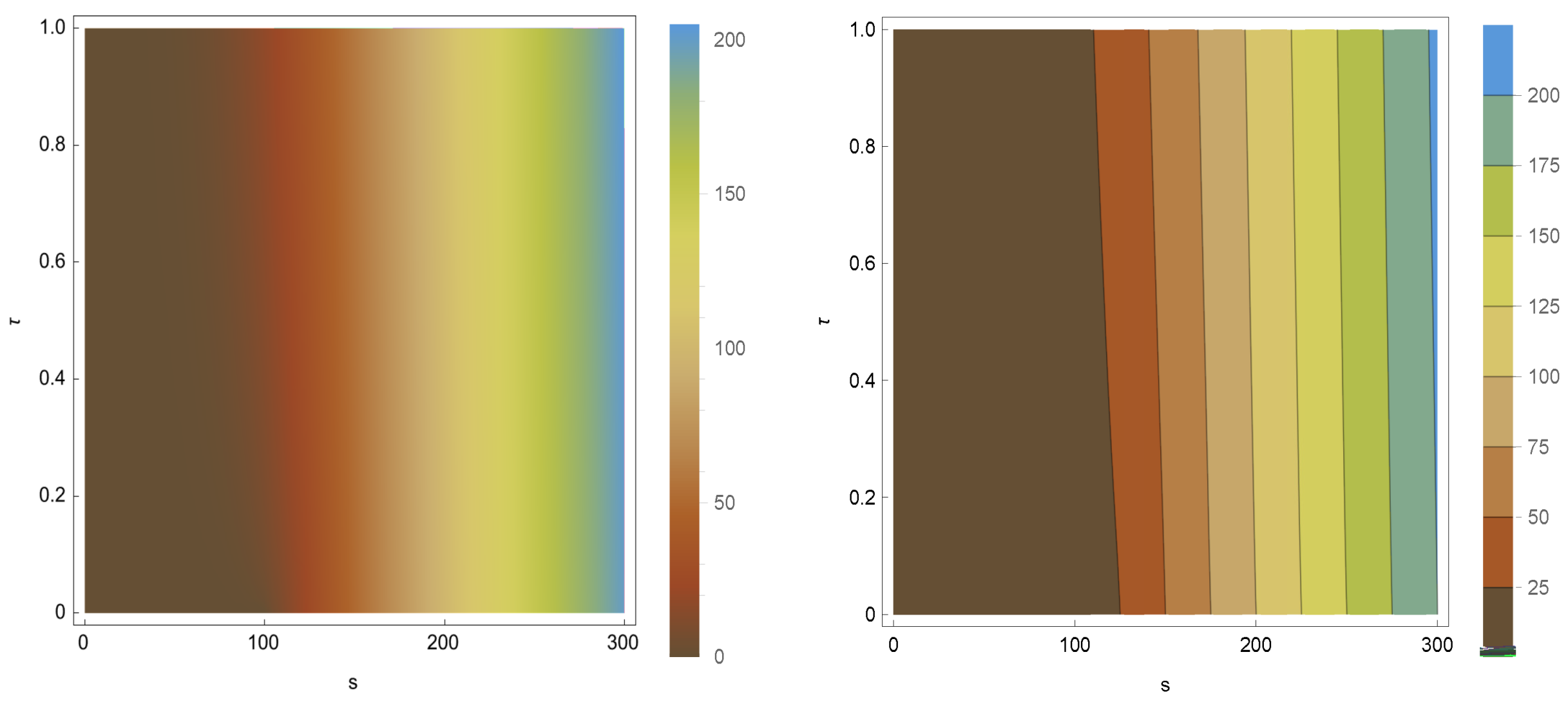
120	18.055	1.3 × ${10}^{-1}$	19.55	18.190	1.6 × ${10}^{-3}$	19.85	18.189	9.45 × ${10}^{-4}$	20.57

offers a detailed comparison of various numerical approaches for solving (3). The proposed solver demonstrates superior performance in terms of both accuracy and computational efficiency. To evaluate the positivity and stability of the developed method, computational results have been analyzed for varying numbers of discretization nodes across the computational area. These results are illustrated in Figure 2, where numerical solutions are presented for two sets of uniformly distributed discretized nodes.

Example 2. 

Consider a put option scenario where the spot/strike price is initially set at 100 USD. The current date is 25 March 2025, with the option scheduled to expire on 25 March 2026. The r is assumed to be 5%, while the annualized volatility is specified as 30%, and the parameter q is taken as 20%. Moreover, for $\alpha =0.7$, a reference price of $b(E,T)\simeq 24.6299$ is obtained, as reported in [33]. This reference value serves as a benchmark for comparative analysis and validation.

The objective of these numerical comparisons is to conduct a comprehensive evaluation of the accuracy, computational efficiency, and overall effectiveness of different numerical schemes applied to this particular problem. By performing these assessments, we aim to obtain a deeper understanding of the strengths and limitations of every method, ultimately refining our understanding of their suitability for tackling the complexities inherent in Example 2. The computational performance of the proposed NS is systematically presented in

Table 2. Outcomes derived from multiple solvers within the scope of Example 2.

N,n	b $\mathit{FDM}$	$\mathit{Error}$ $\mathit{FDM}$	$\mathit{Time}$ $\mathit{FDM}$	b $\mathit{SOS}$	$\mathit{Error}$ $\mathit{SOS}$	$\mathit{Time}$ $\mathit{SOS}$	b $\mathit{NS}$	$\mathit{Error}$ $\mathit{NS}$	$\mathit{Time}$ $\mathit{NS}$
11	23.914	7.1 × ${10}^{-1}$	0.01	23.631	9.9 × ${10}^{-1}$	0.02	23.725	9.0 × ${10}^{-1}$	0.03
21	24.316	3.1 × ${10}^{-1}$	0.03	24.117	5.1 × ${10}^{-1}$	0.04	24.348	2.8 × ${10}^{-1}$	0.05
41	24.466	1.6 × ${10}^{-1}$	0.14	24.356	2.7 × ${10}^{-1}$	0.19	24.650	2.0 × ${10}^{-2}$	0.20
81	24.545	8.4 × ${10}^{-2}$	3.97	24.565	6.4 × ${10}^{-2}$	3.92	24.622	7.9 × ${10}^{-3}$	4.14
161	24.580	4.9 × ${10}^{-2}$	62.77	24.636	6.1 × ${10}^{-3}$	63.14	24.624	5.9 × ${10}^{-3}$	63.58

, providing an analysis of its efficiency.

The specific selection of $\alpha =0.8$ or $\alpha =0.7$ plays a crucial role in this investigation, as it enables an evaluation of the solver’s performance under different fractional derivative values in (3). This approach facilitates a rigorous assessment of the method’s effectiveness across varying Hurst index values within the framework of FBM. By examining these cases, we obtain a comprehensive understanding of the solver’s adaptability across different fractional-order settings, ultimately contributing to a thorough validation of its computational capabilities.

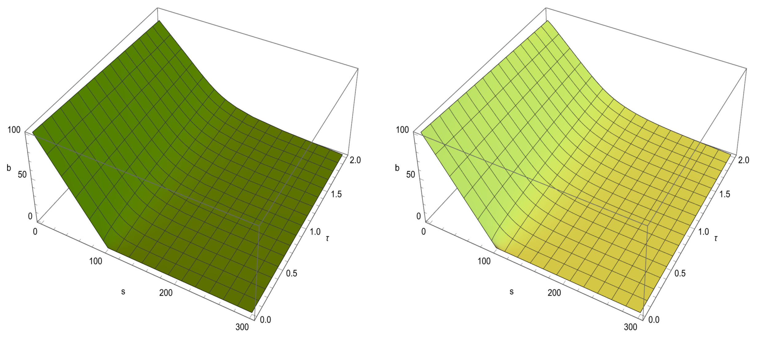
We also draw the solutions of Example 2 using two numerical scheme (FDM and NS) when $N=n=81$. Both solvers show stable behavior; however, the accuracy of NS is higher based on Table 2. The 3D numerical results in Figure 3 further validate the superior accuracy of NS compared to FDM, despite both methods exhibiting stable solutions.

7. Conclusions

The fractional BS PDE represents an advancement over the classical model by incorporating memory effects and non-Brownian characteristics observed in equity markets. By addressing issues such as volatility clustering, heavy-tailed return distributions, and market microstructure noise, this approach provides a more accurate and flexible framework for pricing options. The use of fractional calculus enhances the robustness of option pricing models, making them more suitable for real-world financial applications.

In this work, we have developed a robust and efficient computational scheme for solving the temporal fractional financial option pricing PDE using a novel set of analytically derived weights within a local meshless framework. By leveraging the second integration of a modified MQ RBF, we constructed highly accurate approximations for first and second derivatives, which significantly enhance stability and reduce computational errors. Our numerical experiments have demonstrated the effectiveness of the proposed approach, highlighting its superiority over conventional numerical weights in terms of accuracy and robustness.

Future research directions could focus on extending the proposed method to multidimensional financial PDEs, where the complexity of derivative approximations increases. Additionally, incorporating adaptive mesh refinement techniques could further enhance computational efficiency, especially for problems involving sharp gradients. Exploring alternative basis functions and hybrid methodologies that combine the strengths of analytical and numerical weights may also lead to further improvements in accuracy and stability. Finally, applying this methodology to financial models with stochastic volatility and jump processes could provide valuable insights into its practical applications in finance.