Adsorption–Desorption at Anomalous Diffusion: Fractional Calculus Approach

Abstract

A mathematical model of the anomalous diffusion of surfactant and the process of adsorption–desorption on an interface is analyzed using a fractional calculus approach. The model is based on time-fractional partial differential equations in the bulk phases and the corresponding time-fractional description of the flux bulk–interface. The general case, when the surfactant is soluble in both phases, is considered under the assumption that the adsorption–desorption process is diffusion-controlled. Some of the most popular kinetic models of Henry, Langmuir, and Volmer are considered. Applying the Laplace transform, the partial differential model is transformed into a single multi-term time-fractional nonlinear ordinary differential equation for the surfactant concentration on the interface. Based on existing analytical solutions of linear time-fractional differential equations, the exact solution in the case of the Henry model is derived in terms of multinomial Mittag–Leffler functions, and its asymptotic behavior is studied. Further, the fractional differential model in the general nonlinear case is rewritten as an integral equation, which is a generalization of the well-known Ward–Tordai equation. For computer simulations, based on the obtained integral equation, a predictor–corrector numerical technique is developed. Numerical results are presented and analyzed.

1. Introduction

In the past few decades, fractional-order generalizations of various classical integer-order models have been extensively studied [1,2,3]. In many cases, they enable the achievement of better quantitative agreement with experimental data. The non-local character of fractional derivatives over time makes their use appropriate in the modeling of phenomena, where some hereditary mechanisms are present. In such cases, the physical meaning of the order of the fractional derivative is an index of memory [4].

Regarding the diffusion transport, numerous experimental measurements have reported that the mean squared displacement scales over time as a fractional power law. This deviation from the Markovian description cannot be properly described by the classical diffusion models. Different types of partial differential and integro-differential equations (see, e.g., [5,6]) are used to model such anomalous diffusion processes. In particular, the power law dependence of the mean squared displacement on time can be captured by employing time-fractional derivatives.

In general, anomalous diffusion occurs as a part of a more complex process, see for instance, [7,8,9], where reaction–diffusion systems are studied, refs. [10,11,12] for convection–diffusion models, or [13] for convection-reaction–diffusion systems. Other examples include anomalous diffusion with mass absorption [14], or the adsorption–desorption process at a boundary [15,16,17,18]. Additionally, the diffusion itself can have a complex character, e.g., different properties depending on space directions, as in comb-like models [19]. Different types of fractional derivative operators are used to describe anomalous diffusion [20]. All of the above studies consider fractional generalizations of the classical integer-order models. In the case of complex multi-component systems, the question of the proper “fractionalization” of a classical model is essential and should be performed in such a way that the fundamental conservation and constitutive laws are satisfied. In this respect, as is mentioned in [18], the formulation of boundary conditions is important for the proper description of particle transport to and from a bounding interface.

The surfactants play an essential role in a number of man-made and natural processes. When present on an interface, a surfactant reduces the interfacial tension and introduces important mechanical properties, such as surface elasticity. Adsorption of surfactant on an interface is no less important than the process of diffusion for the dynamics of the surfactant distribution, especially on the interface. The first theoretical result on the dynamics of surfactant interfacial layers is the work of Ward and Tordai (1946) [21]. The Ward–Tordai integral equation is still a basis for most of the theoretical studies that describe the time dependence of the interfacial properties [22]. Fifteen years later, using the Laplace transform, Hansen [23] derives the solution of the same problem as an integro-differential equation. Recently, Hristov [24] pointed out that the Ward–Tordai and Hansen equations are, in fact, fractional integral and differential equations, respectively, of order $1/2$. Thus, the famous Ward–Tordai integral equation and the Hansen integro-differential equation, governing the same problem of the diffusion-controlled adsorption of surfactants at an air–liquid interface, are remarkable examples of a fractional-order equation derived from a classical integer-order model.

The present work extends our previous study [17] on the modeling of surfactant diffusion and the corresponding process of adsorption–desorption by employing fractional derivatives over time. Starting from basic physical concepts (conservation and constitutive laws), a mathematical model is derived, and the behavior of the corresponding solutions is analyzed with the help of computer simulations.

This paper is organized as follows. In Section 2, the time-fractional modeling of anomalous diffusion is discussed in the case when it is a part of a more complex process, regarding mass conservation. In Section 3, a time-fractional model of the anomalous mass-transfer of surfactant, soluble in both phases, is derived in the case when the adsorption–desorption process is controlled by diffusion. Section 4 is devoted to the linear case of the Henry adsorption isotherm and contains a detailed analysis, which is mainly based on the theory of multinomial Mittag–Leffler functions. In Section 5, a numerical approach is proposed for the general nonlinear case, and some numerical results are presented. A discussion and conclusions can be found in Section 6.

2. Time-Fractional Diffusion–Adsorption Model

In the present section, we assess a generalization of the classical diffusion equation and the related boundary conditions of adsorption–desorption to anomalous ones. The assessment is based on basic physical principles and laws. The classical model of the mass transfer of species of concentration C in a fluid medium consists of two parts. The first part is the continuity equation, which, in the case of a concentration problem, guarantees mass conservation. It is written below in a general form, including diffusion, convection, and reaction terms:

$${\displaystyle \frac{\partial C}{\partial t}}=-\nabla ·\mathbf{J}(\mathbf{x},t)-\nabla ·{\mathbf{J}}_{conv}(\mathbf{x},t)+g(C,\mathbf{x},t),$$

(1)

where ∇ denotes the gradient vector, $\mathbf{J}(\mathbf{x},t)$ and ${\mathbf{J}}_{conv}(\mathbf{x},t)$ are the diffusive and convective fluxes, respectively, and $g(C,\mathbf{x},t)$ takes into account the change of concentration due to source or reaction (e.g., chemical or biological).

The second part of the model consists of constitutive equations that describe the different processes under consideration. In the case of the process of diffusion, the constitutive equation for the diffusive flux $\mathbf{J}$ is given by Fick’s first law:

$$\mathbf{J}(\mathbf{x},t)=-d\nabla C(\mathbf{x},t),$$

(2)

where d is the diffusion coefficient. As a part of the diffusive flux, drift due to an external force can be considered (see, e.g., [15,25,26]). Such is also the electrodiffusion flux in the case of ionic surfactant subjected to an external electromagnetic field (see [27]).

Convection can be introduced into the model in different ways, for instance, via the convective flux:

$${\mathbf{J}}_{conv}(\mathbf{x},t)=\mathbf{u}(x,t)C(\mathbf{x},t).$$

(3)

Here, $\mathbf{u}$ is the fluid velocity, which is external to the diffusion equation.

The first question regarding time fractional diffusion models is how to introduce the fractional operators. In general, there are two main approaches. In the first approach, a fractional derivative ${\mathbb{D}}_t^{\alpha }$ replaces the first time derivative in the left-hand side of the continuity Equation (1), which implies

$${\mathbb{D}}_t^{\alpha }C(\mathbf{x},t)=-\nabla ·\mathbf{J}(\mathbf{x},t)-\nabla ·{\mathbf{J}}_{conv}(\mathbf{x},t)+g(C,\mathbf{x},t).$$

(4)

Most studies of time-fractional diffusion use this approach, see e.g., [8,10,11,12,13,14,16,28]. There are, however, some issues that arise when using this approach. The first is in the case when more than one different processes are considered. Indeed, then (4) leads to the illogical conclusion that all subprocesses described by the terms in the right-hand side have a fractional evolution of one and the same order, $\alpha$. Another issue is related to the fact that the continuity equation represents the mass conservation of C, and a change of (1) could lead to a violation of the mass conservation law. For instance, if only convective flux is present in the right-hand side of (1) and the velocity $\mathbf{u}$ is not constant, mass conservation would be satisfied only if ${\mathbb{D}}_t^{\alpha }$ is the first order derivative.

In the second approach, a fractional operator is used in the description of a given process (e.g., diffusion or reaction) via the corresponding constitutive equation (e.g., (2) or g(C,x,t)). In the case of anomalous diffusion, this is:

$$\mathbf{J}(\mathbf{x},t)=-d_{\alpha }{D}_t^{1-\alpha }\nabla C(\mathbf{x},t),0<\alpha <1,$$

(5)

see e.g., [7,9,19,26,29]. It is worth mentioning that the issues discussed above regarding the first approach are not present here. That is why we use the model of anomalous diffusion via the diffusive flux (5). Let us note that the two approaches are equivalent when only diffusion is considered, i.e., $J_{conv}=0$ and $g(C,\mathbf{x},t)=0$ (see [30]).

The second question is: What kind of fractional operator is appropriate for modeling adsorption–desorption at anomalous diffusion? In a mathematical model, all terms of a given equation or boundary condition must have the same physical dimension. In order to guarantee this, in the equation for the anomalous diffusive flux (5), the dimension of the fractional diffusion coefficient $d_{\alpha }$ is chosen to correspond to the dimension of the fractional differential operator. Thus, a requirement on the fractional operator $D_t^{\alpha }$ is to have a well-defined physical dimension.

In the present study, as in [15], fractional operators of the Riemann–Liouville type are used. The main argument for the choice of Riemann–Liouville operators is the fact that the solution of the classical adsorption–diffusion model is given in the Ward–Tordai equation by the Riemann–Liouville fractional integral of order $1/2$.

Recall that the Riemann–Liouville fractional integral $I_t^{\alpha }$ is defined by

$$I_t^{\alpha }u\left(t\right)={\displaystyle \frac{1}{\Gamma \left(\alpha \right)}}{\int }_0^{t}u\left(\tau \right){(t-\tau )}^{\alpha -1}\mathrm{d}\tau ,\alpha >0.$$

(6)

The Riemann–Liouville fractional derivative $D_t^{\alpha }$ of order $\alpha \in (0,1)$ is:

$$D_t^{\alpha }u\left(t\right)={\displaystyle \frac{1}{\Gamma (1-\alpha )}}{\displaystyle \frac{\mathrm{d}}{\mathrm{d}t}}{\int }_0^t{\displaystyle \frac{u\left(\tau \right)}{{(t-\tau )}^{\alpha }}}\mathrm{d}\tau ,\alpha \in (0,1).$$

(7)

The operators $D_t^{\alpha }$ and $I_t^{\alpha }$ have dimensions [$tim{e}^{-\alpha }$] and [$tim{e}^{\alpha }$], respectively. In other words, if the time is rescaled as $t=T.\tilde{t}$, then:

$$D_t^{\alpha }=T^{-\alpha }{D}_{\tilde{t}}^{\alpha },I_t^{\alpha }=T^{\alpha }{I}_{\tilde{t}}^{\alpha },t=T.\tilde{t}.$$

(8)

By proper choice of the characteristic time T, the above rescaling is used to render the mathematical model dimensionless and to reduce the number of parameters. In [20], the authors also consider some non-singular fractional operators for the modeling of anomalous diffusion. They, however, do not have a physical dimension. It is claimed in [31] that the Caputo–Fabrizio fractional derivative of order $\alpha$ has dimension $tim{e}^{-\alpha }$. This fractional derivative, however, does not satisfy (8).

Together with diffusion, adsorption also plays an important role in the process of surfactant transport in multiphase fluid systems. The adsorption process at an interface $S=\partial \Omega$ is described by the boundary condition:

$${\left.{\displaystyle \frac{\partial G}{\partial t}}\right|}_S=-\mathbf{J}·\mathbf{n}\mathrm{on}S,$$

(9)

where G is the surfactant concentration on the interface S, $\mathbf{n}$ is the inward for $\Omega$ unit vector, which is normal to S, and $\mathbf{J}$ is the flux in the bulk phase $\Omega$. The boundary condition (9) represents mass conservation of the surfactant in the vicinity of the interface S. In the second approach adopted here, the flux $\mathbf{J}$ is given by Equation (5) and the fractional derivative generalization of the classical diffusion–adsorption model reads:

$${\displaystyle \frac{\partial C}{\partial t}}=d_{\alpha }{D}_t^{1-\alpha }\Delta C(\mathbf{x},t),{\left.{\displaystyle \frac{\partial G}{\partial t}}\right|}_S=d_{\alpha }{D}_t^{1-\alpha }\nabla C·\mathbf{n}.$$

(10)

Thus, the time-fractional derivatives in the diffusion equation and adsorption boundary condition are the same (see also [18]). This means that the flux bulk-interface is the same as that in the continuous phase $\Omega$, which guarantees mass conservation (see [15]).

Relatedly, let us point out that the boundary condition on the interface in our previous work [17] is incorrect.

3. Mathematical Formulation

In this section, the mathematical model of the diffusion-controlled adsorption of surfactant at the liquid–liquid interface is discussed in the one-dimensional case, assuming anomalous diffusion in both liquid phases. The model is based on Equations (5) and (10).

Consider a surfactant that is soluble in two liquid phases. The two phases are in contact at an interface. Such a system is, in general, not in equilibrium, and surfactant diffusion processes in the bulk phases and adsorption on the interface take place.

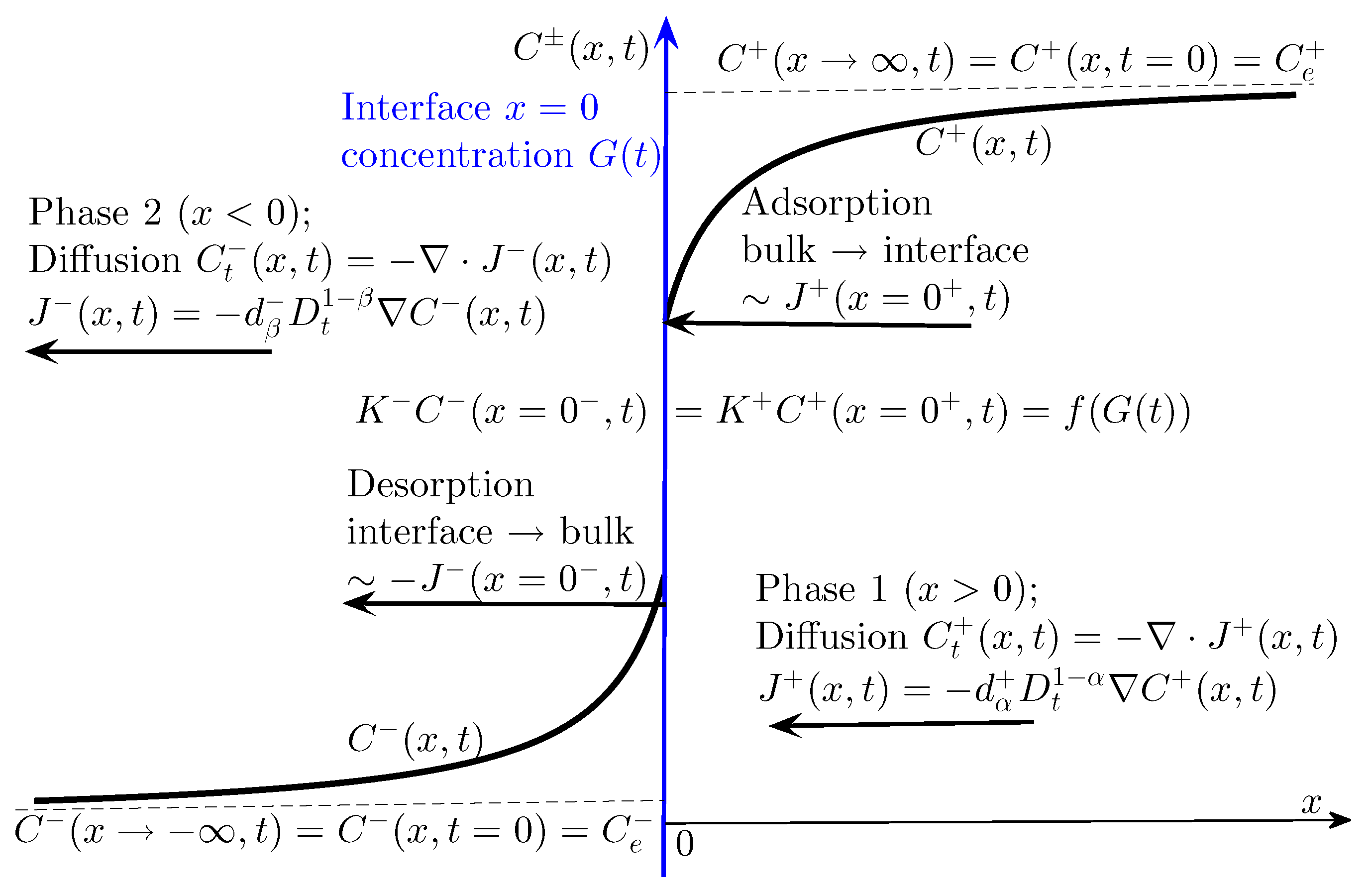
A schematic sketch of the problem for diffusion-controlled adsorption at the liquid–liquid interface is given in Figure 1, where $C^{+}(x,t)$ and $C^{-}(x,t)$ denote the surfactant concentrations in Phase 1 ($x>0$) and Phase 2 ($x<0$), respectively; $G\left(t\right)$ is the concentration of surfactant on the interface, and $x=0$ and $K^{\pm }$ are adsorption constants.

The mathematical formulation of the problem for adsorption at the liquid–liquid interface controlled by anomalous diffusion contains two time-fractional equations for the anomalous diffusion of surfactant in the bulk phases:

$$\begin{array}{ccc}& & {\displaystyle \frac{\partial C^{+}(x,t)}{\partial t}}=d_{\alpha }^{+}{D}_t^{1-\alpha }{\displaystyle \frac{{\partial }^2{C}^{+}(x,t)}{\partial x^2}},x>0,\hfill \end{array}$$

(11)

$$\begin{array}{ccc}& & {\displaystyle \frac{\partial C^{-}(x,t)}{\partial t}}=d_{\beta }^{-}{D}_t^{1-\beta }{\displaystyle \frac{{\partial }^2{C}^{-}(x,t)}{\partial x^2}},x<0,\hfill \end{array}$$

(12)

where $\alpha$ and $\beta$ are parameters of anomalous diffusion, $0<\alpha ,\beta \le 1$, and $d_{\alpha }^{+}$, $d_{\beta }^{-}$ are diffusion coefficients in the corresponding phases. The above diffusion equations are complemented with the initial conditions of uniform surfactant distribution at $t=0$:

$$C^{+}(x,0)=C_e^{+},x>0;C^{-}(x,0)=C_e^{-},x<0,$$

(13)

where $C_e^{\pm }$ are the input concentrations of surfactant in the bulk phases. Without loss of generality, we assume $C_e^{+}\ge C_e^{-}$. The boundary conditions are

$$\underset{x\to \pm \infty }{lim}{C}^{\pm }(x,t)=C_e^{\pm },\underset{x\to 0^{\pm }}{lim}{C}^{\pm }(x,t)=C_s^{\pm }\left(t\right),t>0,$$

(14)

where $C_s^{\pm }\left(t\right)$ are the subsurface surfactant concentrations. The following identities for the two subsurface surfactant concentrations are satisfied:

$$K^{-}{C}_s^{-}\left(t\right)=K^{+}{C}_s^{+}\left(t\right)=f\left(G\left(t\right)\right),t>0,$$

(15)

where the function $f(·)$ is the so-called adsorption isotherm. Different adsorption isotherms are considered in the literature [27]. In the present study, three of the most popular models are used. The corresponding definitions of $f\left(G\right)$ are given in

Table 1. Expressions for $f\left(G\right)$ for the considered kinetic models.

Adsorption Isotherm	Function $\mathit{f}\left(\mathit{G}\right)$
Henry	${\displaystyle f\left(G\right)=G/G_{\infty }}$
Langmuir	${\displaystyle f\left(G\right)=\frac{G/G_{\infty }}{1-G/G_{\infty }}}$
Volmer	${\displaystyle f\left(G\right)=\frac{G/G_{\infty }}{1-G/G_{\infty }}exp\left(\frac{G/G_{\infty }}{1-G/G_{\infty }}\right)}$

, where the parameter $G_{\infty }$ is the maximum possible surfactant concentration.

The change of the surfactant concentration $G\left(t\right)$ on the interface is compensated for by the diffusion fluxes from the bulk phases, resulting in the equation

$${\displaystyle \frac{dG\left(t\right)}{dt}}=d_{\alpha }^{+}{D}_t^{1-\alpha }{\left.{\displaystyle \frac{\partial C^{+}(x,t)}{\partial x}}\right|}_{x=0^{+}}-d_{\beta }^{-}{D}_t^{1-\beta }{\left.{\displaystyle \frac{\partial C^{-}(x,t)}{\partial x}}\right|}_{x=0^{-}},t>0,$$

(16)

with initial condition $G\left(0\right)=G_0$, where $G_0$ is the initial surfactant concentration on the interface.

The problem is treated by applying the Laplace transform with respect to time variable t, where the following notations are used:

$$\mathcal{L}\left\{u(x,t)\right\}\left(s\right)=\widehat{u}(x,s)={\int }_0^{\infty }{e}^{-st}u(x,t)dt.$$

The Laplace transform pairs for fractional order integration and differentiation are

$$\mathcal{L}\left\{D_t^{\alpha }f\right\}\left(s\right)=s^{\alpha }\widehat{f}\left(s\right),\alpha \in (0,1),$$

(17)

which can be derived from the identity

$$\mathcal{L}\left\{{\displaystyle \frac{t^{\alpha -1}}{\Gamma \left(\alpha \right)}}\right\}=s^{-\alpha },\alpha >0,$$

(18)

and the relation for the first order derivative $\mathcal{L}\left\{f^{\prime }\right\}\left(s\right)=s\widehat{f}\left(s\right)-f\left(0\right)$.

To find an equation for the surfactant concentration on the interface $G\left(t\right)$, we first apply the Laplace transform with respect to variable t to the diffusion Equations (11) and (12) by the use of relation (17). Taking into account the initial conditions (13), the following identities in the Laplace domain are derived:

$$\begin{array}{ccc}& & s\widehat{C^{+}}(x,s)-C_e^{+}=d_{\alpha }^{+}{s}^{1-\alpha }{\displaystyle \frac{{\partial }^2\widehat{C^{+}}}{\partial x^2}},x>0,\hfill \\ & & s\widehat{C^{-}}(x,s)-C_e^{-}=d_{\beta }^{+}{s}^{1-\beta }{\displaystyle \frac{{\partial }^2\widehat{C^{-}}}{\partial x^2}},x<0.\hfill \end{array}$$

These two equations in x, with s considered as a parameter, are equipped with boundary conditions for $\widehat{C^{\pm }}(x,s)$, derived from conditions (14): $\widehat{C^{\pm }}(0,s)={\widehat{C^{\pm }}}_s\left(s\right),\widehat{C^{\pm }}(\pm \infty ,s)=C_e^{\pm }/s$. Their solutions are

$$\begin{array}{ccc}& & \widehat{C^{+}}(x,s)={\displaystyle \frac{C_e^{+}}{s}}+\left(\widehat{C_s^{+}}\left(s\right)-{\displaystyle \frac{C_e^{+}}{s}}\right)exp\left(-x\sqrt{{\displaystyle \frac{s^{\alpha }}{d_{\alpha }^{+}}}}\right),x>0,\hfill \end{array}$$

(19)

$$\begin{array}{ccc}& & \widehat{C^{-}}(x,s)={\displaystyle \frac{C_e^{-}}{s}}+\left(\widehat{C_s^{-}}\left(s\right)-{\displaystyle \frac{C_e^{-}}{s}}\right)exp\left(x\sqrt{{\displaystyle \frac{s^{\beta }}{d_{\beta }^{-}}}}\right),x<0.\hfill \end{array}$$

(20)

Further, application of the Laplace transform to Equation (16) yields

$$s\widehat{G}\left(s\right)-G_0=d_{\alpha }^{+}{s}^{1-\alpha }{\left.{\displaystyle \frac{\partial \widehat{C^{+}}}{\partial x}}\right|}_{x=0^{+}}-d_{\beta }^{-}{s}^{1-\beta }{\left.{\displaystyle \frac{\partial \widehat{C^{-}}}{\partial x}}\right|}_{x=0^{-}},$$

which, by the use of relations (19) and (20), implies

$$s\widehat{G}\left(s\right)-G_0=\sqrt{d_{\alpha }^{+}}{s}^{1-\alpha /2}\left({\displaystyle \frac{C_e^{+}}{s}}-\widehat{C_s^{+}}\left(s\right)\right)+\sqrt{d_{\beta }^{-}}{s}^{1-\beta /2}\left({\displaystyle \frac{C_e^{-}}{s}}-\widehat{C_s^{-}}\left(s\right)\right).$$

(21)

In order to obtain a fractional differential equation for $G\left(t\right)$ in a form convenient for applications, we rewrite (21) as follows:

$$s\widehat{G}\left(s\right)-G_0+\sqrt{d_{\alpha }^{+}}{s}^{1-\alpha /2}\widehat{C_s^{+}}\left(s\right)+\sqrt{d_{\beta }^{-}}{s}^{1-\beta /2}\widehat{C_s^{-}}\left(s\right)=\sqrt{d_{\alpha }^{+}}{s}^{-\alpha /2}{C}_e^{+}+\sqrt{d_{\beta }^{-}}{s}^{-\beta /2}{C}_e^{-}.$$

Then, the application of the inverse Laplace transform yields, by the use of (17) and (18),

$$G^{\prime }\left(t\right)+\sqrt{d_{\alpha }^{+}}{D}_t^{1-\alpha /2}{C}_s^{+}\left(t\right)+\sqrt{d_{\beta }^{-}}{D}_t^{1-\beta /2}{C}_s^{-}\left(t\right)=H\left(t\right),$$

where $G^{\prime }\left(t\right)$ denotes, as usual, the first derivative of $G\left(t\right)$ and

$$H\left(t\right)=\sqrt{d_{\alpha }^{+}}{C}_e^{+}{\displaystyle \frac{t^{\alpha /2-1}}{\Gamma (\alpha /2)}}+\sqrt{d_{\beta }^{-}}{C}_e^{-}{\displaystyle \frac{t^{\beta /2-1}}{\Gamma (\beta /2)}}.$$

(22)

Taking into account identities (15) for the subsurface surfactant concentrations $C_s^{\pm }\left(t\right)$, we obtain the following multi-term fractional differential equation for $G\left(t\right)$:

$$G^{\prime }\left(t\right)+{\displaystyle \frac{\sqrt{d_{\alpha }^{+}}}{K^{+}}}{D}_t^{1-\alpha /2}f\left(G\left(t\right)\right)+{\displaystyle \frac{\sqrt{d_{\beta }^{-}}}{K^{-}}}{D}_t^{1-\beta /2}f\left(G\left(t\right)\right)=H\left(t\right),t>0,$$

(23)

with initial condition $G\left(0\right)=G_0$, where $H\left(t\right)$ is defined in (22).

Let us note that the derived Equation (23) is well defined for parameters $\alpha$ and $\beta$ in a larger interval, namely $0<\alpha ,\beta \le 2$. In this way, we can cover different diffusive regimes, depending on the values of the fractional parameters $\alpha$ and $\beta$. Recall that for a fractional parameter $\alpha$, the case $0<\alpha <1$ corresponds to subdiffusion, $1<\alpha <2$ cover the superdiffusive regime, and $\alpha =2$ corresponds to a ballistic diffusion process; see, e.g., [30]. In the case when $\alpha >1$ or $\beta >1$ in the initial Equations (11), (12) and (16), then the fractional derivative $D_t^{1-\alpha }$ (resp. $D_t^{1-\beta }$) is replaced by a fractional integral $I_t^{\alpha -1}$ (resp. $I_t^{\beta -1}$). In view of the above argument, in this work, we consider the whole region $0<\alpha ,\beta \le 2$.

Let us point out that, in the case of classical diffusion $\alpha =\beta =1$, Equation (23) reduces to a fractional order equation of the form $G^{\prime }\left(t\right)+c{D}_t^{1/2}f\left(G\left(t\right)\right)=H\left(t\right)$. In this case, a classical integer-order problem leads to a problem of fractional order for $G\left(t\right)$.

For the presentation of the results and their analysis transformation of the surfactant concentration G and the time t is performed next. It renders the governing Equation (23) dimensionless and leads to a reduction of the parameters of the problem. The transformed variables $\tilde{G}$ and $\tilde{t}$ are, respectively,

$$\begin{array}{ccc}\hfill \tilde{G}& =& G/G_e,\hfill \end{array}$$

(24)

$$\begin{array}{ccc}\hfill \tilde{t}& =& t/T,T={\left[{\displaystyle \frac{K^{+}{G}_{\infty }}{\sqrt{d_{\alpha }^{+}}}}\right]}^{2/\alpha }=a^{-2/\alpha }.\hfill \end{array}$$

(25)

In the above transformation, T is the characteristic anomalous diffusion time and $G_e$ is the equilibrium surfactant concentration, which is defined based on the parameters in Phase 1 from the equation

$$K^{+}{C}_e^{+}=f\left(G_e\right).$$

(26)

For any of the adsorption isotherms given in Table 1, there is exactly one solution $G_e$ satisfying (26). In the present study, $G_e$ is used as a characteristic surfactant concentration on the interface (note that $0\le G\left(t\right)\le G_e$).

Using (8), we apply the transformations (24) and (25) to the governing Equation (23). For simplicity, we restrict our considerations to a practically more interesting case when the surfactant is initially present only in one of the phases (e.g., in Phase 1, i.e., $C_e^{-}=0$). Then, Equation (23) takes the following dimensionless form:

$${\tilde{G}}^{\prime }\left(\tilde{t}\right)+D_{\tilde{t}}^{1-\alpha /2}\tilde{f}\left(\tilde{G}\left(\tilde{t}\right)\right)+B{D}_{\tilde{t}}^{1-\beta /2}\tilde{f}\left(\tilde{G}\left(\tilde{t}\right)\right)=\tilde{f}\left(1\right){\displaystyle \frac{{\tilde{t}}^{\alpha /2-1}}{\Gamma (\alpha /2)}},\tilde{G}\left(0\right)={\tilde{G}}_0=G_0/G_e,$$

(27)

where the dimensionless group B and the transformed function $\tilde{f}$ are defined as:

$$B=\sqrt{{\displaystyle \frac{d_{\beta }^{-}}{d_{\alpha }^{+}}}}{\displaystyle \frac{K^{+}}{K^{-}}}{\left[{\displaystyle \frac{K^{+}{G}_{\infty }}{\sqrt{d_{\alpha }^{+}}}}\right]}^{\beta /\alpha -1},\tilde{f}\left(u\right)=f\left(u{G}_e\right)G_{\infty }/G_e.$$

Let us note that for all considered adsorption isotherms the terms $\tilde{f}\left(u\right)$ and $\tilde{f}\left(1\right)$ depend on one parameter and that is the transformed maximum possible surfactant concentration ${\tilde{G}}_{\infty }=G_{\infty }/G_e$. Thus, the parameters of the dimensionless governing Equation (27) are four: $\alpha$, $\beta$, B, and ${\tilde{G}}_{\infty }$.

The Henry kinetic model plays an important role in the theoretical investigation of surfactant adsorption–desorption. It can serve as a base for a second-order approximation of the nonlinear models, which will be discussed later. That is why the following section is devoted to the derivation of an analytical solution in the case of the Henry adsorption isotherm and a theoretical analysis of its behavior.

4. The Case of Henry Adsorption Isotherm

In the simplest case of the Henry isotherm, the function f is linear and Equation (23) is a linear multi-term fractional equation for $G\left(t\right)$, the solution of which admits explicit representation in terms of a multinomial Mittag–Leffler function. The solution can be studied analytically based on the properties of this special function. The definition and relevant properties of the multinomial Mittag–Leffler function are summarized next.

4.1. Multinomial Mittag–Leffler Function

The multinomial Mittag–Leffler function of two variables is defined as follows (see, e.g., [32,33]):

$$E_{({\mu }_1,{\mu }_2),\nu }(z_1,z_2)=\sum _{k=0}^{\infty }\sum _{l=0}^{\infty }{\displaystyle \frac{(k+l)!}{k!l!}}{\displaystyle \frac{z_1^k{z}_2^l}{\Gamma \left(\nu +{\mu }_{1}k+{\mu }_{2}l\right)}},$$

(28)

where $z_1,z_2\in \mathbb{C},{\mu }_1,{\mu }_2,\nu \in \mathbb{R}$, ${\mu }_1>0,{\mu }_2>0$.

Let us note that the commutativity identity $E_{({\mu }_1,{\mu }_2),\nu }(z_1,z_2)=E_{({\mu }_2,{\mu }_1),\nu }(z_2,z_1)$ is satisfied. If one of the variables vanishes, Function (28) reduces to the classical Mittag–Leffler function, i.e.,

$$E_{({\mu }_1,{\mu }_2),\nu }(z,0)=E_{{\mu }_1,\nu }\left(z\right)=\sum _{k=0}^{\infty }{\displaystyle \frac{z^k}{\Gamma \left(\nu +{\mu }_{1}k\right)}}.$$

(29)

Of particular interest is the multinomial Mittag–Leffler type function,

$${\mathcal{E}}_{({\mu }_1,{\mu }_2),\nu }\left(t\right)=t^{\nu -1}{E}_{({\mu }_1,{\mu }_2),\nu }(-{\lambda }_1{t}^{{\mu }_1},-{\lambda }_2{t}^{{\mu }_2}),$$

(30)

where ${\lambda }_1,{\lambda }_2\in \mathbb{R}$, $t>0$, since it admits the following simple Laplace transform:

$$\mathcal{L}\left\{{\mathcal{E}}_{({\mu }_1,{\mu }_2),\nu }\left(t\right)\right\}\left(s\right)={\displaystyle \frac{s^{-\nu }}{1+{\lambda }_1{s}^{-{\mu }_1}+{\lambda }_2{s}^{-{\mu }_2}}}.$$

(31)

In this work, we will need the integration rule [33]

$$I_t^{\delta }\left({\mathcal{E}}_{({\mu }_1,{\mu }_2),\nu }\left(t\right)\right)={\int }_0^t{g}_{\delta }(t-\tau ){\mathcal{E}}_{({\mu }_1,{\mu }_2),\nu }\left(\tau \right)d\tau ={\mathcal{E}}_{({\mu }_1,{\mu }_2),\nu +\delta }\left(t\right),\delta >0,$$

(32)

where we have used the notation

$$g_{\delta }\left(t\right)={\displaystyle \frac{t^{\delta -1}}{\Gamma \left(\delta \right)}},\delta >0.$$

(33)

For the asymptotic expansions of Function (30), next we assume ${\mu }_1>{\mu }_2$. The first terms in the power series definition (28) give the following asymptotic expansion for small times:

$${\mathcal{E}}_{({\mu }_1,{\mu }_2),\nu }\left(t\right)\sim {\displaystyle \frac{t^{\nu -1}}{\Gamma \left(\nu \right)}}-{\lambda }_2{\displaystyle \frac{t^{\nu +{\mu }_2-1}}{\Gamma (\nu +{\mu }_2)}},t\to 0.$$

(34)

The asymptotic expansion for large t is derived in [33] as follows:

$${\mathcal{E}}_{({\mu }_1,{\mu }_2),\nu }\left(t\right)\sim \left\{\begin{array}{c}{\displaystyle \frac{t^{\nu -{\mu }_1-1}}{{\lambda }_1\Gamma (\nu -{\mu }_1)},{\mu }_1\ne \nu ,}\hfill \\ {\displaystyle -\frac{{\lambda }_2{t}^{-{\mu }_1+{\mu }_2-1}}{{\lambda }_1^2\Gamma (-{\mu }_1+{\mu }_2)},{\mu }_1=\nu ,}\hfill \end{array}\right.t\to +\infty ,$$

(35)

provided that ${\mu }_1>{\mu }_2$.

A function $\varphi :{\mathbb{R}}_{+}\to \mathbb{R}$ is said to be a completely monotone function if it is of class $C^{\infty }$ and

$${(-1)}^n{\varphi }^{\left(n\right)}\left(t\right)\ge 0,t>0,n=0,1,2,\dots$$

(36)

A nonnegative function of class $C^{\infty }$ is a Bernstein function if its first derivative is completely monotone.

For the multinomial Mittag–Leffler type function, it is proved in [33] that if ${\lambda }_1,{\lambda }_2>0$ and

$$0<{\mu }_j\le 1,0<{\mu }_j\le \nu \le 1,j=1,2,$$

(37)

then ${\mathcal{E}}_{({\mu }_1,{\mu }_2),\nu }\left(t\right)$ is completely monotone.

4.2. Representation of the Solution

In the case of the Henry adsorption isotherm, $f\left(G\right)=G/G_{\infty }$ and, therefore, Equation (23) for $G\left(t\right)$ admits the form

$$G^{\prime }\left(t\right)+a{D}_t^{1-\alpha /2}G\left(t\right)+b{D}_t^{1-\beta /2}G\left(t\right)=a_1{\displaystyle \frac{t^{\alpha /2-1}}{\Gamma (\alpha /2)}}+b_1{\displaystyle \frac{t^{\beta /2-1}}{\Gamma (\beta /2)}},G\left(0\right)=G_0,$$

(38)

where

$$a={\displaystyle \frac{\sqrt{d_{\alpha }^{+}}}{K^{+}{G}_{\infty }}},b={\displaystyle \frac{\sqrt{d_{\beta }^{-}}}{K^{-}{G}_{\infty }}},a_1=\sqrt{d_{\alpha }^{+}}{C}_e^{+},b_1=\sqrt{d_{\beta }^{-}}{C}_e^{-}.$$

(39)

Denote by $H\left(t\right)$ the right-hand side of Equation (38),

$$H\left(t\right)=a_1{g}_{\alpha /2}\left(t\right)+b_1{g}_{\beta /2}\left(t\right),$$

where the notation (33) is used. The solution of Equation (38) admits the representation (see [33])

$$G\left(t\right)=G_{0}u\left(t\right)+{\int }_0^{t}u(t-\tau )H\left(\tau \right)d\tau ,$$

(40)

where $u\left(t\right)$ is the solution of the corresponding homogeneous equation

$$u^{\prime }\left(t\right)+a{D}_t^{1-\alpha /2}u\left(t\right)+b{D}_t^{1-\beta /2}u\left(t\right)=0,u\left(0\right)=1.$$

(41)

Applying the Laplace transform and taking into account (17) and (31), the solution of (41) is expressed by the following multinomial Mittag–Leffler type function:

$$u\left(t\right)=E_{(\alpha /2,\beta /2),1}\left(-a{t}^{\alpha /2},-b{t}^{\beta /2}\right).$$

Inserting this result in (40), by applying relation (32), we obtain the solution of (38) as follows:

$$\begin{array}{ccc}\hfill G\left(t\right)& =& G_0{E}_{(\alpha /2,\beta /2),1}\left(-a{t}^{\alpha /2},-b{t}^{\beta /2}\right)\hfill \\ & +& a_1{t}^{\alpha /2}{E}_{(\alpha /2,\beta /2),\alpha /2+1}\left(-a{t}^{\alpha /2},-b{t}^{\beta /2}\right)\hfill \\ & +& b_1{t}^{\beta /2}{E}_{(\alpha /2,\beta /2),\beta /2+1}\left(-a{t}^{\alpha /2},-b{t}^{\beta /2}\right).\hfill \end{array}$$

(42)

Let us consider some particular cases. First, if $\alpha =\beta$, using classical Mittag–Leffler functions, expression (42) reduces to the following:

$$G\left(t\right)=G_0{E}_{\alpha /2,1}\left(-(a+b)t^{\alpha /2}\right)+(a_1+b_1)t^{\alpha /2}{E}_{\alpha /2,\alpha /2+1}\left(-(a+b)t^{\alpha /2}\right).$$

(43)

Here, we have used the identity

$$E_{(\mu ,\mu )\nu }\left(-a{t}^{\mu },-b{t}^{\mu }\right)=E_{\mu ,\nu }\left(-(a+b)t^{\mu }\right),$$

which can be established directly from the power series definitions of the functions or by using the Laplace transform pair (31).

Another particular case is when the surfactant is soluble in only one of the phases (suppose this is Phase 1). Then, $d_{\beta }^{-}=0$, i.e., $b=b_1=0$, and (42) reduces by the use of (29) to

$$G\left(t\right)=G_0{E}_{\alpha /2,1}\left(-a{t}^{\alpha /2}\right)+a_1{t}^{\alpha /2}{E}_{\alpha /2,\alpha /2+1}\left(-a{t}^{\alpha /2}\right).$$

(44)

Let us note that a similarity between expressions (43) and (44) is observed.

Next, we consider in more detail another practically important particular case:

$$G_0=0,C_e^{-}=0,$$

(45)

that is, the case when the interface, as well as one of the phases (Phase 2), is initially free of surfactant.

Further considerations are devoted to the case (45), in which $G_0=b_1=0$ and the solution (42) reduces to

$$G\left(t\right)=a_1{t}^{\alpha /2}{E}_{(\alpha /2,\beta /2),\alpha /2+1}\left(-a{t}^{\alpha /2},-b{t}^{\beta /2}\right).$$

(46)

Based on the asymptotic expansions (34) and (35) of the multinomial Mittag–Leffler type function, we deduce for the solution (46),

$$G\left(t\right)\sim a_1{\displaystyle \frac{t^{\alpha /2}}{\Gamma (\alpha /2+1)}}-a_{1}b{\displaystyle \frac{t^{\alpha /2+\delta /2}}{\Gamma (\alpha /2+\delta /2+1)}},t\to 0^{+},\delta =min\{\alpha ,\beta \},$$

(47)

and

$$G\left(t\right)\sim \left\{\begin{array}{c}{\displaystyle \frac{a_1}{a}=C_e^{+}{K}^{+}{G}_{\infty },\alpha >\beta ,}\hfill \\ {\displaystyle \frac{a_1{t}^{\alpha /2-\beta /2}}{b\Gamma \left(\alpha /2-\beta /2+1\right)}\to 0,\alpha <\beta ,}\hfill \end{array}\right.t\to +\infty .$$

(48)

If $\alpha =\beta$, then (46) reduces to $G\left(t\right)=a_1{t}^{\alpha /2}{E}_{\alpha /2,\alpha /2+1}\left(-(a+b)t^{\alpha /2}\right)$, and the asymptotic expression

$$G\left(t\right)\sim {\displaystyle \frac{a_1}{a+b}},t\to +\infty$$

can be derived from the asymptotics of the classical Mittag–Leffler function $E_{\alpha ,\beta }(-x)\sim x^{-1}/\Gamma (\beta -\alpha )$, $x\to +\infty$.

According to relation (32), the solution (46) admits the integral representation

$$G\left(t\right)=a_1{\int }_0^t{\tau }^{\alpha /2-1}{E}_{(\alpha /2,\beta /2),\alpha /2}\left(-a{\tau }^{\alpha /2},-b{\tau }^{\beta /2}\right)d\tau .$$

(49)

If $\alpha >\beta$, then the function under the integral sign in (49) is completely monotone (since its parameters satisfy the sufficient conditions (37) for complete monotonicity). Therefore, in this case, $G\left(t\right)$ is a Bernstein function. In particular, it is nonnegative, increasing, and concave, and takes values from 0 at $t\to 0^{+}$ to $C_e^{+}{K}^{+}{G}_{\infty }$ for $t\to +\infty$. Furthermore, $G^{\prime }\left(0^{+}\right)=+\infty$, $G^{\prime }(+\infty )=0.$

The following integral representation holds true in the case $\alpha >\beta$ (see, e.g., [34], Theorem 7.3)

$$t^{\alpha /2}{E}_{(\alpha /2,\beta /2),\alpha /2+1}\left(-a{t}^{\alpha /2},-b{t}^{\beta /2}\right)={\displaystyle \frac{1}{a}}-{\displaystyle \frac{1}{\pi }}{\int }_0^{\infty }{\displaystyle \frac{e^{-rt}}{r}}·{\displaystyle \frac{I\left(r\right)}{{(R\left(r\right)+a)}^2+{\left(I\left(r\right)\right)}^2}}dr,$$

(50)

where

$$\begin{array}{ccc}\hfill R\left(r\right)& =& r^{\alpha /2}cos\alpha \pi /2+b{r}^{\alpha /2-\beta /2}cos(\alpha /2-\beta /2)\pi ,\hfill \\ \hfill I\left(r\right)& =& r^{\alpha /2}sin\alpha \pi /2+b{r}^{\alpha /2-\beta /2}sin(\alpha /2-\beta /2)\pi .\hfill \end{array}$$

The integral representation (50) is more appropriate for the numerical evaluation of the solution (46) than the representation as infinite sums (28), since the latter is not suitable for computation at large values of t. In Section 5, the analytical solution of the Henry kinetic model is numerically computed using the integral representation (50). The computations are performed by a subroutine for numerical integration in MatLab R2015.

At the end of this section, we present results in the case of the Henry model in its dimensionless form. In this case $\tilde{f}\left(\tilde{G}\left(\tilde{t}\right)\right)=\tilde{G}\left(\tilde{t}\right)$ and $\tilde{f}\left(1\right)=1$, and Equation (27) takes the form:

$${\tilde{G}}^{\prime }\left(\tilde{t}\right)+D_{\tilde{t}}^{1-\alpha /2}\tilde{G}\left(\tilde{t}\right)+B{D}_{\tilde{t}}^{1-\beta /2}\tilde{G}\left(\tilde{t}\right)={\displaystyle \frac{{\tilde{t}}^{\alpha /2-1}}{\Gamma (\alpha /2)}}.$$

(51)

Note that Equation (51) contains three parameters: the fractional orders $\alpha$ and $\beta$ and the dimensionless group B.

To get an idea about the influence of the anomalous parameters on the evolution of the surfactant concentration $\tilde{G}\left(\tilde{t}\right)$ on the interface, let us consider the simplest case when the surfactant is soluble in one phase only $(x>0)$. This can be achieved by setting $d_{\beta }^{-}=0$, which means that there is no flux from the interface to Phase 2, i.e., $J^{-}=0$. In this case, $B=0$ and the solution of (51) depends on only one parameter, and that is the fractional order $\alpha$. In Figure 2, the solution $\tilde{G}\left(\tilde{t}\right)$ is given at different values of the parameter. The results presented in the figure are obtained using (46) with (50) at $b=0$. The presented results indicate that the adsorption is faster at the beginning of the process, until dimensionless time $\tilde{t}\lesssim 0.7$, for smaller values of $\alpha$. Conversely, after $\tilde{t}\gtrsim 0.7$, the adsorption is faster for greater $\alpha$. Similar conclusions can be drawn for the opposite process of desorption.

The above-discussed behavior in the simplest case helps explain the results in a more complex simultaneous process of adsorption and desorption. Figure 3 presents the effect of the desorption on the evolution of the surfactant concentration $\tilde{G}\left(\tilde{t}\right)$. The analytical solution of the dimensionless Equation (51), presented by the solid lines, are obtained using (46) with (50) at $(a=a_1=1;b=B)$. The numerical results presented by the dashed lines are obtained by a numerical procedure described in the following section. They are given for comparison with the analytical ones and for completeness of the results at $\alpha \le \beta$.

It is seen that for $\alpha \ge \beta$ the surfactant concentration $\tilde{G}\left(\tilde{t}\right)$ is increasing, which is in agreement with the fact that the solution in this case is a Bernstein function. On the other hand, when $\alpha <\beta$, the concentration increases at the beginning of the process, followed by a decrease for a longer time. This can be easily explained by the conclusions from Figure 2. Let us consider the two competing processes: adsorption, governed by the $\alpha$-term, and desorption, dependent on the $\beta$-term in the equation. Thus, in the beginning ($\tilde{t}\lesssim 1$ at $\alpha <\beta$), the process defined by the smaller fractional parameter (i.e., the adsorption) is faster. This leads to an increase in the surfactant concentration. At longer time ($\tilde{t}\gtrsim 1$ at $\alpha <\beta$), however, the process with the larger fractional parameter (i.e., the desorption) is faster. The results shown in Figure 3 are in good agreement with the asymptotes at small and large times, presented by the dash-dotted lines.

5. Numerical Procedure and Results

To derive a dimensionless integral equation for surfactant concentration $\tilde{G}\left(\tilde{t}\right)$ on the interface, we apply integration to the dimensionless fractional differential Equation (27). Taking into account the identity,

$${\int }_0^t{D}_{\tau }^{\gamma }f\left(\tau \right)d\tau ={\int }_0^t{\displaystyle \frac{d}{d\tau }}{I}_{\tau }^{1-\gamma }f\left(\tau \right)d\tau =I_t^{1-\gamma }f\left(t\right)-\left(I_t^{1-\gamma }f\right)\left(0\right)=I_t^{1-\gamma }f\left(t\right),$$

we rewrite Equation (27) in the form

$$\tilde{G}\left(\tilde{t}\right)={\tilde{G}}_0+I_{\tilde{t}}^{\alpha /2}\left\{F^{+}\left(\tilde{G}\left(\tilde{t}\right)\right)\right\}+I_{\tilde{t}}^{\beta /2}\left\{F^{-}\left(\tilde{G}\left(\tilde{t}\right)\right)\right\},$$

(52)

where

$$F^{+}\left(\tilde{G}\left(\tilde{t}\right)\right)=\left(\tilde{f}\left(1\right)-\tilde{f}\left(\tilde{G}\left(\tilde{t}\right)\right)\right),F^{-}\left(\tilde{G}\left(\tilde{t}\right)\right)=-B\tilde{f}\left(\tilde{G}\left(\tilde{t}\right)\right).$$

It is worth noting that in the case of classical diffusion in the bulk phases, $\alpha =\beta =1$, the equation governing the surfactant concentration on the liquid–liquid interface, deduced from (52), reads:

$$\tilde{G}\left(\tilde{t}\right)={\tilde{G}}_0+I_{\tilde{t}}^{1/2}\left\{F^{+}\left(\tilde{G}\left(\tilde{t}\right)\right)+F^{-}\left(\tilde{G}\left(\tilde{t}\right)\right)\right\}.$$

(53)

Equations (52) and (53) are generalizations of the classical Ward–Tordai equation [35].

For the numerical solution of the integral Equation (52), we use a modification of the fractional Adams method [36,37], which is based on a predictor–corrector numerical procedure.

A uniform mesh ${\tilde{t}}_j=jh$ with time step h is used, and by ${\tilde{G}}_j$ the approximation for $\tilde{G}\left({\tilde{t}}_j\right)$ is denoted.

The predictor ${\tilde{G}}_{k+1}^P$ is calculated by the formula

$${\tilde{G}}_{k+1}^P={\tilde{G}}_0+\sum _{j=0}^k{b}_{\alpha /2,j,k+1}{F}^{+}\left({\tilde{G}}_j\right)+\sum _{j=0}^k{b}_{\beta /2,j,k+1}{F}^{-}\left({\tilde{G}}_j\right),$$

(54)

where

$$b_{\gamma ,j,k+1}={\displaystyle \frac{h^{\gamma }}{\Gamma (\gamma +1)}}({(k+1-j)}^{\gamma }-{(k-j)}^{\gamma }).$$

The corrector scheme is:

$$\begin{array}{cc}\hfill {\tilde{G}}_{k+1}& ={\tilde{G}}_0+\sum _{j=0}^k\left(a_{\alpha /2,j,k+1}{F}^{+}\left({\tilde{G}}_j\right)+a_{\beta /2,j,k+1}{F}^{-}\left({\tilde{G}}_j\right)\right)\hfill \\ \hfill & +{\displaystyle \frac{h^{\alpha /2}}{\Gamma (\alpha /2+2)}}{F}^{+}\left({\tilde{G}}_{k+1}^P\right)+{\displaystyle \frac{h^{\beta /2}}{\Gamma (\beta /2+2)}}{F}^{-}\left({\tilde{G}}_{k+1}^P\right),\hfill \end{array}$$

(55)

where

$$a_{\gamma ,j,k+1}={\displaystyle \frac{h^{\gamma }}{\Gamma (\gamma +2)}}{A}_{\gamma ,j,k+1}$$

with

$$A_{\gamma ,j,k+1}=\left\{\begin{array}{c}{k}^{\gamma +1}-(k-\gamma ){(k+1)}^{\gamma }\mathrm{if}j=0,\hfill \\ {(k-j+2)}^{\gamma +1}+{(k-j)}^{\gamma +1}-2{(k-j+1)}^{\gamma +1}\mathrm{if}1\le j\le k.\hfill \end{array}\right.$$

One of the challenges of simulating the adsorption–desorption process is the high computational cost, which is due to a combination of several factors. From the figures presented in the case of the Henry kinetic model, it is seen that the computations have to cover a broad time interval, sometimes of order ${10}^4$. At the same time, the high gradients of the solutions at the beginning require very fine time steps, of order ${10}^{-5}$. This, in combination with the convolution type of the fractional operators, requires high computational resources. To overcome this problem in the numerical procedure, different meshes are used in different time regions. Starting at the beginning with a time step of order ${10}^{-6}$, it progressively increases to reach values of order ${10}^{-2}$ at the end of the simulations, where the gradients of the solutions tend to zero. To verify the accuracy of the presented numerical procedure, a number of tests and comparisons with the analytical results obtained in the case of the Henry model are performed. 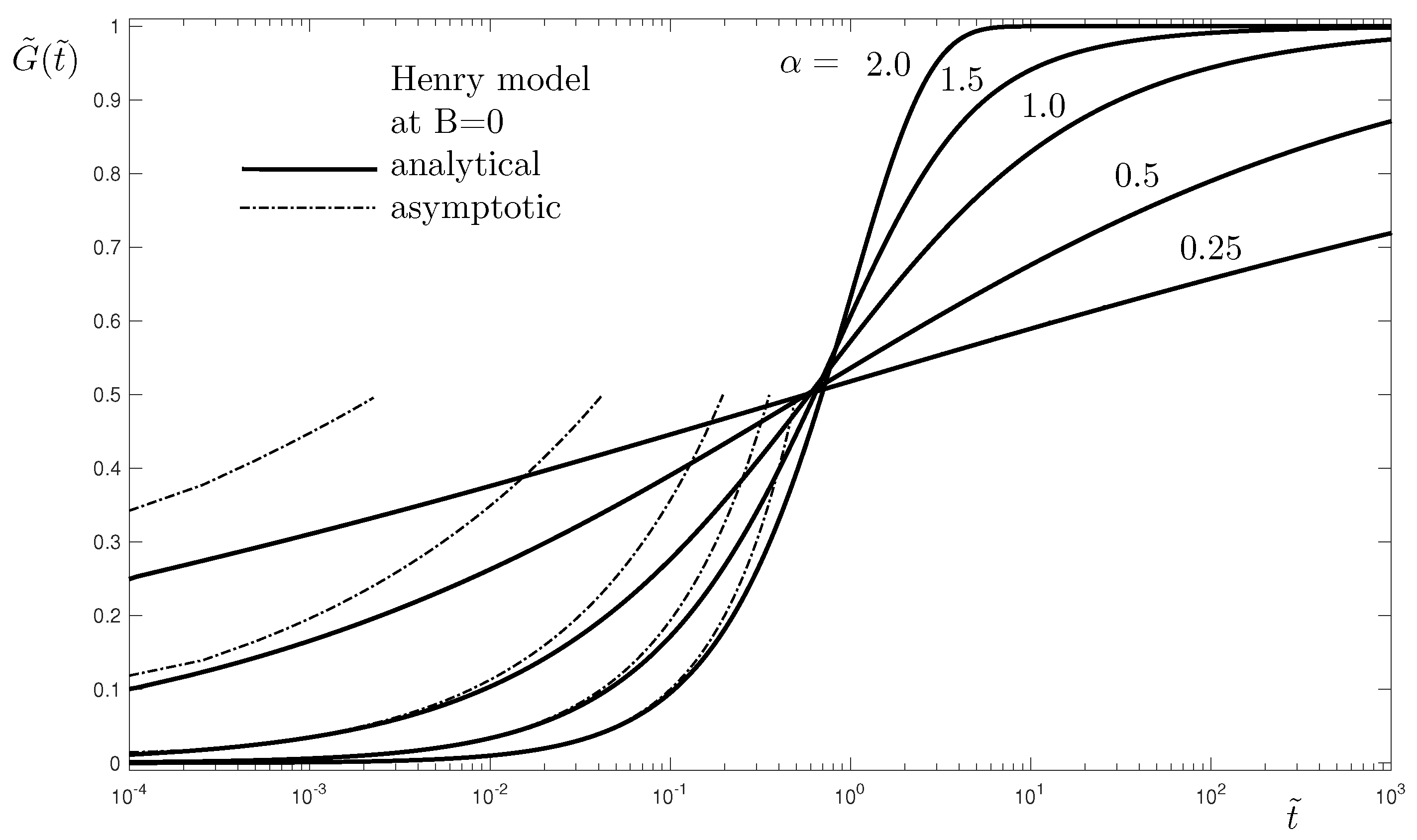Some of them are presented in Figure 3, where very good agreement between the numerical and the analytical results is observed.

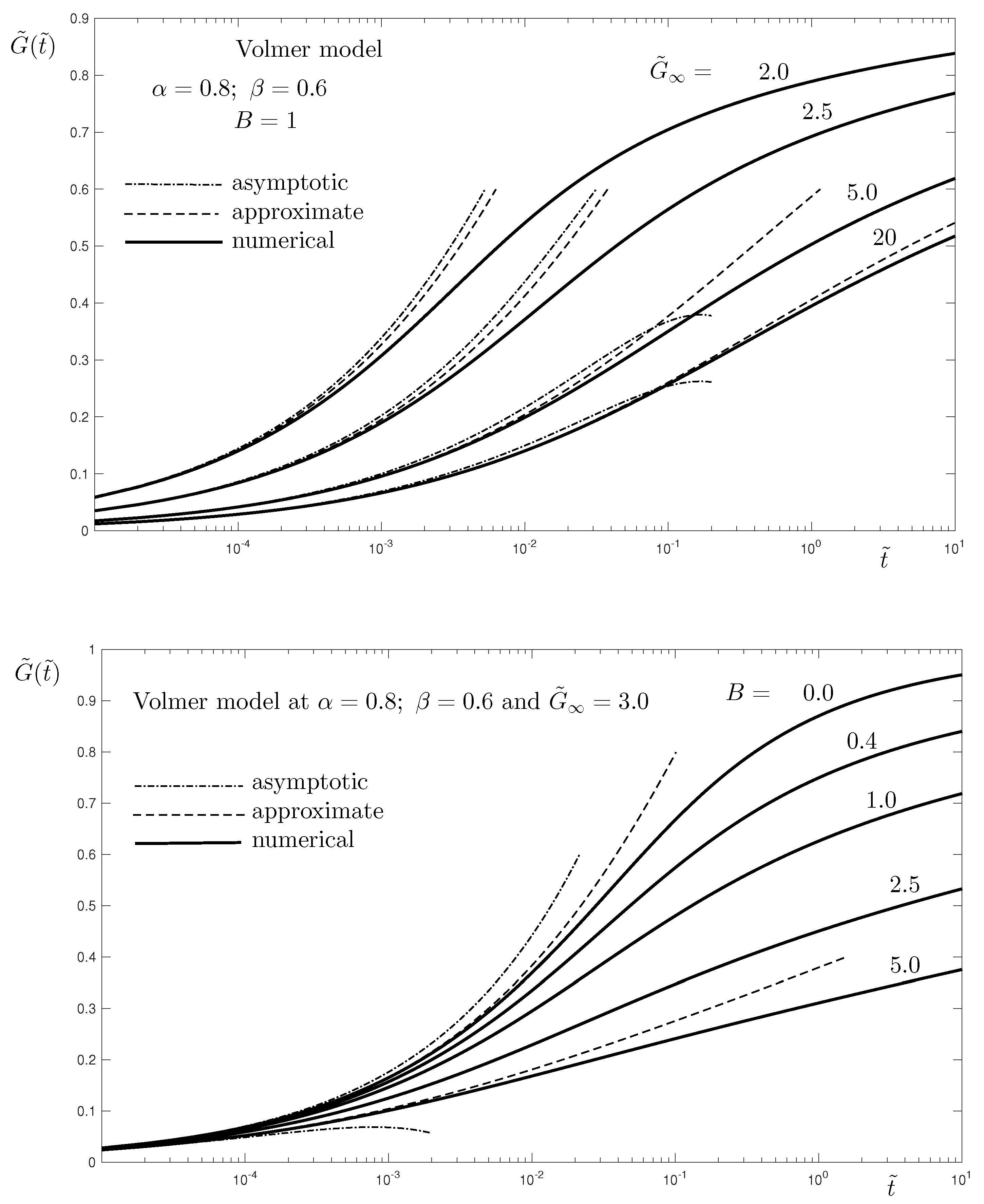
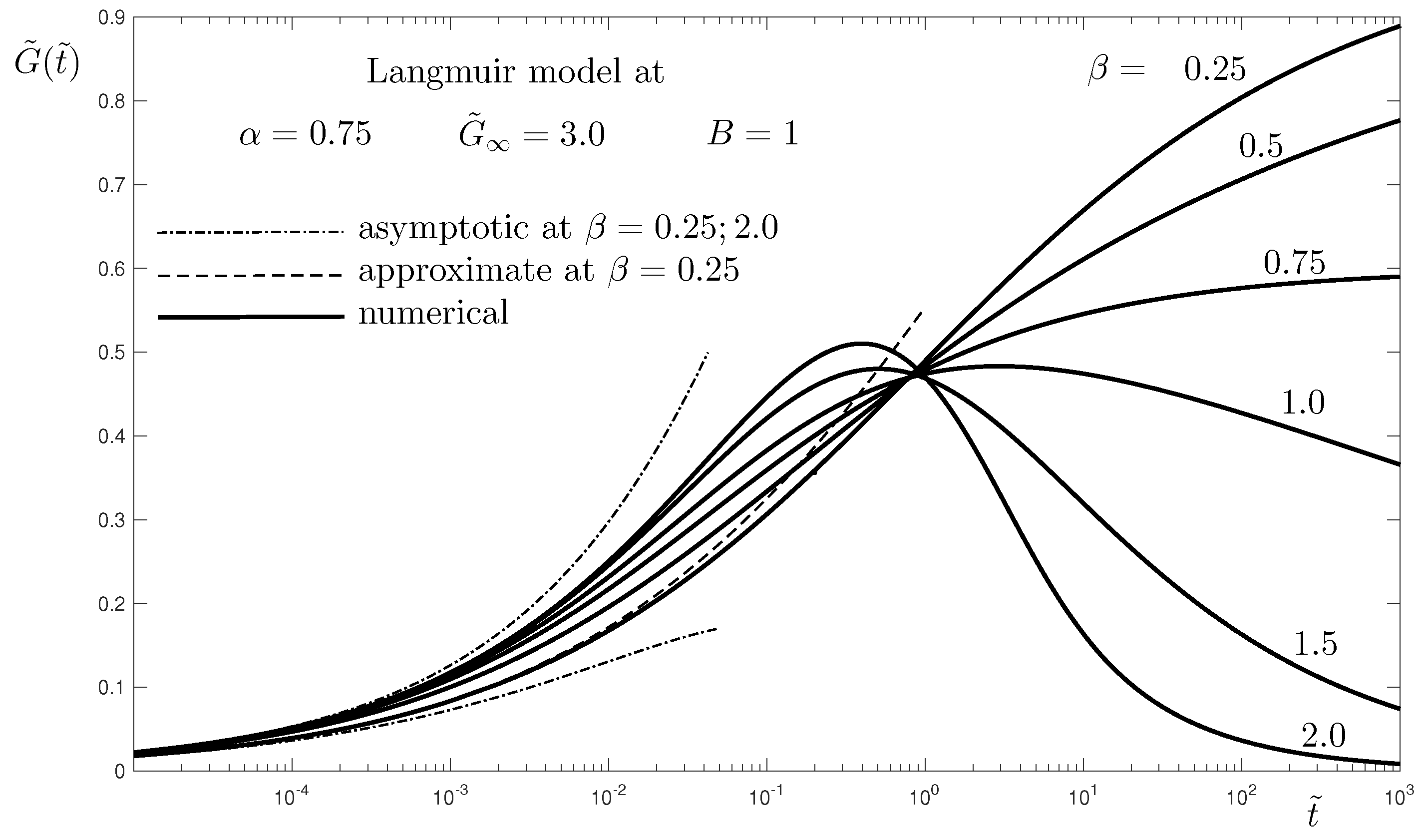
Until the end of this section, results are presented in the case of the nonlinear adsorption isotherms given in Table 1. Figure 4 shows the influence of the parameters ${\tilde{G}}_{\infty }$ (top) and B (bottom) on the evolution of the surfactant concentration. The parameter ${\tilde{G}}_{\infty }=G_{\infty }/G_e$ represents the ratio between the maximum possible surfactant concentration on the interface, $G_{\infty }$, and the equilibrium one, $G_e$. The latter is directly dependent on the surfactant concentration in the bulk $C_e^{+}$, see Equation (26). Thus, an increase of ${\tilde{G}}_{\infty }$ can be considered a decrease of the initially available surfactant in the fluids. This explains the slowdown of the adsorption and, respectively, the desorption, with the increase of ${\tilde{G}}_{\infty }$. The other parameter, B, represents the relative influence of the desorption in the total adsorption–desorption process. This is seen from the governing Equation (27), where the two fractional order terms correspond to the adsorption ($\alpha$ term) and the desorption ($\beta$ term), respectively. Thus, a larger value of B means faster desorption, which explains the results in Figure 4 (bottom); $B=0$ corresponds to the case without desorption, i.e., surfactant is soluble only in Phase 1. This is achieved by setting $d_{\beta }^{-}=0$, when the flux interface-Phase 2 (desorption) is absent, $J^{-}=0$.

Figure 4 shows that the asymptotes (47) at small $\tilde{t}$, derived for the linear case of the Henry isotherm, are also applicable for the other models with nonlinear isotherms, see Table 1. This is due to the fact that the Henry isotherm appears to be an approximation of the nonlinear isotherms. This explains why the asymptotes of the Henry model at $\tilde{t}\to 0$ are also asymptotes for the other models. To investigate this further, let us consider the relation between the Henry isotherm and the other isotherms in their transformed forms $\tilde{f}\left(\tilde{G}\right)$. Using Taylor expansion of $\tilde{f}$, it is easy to see that the adsorption isotherms considered here can be written as:

$$\tilde{f}\left(\tilde{G}\right)=\tilde{G}+O\left({\tilde{G}}^2\right)/{\tilde{G}}_{\infty },$$

(56)

which means that the Henry adsorption isotherm $\tilde{f}\left(\tilde{G}\right)=\tilde{G}$ is a second-order approximation of the Volmer and Langmuir ones at small $\tilde{G}$.

Thus, we can approximate the nonlinear model (27) replacing $\tilde{f}\left(\tilde{G}\right)$ with ${\tilde{G}}_a$ and get:

$${{\tilde{G}}^{\prime }}_a\left(\tilde{t}\right)+D_{\tilde{t}}^{1-\alpha /2}{\tilde{G}}_a\left(\tilde{t}\right)+B{D}_{\tilde{t}}^{1-\beta /2}{\tilde{G}}_a\left(\tilde{t}\right)=\tilde{f}\left(1\right){\displaystyle \frac{{\tilde{t}}^{\alpha /2-1}}{\Gamma (\alpha /2)}}.$$

(57)

The difference between (57) and the governing equation in the case of the linear Henry model (51) is in the coefficient $\tilde{f}\left(1\right)$ on the right-hand side. It is easy to see that the solution ${\tilde{G}}_a$ of the approximating Equation (57) can be presented via the solution of the Henry model:

$${\tilde{G}}_a\left(\tilde{t}\right)=\tilde{f}\left(1\right){\tilde{G}}_H\left(\tilde{t}\right),$$

(58)

where ${\tilde{G}}_H\left(\tilde{t}\right)$ denotes the solution of (51), for which analytical solutions are derived in the previous section. Note that the extra parameter is $\tilde{f}\left(1\right)=f\left(G_e\right){\tilde{G}}_{\infty }$, and the error of the approximation (56) is inversely proportional to ${\tilde{G}}_{\infty }$. That explains why the approximate solution is better at higher values of ${\tilde{G}}_{\infty }$, which is seen in Figure 4 (top).

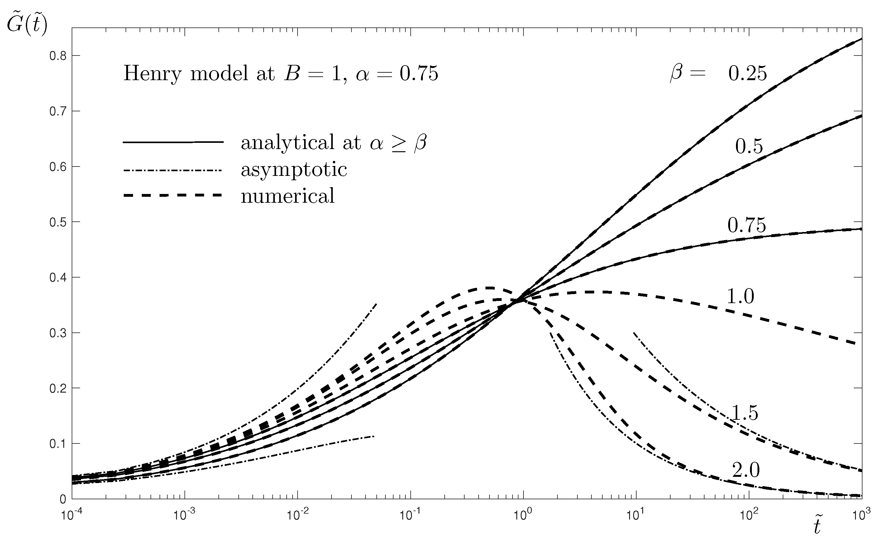
The last results presented here are similar to those given in the linear case, see Figure 3. They are presented in Figure 5, where the fractional order $\beta$ in Phase 2 is varied at given values of the other parameters. As discussed regarding the results in the linear case, there is a transition from increasing surfactant concentration at $\alpha \ge \beta$ to more complex behavior at $\alpha <\beta$. At $\alpha <\beta$, the adsorption at smaller fractional order $\alpha$ is faster for small times $(\tilde{t}<1)$, see Figure 2. At higher $\tilde{t}>1$, the desorption at higher fractional order $\beta$ takes over, leading to a decrease of $\tilde{G}\left(\tilde{t}\right)$. The asymptotic and approximate solutions are presented for $\beta =0.25$. A much more accurate prediction of the approximate solution (dashed line) is observed.

6. Discussion and Conclusions

A time-fractional mathematical model of anomalous diffusion in combination with surfactant adsorption–desorption on/from an interface is studied in the case when the surfactant is soluble in both phases. This model is considered one-dimensional with a flat interface between two semi-infinite phases. This infinite-phase approach adequately describes most physically important situations that involve adsorption dynamics, as discussed in [35]. Since the length scale (thickness of the layer at the interface), where adsorption takes place, is much smaller than the typical size of the particles, the approximation of the flat interface is used. The approach presented in this study can be extended to the cases of finite phases and/or spherical interfaces, which are practically interesting.

Applying the Laplace transform technique, an ordinary multi-term fractional differential equation for the surfactant concentration on the interface is derived. The main contribution of the study is the fractional calculus approach to the problem. Using this approach, an analytical solution in the case of the linear adsorption isotherm is obtained, and asymptotes for small and large times are derived. It is shown that the asymptotes are also applicable in the cases of nonlinear adsorption isotherms.

By the proper rescaling of the concentration and time, the governing equation is transformed into a dimensionless one with a smaller number of parameters. A second-order approximation for a small surfactant concentration, which predicts the dynamics of the process at the beginning, is derived. Using the fractional calculus technique, an integral equation containing two fractional integrals is derived, and a predictor–corrector numerical procedure is developed for its numerical solution. It is used for numerical simulations and investigating the influence of the parameters on the adsorption–desorption process. Both sub- and super-diffusion regimes are covered, where the fractional orders are in the interval $0<\alpha ,\beta \le 2$.

The developed fractional calculus approach could be used for further investigations of other practically interesting regimes of adsorption, for instance, mixed barrier diffusion control.