Abstract
To discuss the fractional order heat conduction based on Youssef’s model, a new mathematical model of a thermoelastic annular cylinder with variable thermal conductivity will be constructed in this work. The Moore–Gibson– Thompson theorem of generalized thermoelasticity will be considered and the governing equations will be derived in dimensionless forms. The Laplace transform technique will be used for a one-dimensional thermoelastic, isotropic, and homogeneous annular cylinder in which the interior surrounded surface is thermally shocked and there is an axial traction-free environment, while the outer surrounded surface has neither heat increment nor cubical deformation. The numerical results will be computed for the Laplace transform inversions by using Tzou’s iteration approach. The distributions of the cubical deformation, invariant average stress, axial stress, and temperature increment will be represented in figures to analyze and discuss. The results show that the fractional-order and variable thermal conductivity parameters have significant effects on all the studied functions. The physical behaviour of the thermal conductivity is closely aligned with the classification of thermal conductivity into weak, normal, and strong categories, which is essential.
1. Introduction
In the history of thermoelasticity theorems, there are five basic theorems that have given us many applications and many improvements in the behaviour of thermoelastic materials. The first theorem is known as uncoupled thermoelasticity, in which mechanical disturbance does not affect the thermal behaviour and the heat conduction equation depends on the classical Fourier law of heat conduction, which is a parabolic differential equation with a nonlimited speed of the thermal wave. Therefore, Biot proposed coupled thermoelasticity (CTE), in which the thermal and mechanical disturbance have mutual influence; however, the heat conduction equation is still a parabolic differential equation, which generates an infinite speed for the thermal wave [1,2,3,4]. Lord and Shulman (L-S) suggested the non-classical Fourier law of heat conduction due to the relaxation time parameter of the heat flux. This parameter makes the heat conduction law depend on a hyperbolic differential equation in which the thermal wave propagates with a finite speed. Therefore, the Lord–Shulman theorem is the first generalization of thermoelasticity theorems [5,6,7,8]. The fourth and fifth theorem of thermoelasticity came from Green and Naghdi (G-N) in [9,10,11,12] and Green and Lindsay (G-L) [3,13,14,15]. Many models and applications in the context of the above theories have been constructed and solved [16,17,18,19,20], and many other applications have been cited [21,22,23,24]. Many models and applications in the context of the above theories have been constructed and solved The theory of Moore–Gibson–Thompson (MGT) is the most recent generalization of thermoelasticity and it has had significant attention in recent years, with several articles dedicated to its research and comprehension, originating from fluid mechanics [25,26,27,28,29,30,31,32]. Youssef introduced a different formula for the law of heat conduction based on the definition of the Riemann–Liouville fractional integral operator [4,33,34,35], and many mathematical models and applications have been studied and discussed in the context of this model [4,20,34,36,37]. Regarding the variability of thermal conductivity as a function of temperature, Godfrey found that many materials such as silicon nitride exhibited a decrease in thermal conductivities of up to 45% for the range of [1–400] degrees Celsius. Therefore, it is important to study and understand how these alterations impact the distributions of the temperature, stress, strain, and displacement in thermoelastic materials [4,38].
Thus, this study introduces a new mathematical model in the context of the Moore–Gibson–Thompson theorem of thermoelasticity based on the fractional-order heat conduction model which has been developed by Youssef. Youssef classified the variability of thermal conductivity into three types: weak conductivity, normal conductivity, and strong conductivity. So, the main goal of this study is to discuss those three types of thermal conductivity for a thermoelastic annular cylinder and to highlight the effect of the fractional-order parameter on the three types of thermal conductivity. Another goal of this work is to compare the current work with traditional works in which the thermal conductivity is constant and there is no fractional heat conduction, to know what new results and contributions this work has made to the study of the behaviour of thermoelastic materials.
The first step is deriving the governing differential equations and applying the Laplace transform techniques to a one-dimensional isotropic, thermoelastic, and homogeneous annular cylinder. The second step is considering the boundary and initial conditions in which the inner surface of the cylinder is exposed to a thermal shock, and there is no axial traction. The third step is using the iteration approach developed by Tzou to compute the numerical Laplace transform inversions. The fourth step is representing the numerical results in graphs for the distributions of temperature increment, cubical strain, axial stress, and invariant average stress, which have been displayed in the figures. The sixth step is constructing the discussions according to the figures of the results. The last step is constructing the conclusions of the results.
2. Basic Formulations
The governing differential equations of an isotropic, thermoelastic, and homogeneous material have been constructed in the context of the Moore–Gibson–Thompson theory of thermoelasticity. The fractional-order heat conduction equation based on Youssef’s model has been considered without either heat sources or external body forces, as follows [17,39]:
The motion equations:
the constitutive stress–strain relations:
where the strain-displacement relations are as below:
In Equations (1)–(3), the temperature increment is given by , gives the reference temperature, the components of the displacement vector are , gives the density, are Lame’s constants (elastic parameters), denotes the Kronecker delta function, and . Moreover, we have , where gives the coefficient of linear thermal expansion.
The fractional heat conduction of Moore–Gibson–Thompson (MGT) with variable thermal conductivity is given in the following form [4,25,26]:
where is the thermal relaxation time or the lag time of heat flux.
The definition of the integral operator is due to the Riemann–Liouville fractional integral operator and it has been taken in a convolution-type form, as is given in [24,25,26]:
The parameter of the fractional-order has an interval to show the case of weak thermal conductivity, and it has an interval to show the case of strong thermal conductivity, while it has the value for usual thermal conductivity.
We have the two variable coefficients and , which define the thermal conductivity and the rate of the thermal conductivity, respectively, as functions of the temperature increment. The parameter defines the specific heat at a constant strain. The function is the cubical dilatation function or the volumetric deformation.
The below relation will be considered in the heat conduction equation as in [4]:
where is known as the relaxation time or the lag time parameter due to temperature gradient.
Hence, we obtain the fractional-order heat conduction equation based on Youssef’s model based on the Moore–Gibson–Thompson theory, as follows:
The specific heat and thermal conductivity relation is satisfied as follows [4,40]:
where denotes the diffusivity of the thermoelastic material.
Hence, we obtain [35] the following:
The following mapping will be applied [4,19,39]:
where denotes the rate of the thermal conductivity at room temperature, which satisfies the following relation:
and gives the usual thermal conductivity at room temperature.
By differentiating Equation (10) with respect to the coordinates, we obtain
By differentiating with respect to the coordinates again, we obtain
By differentiating Equation (10) from the time, we obtain
which gives the following:
Hence, we have the following:
We consider thermal conductivity as a function of the temperature increment by the following linear function [4]:
where is the thermal conductivity parameter that may take a positive or negative value due to the material properties.
Substituting from Equation (17) into the mapping (10) gives
and
Substituting in Equation (1), we obtain
For linearization, the very small nonlinear term will be neglected. Then, we have [4] the following:
3. The Problem Formulation
The region is filled with an isotropic, homogeneous, thermoelastic annular cylindrical material. The coordinate system of the cylinder will be used, in which the z-axis gives the axis of the annular cylinder, as in Figure 1.
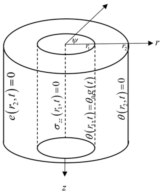
Figure 1.
The thermoelastic, isotropic, homogeneous, and annular cylinder.
Due to the symmetrical shape of the medium, the governing differential equations will be induced in one-dimensional forms. Moreover, all the studied functions will depend on the time “t” and dimensions “r”.
Thus, the components of displacement are , the cubical strain , stress components , and the temperature increment , which gives the governing equations in the forms described below [41,42,43,44,45,46,47,48,49,50].
The equation of motion has the following form [44,45,46,48]:
This equation could be modified to be in the following form:
The fractional-order heat conduction equation has the form [44,45,46,48]:
where .
Heat conduction in the circumferential direction has been disregarded due to the geometric symmetry of the medium about the z-axis.
The constitutive equations are specified in the below forms [44,45,46,48]:
and
The cubical deformation function is given by the following equation:
To obtain simple formulations, the following dimensionless variables will be used [41,43,44,45]:
where and .
The primes will be suppressed for more simplicity.
Hence, Equations (22)–(27) will be in the following forms:
where .
When the value of the fractional-order parameter , we obtain the traditional model.
Laplace transform will be applied as follows:
The Laplace transform of the Riemann–Liouville fractional integral is as follows [33,34]:
The initial conditions are as follows:
Thus, Equations (31)–(35) will be in the following forms:
and
From Equations (41)–(43), we have the invariant average stress as follows:
Equations (39) and (40) take the following forms:
and
where .
By inserting Equation (47) in Equation (46), we obtain
Finally, we obtain the following coupled ordinary differential equations
and
where .
By eliminating the function from Equations (49) and (50), we obtain the following equations:
where and .
Thus, the general solutions of Equation (51) are
and
where the functions and are the modified Bessel functions of the first and second kind of an order of zero, respectively. are parameters and must be determined, and gives the roots of the following characteristic equation:
The inner surface of the cylinder will be loaded by a thermal shock and traction-free in the axial stress direction as follows:
where defines the Heaviside unit-step function which leads to a thermal shock, and is constant.
Then, from Equation (18), we obtain
By using Laplace transform on the above boundary condition, we obtain
Moreover, we have
To use the boundary condition (58) after using the Laplace transform, we must use Equations (43) and (55), which give the following:
where .
The outer surface has no temperature increment, and zero cubical deformation, as follows:
and
Then, after using the Laplace transform, we obtain the following:
and
Applying the boundary conditions, we obtain the following:
By obtaining the solutions of the above system, we have the following:
After obtaining , the original temperature increment could be obtained by solving Equation (18) as follows [4,19]:
Hence, the solutions in the domain of the Laplace transformation are now complete.
The computational analysis of temperature increment, strain, axial stress, and invariant average stress will be carried out using Riemann-sum approximation methods by using the Tzou iteration method as follows [51]:
where “”, “Re” means the real part of any complex function, and “J” is an integer parameter.
For very fast solution convergence, the value “” satisfies the relation [51], and through the computational procedure, we chose the parameter “J” to satisfy the following condition:
4. Numerical Results and Discussion
We will obtain the numerical results and visually illustrate them to discuss the effects of the fractional-order parameter and variability of thermal conductivity on the mechanical and thermal functions.
The copper material has been chosen and, taking into account the subsequent physical constants, the problem constants were established as follows [17,19]:
Due to the above values of parameters, the material has the following dimensionless values [43,44,45]:
We will compute the numerical results for the studied functions within a wide range of dimensionless radial distances for dimensionless time .
The first group of Figure 2, Figure 3, Figure 4 and Figure 5 represents the temperature increment, cubical deformation, axial stress, and invariant average stress distributions with variance values of the fractional order parameter , where gives the state of weak thermal conductivity, gives the state of the normal thermal conductivity, and gives the state of strong thermal conductivity when . The effect of these on the studied functions is shown in the following:
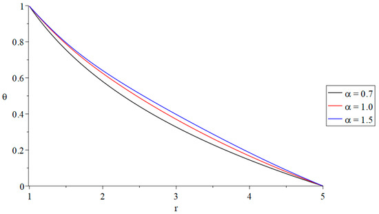
Figure 2.
The temperature increment distributions with variance values of the fractional-order parameter and .
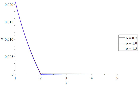
Figure 3.
The cubical deformation distributions with variance values of the fractional-order parameter and .

Figure 4.
The axial stress component distributions with variance values of the fractional-order parameter and .
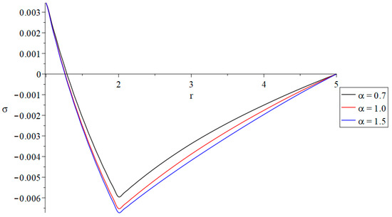
Figure 5.
The invariant average stress distributions with variance values of the fractional-order parameter and .
In Figure 2, the fractional-order parameter has a significant effect on the distribution of the temperature increment. We can see that an increase in the fractional-order parameter leads to an increase in the temperature increment distribution. In other words, the value of the temperature increment in the state of strong thermal conductivity is larger than its values in the state of normal thermal conductivity and than those in the state of weak thermal conductivity. Moreover, the boundary conditions have been satisfied in Figure 2, where the value of the temperature increment in the inner surface of the annular cylinder agrees with the value of the thermal shock , and its value is zero at the outer surface of the annular cylinder .
In Figure 3, the fractional-order parameter has a tiny effect on the distribution of the cubical deformation. Moreover, the boundary conditions have been satisfied in Figure 3 where the value of the cubical deformation in the inner surface of the annular cylinder agrees with the value of the cubical deformation , and its value is zero at the outer surface of the annular cylinder .
In Figure 4, the fractional-order parameter has a significant impact on the distribution of the axial stress component . It is noted that an increase in the fractional-order parameter leads to an increase in the absolute value of the axial stress component distribution. In other words, the value of the axial stress component through the state of strong thermal conductivity is larger than its values in the state of normal thermal conductivity, and larger than those values in the state of weak thermal conductivity. Moreover, the boundary conditions have been satisfied in Figure 4 where the value of the axial stress component in the inner surface of the annular cylinder is zero .
In Figure 5, the fractional order parameter has a significant impact on the distribution of the invariant average stress . It is noted that an increase in the fractional-order parameter leads to an increase in the absolute value of the invariant average stress distribution. This means that the value of the invariant average stress in the state of strong thermal conductivity is larger than its values in the state of normal thermal conductivity and than in the state of weak thermal conductivity.
The second group of Figure 6, Figure 7, Figure 8 and Figure 9 represents the temperature increment, cubical deformation, axial stress, and invariant average stress distributions, with variance values of the thermal conductivity parameter and variance values of the fractional-order parameter when , where gives the state of decreeing thermal conductivity during heating, gives the state of the constant thermal conductivity during heating, and gives the state of increasing thermal conductivity during heating when . The effect on all the studied functions are shown below:
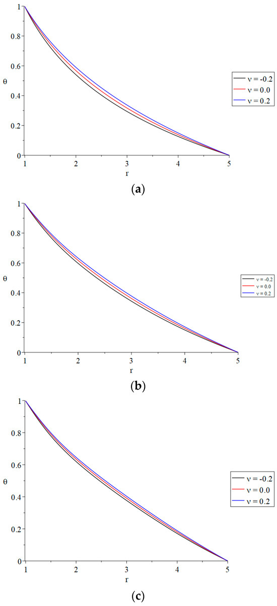
Figure 6.
The temperature increment distributions with variance values of the thermal conductivity parameter and fractional-order parameter. (a): The temperature increment distributions with variance values of the thermal conductivity parameter when (weak thermal conductivity). (b): The temperature increment distributions with variance values of the thermal conductivity parameter when (usual thermal conductivity). (c): The temperature increment distributions with variance values of the thermal conductivity parameter when (strong thermal conductivity).
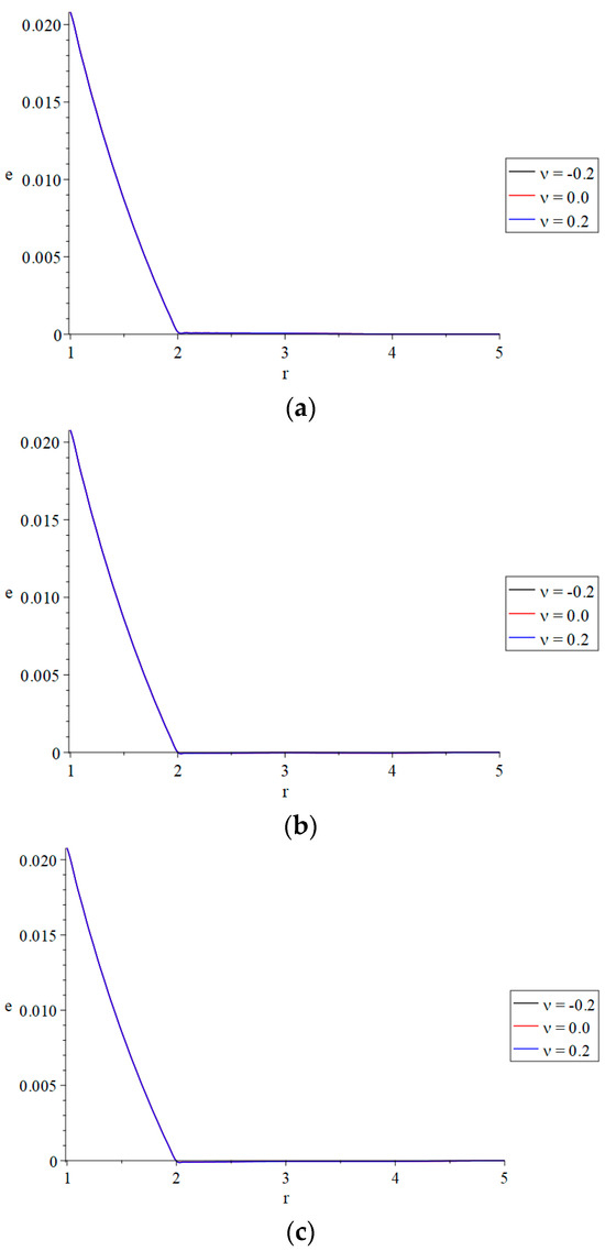
Figure 7.
The cubical deformation distributions with variance values of thermal conductivity parameter and fractional-order parameter. (a): The cubical deformation distributions with variance values of the thermal conductivity parameter when (weak thermal conductivity). (b): The cubical deformation distributions with variance values of the thermal conductivity parameter when (usual thermal conductivity). (c): The cubical deformation distributions with variance values of the thermal conductivity parameter when (strong thermal conductivity).
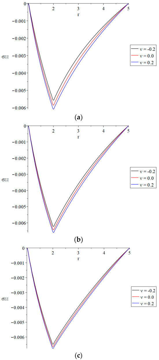
Figure 8.
The axial stress distributions with variance values of the thermal conductivity parameter and the fractional-order parameter. (a): The axial stress distributions with variance values of the thermal conductivity parameter when (weak thermal conductivity). (b): The axial stress distributions with variance values of the thermal conductivity parameter when (usual thermal conductivity). (c): The axial stress distributions with variance values of the thermal conductivity parameter when (strong thermal conductivity).
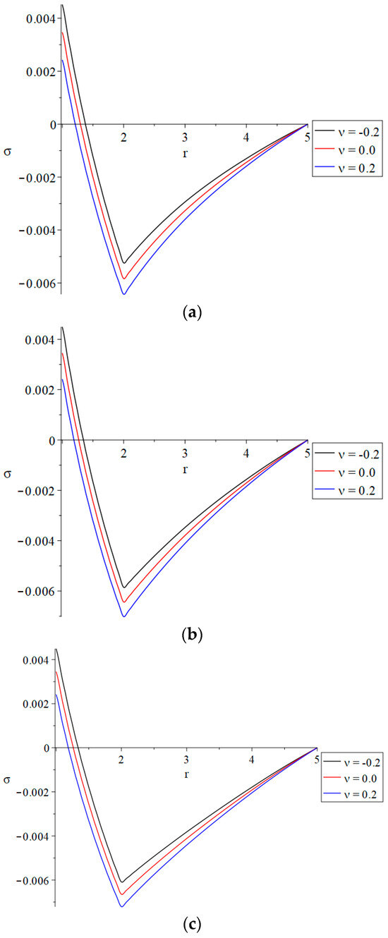
Figure 9.
The invariant average stress distributions with variance values of the thermal conductivity parameter and fractional-order parameter. (a): The invariant average stress distributions with variance values of the thermal conductivity parameter when (weak thermal conductivity). (b): The invariant average stress distributions with variance values of the thermal conductivity parameter when (usual thermal conductivity). (c): The invariant average stress distributions with variance values of the thermal conductivity parameter when (strong thermal conductivity).
In Figure 6a–c, the thermal conductivity parameter has a significant effect on the distribution of the temperature increment. We can see that an increase in the thermal conductivity parameter leads to an increase in the temperature increment distribution. Moreover, increasing the value of the fractional-order parameter leads to decreasing the differences between the value of the temperature increment. This means that, in the strong thermal conductivity case, the values of the temperature increment for the three values of the thermal conductivity parameter are closer to each other than in the usual thermal conductivity case, and closer than in the weak thermal conductivity case.
In Figure 7a–c, the thermal conductivity parameter has a tiny effect on the distribution of the cubical deformation and the fractional-order parameter. The variation in the fractional-order parameter does not make any change in the differences between the three cases of the thermal conductivity for the cubical deformation.
In Figure 8, the thermal conductivity parameter has a significant impact on the distribution of the axial stress component . It is noted that an increase in the thermal conductivity parameter leads to an increase in the absolute value of the axial stress component distribution. Moreover, increasing the value of the fractional-order parameter leads to decreasing the differences between the value of the axial stress component. This means that, in the strong thermal conductivity case, the values of the axial stress component for the three values of the thermal conductivity parameter are closer to each other than in the usual thermal conductivity case, and than in the weak thermal conductivity case.
In Figure 9, the thermal conductivity parameter has a significant impact on the distribution of the invariant average stress . It is noted that an increase in the thermal conductivity parameter leads to an increase in the absolute value of the invariant average stress distribution. The variation in the fractional-order parameter does not make any change in the differences between the three cases of thermal conductivity for the invariant average stress.
5. Conclusions and Future Work
In this work, a mathematical model of an annular thermoelastic cylinder with variable thermal conductivity is presented. Youssef defines the model as fractional-order heat conduction, which is based on the Moore–Gibso–Thompson theorem of thermoelasticity. The governing equations have been applied to a one-dimensional thermoelastic, isotropic, and homogeneous annular cylinder using Laplace transform techniques. The cylinder’s interior surface is subjected to a thermal shock in an axial traction-free environment. The Laplace transform inversions have been numerically computed using Tzou’s iteration procedure. From the numerical results, one can conclude the following:
- •
- The distributions of the temperature increment and stress components are significantly impacted by the fractional-order parameter, which has a considerable impact.
- •
- When the fractional-order parameter is increased, the temperature increment and stress component distributions also rise. This is because of the relationship between the two.
- •
- The values of the temperature increment and the absolute values of the stress components for the state of strong thermal conductivity are greater than their values in the state of normal thermal conductivity and than those in the state of weak thermal conductivity. This is because weak thermal conductivity has a lower thermal conductivity than strong thermal conductivity.
- •
- The distribution of the cubical deformation is not significantly affected by the fractional-order parameter in any way.
- •
- The thermal conductivity parameter has a significant influence on the distribution of the temperature rise as well as the stress components. When the thermal conductivity parameter is increased, the absolute value of the stress components and temperature increment distributions also rise. This is because the thermal conductivity parameter is increased.
- •
- In the strong thermal conductivity case, the values of the temperature increment and axial stress component for the three cases of thermal conductivity are closer to each other than in the usual thermal conductivity case and than in the weak thermal conductivity case.
- •
- The variation in the fractional-order parameter does not make any change in the differences between the three cases of thermal conductivity for the invariant average stress and the cubical deformation.
- •
- While the heat conductivity parameter does have some influence on the distribution of the cubical deformation, it is not very significant.
6. Future Work
In future, the same model could be applied to different bodies such as solid cylinders, solid and annular spheres, and plates.
Funding
This research received no external funding.
Data Availability Statement
Data are contained within the article.
Conflicts of Interest
The author declares that this work has no conflicts of interest.
Nomenclature
| The specific heat without deformation | |
| The speed of the longitudinal wave | |
| Hyperbolic two-temperature parameter | |
| The cubical deformation | |
| Diffusivity | |
| Thermal conductivity | |
| Thermal conductivity at room temperature | |
| The rate of the thermal conductivity | |
| The rate of the thermal conductivity at room temperature | |
| The thermal conductivity parameter | |
| Temperature | |
| Reference temperature | |
| Time | |
| Thermal relaxation time | |
| Lag-time of the temperature gradient | |
| The radius | |
| The displacement function | |
| The z-axis | |
| The linear thermal expansion coefficient | |
| = | |
| The mechanical coupling’s coefficient | |
| The thermoelastic coupling’s coefficient | |
| The coefficient of the thermal viscosity | |
| Lamé’s parameters | |
| The stress tensor | |
| The density |
References
- Biot, M.A. Thermoelasticity and irreversible thermodynamics. J. Appl. Phys. 1956, 27, 240–253. [Google Scholar] [CrossRef]
- Sherief, H.; Naim Anwar, M.; Abd El-Latief, A.; Fayik, M.; Tawfik, A. A fully coupled system of generalized thermoelastic theory for semiconductor medium. Sci. Rep. 2024, 14, 13876. [Google Scholar] [CrossRef] [PubMed]
- Svanadze, M. On the coupled theory of thermoelastic double-porosity materials. J. Therm. Stress. 2022, 45, 576–596. [Google Scholar] [CrossRef]
- Youssef, H.M. Stat-Space Approach to Three-Dimensional Thermoelastic Half-Space Based on Fractional Order Heat Conduction and Variable Thermal Conductivity Under Moor–Gibson–Thompson Theorem. Fractal Fract. 2025, 9, 145. [Google Scholar] [CrossRef]
- Lord, H.W.; Shulman, Y. A generalized dynamical theory of thermoelasticity. J. Mech. Phys. Solids 1967, 15, 299–309. [Google Scholar] [CrossRef]
- Alihemmati, J.; Beni, Y.T. Generalized thermoelasticity of microstructures: Lord-Shulman theory with modified strain gradient theory. Mech. Mater. 2022, 172, 104412. [Google Scholar] [CrossRef]
- Hou, W.; Fu, L.-Y.; Carcione, J.M.; Wang, Z.; Wei, J. Simulation of thermoelastic waves based on the Lord-Shulman theory. Geophysics 2021, 86, T155–T164. [Google Scholar] [CrossRef]
- Bouslimi, J.; Omri, M.; Kilany, A.; Abo-Dahab, S.; Hatem, A. Mathematical model on a photothermal and voids in a semiconductor medium in the context of Lord-Shulman theory. Waves Random Complex Media 2024, 34, 5594–5611. [Google Scholar] [CrossRef]
- Green, A.; Naghdi, P. On undamped heat waves in an elastic solid. J. Therm. Stress. 1992, 15, 253–264. [Google Scholar] [CrossRef]
- Green, A.; Naghdi, P. Thermoelasticity without energy dissipation. J. Elast. 1993, 31, 189–208. [Google Scholar] [CrossRef]
- Hendy, M.M.; Ezzat, M.A. A modified Green-Naghdi fractional order model for analyzing thermoelectric MHD. Int. J. Numer. Methods Heat Fluid Flow 2024, 34, 2376–2398. [Google Scholar] [CrossRef]
- Jagtap, A.D.; Mitsotakis, D.; Karniadakis, G.E. Deep learning of inverse water waves problems using multi-fidelity data: Application to Serre–Green–Naghdi equations. Ocean Eng. 2022, 248, 110775. [Google Scholar] [CrossRef]
- Green, A.; Lindsay, K. Thermoelasticity. J. Elast. 1972, 2, 1–7. [Google Scholar] [CrossRef]
- Sharifi, H. Dynamic response of an orthotropic hollow cylinder under thermal shock based on Green–Lindsay theory. Thin-Walled Struct. 2023, 182, 110221. [Google Scholar] [CrossRef]
- Karimipour Dehkordi, M.; Kiani, Y. Lord–Shulman and Green–Lindsay-based magneto-thermoelasticity of hollow cylinder. Acta Mech. 2024, 235, 51–72. [Google Scholar] [CrossRef]
- Danyluk, M.; Geubelle, P.; Hilton, H. Two-dimensional dynamic and three-dimensional fracture in viscoelastic materials. Int. J. Solids Struct. 1998, 35, 3831–3853. [Google Scholar] [CrossRef]
- Ezzat, M.A.; Youssef, H.M. Three-dimensional thermal shock problem of generalized thermoelastic half-space. Appl. Math. Model. 2010, 34, 3608–3622. [Google Scholar] [CrossRef]
- Ezzat, M.A.; Youssef, H.M. Three-dimensional thermo-viscoelastic material. Mech. Adv. Mater. Struct. 2016, 23, 108–116. [Google Scholar] [CrossRef]
- Youssef, H.; Abbas, I. Thermal shock problem of generalized thermoelasticity for an infinitely long annular cylinder with variable thermal conductivity. Comput. Methods Sci. Technol. 2007, 13, 95–100. [Google Scholar] [CrossRef]
- Youssef, H.M. Two-dimensional thermal shock problem of fractional order generalized thermoelasticity. Acta Mech. 2012, 223, 1219–1231. [Google Scholar] [CrossRef]
- Hafed, Z.S.; Zenkour, A.M. Refined generalized theory for thermoelastic waves in a hollow sphere due to maintained constant temperature and radial stress. Case Stud. Therm. Eng. 2025, 68, 105905. [Google Scholar] [CrossRef]
- Khader, S.; Marrouf, A.; Khedr, M. A model for elastic half space under a visco-elastic layer in generalized thermoelasticity. Contin. Mech. Thermodyn. 2025, 37, 25. [Google Scholar] [CrossRef]
- Yahya, A.; Saidi, A. Response of Generalized Thermoelastic for Free Vibration of a Solid Cylinder with Voids Under a Dual-Phase Lag Model. Iran. J. Sci. Technol. Trans. Mech. Eng. 2025, 1–11. [Google Scholar] [CrossRef]
- Li, S.; Sun, J.; Zhu, J. Analytical solution of dual-phase-lagging generalized thermoelastic damping in Levinson micro/nano rectangular plates. J. Therm. Stress. 2025, 1–19. [Google Scholar] [CrossRef]
- Quintanilla, R. Moore–Gibson–Thompson thermoelasticity. Math. Mech. Solids 2019, 24, 4020–4031. [Google Scholar] [CrossRef]
- Quintanilla, R. Moore-Gibson-Thompson thermoelasticity with two temperatures. Appl. Eng. Sci. 2020, 1, 100006. [Google Scholar] [CrossRef]
- Singh, B.; Mukhopadhyay, S. Galerkin-type solution for the Moore–Gibson–Thompson thermoelasticity theory. Acta Mech. 2021, 232, 1273–1283. [Google Scholar] [CrossRef]
- Bazarra, N.; Fernández, J.R.; Quintanilla, R. Analysis of a Moore–Gibson–Thompson thermoelastic problem. J. Comput. Appl. Math. 2021, 382, 113058. [Google Scholar] [CrossRef]
- Fernández Sare, H.D.; Quintanilla, R. Moore Gibson Thompson thermoelastic plates: Comparisons. J. Evol. Equ. 2023, 23, 70. [Google Scholar] [CrossRef]
- Mondal, S.; Srivastava, A.; Mukhopadhyay, S. Thermoelastic wave propagation and reflection in biological tissue under nonlocal elasticity and Moore–Gibson–Thompson heat conduction: Modeling and analysis. Z. Angew. Math. Phys. 2025, 76, 30. [Google Scholar] [CrossRef]
- Kadian, P.; Kumar, S.; Sangwan, M. Influence of initial stress and gravity on fiber-reinforced thermoelastic solid using Moore–Gibson–Thompson generalized theory of thermoelasticity. Multidiscip. Model. Mater. Struct. 2025, 21, 217–238. [Google Scholar] [CrossRef]
- Ahmed, Y.; Zakria, A.; Osman, O.A.A.; Suhail, M.; Rabih, M.N.A. Fractional Moore–Gibson–Thompson Heat Conduction for Vibration Analysis of Non-Local Thermoelastic Micro-Beams on a Viscoelastic Pasternak Foundation. Fractal Fract. 2025, 9, 118. [Google Scholar] [CrossRef]
- Heymans, N.; Podlubny, I. Physical interpretation of initial conditions for fractional differential equations with Riemann-Liouville fractional derivatives. Rheol. Acta 2006, 45, 765–771. [Google Scholar] [CrossRef]
- Meral, F.; Royston, T.; Magin, R. Fractional calculus in viscoelasticity: An experimental study. Commun. Nonlinear Sci. Numer. Simul. 2010, 15, 939–945. [Google Scholar] [CrossRef]
- Youssef, H.M. Theory of fractional order generalized thermoelasticity. J. Heat Transf. 2010, 132, 061301. [Google Scholar] [CrossRef]
- Youssef, H.M. State-space approach to fractional order two-temperature generalized thermoelastic medium subjected to moving heat source. Mech. Adv. Mater. Struct. 2013, 20, 47–60. [Google Scholar] [CrossRef]
- Youssef, H.M.; Al-Lehaibi, E.A. Fractional order generalized thermoelastic half-space subjected to ramp-type heating. Mech. Res. Commun. 2010, 37, 448–452. [Google Scholar] [CrossRef]
- Hasselman, D.P. Thermal Stresses in Severe Environments; Springer Science & Business Media: Berlin/Heidelberg, Germany, 2012. [Google Scholar]
- Hetnarski, R.B.; Eslami, M.R.; Gladwell, G. Thermal Stresses: Advanced Theory and Applications; Springer: Berlin/Heidelberg, Germany, 2009; Volume 158. [Google Scholar]
- Bahar, L.Y.; Hetnarski, R.B. State space afproach to thermoelasticity. J. Therm. Stress. 1978, 1, 135–145. [Google Scholar] [CrossRef]
- Youssef, H.M. Generalized thermoelasticity of an infinite body with a cylindrical cavity and variable material properties. J. Therm. Stress. 2005, 28, 521–532. [Google Scholar] [CrossRef]
- Youssef, H.M. Two-Temperature Generalized Thermoelastic Infinite Medium with Cylindrical Cavity Subjected to Different Types of Thermal Loading. WSEAS Trans. Heat Mass Transf. 2006, 1, 769. [Google Scholar]
- Youssef, H.M. Problem of generalized thermoelastic infinite medium with cylindrical cavity subjected to a ramp-type heating and loading. Arch. Appl. Mech. 2006, 75, 553–565. [Google Scholar] [CrossRef]
- Youssef, H.M. Generalized thermoelastic infinite medium with cylindrical cavity subjected to moving heat source. Mech. Res. Commun. 2009, 36, 487–496. [Google Scholar] [CrossRef]
- Youssef, H.M. Two-temperature generalized thermoelastic infinite medium with cylindrical cavity subjected to moving heat source. Arch. Appl. Mech. 2010, 80, 1213–1224. [Google Scholar] [CrossRef]
- Ezzat, M.A.; Youssef, H.M. Generalized Magneto-Thermoelasticity For An Infinite Perfect Conducting Body with A Cylindrical Cavity. Mater. Phys. Mech. 2013, 18, 156–170. [Google Scholar]
- Ezzat, M.; El-Bary, A. Effects of variable thermal conductivity and fractional order of heat transfer on a perfect conducting infinitely long hollow cylinder. Int. J. Therm. Sci. 2016, 108, 62–69. [Google Scholar] [CrossRef]
- Youssef, H.M. Theory of generalized thermoelasticity with fractional order strain. J. Vib. Control 2016, 22, 3840–3857. [Google Scholar] [CrossRef]
- El-Bary, A.A.; Youssef, H.M.; Nasr, M.A.E. Hyperbolic two-temperature generalized thermoelastic infinite medium with cylindrical cavity subjected to the non-Gaussian laser beam. J. Umm Al-Qura Univ. Eng. Archit. 2022, 13, 62–69. [Google Scholar] [CrossRef]
- Abbas, I.; Saeed, T.; Alhothuali, M. Hyperbolic two-temperature photo-thermal interaction in a semiconductor medium with a cylindrical cavity. Silicon 2021, 13, 1871–1878. [Google Scholar] [CrossRef]
- Tzou, D.Y. A unified field approach for heat conduction from macro-to micro-scales. J. Heat Transf. 1995, 117, 8–16. [Google Scholar] [CrossRef]
Disclaimer/Publisher’s Note: The statements, opinions and data contained in all publications are solely those of the individual author(s) and contributor(s) and not of MDPI and/or the editor(s). MDPI and/or the editor(s) disclaim responsibility for any injury to people or property resulting from any ideas, methods, instructions or products referred to in the content. |
© 2025 by the author. Licensee MDPI, Basel, Switzerland. This article is an open access article distributed under the terms and conditions of the Creative Commons Attribution (CC BY) license (https://creativecommons.org/licenses/by/4.0/).