A Virtual Element Method for a (2+1)-Dimensional Wave Equation with Time-Fractional Dissipation on Polygonal Meshes

Abstract

We propose a novel space-time discretization method for a time-fractional dissipative wave equation. The approach employs a structured framework in which a fully discrete formulation is produced by combining virtual elements for spatial discretization and the Newmark predictor–corrector method for the temporal domain. The virtual element technique is regarded as a generalization of the finite element method for polygonal and polyhedral meshes within the Galerkin approximation framework. To discretize the time-fractional dissipation term, we utilize the Grünwald-Letnikov approximation in conjunction with the predictor–corrector scheme. The existence and uniqueness of the discrete solution are theoretically proved, together with the optimal convergence order achieved and an error analysis associated with the $H^1$-seminorm and the $L^2$-norm. Numerical experiments are presented to support the theoretical findings and demonstrate the effectiveness of the proposed method with both convex and non-convex polygonal meshes.

1. Introduction

Fractional calculus has become an essential mathematical tool for modeling complex physical phenomena characterized by non-local and anomalous behaviors [1]. Its widespread applicability extends across various disciplines, including anomalous diffusion [2], thermodynamic processes [3], control systems, and bio-fluid dynamics. Over the past decade, substantial progress has been made in the numerical treatment of fractional-order models, particularly through Finite Element Methods (FEMs) [4]. These techniques offer significant advantages over traditional finite difference approaches, ensuring improved accuracy and flexibility in handling complex boundary conditions [5].

Among the most notable contributions, Acosta and Borthagaray [6] provided a rigorous analysis of the convergence properties of FEM discretizations and established fundamental regularity results for solutions to fractional Poisson equations. These theoretical developments were further validated through comprehensive computational experiments [7]. Similarly, Ervin and Roop [8] extended FEM applications to fractional advection–dispersion equations, demonstrating their effectiveness in capturing anomalous transport mechanisms present in diverse physical and engineering systems. The equation considered is as follows.

$$\begin{array}{c}\hfill D\left(p{D}_x^{-\beta }+q_x{D}_1^{-\beta }\right)Du+b\left(x\right)Du+c\left(x\right)u=f,\end{array}$$

where D represents the standard first-order spatial derivative, while $D_x^{-\beta }$ and ${}_{x}D_1^{-\beta }$ denote the left and right fractional integral operators, respectively, constrained by $0\le \beta <1$ and $0\le p,q\le 1$ with $p+q=1$.

Further advancements include solutions to fractional diffusion-wave models via FEM [9], as well as the Petrov–Galerkin FEM approach for fractional convection–diffusion problems in heterogeneous media, formulated as follows:

$$\begin{array}{c}\hfill \left\{\begin{array}{c}{D}_x^{\gamma }u+b{u}^{\prime }+qu=f\mathrm{in}\mathsf{\Omega }=[0,1],\hfill \\ u\left(0\right)=u\left(1\right)=0,\hfill \end{array}\right.\end{array}$$

where $f\in L^2\left(\mathsf{\Omega }\right)$ and $D_x^{\gamma }u$ denote the Caputo fractional derivative of order $\gamma \in (3/2,2)$ [10]. A detailed survey of numerical methodologies for fractional-order models can be found in [11], encompassing various approaches and their practical implementations.

Time-fractional dissipative wave equations have played a crucial role in modeling the physical phenomena of complex systems. The reason has been the simulation of the propagation/dissipation in such media with memory, where the dynamics exhibit certain non-standard diffusion characteristics [9]. The earliest analyses of such model problems considered dissipation with order $\gamma =1$ [12]. In [13], the authors employed the $L1$ approach along with the backward Euler convolution quadrature, also referred to as the Grünwald-Letnikov approximation, to study the nonlinear time-fractional diffusion problems. Furthermore, ref. [14] applied the $L1$ method on a graded mesh for time discretization in order to achieve optimal convergence rates using the $L1$-Galerkin finite element method for nonlinear sub-diffusion problems. A fractional Crank–Nicolson–Galerkin finite element methodology for such model equations has recently been explored in [15].

Symbolic computation plays a crucial role in deriving exact and approximate solutions for nonlinear wave equations, enabling deeper insights into wave propagation and dissipative effects [16]. These techniques are used to validate theoretical findings and ensure consistency in the formulation of the time-fractional dissipative wave equations. Symbolic computation facilitates the precise manipulation of mathematical expressions, aiding in the derivation of closed-form solutions and the stability analysis [17,18].

Nonlinearity also plays a pivotal role in wave equations, influencing wave propagation, stability, and dissipation mechanisms. Recent studies have demonstrated that nonlinear effects can substantially influence wave behavior, leading to complex interactions in various physical systems. For instance, ref. [16] presents advanced nonlinear wave propagation mechanisms, contributing a refined mathematical framework for analyzing wave interactions in complex media. Gao explores in [17] bilinear Auto-Bäcklund transformations and similarity reductions in shallow water wave equations, offering insights into nonlinear wave behavior in oceanic fluid dynamics. Furthermore, ref. [18] highlights and examines a (2+1)-dimensional generalized modified dispersive water-wave system for the nonlinear and dispersive long gravity waves in shallow water of uniform depth. These contributions collectively enhance our understanding of nonlinear wave dynamics, paving the way for further advancements in computational and theoretical wave analysis. However, a notable limitation of these studies is that they do not account for time-fractional dissipation in wave equations. Additionally, we present a novel numerical technique that utilizes the arbitrary polygonal discretization of the spatial domain together with the finite elements for temporal discretization.

In this study, we deal with the following time-fractional dissipative wave equation in two-dimensional space, defined as follows:

$$\begin{array}{c}\hfill {\psi }_{tt}(\mathit{x},t)+{\nu }^R{D}_t^{\gamma }\psi (\mathit{x},t)-\mathsf{\Delta }\psi (\mathit{x},t)=g(\mathit{x},t),(\mathit{x},t)\in \mathsf{\Omega }\times (0,T],\end{array}$$

where $\mathsf{\Omega }$ is a bounded polygonal domain in ${\mathbb{R}}^2$ with boundary $\partial \mathsf{\Omega }$, g represents the source term, and ${}^{R}D_t^{\gamma }\psi$ denotes the $\gamma$th order (where $0<\gamma <1$) Riemann–Liouville fractional derivative of $\psi$ with respect to time.

We further introduce a generalized numerical approach known as the Virtual Element Method (VEM) [19,20]. While there have been few numerical investigations on the 2D wave equations with integer order dissipation, we extend VEM here to the model equation involving fractional order dissipation of the Riemann–Liouville type. The reason for employing VEM in the spatial domain is that it is more adaptable to mesh geometries and can handle polytopal elements [21].

The primary objective of this work is to construct a fully discrete scheme using the Newmark predictor–corrector approach supplemented with Grünwald–Letnikov approximation for time integration and VEM for spatial discretization. Subsequently, a thorough theoretical study is conducted for the fully discrete VEM, supported by numerical illustrations provided in later sections. Some of the significant contributions of this study to the field of computational mathematics and numerical analysis are as follows.

• A comprehensive space-time discretization framework is proposed for the analysis of a time-fractional dissipative wave equation. The approach integrates the VEM for spatial discretization and the Newmark predictor–corrector method for solving time integration, providing a robust framework for fractional wave equations.
• The manuscript extends the capabilities of traditional FEM by employing the VEM, which supports polygonal and polyhedral mesh geometries. This generalization enables the handling of both convex and non-convex meshes, enhancing adaptability to complex domains.
• A key contribution is the use of the Grünwald–Letnikov approximation in conjunction with the predictor–corrector scheme for the accurate discretization of the time-fractional dissipation term. This approach ensures a precise representation of memory effects in dissipative media.
• This study rigorously establishes the existence and uniqueness of the discrete solution for the fully discrete solution, ensuring the soundness and reliability of the proposed method.
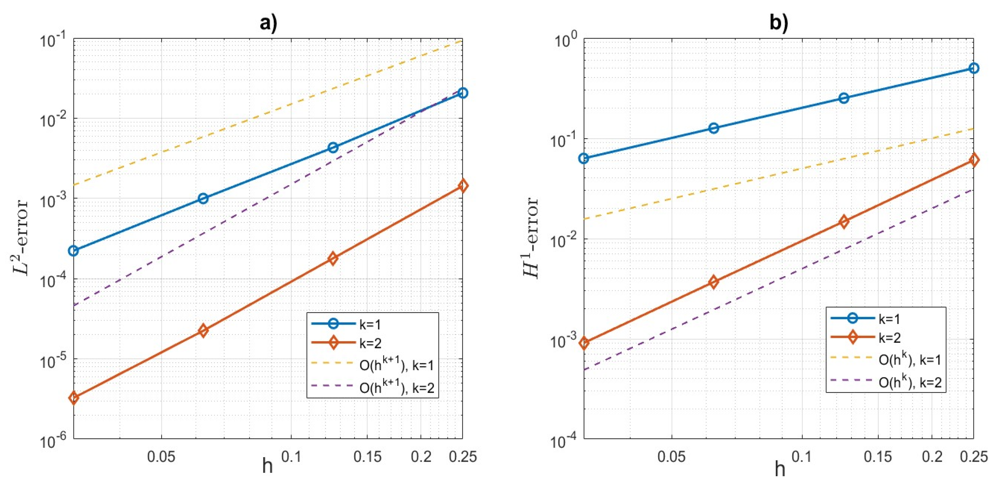
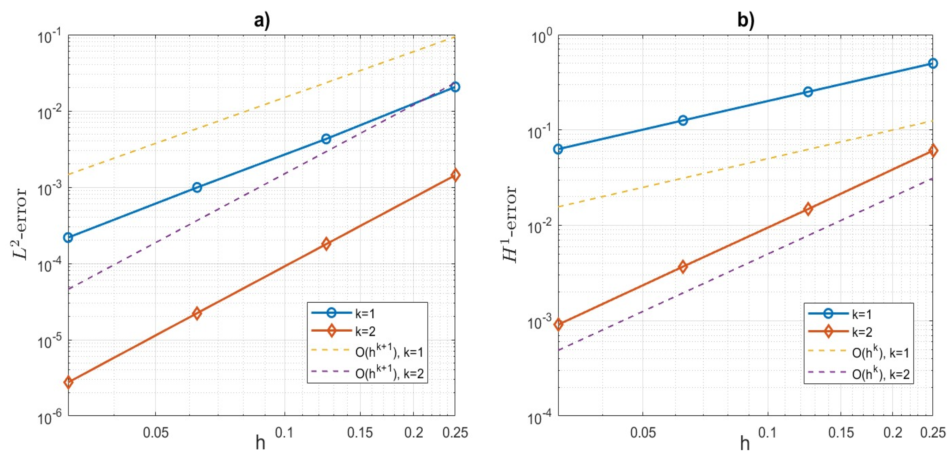
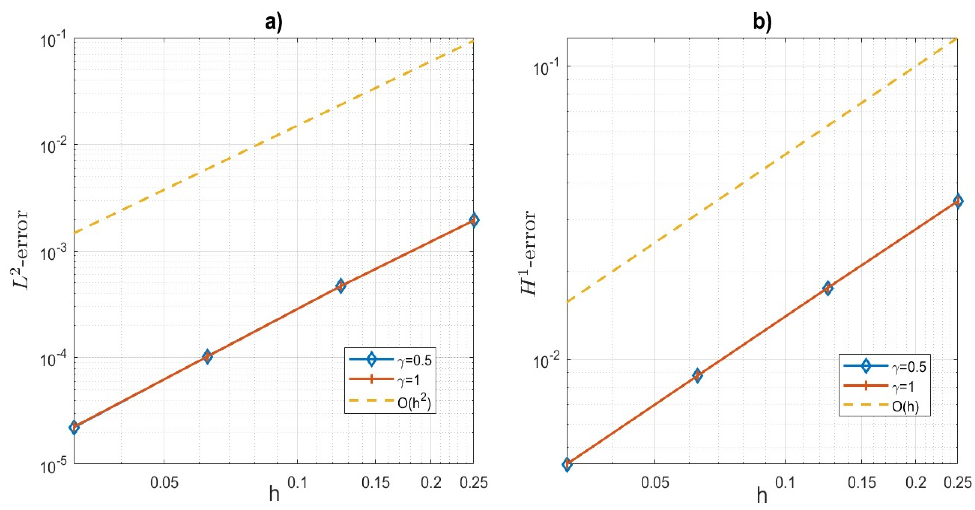
• Optimal convergence rates are achieved and validated through a detailed error analysis in both the $H^1$-seminorm and the $L^2$-norm, confirming the method’s accuracy.
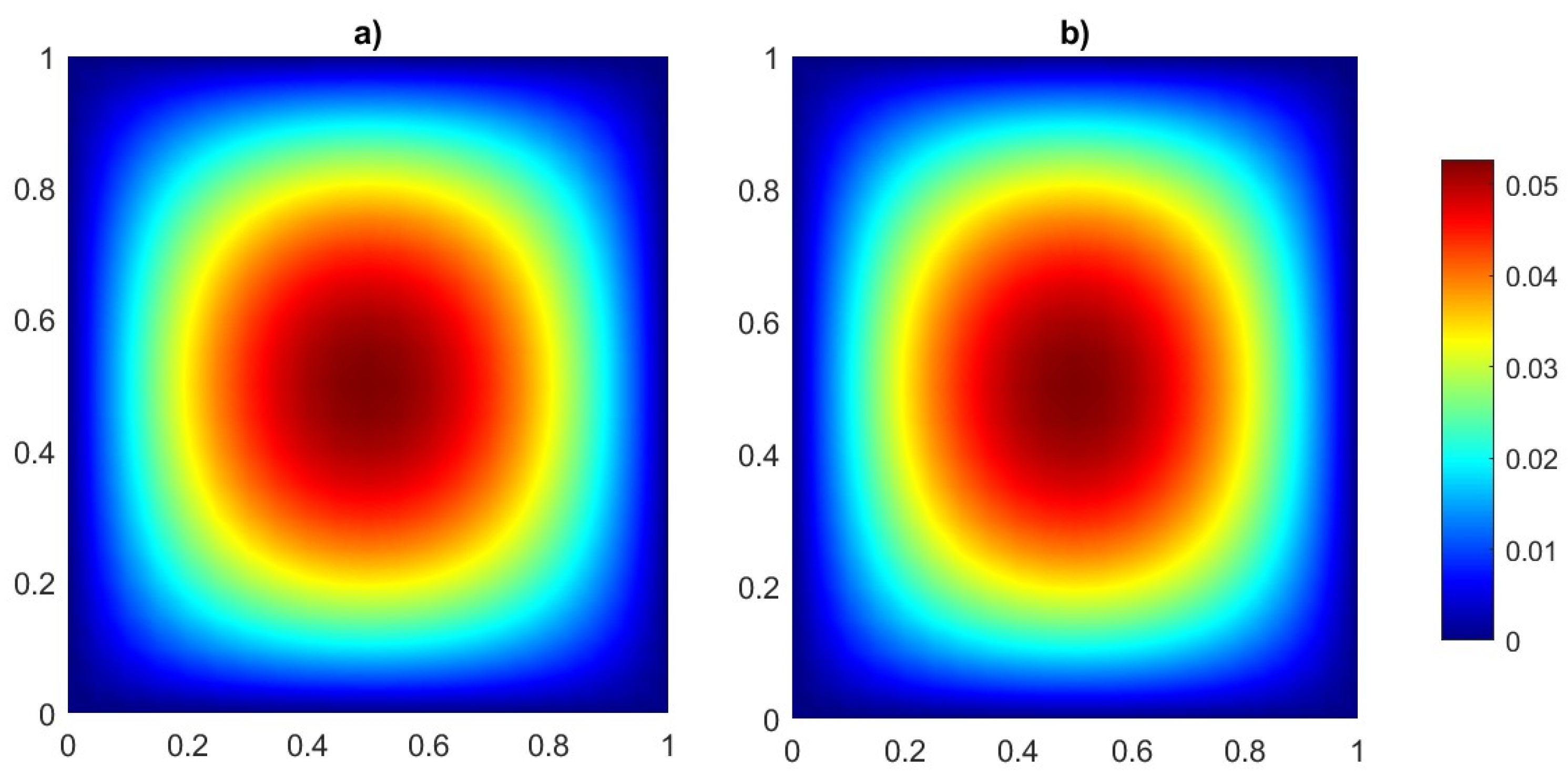
• Extensive numerical experiments are performed on both convex and non-convex polygonal meshes. The results not only validate the theoretical findings but also demonstrate the efficacy of the VEM for arbitrary polygonal discretizations.
• The proposed method provides a computationally efficient and flexible tool for modeling complex physical phenomena, particularly those involving wave propagation and dissipation in media with memory effects.

These contributions collectively advance the state of the art in numerical analysis of time-fractional equations and underscore the versatility and efficiency of the VEM. Our main focus is to lay the foundational mathematical framework of a general time-fractional dissipative wave model, with the construction of a fully discrete scheme, performing a comprehensive theoretical analysis, and validating the method numerically.

Future work will focus on the application of the proposed model to practical problems. Specifically, we aim to study phenomena modeled by generalized dissipative wave equations, with an immediate focus on the subject-specific modeling and mitigation of epileptic seizures.

Outline: The rest of the article is organized as follows. Some early definitions and notation, a mathematical framework of the problem, and important assumptions are described in Section 2, and the continuous problem is presented in Section 3. The main contribution of the study is found in Section 4, in which the fully discrete VEM is derived, presenting a priori estimates, followed by an in-depth error analysis and implementation procedure. Section 5 provides numerical examples that support these theoretical results. Finally, Section 6 concludes the paper with a summary of key findings and future directions.

2. Mathematical Framework

The concept of fractional derivatives has been explored and delineated extensively within the mathematical literature. In this section, we recall the definition of Riemann–Liouville-type fractional derivative, the nonlinear sub-diffusion mathematical model with its variational form.

Definition 1

(Riemann-Liouville fractional derivative). Let $n\in {\mathbb{R}}_{+}$ and $0<\gamma <1$. The operator $D^{n-\gamma }$ is defined by

$$\begin{array}{c}\hfill {}^{R}D^{n-\gamma }\psi \left(t\right):={\displaystyle \frac{1}{\mathsf{\Gamma }\left(\gamma \right)}}{\displaystyle \frac{d^n}{d{t}^n}}{\int }_{s=0}^t{(t-s)}^{\gamma -1}\psi \left(s\right)ds,\end{array}$$

where $\mathsf{\Gamma }(.)$ is the gamma function.

We now describe the mathematical model for the time-fractional dissipative wave equation with a temporal-spatial domain defined as follows: $\mathcal{D}:=\mathsf{\Omega }\times \mathcal{I}\subset {\mathbb{R}}^2\times \mathbb{R}$ with $\mathcal{I}=[0,T]$ and $\partial \mathsf{\Omega }$ representing the boundary of domain $\mathsf{\Omega }$. The model is given by

$$\begin{array}{c}\hfill \left\{\begin{array}{c}{\psi }_{tt}(\mathit{x},t)+{\nu }^R{D}_t^{\gamma }\psi (\mathit{x},t)-\mathsf{\Delta }\psi (\mathit{x},t)=g(\mathit{x},t),(\mathit{x},t)\in \mathcal{D},\hfill \\ \psi (\mathit{x},0)={\varphi }_1\left(\mathit{x}\right),{\psi }_t(\mathit{x},0)={\varphi }_2\left(\mathit{x}\right),\mathit{x}\in \mathsf{\Omega },\hfill \\ \psi (\mathit{x},t)={\psi }_0\left(\mathit{x}\right),\mathit{x}\in \partial \mathsf{\Omega },t\in \mathcal{I},\hfill \end{array}\right.\end{array}$$

(1)

where ${}^{R}D_t^{\gamma }$ is the Riemann–Liouville type fractional derivative of order $\gamma \in (0,1)$, and $\nu$ is a constant dissipative coefficient.

The initial conditions,

$$\begin{array}{c}\hfill \psi (\mathit{x},0)={\varphi }_1,{\psi }_t(\mathit{x},0)={\varphi }_2,\mathit{x}\in \mathsf{\Omega }\end{array}$$

represent the corresponding displacement and velocity at $t=0$. The boundary condition,

$$\begin{array}{c}\hfill \psi (\mathit{x},t)={\psi }_0,(\mathit{x},t)\in \partial \mathsf{\Omega }\times \mathcal{I}\end{array}$$

ensures a prescribed displacement response at the domain boundary, which could correspond to sustained stimulation or a fixed activity level.

To guarantee the existence and uniqueness of a solution to the model problem (1), we introduce the following essential assumption:

Hypothesis 1.

The source term $g(\mathit{x},t)$ belongs to the space $L^2\left(\mathsf{\Omega }\right)$, which implies the following:

$${\parallel g(x,t)\parallel }_{L^2\left(\mathsf{\Omega }\right)}={\left({\int }_{\mathsf{\Omega }}{\left|g(x,t)\right|}^{2}dx\right)}^{1/2}\le C_g,$$

where $C_g$ is a positive constant independent of x and t.

Notations

Throughout this paper, we use the following notations. Let $\mathsf{\Omega }$ be a domain, and let $v\in L^2\left(\mathsf{\Omega }\right)$ denote an arbitrary function. The $L^2$ inner product is given by

$$\langle v,v\rangle ={\int }_{\mathsf{\Omega }}v\left(x\right)v\left(x\right)dx,$$

and the associated $L^2\left(\mathsf{\Omega }\right)$ norm is defined as

$$\parallel v\parallel ={\left({\int }_{\mathsf{\Omega }}{\left|v\left(x\right)\right|}^{2}dx\right)}^{1/2}.$$

For a non-negative integer, n, the Sobolev space $H^n\left(\mathsf{\Omega }\right)$ is defined with the norm

$${\parallel w\parallel }_n={\left(\sum _{0\le s\le n}{∥{\displaystyle \frac{{\partial }^{s}w}{\partial x^s}}∥}^2\right)}^{1/2},$$

and a seminorm, ${\left|w\right|}_n$, which measures the partial derivatives up to order n. The space $C_0^{\infty }\left(\mathsf{\Omega }\right)$ consists of infinitely differentiable functions with compact support in $\mathsf{\Omega }$. Its closure with respect to the norm ${\parallel ·\parallel }_m$ is denoted as $H_0^m\left(\mathsf{\Omega }\right)$. Finally, ${\mathbb{P}}_k\left(\mathsf{\Omega }\right)$ represents the set of all polynomials over $\mathsf{\Omega }$ with the degree at most k.

3. The Continuous Problem

Let us consider the model problem (1) where $\psi$ represents the unknown variable of interest. We assume that the external force $g\in L^2(\mathsf{\Omega }\times (0,T))$ and initial data $\in H_0^1\left(\mathsf{\Omega }\right)$. Then, the standard variational/weak formulation for the model (1) under the Galerkin framework is given as

$$\left\{\begin{array}{c}\mathrm{find}\psi (\mathit{x},t)\in C^0\left(0,T;H_0^1\left(\mathsf{\Omega }\right)\cap C^1(0,T;L^2\left(\mathsf{\Omega }\right)\right)\mathrm{such}\mathrm{that},\hfill \\ m(D_t^2\psi ,w)+m({\nu }^R{D}_t^{\gamma }\psi ,w)+a(\psi ,w)=〈g,w〉\forall w\in H_0^1\left(\mathsf{\Omega }\right)\mathrm{for}\mathrm{a}.\mathrm{e}t\in (0,T),\hfill \\ \psi (\mathit{x},0)={\varphi }_1\left(\mathit{x}\right),{\psi }_t(\mathit{x},0)={\varphi }_2\left(\mathit{x}\right),\mathit{x}\in \mathsf{\Omega },\hfill \end{array}\right.$$

(2)

where the bilinear forms $m(·,·)$ and $a(·,·)$ are defined as

$$\begin{array}{c}\hfill m(\psi ,v)=\underset{\mathsf{\Omega }}{\int }\psi vdx,a(\psi ,v)=\underset{\mathsf{\Omega }}{\int }\nabla \psi ·\nabla vdx,\psi ,v\in H_0^1\left(\mathsf{\Omega }\right),\end{array}$$

and the term $D_t^2\psi$ is intended to be in a weak sense in $(0,T)$. It is well established that the bilinear form $a(·,·)$, also referred to as grad-grad form defined earlier, is continuous and coercive [19], which means that there exists two positive constants (uniform), ${\alpha }_1$ and ${\alpha }_2$, such that

$$\begin{array}{cc}\hfill & a(v,w)\le {\alpha }_1{\left|\right|v\left|\right|}_{H_0^1\left(\mathsf{\Omega }\right)}{\left|\right|w\left|\right|}_{H_0^1\left(\mathsf{\Omega }\right)},\hfill \\ \hfill & a(v,w)\ge {\alpha }_2{\left|\right|w\left|\right|}_{H_0^1\left(\mathsf{\Omega }\right)}^2\forall v,w\in H_0^1\left(\mathsf{\Omega }\right),\hfill \end{array}$$

That simply implies that the weak problem (2) has a unique solution $\psi \left(t\right)$. Also refer to the work of Jin et al. [10,13], in which the well-posedness results of the weak form are proved for time-fractional subdiffusion equations.

4. The Virtual Element Method

The VEM was first introduced for a fundamental Poisson problem in [19], and a guide to the numerical implementation of the higher-order VEM has been addressed [21]. The VEM has a solid mathematical basis, drawing inspiration from the mimetic finite difference method and having characteristics in common with FEM [19]. Over time, VEM has attracted increasing attention in numerical analysis, particularly the problems involving complex domain geometry by facilitating discretization using arbitrary polygonal elements in 2D and polyhedral elements in 3D [21]. The VEM framework has revealed that it serves as a generalization of the FEM over some polygonal and polyhedral meshes. A distinctive aspect of the finite-dimensional VEM space is the presence of non-polynomial functions, which are solutions to certain partial differential equations [20]. These non-polynomial functions are not explicitly known, and therefore, the basis functions of the VEM space are not available in closed form [20].

As is clarified in [21], the explicit definition of the basis functions is not required for computing the mass and stiffness matrices. Instead, suitable polynomial projection operators are defined on the VEM space, and a set of Degrees of Freedom (DoFs) is chosen to ensure the evaluation of the linear and bilinear forms in the discrete scheme. Another key feature of the VEM is its inherent robustness to geometric distortion and its ability to tackle hanging nodes in the meshes. This flexibility makes the VEM a particularly attractive numerical technique to deal with problems involving complex static/evolving domain configurations, frequent mesh adaptations, and high-order solution approximation. Higher-order VEMs have recently received considerable attention. Recent advancements in VEM have demonstrated its applicability to various mathematical models. For instance, conforming and non-conforming VEM approaches have been utilized to solve fourth-order reaction–diffusion equations [22]. Additionally, conservative VEM formulations, both conforming and non-conforming, have been applied to nonlinear Schrödinger models with trapped terms [23]. Zhang et al. contributed significantly by introducing a locally stabilized projection-based VEM designed for higher Reynolds numbers in the context of fractional-order Burgers’ equations [24]. The study is inspired by recent efforts in extending VEM to fractional-order partial differential equations, as explored in [25,26,27,28].

The primary objective of this work is to extend the VEM to a 2D wave equation involving a time-fractional dissipative term. Specifically, we construct a fully discrete VEM scheme using the Euler convolution quadrature supplemented with Grönwall inequality for the temporal direction and VEM for the spatial direction. Subsequently, a comprehensive theoretical study is conducted for the fully discrete VEM, supported with numerical illustrations provided in later sections.

4.1. VEM Discretization

Let ${\mathcal{T}}_h$ be a shape-regularized family of polygons of domain $\mathsf{\Omega }$, with $h_E$ being the diameter of an element $E\in {\mathcal{T}}_h$. Also, let

$$\begin{array}{c}\hfill h:=\underset{E\in {\mathcal{T}}_h}{\max }{h}_E.\end{array}$$

For mesh regularity, we assume the following conditions hold for each element, $E\in {\mathcal{T}}_h$, with some fixed $\rho >0$:

• E is a simply connected polygon with a finite number of straight edges;
• E is star-shaped with respect to a ball of radius at least $\ge \rho h_E$;
• the distance between any two of its vertices is at least $\rho h_E$.

Consider the function space $V_h^E$ over element E, defined in [20] as

$$\begin{array}{c}\hfill V_h^E=\{v_h\in H_0^1\left(E\right):v_h\in C^0(\partial E),\mathsf{\Delta }{v}_h\in {\mathbb{P}}_k\left(E\right),v_h{|}_e\in {\mathbb{P}}_k\left(e\right)\forall \mathrm{edges}e\subset \partial E\}.\end{array}$$

Moreover, define ${\mathsf{\Pi }}_k^{\nabla ,E}:V_h^E\to {\mathbb{P}}_k\left(E\right)$ as the elliptic projection operator, such that

$$\begin{array}{c}\hfill {(\nabla (\psi -{\mathsf{\Pi }}_k^{\nabla ,E}\psi ),\nabla q_k)}_E=0\forall q_k\in {\mathbb{P}}_k\left(E\right)\mathrm{and}{\int }_{\partial E}({\mathsf{\Pi }}_k^{\nabla ,E}\psi -\psi )ds=0,\end{array}$$

and ${\mathsf{\Pi }}_k^{0,E}$, the standard $L^2$-projection onto ${\mathbb{P}}_k\left(E\right)$ defined by

$$\begin{array}{c}\hfill {(\psi -{\mathsf{\Pi }}_k^{0,E}\psi ,q_k)}_E=0\forall q_k\in {\mathbb{P}}_k\left(E\right).\end{array}$$

For each $E\in {\mathcal{T}}_h$, we define the locally “enhanced” virtual element space by utilizing the elliptic projection operator as

$$\begin{array}{c}\hfill W_h^E=\{w_h\in V_h^E:\underset{E}{\int }\left({\mathsf{\Pi }}_k^{\nabla ,E}{w}_h\right)q_{k}dx=\underset{E}{\int }{w}_h{q}_{k}dx\forall q_k\in {\mathbb{P}}_k/{\mathbb{P}}_{k-2}\left(E\right)\},\end{array}$$

where two polynomials are considered equivalent if the degree of their difference does not exceed $k-2$. This equivalence plays a crucial role in defining the virtual element spaces. Specifically, the union of the spaces of homogeneous polynomials of exact degrees k and $k-1$ serves as a key component in the implementation. This structure ensures that the polynomial basis captures the necessary degrees of freedom and maintains consistency within the approximation framework. For polynomial equivalence classes, the quotient space is represented as ${\mathbb{P}}_k/{\mathbb{P}}_{k-2}\left(E\right)$. By assembling the local VEM spaces, the global VEM space is produced and is given as

$$\begin{array}{c}\hfill W_h=\{w\in H_0^1\left(\mathsf{\Omega }\right):w{|}_E\in W_h^E\forall E\in {\mathcal{T}}_h\}.\end{array}$$

Any virtual element function in $w_h\in W_h^E$ is uniquely characterized by the following DoFs (see Figure 1):

• (D1): vertex values $w_h\left(V_i\right)$ for $k\ge 1$, where $V_i$ are the vertices of E;
• (D2): on each edge e of $\partial E$ for $k>1$, the values of $w_h$ at the $(k-1)$ internal Gauss-Lobatto quadrature points;
• (D3): the polynomial moments for $k\ge 2$

  $$\begin{array}{c}\hfill \underset{E}{\int }{v}_h{p}_{k-2}dx\forall p_{k-2}\in {\mathbb{P}}_{k-2}\left(E\right).\end{array}$$

These DoFs are assembled in an $H^1$-conforming manner to define the global VEM space of order k. The unisolvence of these degrees of freedom has been established in [20], ensuring that each virtual element function is uniquely determined by them. An essential characteristic of the local virtual element space is that the projections ${\mathsf{\Pi }}_k^{\nabla ,E}{w}_h$ and ${\mathsf{\Pi }}_k^{0,E}{w}_h$ can be computed directly from the DoFs (D1)–(D2) associated with $w_h\in W_h^E$. These projections play a central role in constructing the discrete formulation and implementing the virtual element method efficiently.

The semi-discrete VEM approximation of the weak formulation (2) can be stated as follows:

Find ${\psi }_h(\mathit{x},t)\in W_h$ for almost every $t\in (0,T)$, such that

$$\begin{array}{c}\hfill \left\{\begin{array}{c}{m}_h(D_t^2{\psi }_h,w_h)+m_h(\nu {}^{R}D_t^{\gamma }{\psi }_h,w_h)+a_h({\psi }_h,w_h)=\langle g_h,w_h\rangle \forall w_h\in W_h,\hfill \\ {\psi }_h(\mathit{x},0)={\varphi }_1\left(\mathit{x}\right),{\psi }_h^{\prime }(\mathit{x},0)={\varphi }_2\left(\mathit{x}\right),\mathit{x}\in \mathsf{\Omega }.\hfill \end{array}\right.\end{array}$$

Here, the global discrete bilinear forms $a_h(·,·):W_h\times W_h\to \mathbb{R}$ and $m_h(·,·):W_h\times W_h\to \mathbb{R}$ are defined as follows:

$$\begin{array}{cc}\hfill & a_h({\psi }_1,{\psi }_2)=\sum _{E\in {\mathcal{T}}_h}{a}_h^E({\psi }_1,{\psi }_2)\forall {\psi }_1,{\psi }_2\in W_h,\hfill \\ \hfill & m_h({\psi }_1,{\psi }_2)=\sum _{E\in {\mathcal{T}}_h}{m}_h^E({\psi }_1,{\psi }_2)\forall {\psi }_1,{\psi }_2\in W_h,\hfill \end{array}$$

where both $a_h^E(·,·):W_h^E\times W_h^E\to \mathbb{R}\mathrm{and}{m}_h^E(·,·):W_h^E\times W_h^E\to \mathbb{R}$ are locally computable, defined as follows:

$$\begin{array}{cc}\hfill & a_h^E({\psi }_{h1},{\psi }_{h2})=a^E({\mathsf{\Pi }}_k^{\nabla ,E}{\psi }_{h1},{\mathsf{\Pi }}_k^{\nabla ,E}{\psi }_{h2})+{\mathcal{S}}_a^E((I-{\mathsf{\Pi }}_k^{\nabla ,E}){\psi }_{h1},(I-{\mathsf{\Pi }}_k^{\nabla ,E}){\psi }_{h2})\forall {\psi }_{h1},{\psi }_{h2}\in W_h^E,\hfill \\ \hfill & m_h^E({\psi }_{h1},{\psi }_{h2})=m^E({\mathsf{\Pi }}_k^{0,E}{\psi }_{h1},{\mathsf{\Pi }}_k^{0,E}{\psi }_{h2})+{\mathcal{S}}_m^E((I-{\mathsf{\Pi }}_k^{0,E}){\psi }_{h1},(I-{\mathsf{\Pi }}_k^{0,E}){\psi }_{h2})\forall {\psi }_{h1},{\psi }_{h2}\in W_h^E,\hfill \end{array}$$

where ${\mathcal{S}}_a^E:W_h^E\times W_h^E\to \mathbb{R}$ and ${\mathcal{S}}_m^E:W_h^E\times W_h^E\to \mathbb{R}$ are symmetric positive–definite stabilizing bilinear forms, satisfying

$$\begin{array}{cc}\hfill & c_0{a}^E(v_h,v_h)\le {\mathcal{S}}_a^E(v_h,v_h)\le c_1{a}^E(v_h,v_h)\forall v_h\in W_h^E,\hfill \\ \hfill & d_0{m}^E(v_h,v_h)\le {\mathcal{S}}_m^E(v_h,v_h)\le d_1{m}^E(v_h,v_h)\forall v_h\in W_h^E,\hfill \end{array}$$

for some positive constants $c_0,c_1,d_0\mathrm{and}{d}_1$ independent of h and E.

The stability of $a_h^E(·,·)$ and $m_h^E(·,·)$ is guaranteed through these stabilization terms (a formal description is given below). This work adopts $computable$ “dofi-dofi” stabilization (see [29]), which is an essential component of the VEM, to ensure numerical stability and consistency on general polygonal meshes. We provide explicit definitions of the stabilization terms ${\mathcal{S}}_a^E$ and ${\mathcal{S}}_m^E$:

• Stabilization for Stiffness Term

The stiffness stabilization term ${\mathcal{S}}_a^E(u,v)$ is defined by

$${\mathcal{S}}_a^E(u,v)=\sum _{i,j=1}^{N_E}{\mathrm{dof}}_i\left(u\right){\mathrm{dof}}_j\left(v\right),$$

where $N_E$ is the number of degrees of freedom for the element, and ${\mathrm{dof}}_i\left(u\right)$ is the value of u at the $i^{th}$ DoF.

• Stabilization for Mass Term:

The mass stabilization term ${\mathcal{S}}_m^E(u,v)$ is defined by

$${\mathcal{S}}_m^E(u,v)=h_E^2\sum _{i,j=1}^{N_E}{\mathrm{dof}}_i\left(u\right){\mathrm{dof}}_j\left(v\right),$$

where $h_E$ is the diameter of the element E.

The bilinear forms $a_h^E(·,·)$ and $m_h^E(·,·)$ possess key properties that ensure the robustness of the method, as stated in the following results.

Proposition 1

(Polynomial Consistency). Given $w_h\in W_h^E$, $\forall E\in {\mathcal{T}}_h$ it holds that

$$\begin{array}{cc}\hfill a_h^E(p,w_h)& =a^E(p,w_h)\forall p\in {\mathbb{P}}_k\left(E\right),\hfill \\ \hfill m_h^E(p,w_h)& =m^E(p,w_h)\forall p\in {\mathbb{P}}_k\left(E\right).\hfill \end{array}$$

Proof. 

The polynomial consistency follows from the definition of locally computable discrete bilinear forms and the use of the fact that ${\mathsf{\Pi }}_k^{\nabla ,E}$ is an identity operator on ${\mathbb{P}}_k\left(E\right)$. Since ${\mathsf{\Pi }}_k^{\nabla ,E}{\mathbb{P}}_k\left(E\right)={\mathbb{P}}_k\left(E\right)$, it follows that

$$\begin{array}{c}\hfill {\mathcal{S}}_a^E(q-{\mathsf{\Pi }}_k^{\nabla ,E}\left(q\right),w_h-{\mathsf{\Pi }}_k^{\nabla ,E}\left(w_h\right))=0\forall q\in {\mathbb{P}}_k\left(E\right),w_h\in W_h^E.\end{array}$$

So, using the definition of ${\mathsf{\Pi }}_k^{\nabla ,E}$, we have

$$\begin{array}{c}\hfill a_h^E(p,w_h)=a^E({\mathsf{\Pi }}_k^{\nabla ,E}\left(p\right),{\mathsf{\Pi }}_k^{\nabla ,E}\left(w_h\right))=a^E(p,{\mathsf{\Pi }}_k^{\nabla ,E}{w}_h)=a^E(p,w_h),\end{array}$$

which proves the polynomial consistency. The second part can be proved similarly.    □

Proposition 2

(Stability). There exist two pairs of constants, $({\alpha }_{*},{\alpha }^{*})$ and $({\beta }_{*},{\beta }^{*})$, both independent of h, with $0<{\alpha }_{*}\le {\alpha }^{*}$ and $0<{\beta }_{*}\le {\beta }^{*}$, such that, for any $w_h\in W_h^E$, the following equivalences hold:

$$\begin{array}{cc}\hfill & {\alpha }_{*}{a}^E(w_h,w_h)\le a_h^E(w_h,w_h)\le {\alpha }^{*}{a}^E(w_h,w_h),\hfill \\ \hfill & {\beta }_{*}{m}^E(w_h,w_h)\le m_h^E(w_h,w_h)\le {\beta }^{*}{m}^E(w_h,w_h).\hfill \end{array}$$

Proof. 

Using the symmetry of bilinear forms and stabilization terms, we have

$$\begin{array}{cc}\hfill a_h^E(w_h,w_h)& \le a^E({\mathsf{\Pi }}_k^{\nabla ,E}\left(w_h\right),{\mathsf{\Pi }}_k^{\nabla ,E}\left(w_h\right))+c_1{a}^E(w_h-{\mathsf{\Pi }}_k^{\nabla ,E}\left(w_h\right),w_h-{\mathsf{\Pi }}_k^{\nabla ,E}\left(w_h\right))\hfill \\ \hfill & \le \max (1,c_1)\left(a^E({\mathsf{\Pi }}_k^{\nabla ,E}\left(w_h\right),{\mathsf{\Pi }}_k^{\nabla ,E}\left(w_h\right))+a^E(w_h-{\mathsf{\Pi }}_k^{\nabla ,E}\left(w_h\right),w_h-{\mathsf{\Pi }}_k^{\nabla ,E}\left(w_h\right))\right)\hfill \\ \hfill & ={\alpha }^{*}{a}^E(w_h,w_h),\hfill \end{array}$$

and

$$\begin{array}{cc}\hfill a_h^E(w_h,w_h)& \ge a^E({\mathsf{\Pi }}_k^{\nabla ,E}\left(w_h\right),{\mathsf{\Pi }}_k^{\nabla ,E}\left(w_h\right))+c_0{a}^E(w_h-{\mathsf{\Pi }}_k^{\nabla ,E}\left(w_h\right),w_h-{\mathsf{\Pi }}_k^{\nabla ,E}\left(w_h\right))\hfill \\ \hfill & \ge \min (1,c_0)\left(a^E({\mathsf{\Pi }}_k^{\nabla ,E}\left(w_h\right),{\mathsf{\Pi }}_k^{\nabla ,E}\left(w_h\right))+a^E(w_h-{\mathsf{\Pi }}_k^{\nabla ,E}\left(w_h\right),w_h-{\mathsf{\Pi }}_k^{\nabla ,E}\left(w_h\right))\right)\hfill \\ \hfill & ={\alpha }_{*}{a}^E(w_h,w_h),\hfill \end{array}$$

which proves the stability of $a_h^E(·,·)$. Similarly, we can prove the stability of $m_h^E(·,·)$.    □

These conditions ensure that the non-polynomial parts ${\mathcal{S}}_a^E(·,·)$ and ${\mathcal{S}}_m^E(·,·)$ scale similarly to the polynomial parts of $a_h^E(·,·)$ and $m_h^E(·,·)$, respectively.

4.2. A Fully Discrete Scheme

The Grünwald-Letnikov approximation and Caputo definition provide general approximations of fractional derivatives achieving consistency orders of 1 and 2, respectively. These methods enable the numerical evaluation of fractional derivatives by transforming them into finite-type sums involving only integer-order derivatives. To construct a fully-discrete scheme, it is necessary to discretize the fractional derivative in the temporal direction. For some K, a positive integer, let $t_0<t_1<\dots <t_K$ be the partition of the interval $[0,T]$ with uniform step-length $\tau$. The Grünwald-Letnikov (GL) formula is used to approximate the Riemann-Liouville (RL) fractional derivative, which is defined as follows:

$$\begin{array}{c}\hfill {}^{R}D_t^{\alpha }u\left(t\right)={\displaystyle \frac{1}{\mathsf{\Gamma }(1-\alpha )}}{\int }_0^t{\displaystyle \frac{u\left(s\right)}{{(t-s)}^{\alpha }}}ds.\end{array}$$

Using the GL scheme, the discrete approximation of the RL derivative at $t_{n+1}=(n+1)\tau$ is given by

$$\begin{array}{c}\hfill {}^{R}D_t^{\alpha }{u}^{n+1}\approx {\displaystyle \frac{1}{{\tau }^{\alpha }}}\sum _{k=0}^{n+1}{w}_k{u}^{n+1-k},\end{array}$$

(3)

where

• $\tau$ is the uniform time step size,
• $u^{n+1}$ represents the numerical solution at the ${(n+1)}^{\mathrm{th}}$ time step,
• $w_k$ are the Grünwald weights computed as follows:

  $$w_k={(-1)}^k{\displaystyle \frac{\mathsf{\Gamma }(\alpha +1)}{\mathsf{\Gamma }(k+1)\mathsf{\Gamma }(\alpha -k+1)}}.$$

The weighted summation over past values ($u^{n+1-k}$) effectively captures the memory effects inherent in fractional dynamics. In [30], the authors present a fully discrete numerical scheme for solving strongly nonlinear time-fractional parabolic problems using the Grünwald–Letnikov method for time discretization and a second-order central difference scheme for spatial discretization. This work establishes sharp error bounds using a Grönwall-type inequality and complementary discrete kernels, ensuring the stability and accuracy of the numerical method wherein well-posedness results are rigorously established, providing confidence in the correctness of the scheme. The results indicate that the proposed scheme achieves first-order temporal convergence away from the initial time, and fractional-order convergence near the initial time. The findings are particularly relevant for modeling complex wave propagation and diffusion processes. We rely on this work to establish the usefulness of the Grünwald–Letnikov approximation for the dissipative term in our model.

Remark 1.

To achieve second-order accuracy, Jin et al. [15] utilized the following approximation to R-L type derivative at point $t=t_{n-{\displaystyle \frac{\gamma }{2}}}$:

$$\begin{array}{c}\hfill {}^{R}D_{\tau }^{\gamma }\psi (\mathit{x},t_n)={}^{R}D_{t_{n-{\displaystyle \frac{\gamma }{2}}}}^{\gamma }\psi (\mathit{x},t)+\mathcal{O}\left({\tau }^2\right),\end{array}$$

where ${}^{R}D_{\tau }^{\gamma }$ is a discrete fractional differential operator. This second-order accuracy result was originally observed by Dimitrov [31], under suitable compatibility conditions and assuming the solution $\psi \in C^3[0,T]$.

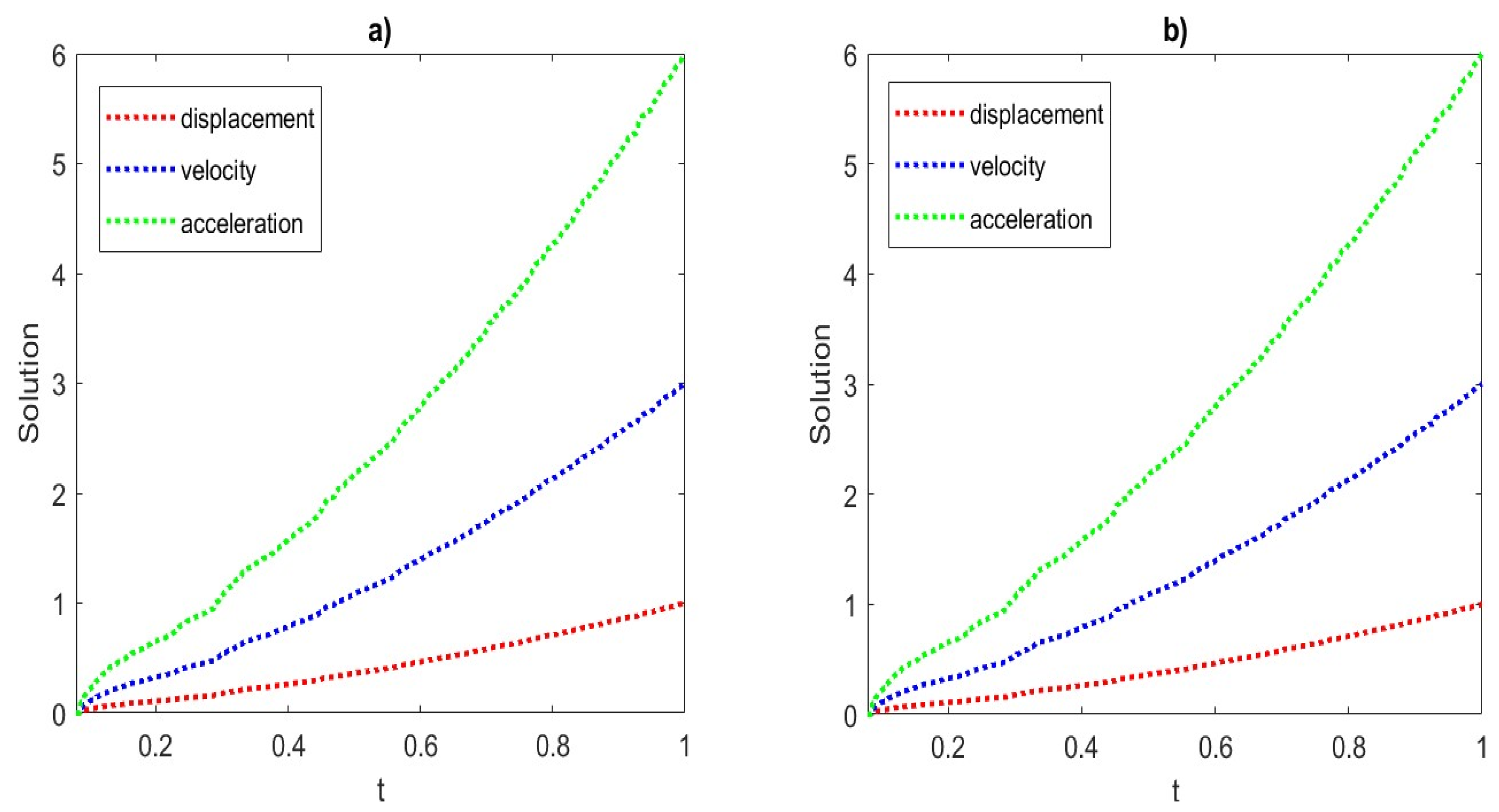
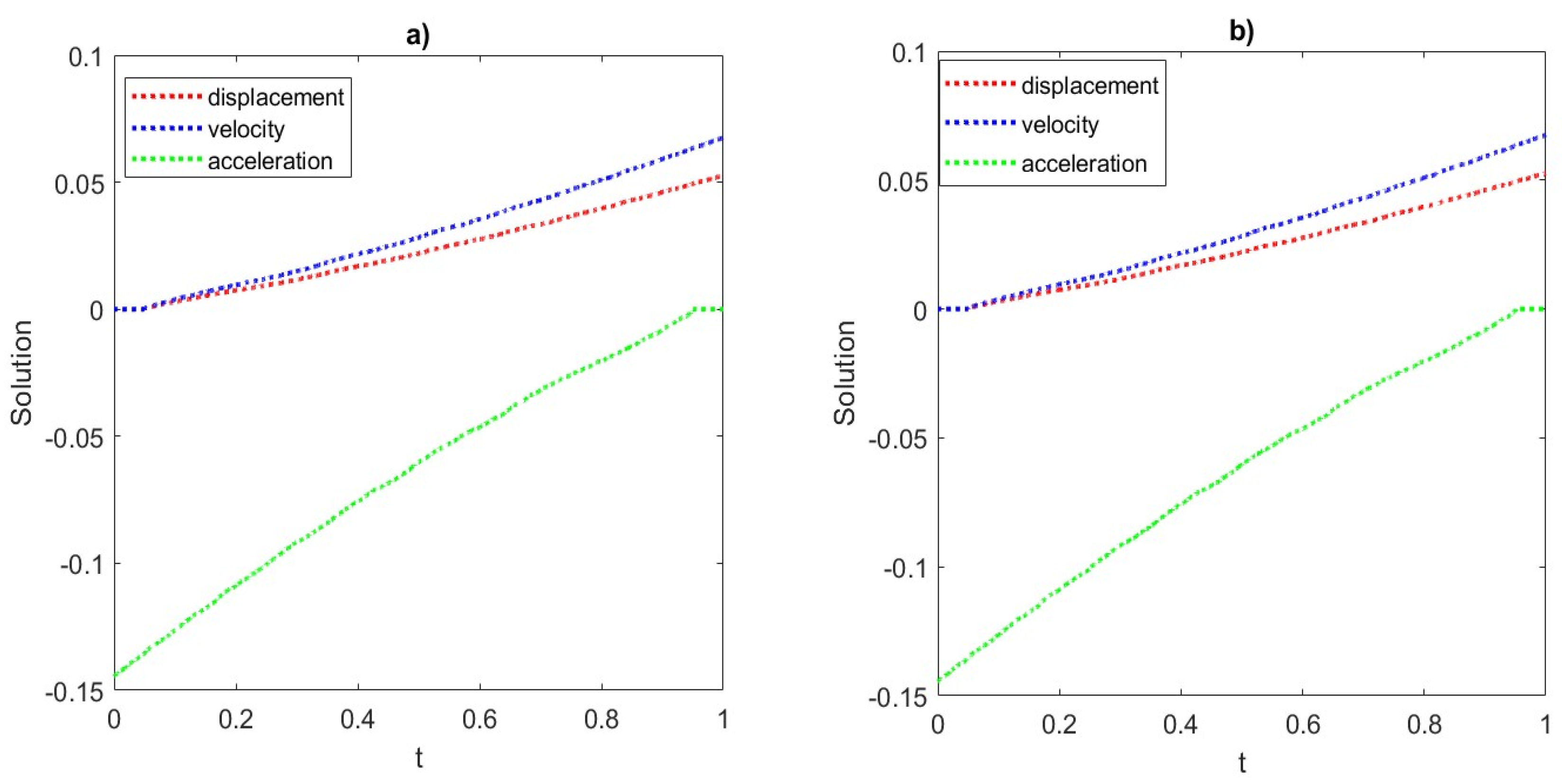
We now construct the approximation in the temporal domain by using the Newmark predictor–corrector method [32] in conjunction with Grünwald–Letnikov approximation (3) for the time-fractional dissipative term. The resultant scheme will be a fully discrete scheme of the model problem (1). Before presenting the fully discrete scheme, we briefly summarize the Newmark approach. Let $\beta$ and $\lambda$ be two Newmark parameters. From the model Equation (1), we assume ${\varphi }_1$ and ${\varphi }_2$ as initial displacement and velocity respectively, with $\mathcal{A}$ representing the acceleration. Assuming ${\mathcal{A}}_0$ to be the initial acceleration, the predictor step yields the following approximations:

$$\begin{array}{cc}\hfill & {\varphi }_{(1,p)}={\varphi }_1+\tau {\varphi }_2+(0.5-\beta ){\tau }^2{\mathcal{A}}_0,\hfill \\ \hfill & {\varphi }_{(2,p)}={\varphi }_2+(1-\lambda )\tau {\mathcal{A}}_0.\hfill \end{array}$$

Solving for the acceleration ${\mathcal{A}}_n$, find ${\mathcal{A}}_h^n\in W_h$, $n=1,2,\dots ,K$, such that

$$\begin{array}{c}\hfill m_h({\mathcal{A}}_h^n,w_h)+m_h({\varphi }_{(2,p)h}^{n,\gamma },w_h)+a_h({\varphi }_{(1,p)h}^n,w_h)=〈g_h,w_h〉-\sum _{j=1}^{n-1}{m}_h({\mathcal{A}}_h^j,w_h)\forall w_h\in W_h.\end{array}$$

Using the corrector step, the updated displacement and velocity are given as follows:

$$\begin{array}{cc}\hfill & {\varphi }_1={\varphi }_{(1,p)}+\beta {\tau }^2{\mathcal{A}}_n,\hfill \\ \hfill & {\varphi }_2={\varphi }_{(2,p)}+\lambda \tau {\mathcal{A}}_n.\hfill \end{array}$$

We recall some important well-known facts associated with Newmark method:

• Convergence: The method achieves at least a convergence rate of $\mathcal{O}\left(\tau \right)$, while the higher accuracy of $\mathcal{O}\left({\tau }^2\right)$ is obtained specifically when $\lambda =1/2$.
• Accuracy: With $\lambda =1/2$ and $\mathcal{O}\left({\tau }^2\right)$ accuracy, is unconditionally stable for $\beta \ge 0.25$. When $\beta <0.25$, the stability condition requires that the time step size $\tau$ satisfy a suitable constraint, as discussed in [32].

Now, using the definition of operator ${}^{R}D_{t_n}^{\gamma }$ from the Equation (3), together with the Newmark predictor–corrector method, we obtain the fully discrete scheme:

$$\begin{array}{cc}\hfill m_h({\mathcal{A}}_h^n,w_h)+{\tau }^{-\gamma }{w}_0^{\left(\gamma \right)}{m}_h({\varphi }_{(2,p)h}^n,w_h)+a_h({\varphi }_{(1,p)h}^n,w_h)=& 〈g_h,v_h〉-\sum _{j=1}^{n-1}{m}_h({\mathcal{A}}_h^j,w_h)\hfill \\ \hfill & -{\tau }^{-\gamma }\sum _{j=1}^{n-1}{w}_{n-j}^{\left(\gamma \right)}{m}_h({\varphi }_{(2,p)h}^j,w_h).\hfill \end{array}$$

(4)

This discrete formulation results in a system of algebraic equations that can be solved to obtain the virtual element approximation.

4.3. Well-Posedness

To establish the existence and uniqueness of solutions for the fully discrete VEM, we rely on a key proposition based on Brouwer’s fixed point theorem is employed [33], stated as follows.

Proposition 3.

Let $\mathcal{H}$ be a finite-dimensional Hilbert space equipped with norm $\parallel ·\parallel$ and inner product $\langle ·,·\rangle$. Suppose $G:\mathcal{H}\to \mathcal{H}$ is a continuous mapping satisfying

$$\langle G\left(w\right),w\rangle >0\forall w\in \mathcal{H},\parallel w\parallel =\rho ,\rho >0.$$

Then, there exists an element, $v\in \mathcal{H}$, such that

$$G\left(v\right)=0\mathit{and}\parallel v\parallel <\rho .$$

Theorem 1

(Wellposedness). Let ${\psi }_h^0,\dots ,{\psi }_h^{n-1}$ be the numerical solutions obtained by solving Equation (4). Then, for any time step $1\le n\le K$, the discrete scheme (4) admits a unique solution ${\psi }_h^n.$

Proof. 

Rewriting Equation (4) as

$$\begin{array}{cc}\hfill m_h({\psi }_h^n,v_h)+{\tau }^{-\gamma }{w}_0^{\left(\gamma \right)}{m}_h({\psi }_h^n,v_h)& +a_h({\psi }_h^n,v_h)-〈g_h,v_h〉+\sum _{j=1}^{n-1}{m}_h({\psi }_h^j,v_h)\hfill \\ \hfill & +{\tau }^{-\gamma }\sum _{j=1}^{n-1}{w}_{n-j}^{\left(\gamma \right)}{m}_h({\psi }_h^j,v_h)=0,\hfill \end{array}$$

(5)

and multiplying Equation (5) by $\left(1-{\displaystyle \frac{\gamma }{2}}\right)$, we get the equivalent form

$$\begin{array}{cc}\hfill & m_h({\psi }_h^n,v_h)+{\tau }^{-\gamma }{w}_0^{\left(\gamma \right)}{m}_h({\psi }_h^n,v_h)+\left(1-{\displaystyle \frac{\gamma }{2}}\right)a_h({\psi }_h^n,v_h)+\left(1-{\displaystyle \frac{\gamma }{2}}\right)\sum _{j=1}^{n-1}{m}_h({\psi }_h^j,v_h)\hfill \\ \hfill & +{\tau }^{-\gamma }\left(1-{\displaystyle \frac{\gamma }{2}}\right)\sum _{j=1}^{n-1}{w}_{n-j}^{\left(\gamma \right)}{m}_h({\psi }_h^j,v_h)-\left(1-{\displaystyle \frac{\gamma }{2}}\right)〈g_h,v_h〉-\left({\displaystyle \frac{\gamma }{2}}\right)m_h({\psi }_h^{n-1},v_h)\hfill \\ \hfill & -{\tau }^{-\gamma }\left({\displaystyle \frac{\gamma }{2}}\right)w_0^{\left(\gamma \right)}{m}_h({\psi }_h^{n-1},v_h)=0.\hfill \end{array}$$

(6)

Now, we define the operator $S:W_h\to W_h$, such that

$$\begin{array}{cc}\hfill m(S\left(X^n\right),U):=& m_h(X^n,U)+{\tau }^{-\gamma }{w}_0^{\left(\gamma \right)}{m}_h(X^n,U)+\left(1-{\displaystyle \frac{\gamma }{2}}\right)a_h(X^n,U)-\left(1-{\displaystyle \frac{\gamma }{2}}\right)〈g_h,U〉\hfill \\ \hfill & +\left(1-{\displaystyle \frac{\gamma }{2}}\right)\sum _{j=1}^{n-1}{m}_h({\psi }_h^j,U)+{\tau }^{-\gamma }\left(1-{\displaystyle \frac{\gamma }{2}}\right)\sum _{j=1}^{n-1}{w}_{n-j}^{\left(\gamma \right)}{m}_h({\psi }_h^j,U)\hfill \\ \hfill & -\left({\displaystyle \frac{\gamma }{2}}\right)m_h({\psi }_h^{n-1},U)-{\tau }^{-\gamma }\left({\displaystyle \frac{\gamma }{2}}\right)w_0^{\left(\gamma \right)}{m}_h({\psi }_h^{n-1},U).\hfill \end{array}$$

(7)

Since S is continuous, we choose $U=X^n$, and obtain

$$\begin{array}{cc}\hfill m(S\left(X^n\right),X^n):=& m_h(X^n,X^n)+{\tau }^{-\gamma }{w}_0^{\left(\gamma \right)}{m}_h(X^n,X^n)+\left(1-{\displaystyle \frac{\gamma }{2}}\right)a_h(X^n,X^n)-\left(1-{\displaystyle \frac{\gamma }{2}}\right)〈g_h,X^n〉\hfill \\ \hfill & +\left(1-{\displaystyle \frac{\gamma }{2}}\right)\sum _{j=1}^{n-1}{m}_h({\psi }_h^j,X^n)+{\tau }^{-\gamma }\left(1-{\displaystyle \frac{\gamma }{2}}\right)\sum _{j=1}^{n-1}{w}_{n-j}^{\left(\gamma \right)}{m}_h({\psi }_h^j,X^n)\hfill \\ \hfill & -\left({\displaystyle \frac{\gamma }{2}}\right)m_h({\psi }_h^{n-1},X^n)-{\tau }^{-\gamma }\left({\displaystyle \frac{\gamma }{2}}\right)w_0^{\left(\gamma \right)}{m}_h({\psi }_h^{n-1},X^n).\hfill \end{array}$$

(8)

Using the projection operator ${\mathsf{\Pi }}_k^{\nabla ,E}$, the bilinear form $a_h(·,·)$ is defined as follows:

$$a_h(U_h^{n,\gamma },v_h)={\int }_{\mathsf{\Omega }}\nabla {\mathsf{\Pi }}_k^{\nabla ,E}{U}_h^{n,\gamma }·\nabla {\mathsf{\Pi }}_k^{\nabla ,E}{v}_{h}dx+s_a^E(U_h^{n,\gamma },v_h),$$

where $s_a^E(·,·)$ is a stabilization term ensuring that $a_h$ is coercive, that is,

$$a_h(U_h^{n,\gamma },U_h^{n,\gamma })\ge C{\parallel U_h^{n,\gamma }\parallel }_{H^1\left(\mathsf{\Omega }\right)}^2,$$

where $C>0$ is a coercivity constant and is independent of the mesh size h. The equivalence of this inequality in $L^2\left(\mathsf{\Omega }\right)$ can be derived using the Poincarè inequality, which relates the $H^1\left(\mathsf{\Omega }\right)$-seminorm to the $L^2\left(\mathsf{\Omega }\right)$-norm:

$$a_h(U_h^{n,\gamma },U_h^{n,\gamma })\ge C{C}_P\parallel U_h^{n,\gamma }{\parallel }_{L^2\left(\mathsf{\Omega }\right)}^2\ge C_a{\parallel U_h^{n,\gamma }\parallel }_{L^2\left(\mathsf{\Omega }\right)}^2 ,$$

where $C_P>0$ is the Poincarè constant dependent on the domain $\mathsf{\Omega }$. Additionally, the mass bilinear form satisfies

$$m_h(U_h^{n,\gamma },U_h^{n,\gamma })\ge C_m{\parallel U_h^{n,\gamma }\parallel }_{L^2\left(\mathsf{\Omega }\right)}^2 ,$$

with $C_m>0$.

From Hypothesis 1, we have the boundedness of the source term g, which satisfies

$$\begin{array}{c}\hfill \left|\right|g\left(X^n\right)\left|\right|\le C_g\left(\right||X^n\left|\right|),C_g>0.\end{array}$$

(9)

Using the Cauchy–Schwarz inequality in the Equation (8), together with inequality (9) and the assumption that $w_j^{\left(\gamma \right)}<0,1\le j\le n$, we have

$$\begin{array}{cc}\hfill m(S\left(X^n\right),X^n)& \ge w_0^{\left(\gamma \right)}\left|\right|X^n{\left|\right|}^2+\left(1-{\displaystyle \frac{\gamma }{2}}\right){\tau }^{\left(\gamma \right)}\left|\right|X^n{\left|\right|}^2+\left(1-{\displaystyle \frac{\gamma }{2}}\right){\tau }^{\left(\gamma \right)}{C}_g\left(\right||X^n\left|\right|\left)\right||X^n\left|\right|\hfill \\ \hfill & +{\tau }^{\left(\gamma \right)}\left(1-{\displaystyle \frac{\gamma }{2}}\right)\sum _{j=1}^{n-1}\left|\right|{\psi }_h^j\left|\right|\left|\right|X^n\left|\right|+\left(1-{\displaystyle \frac{\gamma }{2}}\right)\sum _{j=1}^{n-1}{w}_{n-j}^{\left(\gamma \right)}\left|\right|{\psi }_h^j\left|\right|\left|\right|X^n\left|\right|\hfill \\ \hfill & -{\tau }^{\left(\gamma \right)}\left({\displaystyle \frac{\gamma }{2}}\right)\left|\right|{\psi }_h^{n-1}\left|\right|\left|\right|X^n\left|\right|-\left({\displaystyle \frac{\gamma }{2}}\right)w_0^{\left(\gamma \right)}\left|\right|{\psi }_h^{n-1}\left|\right|\left|\right|X^n\left|\right|.\hfill \end{array}$$

(10)

Since ${\tau }^{\gamma }\left|\right|X^n\left|\right|>0$, Equation (10) can be rewritten as

$$\begin{array}{cc}\hfill m(S\left(X^n\right),X^n)& \ge (\left(w_0^{\left(\gamma \right)}+\left(1-{\displaystyle \frac{\gamma }{2}}\right){\tau }^{\left(\gamma \right)}{C}_g\right)\left|\right|X^n\left|\right|+{\tau }^{\left(\gamma \right)}\left(1-{\displaystyle \frac{\gamma }{2}}\right)\sum _{j=1}^{n-1}\left|\right|{\psi }_h^j\left|\right|\hfill \\ \hfill & -{\tau }^{\left(\gamma \right)}\left({\displaystyle \frac{\gamma }{2}}\right)\left|\right|{\psi }_h^{n-1}\left|\right|+\left(1-{\displaystyle \frac{\gamma }{2}}\right)\sum _{j=1}^{n-1}{w}_{n-j}^{\left(\gamma \right)}\left|\right|{\psi }_h^j\left|\right|-\left({\displaystyle \frac{\gamma }{2}}\right)w_0^{\left(\gamma \right)}\left|\right|{\psi }_h^{n-1}\left|\right|\left)\right||X^n\left|\right|.\hfill \end{array}$$

Thus $m(S\left(X^n\right),X^n)>0$, provided that

$$\begin{array}{cc}\hfill & \left(w_0^{\left(\gamma \right)}+\left(1-{\displaystyle \frac{\gamma }{2}}\right){\tau }^{\left(\gamma \right)}{C}_g\right)\left|\right|X^n\left|\right|+{\tau }^{\left(\gamma \right)}\left(1-{\displaystyle \frac{\gamma }{2}}\right)\sum _{j=1}^{n-1}\left|\right|{\psi }_h^j\left|\right|-{\tau }^{\left(\gamma \right)}\left({\displaystyle \frac{\gamma }{2}}\right)\left|\right|{\psi }_h^{n-1}\left|\right|\hfill \\ \hfill & +\left(1-{\displaystyle \frac{\gamma }{2}}\right)\sum _{j=1}^{n-1}{w}_{n-j}^{\left(\gamma \right)}\left|\right|{\psi }_h^j\left|\right|-\left({\displaystyle \frac{\gamma }{2}}\right)w_0^{\left(\gamma \right)}\left|\right|{\psi }_h^{n-1}\left|\right|>0.\hfill \end{array}$$

By choosing ${\tau }^{\gamma }<{\displaystyle \frac{1}{\left(1-\frac{\gamma }{2}\right)C_g}}$, there exists $X^n$, such that

$$\begin{array}{cc}\hfill \left|\right|X^n\left|\right|& >{\displaystyle \frac{1}{\left(w_0^{\left(\gamma \right)}+\left(1-\frac{\gamma }{2}\right){\tau }^{\left(\gamma \right)}{C}_g\right)}}(\left(1-{\displaystyle \frac{\gamma }{2}}\right){\tau }^{\left(\gamma \right)}-{\tau }^{\left(\gamma \right)}\left(1-{\displaystyle \frac{\gamma }{2}}\right)\sum _{j=1}^{n-1}\left|\right|{\psi }_h^j\left|\right|\hfill \\ \hfill & +{\tau }^{\left(\gamma \right)}\left({\displaystyle \frac{\gamma }{2}}\right)\left|\right|{\psi }_h^{n-1}\left|\right|-\left(1-{\displaystyle \frac{\gamma }{2}}\right)\sum _{j=1}^{n-1}{w}_{n-j}^{\left(\gamma \right)}\left|\right|{\psi }_h^j\left|\right|+{\displaystyle \frac{\gamma }{2}}{w}_0^{\left(\gamma \right)}\left|\right|{\psi }_h^{n-1}\left|\right|),\hfill \end{array}$$

which, in turn, implies that $m(S\left(X^n\right),X^n)>0$. Thus, for $\left|\right|X^n\left|\right|=\rho$, we have

$$\begin{array}{c}\hfill m(S\left(X^n\right),X^n)>0.\end{array}$$

With support of Proposition 3, the existence of a solution, ${\psi }_h^n\in W_h$, is guaranteed.

To prove the uniqueness, let us assume that ${\psi }_{h1}^{n,\gamma }$ and ${\psi }_{h2}^{n,\gamma }$ are two solutions of Equation (4). Denoting ${\psi }_1={\psi }_{h1}^{n,\gamma }$ and ${\psi }_2={\psi }_{h2}^{n,\gamma }$ for simplicity, from Equation (6), we have

$$\begin{array}{c}\hfill m({\psi }_1-{\psi }_2,v_h)+{\tau }^{-\gamma }m({\psi }_1-{\psi }_2,v_h)+\left(1-{\displaystyle \frac{\gamma }{2}}\right)a({\psi }_1-{\psi }_2,v_h)=\left(1-{\displaystyle \frac{\gamma }{2}}\right)〈g_h,v_h〉.\end{array}$$

(11)

Setting $v_h={\psi }_1-{\psi }_2=s$ in the Equation (11), we obtain

$$\begin{array}{c}\hfill m(s,s)+{\tau }^{-\gamma }m(s,s)+\left(1-{\displaystyle \frac{\gamma }{2}}\right)a(s,s)=\left(1-{\displaystyle \frac{\gamma }{2}}\right)〈g_h,s〉.\end{array}$$

(12)

Now, from Hypothesis 1, which asserts boundedness and coercivity of the bilinear forms $m(·,·)$ and $a(·,·)$, we arrive at the inequality

$$\begin{array}{c}\hfill {\left|\right|s\left|\right|}^2\le \left(1-{\displaystyle \frac{\gamma }{2}}\right){\tau }^{\left(\gamma \right)}{C}_g{\left|\right|s\left|\right|}^2,\end{array}$$

(13)

where $C_g>0$ is a constant dependent on the source term, $g_h$. For simplicity, the factor ${\tau }^{\left(\gamma \right)}$ reflects a scaling parameter associated with the time-step size $\tau$ raised to the power $\gamma$.

Choosing ${\tau }^{\left(\gamma \right)}<{\displaystyle \frac{1}{\left(2-\gamma \right)C_g}}$, we arrive at

$$\begin{array}{c}\hfill {\left|\right|s\left|\right|}^2=0.\end{array}$$

(14)

Thus, $s=0$, confirming that ${\psi }_{h1}^{n,\gamma }={\psi }_{h2}^{n,\gamma }$. Therefore, the discrete solution ${\psi }_h^n$ is unique.    □

4.4. A Priori Error Estimates

From the theoretical results established in this subsection, some important aspects of the VEM and the fully discrete scheme (4) are achieved. These contributions are summarized as follows:

• The effectiveness of constructing a fully discrete scheme by combining the VEM with a Newmark predictor–corrector approach in conjunction with the Grünwald–Letnikov approximation, without compromising robustness.
• The capacity of the VEM to handle load/force terms that depend on both spatial and temporal domains, including scenarios where such terms are embedded within discretizations of both domains.
• The optimal convergence achieved when dealing with a 2D wave equation involving a time-fractional dissipation term, as encountered in non-ideal dissipative wave models.
• The confirmation, through both theoretical analysis and numerical experiments on various mesh configurations (including non-convex meshes), that the fully discrete scheme achieves optimal convergence order.

To demonstrate the convergence properties of the VEM, an appropriate set of a priori error bounds is established. These bounds rely on specific technical lemmas that play a crucial role in the forthcoming analysis. Details and proofs of these lemmas can be found in [34].

Lemma 1.

Let $\{c^n,d^n\}$ be non-negative sequences, and let ${\lambda }_1,{\lambda }_2\ge 0$ two constants. If

$$\begin{array}{c}\hfill c^0=0\mathit{and}{}^{R}D_{\tau }^{\gamma }{c}^n\le {\lambda }_1{c}^n+{\lambda }_2{c}^{n-1}+d^n,n\ge 1,\end{array}$$

then there exists a positive constant, ${\tau }^{*}$, such that, for $\tau \le {\tau }^{*}$,

$$\begin{array}{c}\hfill c^n\le 2\left({\displaystyle \frac{t_n^{\gamma }}{\gamma }}\underset{1\le i\le n}{\mathit{max}}{d}^i\right)E_{\gamma }\left(2\mathsf{\Gamma }\left(\gamma \right)\lambda t_n^{\gamma }\right),n\in [1,K],\end{array}$$

where $E_{\gamma }\left(z\right)={\displaystyle \sum _{j=0}^{\infty }}{\displaystyle \frac{z^j}{\mathsf{\Gamma }(1+\gamma j)}}$ is the Mittag–Leffler function [35] and $\lambda ={\lambda }_1+{\lambda }_2$.

Lemma 2.

Let ${\left\{i^k\right\}}_{k=0}^K\subset W_h$ be a sequence. Then, the following inequality holds:

$$\begin{array}{c}\hfill m_h\left({}^{R}D_{\tau }^{\gamma }{i}^k,\left(1-{\displaystyle \frac{\gamma }{2}}\right)i^k+{\displaystyle \frac{\gamma }{2}}{i}^{k-1}\right)\ge {\displaystyle \frac{1}{2}}{}^{R}D_{\tau }^{\gamma }{\parallel i^k\parallel }^2\mathit{for}1\le k\le K.\end{array}$$

(15)

Now, the following theorem presents the a priori bound for the discrete VEM solution ${\psi }_h^n$.

Theorem 2

(A priori bound for the discrete scheme). Let ${\psi }_h^n\in W_h$ be the solution of the semi-discrete VEM. Then, there exists a positive constant, ${\tau }^{*}$, such that, for $\tau \le {\tau }^{*}$, the solution ${\psi }_h^n$ satisfies

$$\begin{array}{c}\hfill \parallel {\psi }_h^n\parallel \le C\mathrm{for}n=1,\dots ,K,\end{array}$$

(16)

where C is a positive constant independent of both h and τ.

Proof. 

The virtual element solution ${\psi }_h^n$ satisfies the variational formulation

$$\begin{array}{c}\hfill m_h(D_{\tau }^2{\psi }_h^n,v_h)+m_h{(}^R{D}_{\tau }^{\gamma }{\psi }_h^n,v_h)+a_h({\psi }_h^n,v_h)=〈g_h^n,v_h〉\forall v_h\in W_h.\end{array}$$

(17)

Choosing $v_h={\psi }_h^n$ in Equation (17), we obtain

$$\begin{array}{c}\hfill m_h(D_{\tau }^2{\psi }_h^n,{\psi }_h^n)+m_h{(}^R{D}_{\tau }^{\gamma }{\psi }_h^n,{\psi }_h^n)+a_h({\psi }_h^n,{\psi }_h^n)\le 〈g_h^n,{\psi }_h^n〉.\end{array}$$

(18)

Using the Cauchy–Schwarz inequality for the dual product on the right-hand side, we have

$$\begin{array}{c}\hfill |〈g_h^n,{\psi }_h^n〉|\le ||g_h^n\left|\right|·\left|\right|{\psi }_h^n\left|\right|,\end{array}$$

(19)

where $\left|\right|g_h^n\left|\right|$ represents the boundedness of the source term $g_h$.

Substituting into Equation (18), we obtain

$$\begin{array}{c}\hfill m_h(D_{\tau }^2{\psi }_h^n,{\psi }_h^n)+m_h{(}^R{D}_{\tau }^{\gamma }{\psi }_h^n,{\psi }_h^n)+\left|\right|{\psi }_h^n{\left|\right|}^2\le \left|\right|g_h^n{\left|\right|}^2+\left|\right|{\psi }_h^n{\left|\right|}^2.\end{array}$$

(20)

Using the boundedness of $g_h^n$ from Hypothesis 1, together with inequality (19), we obtain

$$\begin{array}{c}\hfill m_h(D_{\tau }^2{\psi }_h^n,{\psi }_h^n)+m_h{(}^R{D}_{\tau }^{\gamma }{\psi }_h^n,{\psi }_h^n)+\left|\right|{\psi }_h^n{\left|\right|}^2\le C_g\left(\left|\right|{\psi }_h^n{\left|\right|}^2\right).\end{array}$$

(21)

Next, applying the inequality ${(a+b)}^2\le 2(a^2+b^2)$, we simplify Equation (21)

$$\begin{array}{c}\hfill m_h(D_{\tau }^2{\psi }_h^n,{\psi }_h^n)+m_h({}^{R}D_{\tau }^{\gamma }{\psi }_h^n,{\psi }_h^n)\le C\left(\left|\right|{\psi }_h^n{\left|\right|}^2\right).\end{array}$$

(22)

Using Lemma 2 in Equation (22), we obtain

$$\begin{array}{c}\hfill D_{\tau }^2\left|\right|{\psi }_h^n{\left|\right|}^2+{}^{R}D_{\tau }^{\gamma }\left|\right|{\psi }_h^n{\left|\right|}^2\le C\left(\left|\right|{\psi }_h^n{\left|\right|}^2\right).\end{array}$$

(23)

Furthermore, Equation (23) can be expanded using fractional terms as

$$\begin{array}{c}\hfill D_{\tau }^2\left|\right|{\psi }_h^n{\left|\right|}^2+{}^{R}D_{\tau }^{\gamma }\left|\right|{\psi }_h^n{\left|\right|}^2\le C\left({\left(1-{\displaystyle \frac{\gamma }{2}}\right)}^2\left|\right|{\psi }_h^n{\left|\right|}^2+{\left({\displaystyle \frac{\gamma }{2}}\right)}^2\left|\right|{\psi }_h^{n-1}{\left|\right|}^2\right).\end{array}$$

Finally, using Lemma 1, we find a positive constant ${\tau }^{*}$, such that, for $\tau \le {\tau }^{*}$

$$\left|\right|{\psi }_h^n{\left|\right|}^2\le C,n=1,\dots ,K,$$

and the theorem is proven.    □

The last result in this section is about the convergence of the fully discrete VEM, which we prove in the next theorem by deriving an a priori error estimate.

Theorem 3

($L^2$-norm Convergence of the Fully Discrete VEM). Consider $\psi \in C^2([0,T];L^2\left(\mathsf{\Omega }\right))\cap C^1([0,T];H_0^1\left(\mathsf{\Omega }\right)\cap H^{k+1}\left(\mathsf{\Omega }\right))$ as the solution to the continuous problem (1) and ${\psi }_h^n\in W_h$ as the solution to the discrete VEM formulation (4) under Hypothesis 1. Then, there exists a positive constant, ${\tau }^{*}$, such that, for $\tau \le {\tau }^{*}$, the following error estimate holds:

$$\begin{array}{c}\hfill \parallel {\psi }^n-{\psi }_h^n\parallel \le C(h^{k+1}+\tau ),n=1,2,\dots ,K,\end{array}$$

(24)

where C is a positive constant that does not depend on either τ or h.

Proof. 

Let ${\mathsf{\Pi }}_h$ denote the projection operator, which satisfies the following identity:

$$\begin{array}{c}\hfill a_h({\mathsf{\Pi }}_h\psi ,{\psi }_h)=a_h(\psi ,{\psi }_h)\forall \psi \in H_0^1\left(\mathsf{\Omega }\right),{\psi }_h\in W_h.\end{array}$$

(25)

As established in [20], there exists a positive constant, C, independent of h, such that

$$\begin{array}{c}\hfill \parallel \psi -{\mathsf{\Pi }}_h{\psi \parallel }_j\le C{h}^{i-j}{\parallel \psi \parallel }_i\forall \psi \in H^i\cap H_0^1,j=0,1,i=1,2.\end{array}$$

(26)

By leveraging this projection operator ${\mathsf{\Pi }}_h$, the error between the analytical solution $\psi$ and the discrete approximation can be reformulated. This step ensures that the error term is expressed in terms of the projection operator, allowing for further analysis of the convergence properties

$$\begin{array}{c}\hfill {\psi }^n-{\psi }_h^n=({\psi }^n-{\mathsf{\Pi }}_h{\psi }^n)+({\mathsf{\Pi }}_h{\psi }^n-{\psi }_h^n)={\rho }_h^n+{\mathsf{\Theta }}_h^n,\end{array}$$

(27)

with the obvious definition of ${\rho }_h^n$ and ${\mathsf{\Theta }}_h^n$.

Assuming that

$$\begin{array}{c}\hfill M_h{(}^R{D}_{\tau }^{\mu }{\mathsf{\Theta }}_h^n,v_h)=m_h{(}^R{D}_{\tau }^{\gamma }{\mathsf{\Theta }}_h^n,v_h)+m_h(D_{\tau }^2{\mathsf{\Theta }}_h^n,v_h),\end{array}$$

for any arbitrary ${\psi }_h\in W_h$, we have an equality estimation for ${\mathsf{\Theta }}_h^n$ as

$$\begin{array}{cc}\hfill M_h{(}^R{D}_{\tau }^{\mu }{\mathsf{\Theta }}_h^n,v_h)+a_h({\mathsf{\Theta }}_h^{n,\mu },v_h)& =M_h{(}^R{D}_{\tau }^{\mu }({\mathsf{\Pi }}_h{\psi }^n-{\psi }_h^n),v_h)+a_h(({\mathsf{\Pi }}_h{\psi }^{n,\mu }-{\psi }_h^{n,\mu }),v_h)\hfill \\ \hfill & =M_h{(}^R{D}_{\tau }^{\mu }{\mathsf{\Pi }}_h{\psi }^n,v_h)+a_h({\mathsf{\Pi }}_h{\psi }^{n,\mu },v_h)-M_h{(}^R{D}_{\tau }^{\mu }{\psi }_h^n,v_h)\hfill \\ \hfill & -a_h({\psi }_h^{n,\mu },v_h).\hfill \end{array}$$

(28)

Using Equation (4) and definition of intermediate projection in Equation (28), we have

$$\begin{array}{cc}\hfill M_h{(}^R{D}_{\tau }^{\mu }{\mathsf{\Theta }}_h^n,v_h)+a_h({\mathsf{\Theta }}_h^{n,\mu },v_h)& =M_h{(}^R{D}_{\tau }^{\mu }{\mathsf{\Pi }}_h{\psi }^n,v_h)+a_h({\psi }^{n,\mu },v_h)-〈g_h^n,v_h〉\hfill \\ \hfill & +〈g_h^n,v_h〉-〈g_h^n,v_h〉.\hfill \end{array}$$

(29)

From the weak form of Equation (1), we have

$$\begin{array}{c}\hfill M_h({}^{R}D_{t_n}^{\mu }{\psi }^n,v_h)+a_h({\psi }^n,v_h)=〈g_h^n,v_h〉,\end{array}$$

(30)

and substituting into Equation (30) yields

$$\begin{array}{cc}\hfill M_h({}^{R}D_{\tau }^{\mu }{\mathsf{\Theta }}_h^n,v_h)+a_h({\mathsf{\Theta }}_h^{n,\mu },v_h)& =M_h\left(({}^{R}D_{\tau }^{\mu }{\mathsf{\Pi }}_h{\psi }^n-{}^{R}D_{t_n}^{\mu }\psi ),v_h\right)+a_h\left(({\psi }^{n,\mu }-{\psi }^n),v_h\right)\hfill \\ \hfill & +〈g_h-g_h^n,v_h〉.\hfill \end{array}$$

(31)

Using the Cauchy–Schwarz inequality and Hypothesis 1, setting $v_h={\mathsf{\Theta }}_h^{n,\mu }$ in Equation (31), we obtain

$$\begin{array}{cc}\hfill M_h({}^{R}D_{\tau }^{\mu }{\mathsf{\Theta }}_h^n,{\mathsf{\Theta }}_h^{n,\mu })+\left|\right|{\mathsf{\Theta }}_h^{n,\mu }{\left|\right|}^2& \le {\left|\right|}^R{D}_{\tau }^{\mu }{\mathsf{\Pi }}_h{\psi }^n-{}^{R}D_{t_n}^{\mu }\psi \left|\right|\left|\right|{\mathsf{\Theta }}_h^{n,\mu }\left|\right|+\left|\right|({\psi }^{n,\mu }-{\psi }^n)\left|\right|\left|\right|{\mathsf{\Theta }}_h^{n,\mu }\left|\right|\hfill \\ \hfill & +\left|\right|g_h-g_h^n\left|\right|\left|\right|{\mathsf{\Theta }}_h^{n,\mu }\left|\right|\hfill \\ \hfill & \le {\displaystyle \frac{\mathcal{L}}{2}}\left|\right|{\psi }^n-{\psi }_h^{n,\mu }{\left|\right|}^2+{\displaystyle \frac{\mathcal{L}}{2}}\left|\right|{\mathsf{\Theta }}_h^{n,\mu }{\left|\right|}^2+{\displaystyle \frac{\mathcal{L}}{2}}\left|\right|{\mathsf{\Theta }}_h^{n,\mu }{\left|\right|}^2\hfill \\ \hfill & +{\displaystyle \frac{1}{2}}{\left|\right|}^R{D}_{\tau }^{\mu }{\mathsf{\Pi }}_h{\psi }^n-{}^{R}D_{t_n}^{\mu }{\psi \left|\right|}^2+{\displaystyle \frac{1}{2}}\left|\right|{\mathsf{\Theta }}_h^{n,\mu }{\left|\right|}^2+{\displaystyle \frac{1}{2}}\left|\right|({\psi }^{n,\mu }-{\psi }^n){\left|\right|}^2\hfill \\ \hfill & \le {\displaystyle \frac{\mathcal{L}}{2}}\left|\right|{\psi }^n-{\psi }_h^{n,\mu }{\left|\right|}^2+\left({\displaystyle \frac{\mathcal{L}+1}{2}}\right)\left|\right|{\mathsf{\Theta }}_h^{n,\mu }{\left|\right|}^2\hfill \\ \hfill & +{\displaystyle \frac{1}{2}}{\left|\right|}^R{D}_{\tau }^{\mu }{\mathsf{\Pi }}_h{\psi }^n-{}^{R}D_{t_n}^{\mu }{\psi \left|\right|}^2+{\displaystyle \frac{1}{2}}\left|\right|({\psi }^{n,\mu }-{\psi }^n){\left|\right|}^2+{\displaystyle \frac{1}{2}}\left|\right|{\mathsf{\Theta }}_h^{n,\mu }{\left|\right|}^2.\hfill \end{array}$$

(32)

Note that

$$\begin{array}{cc}\hfill \left|\right|{\psi }^n-{\psi }_h^{n,\mu }\left|\right|& \le \left|\right|{\psi }^n-{\psi }^{n,\mu }\left|\right|+\left|\right|{\rho }_h^{n,\mu }\left|\right|+\left|\right|{\mathsf{\Theta }}_h^{n,\mu }\left|\right|\hfill \\ \hfill & \le \left|\right|{\mathsf{\Theta }}_h^{n,\mu }\left|\right|+C(\tau +h^{k+1}).\hfill \end{array}$$

(33)

Also, we have the inequality

$$\begin{array}{cc}\hfill {\left|\right|}^R{D}_{\tau }^{\mu }{\mathsf{\Pi }}_h{\psi }^n-{}^{R}D_{t_n}^{\mu }\psi \left|\right|& \le {\left|\right|}^R{D}_{\tau }^{\mu }{\mathsf{\Pi }}_h{\psi }^n-{}^{R}D_{t_n}^{\mu }{\mathsf{\Pi }}_h\psi \left|\right|+{\left|\right|}^R{D}_{t_n}^{\mu }{\mathsf{\Pi }}_h\psi -{}^{R}D_{t_n}^{\mu }\psi \left|\right|\hfill \\ \hfill & \le C(h^{k+1}+\tau ),\hfill \end{array}$$

(34)

and

$$\begin{array}{cc}\hfill \left|\right|{\psi }^n-{\psi }^{n,\mu }\left|\right|& \le \left(1-{\displaystyle \frac{\mu }{2}}\right)\left({\displaystyle \frac{\mu }{2}}\right)\tau {\int }_{t_{n-1}}^{t_n}\left|\right|{\psi }_{tt}\left(s\right)\left|\right|ds\hfill \\ \hfill & \le C\tau .\hfill \end{array}$$

(35)

Now, using Equations (33)–(35) in Equation (32), we obtain

$$\begin{array}{c}\hfill M_h{(}^R{D}_{\tau }^{\mu }{\mathsf{\Theta }}_h^n,{\mathsf{\Theta }}_h^{n,\mu })\le {\displaystyle \frac{3\mathcal{L}+1}{2}}\left|\right|{\mathsf{\Theta }}_h^{n,\mu }{\left|\right|}^2+C{(h^{k+1}+\tau )}^2,\end{array}$$

(36)

which gives

$$\begin{array}{c}\hfill {}^{R}D_{\tau }^{\mu }\left|\right|{\mathsf{\Theta }}_h^n{\left|\right|}^2\le (3\mathcal{L}+1)\left|\right|{\mathsf{\Theta }}_h^{n,\mu }{\left|\right|}^2+C{(h^{k+1}+\tau )}^2.\end{array}$$

(37)

From the Equation (37), we obtain

$$\begin{array}{c}\hfill {}^{R}D_{\tau }^{\mu }\left|\right|{\mathsf{\Theta }}_h^n{\left|\right|}^2\le C^{*}\left|\right|{\mathsf{\Theta }}_h^{n,\mu }{\left|\right|}^2+C{(h^{k+1}+\tau )}^2,\end{array}$$

where $C^{*}=3\mathcal{L}+1$. Additionally, we write

$$\begin{array}{c}\hfill {}^{R}D_{\tau }^{\mu }\left|\right|{\mathsf{\Theta }}_h^n{\left|\right|}^2\le 2C^{*}{\left(1-{\displaystyle \frac{\mu }{2}}\right)}^2\left|\right|{\mathsf{\Theta }}_h^n{\left|\right|}^2+2C^{*}{\left({\displaystyle \frac{\mu }{2}}\right)}^2\left|\right|{\mathsf{\Theta }}_h^{n-1}{\left|\right|}^2+C{(h^{k+1}+\tau )}^2.\end{array}$$

(38)

Using the Lemma 1, there exists ${\tau }^{*}>0$, such that, for all $\tau \le {\tau }^{*}$,

$$\begin{array}{c}\hfill \left|\right|{\mathsf{\Theta }}_h^n{\left|\right|}^2\le C{(h^{k+1}+\tau )}^2,\end{array}$$

and thus,

$$\begin{array}{c}\hfill \left|\right|{\mathsf{\Theta }}_h^n\left|\right|\le C(h^{k+1}+\tau ).\end{array}$$

Thus, the proof is complete by using the triangle inequality and definition of intermediate projection.    □

Theorem 4

($H^1$-seminorm convergence). If $\psi \in C^2([0,T];L^2\left(\mathsf{\Omega }\right))\cap C^1([0,T];H_0^1\left(\mathsf{\Omega }\right)\cap H^k\left(\mathsf{\Omega }\right))$ is the solution to Equation (1), and ${\psi }_h^n\in W_h$ is the solution of the discrete scheme (4), then there exists ${\tau }^{*}>0$, such that, for $\tau \le {\tau }^{*}$, it holds that

$$\begin{array}{c}\hfill \left|\right|\nabla {\psi }^n-\nabla {\psi }_h^n\left|\right|\le C(\tau +h^k),n=1,2,\dots ,K,\end{array}$$

(39)

where C is a constant independent of τ and h.

Proof. 

The proof follows along the same lines as that of Theorem 3 and is omitted for brevity.    □

4.5. VEM Implementation

Let ${\beta }_{dof}$ be the dimension, and let ${\left\{{\varphi }_j\right\}}_{j=1}^{{\beta }_{dof}}$ be the canonical basis for the global virtual element space $W_h$. Consider $U_h^n\in W_h$ with its associated DoF vector ${\mathit{\nu }}^{\left(n\right)}:={({\nu }_1^n,{\nu }_2^n,\dots ,{\nu }_{{\beta }_{dof}}^n)}^T$, where ${\nu }_i^n$ is the $i^{th}$ DoF of $U_h^n$. Then, we have the expression

$$U_h^n=\sum _{\ell =1}^{{\beta }_{dof}}{\nu }_{\ell }^n{\varphi }_{\ell }.$$

(40)

Substituting the expansion (40) into the definition (3) for operator ${}^{R}D_{t_n}^{\gamma }$ and taking $v_h={\psi }_i$, in the discrete scheme (4), we obtain the following system of linear equations for $i=1,\dots ,\ell$:

$$\begin{array}{cc}\hfill m_h\left(\sum _{\ell =1}^{{\beta }_{dof}}{\nu }_{\ell }^n{\varphi }_{\ell },{\psi }_i\right)& +{\tau }^{-\gamma }{w}_0^{\left(\gamma \right)}{m}_h\left(\sum _{\ell =1}^{{\beta }_{dof}}{\nu }_{\ell }^n{\varphi }_{\ell },{\psi }_i\right)+a_h\left(\sum _{\ell =1}^{{\beta }_{dof}}{\nu }_{\ell }^n{\varphi }_{\ell },{\psi }_i\right)=\hfill \\ \hfill & 〈g_h^n,{\psi }_i〉-\sum _{j=1}^{n-1}{m}_h\left(\sum _{\ell =1}^{{\beta }_{dof}}{\nu }_{\ell }^j{\varphi }_{\ell },{\psi }_i\right)-{\tau }^{-\gamma }\sum _{j=1}^{n-1}{w}_{n-j}^{\left(\gamma \right)}{m}_h\left(\sum _{\ell =1}^{{\beta }_{dof}}{\nu }_{\ell }^j{\varphi }_{\ell },{\psi }_i\right).\hfill \end{array}$$

Let us denote M $={\left(m_h({\varphi }_{\ell },{\psi }_i)\right)}_{\ell ,i=1}^{{\beta }_{dof}}$,  A $={\left(a_h({\varphi }_{\ell },{\psi }_i)\right)}_{\ell ,i=1}^{{\beta }_{dof}}$ as the corresponding global matrix representation for the bilinear forms $m_h(·,·)$ and $a_h(·,·)$, respectively. A load vector (column) at time step n is denoted as ${\mathbf{S}}^{\left(n\right)}={\left(\langle g_h^n,{\psi }_i\rangle \right)}_{i=1}^{{\beta }_{dof}}$. Using these notations, the above system of equations can be compactly written as the following matrix equation:

$$\left(\mathbf{M}+{\tau }^{-\gamma }{w}_0^{\left(\gamma \right)}\mathbf{M}+\left(\mathbf{A}\right)\right){\mathit{\nu }}^{\left(n\right)}=\left({\mathbf{S}}^{\left(n\right)}-\left(\mathbf{M}\right){\mathit{\nu }}^{(n-1)}\right)-{\tau }^{-\gamma }\sum _{j=1}^{n-1}{w}_{n-j}^{\left(\gamma \right)}\mathbf{M}{\mathit{\nu }}^{\left(j\right)}.$$

(41)

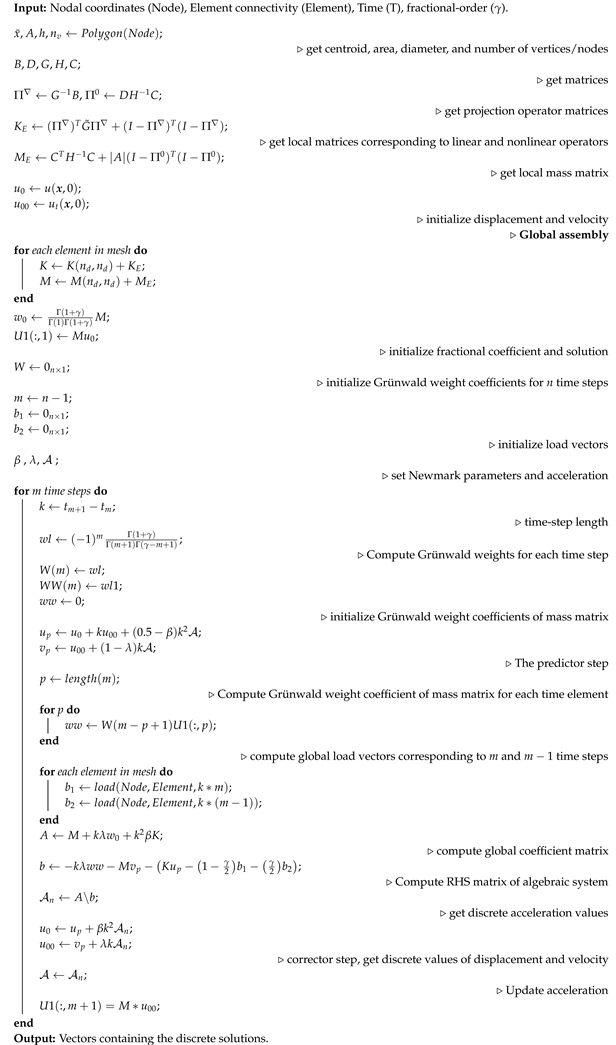
Any effective iterative technique can be used to solve the above algebraic system. It is important to note that, in the discrete formulation, the numerical solution computation at nth time step depends on the solutions that were computed at all preceding time steps, 1, 2, …, and $n-1$. The following Algorithm 1 shows the steps of implementation to solve the matrix system (41) for the resultant VEM solution. 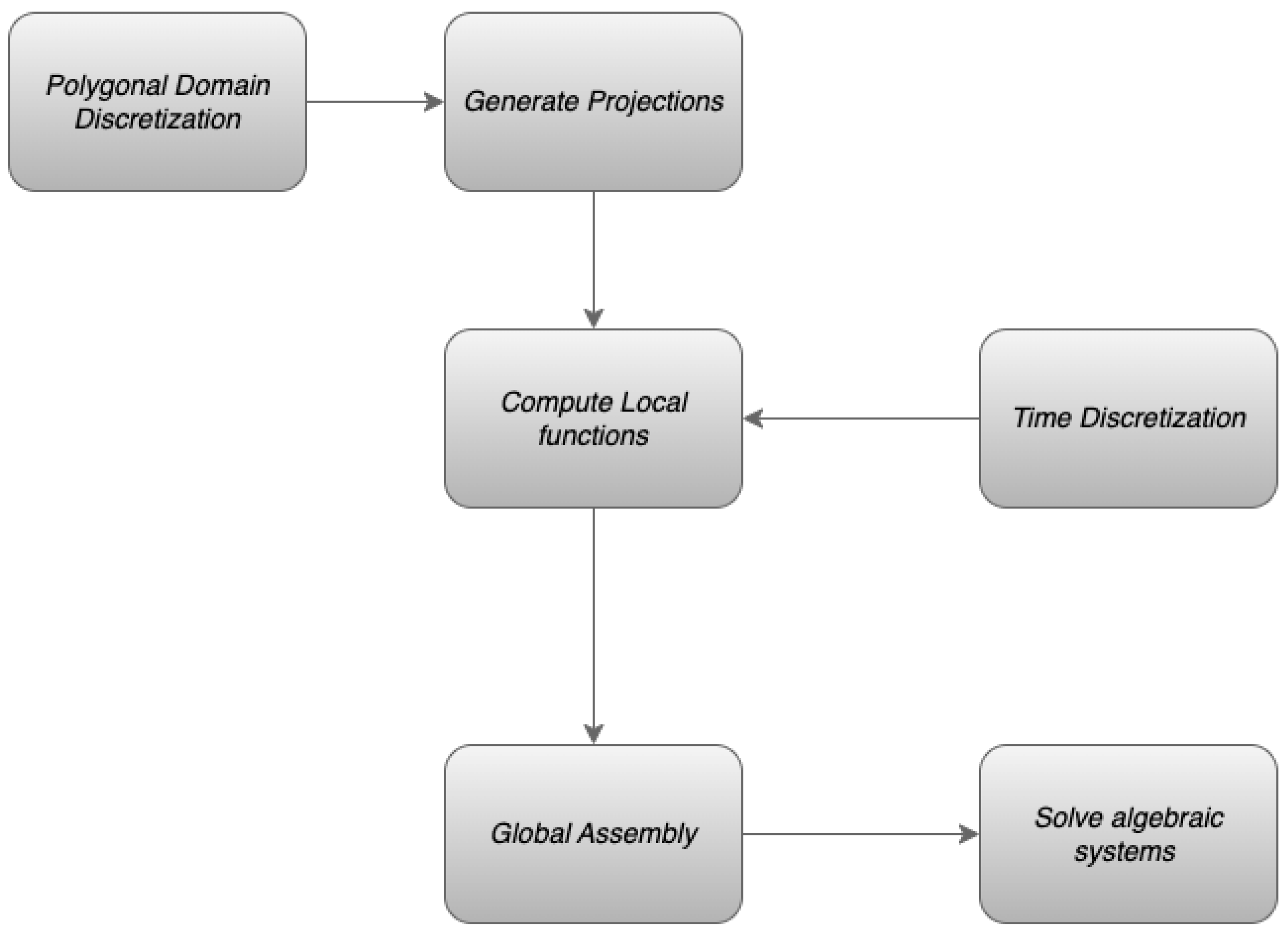For details on assembling the global matrices, refer to [21]. The schematics in Figure 2 show the implementation of the virtual element technique. Before proceeding to a detailed numerical analysis in the next section, we highlight key computational aspects of solving large-scale systems involving polygonal elements and fractional derivatives:

• The flexibility of the VEM allows for the efficient discretization of complex geometries while ensuring numerical stability through projection-based matrix assembly. However, non-triangular elements introduce increased degrees of freedom, requiring optimized assembly techniques. We adopt the methodology outlined in [21] for global assembly.
• Fractional derivatives inherently introduce long-range memory dependence, meaning that past states influence the current solution, leading to computational and storage demands. To mitigate this, many studies discuss adaptive memory truncation techniques that reduce storage requirements while preserving numerical accuracy. Furthermore, the Grünwald–Letnikov approximation is used to enhance computational efficiency in systems governed by fractional-order dynamics.

Figure 2. VEM implementation flowchart.

Figure 2. VEM implementation flowchart.

Algorithm 1: Virtual element method implementation

5. Numerical Experiments

In this section, we assess the performance of our approximation method by solving Problem (1) on two different test cases and using a sequence of refined regular Voronoi meshes and non-convex meshes on a square domain (sample mesh configurations given in Figure 3). To this end, we measure the approximation errors as the difference between the analytical solution $\psi$, the $L^2$ orthogonal projection, ${\mathsf{\Pi }}_k^{0,E}{\psi }_h$, and the elliptic projection, ${\mathsf{\Pi }}_k^{\nabla ,E}{\psi }_h$, of the virtual element approximation $u_h$ through the formulas $e_{h,0}^2={\displaystyle \sum _{E\in {\mathcal{T}}_h}}\left|\right|\psi -{\mathsf{\Pi }}_k^{0,E}{\psi }_h{\left|\right|}_E^2$ and $e_{h,1}^2={\displaystyle \sum _{E\in {\mathcal{T}}_h}}\left|\right|\nabla (\psi -{\mathsf{\Pi }}_k^{\nabla ,E}{\psi }_h){\left|\right|}_E^2$. By comparing the errors at two subsequent mesh refinements, we compute the convergence rate. From the theoretical results of Section 4, we expect to see the optimal convergence rates $e_{h,0}^2=\mathcal{O}\left(h^{k+1}\right)$ and $e_{h,1}^2=\mathcal{O}\left(h^k\right)$. It is noteworthy that this work extends the methodology to time-fractional dissipative wave equations. As there is no experimental data available for the direct comparison, the study remains self-contained, supported with rigorous theoretical analysis and two numerical illustrations that demonstrate the effectiveness of the proposed approach.

5.1.  Example 1

We consider the model problem (1) with dissipation coefficient $\nu =1$, whose analytic solution is given by

$$\begin{array}{c}\hfill \psi (\mathit{x},t)=\left(t^3\right)\sin \left(\pi x\right)\sin \left(\pi y\right).\end{array}$$

Consequently, the load function $g(\mathit{x},t)$ is

$$\begin{array}{cc}\hfill g(\mathit{x},t)& =\left(\left(6t\right)+{\displaystyle \frac{6t^{3-\gamma }}{\mathsf{\Gamma }(4-\gamma )}}+2{\pi }^2\left(t^3\right)\right)\sin \left(\pi x\right)\sin \left(\pi y\right).\hfill \end{array}$$

We have presented the $L^2$-norm and $H^1$-seminorm and the rates of convergence (RoC) for this problem using VEM of order $k=1$ and $k=2$ over a unit square domain of regular Voronoi mesh configuration in

Table 1. Example 1: $L^2\left(\mathsf{\Omega }\right)$-norm of the approximation error and RoC over regular Voronoi mesh configuration of unit square domain with mesh size $h=2^{\ell }$ for the VEM of order $k=1$.

ℓ	DoFs	$\mathit{\gamma }=0.5$		$\mathit{\gamma }=1$
		${\mathit{L}}^{\mathbf{2}}$-Norm	RoC	${\mathit{L}}^{\mathbf{2}}$-Norm	RoC
2	66	2.0637  $\times {10}^{-2}$	–	2.0629 $\times {10}^{-2}$	–
3	256	4.2976 $\times {10}^{-3}$	2.26	4.2909 $\times {10}^{-3}$	2.27
4	999	9.9783 $\times {10}^{-4}$	2.11	9.9191 $\times {10}^{-4}$	2.11
5	3998	2.2237 $\times {10}^{-4}$	2.17	2.1855 $\times {10}^{-4}$	2.18

,

Table 2. Example 1: $H^1\left(\mathsf{\Omega }\right)$-seminorm of the approximation error and RoC over regular Voronoi mesh configuration of unit square domain with mesh size $h=2^{\ell }$ for the VEM of order $k=1$.

ℓ	DoFs	$\mathit{\gamma }=0.5$		$\mathit{\gamma }=1$
		${\mathit{H}}^{\mathbf{1}}$-Seminorm	RoC	${\mathit{H}}^{\mathbf{1}}$-Seminorm	RoC
2	66	4.9999 $\times {10}^{-1}$	–	4.9999 $\times {10}^{-1}$	–
3	256	2.5121 $\times {10}^{-1}$	0.99	2.5121 $\times {10}^{-1}$	0.99
4	999	1.2602 $\times {10}^{-1}$	0.99	1.2602 $\times {10}^{-1}$	0.99
5	3998	6.2936 $\times {10}^{-2}$	1.00	6.2937 $\times {10}^{-2}$	1.00

,

Table 3. Example 1: $L^2\left(\mathsf{\Omega }\right)$-norm of the approximation error and RoC over regular Voronoi mesh configuration of the unit square domain with mesh size $h=2^{\ell }$ for the VEM of order $k=2$.

ℓ	DoFs	$\mathit{\gamma }=0.5$		$\mathit{\gamma }=1$
		${\mathit{L}}^{\mathbf{2}}$-Norm	RoC	${\mathit{L}}^{\mathbf{2}}$-Norm	RoC
2	195	1.4356 $\times {10}^{-3}$	–	1.4355 $\times {10}^{-3}$	–
3	767	1.7929 $\times {10}^{-4}$	3.00	1.7922 $\times {10}^{-4}$	3.00
4	2997	2.2428 $\times {10}^{-5}$	3.00	2.2334 $\times {10}^{-5}$	3.00
5	11995	3.2505 $\times {10}^{-6}$	2.79	2.7570 $\times {10}^{-6}$	3.01

and

Table 4. Example 1: $H^1\left(\mathsf{\Omega }\right)$-seminorm of the approximation error and RoC over regular Voronoi mesh configuration of unit square domain with mesh size $h=2^{\ell }$ for the VEM of order $k=2$.

ℓ	DoFs	$\mathit{\gamma }=0.5$		$\mathit{\gamma }=1$
		${\mathit{H}}^{\mathbf{1}}$-Seminorm	RoC	${\mathit{H}}^{\mathbf{1}}$-Seminorm	RoC
2	195	6.0800 $\times {10}^{-2}$	–	6.0800 $\times {10}^{-2}$	–
3	767	1.4798 $\times {10}^{-2}$	2.04	1.4798 $\times {10}^{-2}$	2.04
4	2997	3.6906 $\times {10}^{-3}$	2.00	3.6906 $\times {10}^{-3}$	2.00
5	11995	9.0793 $\times {10}^{-4}$	2.02	9.0790 $\times {10}^{-4}$	2.02

. Figure 4 and Figure 5 show VEM solutions obtained at different $\gamma$ values using VEM of orders $k=1,2$ respectively. Furthermore, Figure 6 and Figure 7 present the error plots and convergence rates at $\gamma =0.5,1$ values respectively, while as Figure 8 represents the distance and velocity plots against time at different $\gamma$ values.

5.2.  Example 2

We consider a 2D time-fractional dissipative wave equation involving the fractional derivative of Riemann-Liouville type, and it is given by

$$\begin{array}{c}\hfill D_t^2\psi (\mathit{x},t)+\nu {}^{R}D_t^{\gamma }\psi (\mathit{x},t)-\mathsf{\Delta }\psi (\mathit{x},t)=g(\mathit{x},t),\end{array}$$

where $\mathit{x}=(x,y)$, $\nu =1$, and $\mathsf{\Omega }$ is a two-dimensional spatial domain. From the analytic solution given by

$$\begin{array}{c}\hfill \psi (\mathit{x},t)=\sin \left(t^2\right)x(1-x)y(1-y),\end{array}$$

we find the load function $g(\mathit{x},t)$ to be

$$\begin{array}{cc}\hfill g(\mathit{x},t)& =\left(-4t^2\sin \left(t^2\right)+2\cos \left(t^2\right)+{\displaystyle \frac{2t^{2-\gamma }}{\mathsf{\Gamma }(3-\gamma )}}\sin \left(t^2+{\displaystyle \frac{\pi }{2}}\gamma \right)\right)x(1-x)y(1-y)\hfill \\ \hfill & +2\sin \left(t^2\right)\left(x(1-x)+y(1-y)\right).\hfill \end{array}$$

We have presented the $L^2$-norm and $H^1$-seminorm and the rates of convergence (RoC) for this problem over non-convex mesh configurations of unit square domain in

Table 5. Example 2: $L^2\left(\mathsf{\Omega }\right)$-norm of the approximation error and RoC over non-convex mesh configurations of unit square domain with mesh size $h=2^{\ell }$ for the VEM of order $k=1$.

ℓ	DoFs	$\mathit{\gamma }=0.5$		$\mathit{\gamma }=1$
		${\mathit{L}}^{\mathbf{2}}$-Norm	RoC	${\mathit{L}}^{\mathbf{2}}$-Norm	RoC
2	76	1.9324 $\times {10}^{-3}$	–	1.9321 $\times {10}^{-3}$	–
3	301	4.6645 $\times {10}^{-4}$	2.05	4.6609 $\times {10}^{-4}$	2.05
4	1201	1.0212 $\times {10}^{-4}$	2.19	1.0182 $\times {10}^{-4}$	2.19
5	4801	2.2125 $\times {10}^{-5}$	2.21	2.2319 $\times {10}^{-5}$	2.19

and

Table 6. Example 2: $H^1\left(\mathsf{\Omega }\right)$-seminorm of the approximation error and RoC over non-convex mesh configurations of unit square domain with mesh size $h=2^{\ell }$ for the VEM of order $k=1$.

ℓ	DoFs	$\mathit{\gamma }=0.5$		$\mathit{\gamma }=1$
		${\mathit{H}}^{\mathbf{1}}$-Seminorm	RoC	${\mathit{H}}^{\mathbf{1}}$-Seminorm	RoC
2	76	3.4607 $\times {10}^{-2}$	–	3.4607 $\times {10}^{-2}$	–
3	301	1.7484 $\times {10}^{-2}$	0.98	1.7483 $\times {10}^{-2}$	0.98
4	1201	8.7590 $\times {10}^{-3}$	0.99	8.7590 $\times {10}^{-3}$	0.99
5	4801	4.3810 $\times {10}^{-3}$	1.00	4.3811 $\times {10}^{-3}$	1.00

using the fully discrete VEM of order $k=1$ and in

Table 7. Example 2: $L^2\left(\mathsf{\Omega }\right)$-norm of the approximation error over non-convex mesh configuration of unit square domain with mesh size $h=2^{\ell }$ for the VEM of order $k=2$ at different time step sizes.

ℓ	DoFs	$\mathit{\gamma }=0.5$		$\mathit{\gamma }=1$
		$\mathit{\tau }\mathbf{=}\mathbf{1}\mathbf{/}\mathbf{50}$	$\mathit{\tau }\mathbf{=}\mathbf{1}\mathbf{/}\mathbf{100}$	$\mathit{\tau }\mathbf{=}\mathbf{1}\mathbf{/}\mathbf{50}$	$\mathit{\tau }\mathbf{=}\mathbf{1}\mathbf{/}\mathbf{100}$
2	201	1.2911 $\times {10}^{-4}$	1.2967 $\times {10}^{-4}$	1.2910 $\times {10}^{-4}$	1.2967 $\times {10}^{-4}$
3	801	1.8287 $\times {10}^{-5}$	1.6498 $\times {10}^{-5}$	1.8331 $\times {10}^{-5}$	1.6507 $\times {10}^{-5}$
4	3201	9.9562 $\times {10}^{-6}$	5.2615 $\times {10}^{-6}$	1.0044 $\times {10}^{-5}$	5.2948 $\times {10}^{-6}$
5	12,801	9.8143 $\times {10}^{-6}$	4.9339 $\times {10}^{-6}$	9.9042 $\times {10}^{-6}$	4.9700 $\times {10}^{-6}$

and

Table 8. Example 2: $H^1\left(\mathsf{\Omega }\right)$-seminorm of the approximation error over non-convex mesh configuration of unit square domain with mesh size $h=2^{\ell }$ for the VEM of order $k=2$ at different time step sizes.

ℓ	DoFs	$\mathit{\gamma }=0.5$		$\mathit{\gamma }=1$
		$\mathit{\tau }\mathbf{=}\mathbf{1}\mathbf{/}\mathbf{50}$	$\mathit{\tau }\mathbf{=}\mathbf{1}\mathbf{/}\mathbf{100}$	$\mathit{\tau }\mathbf{=}\mathbf{1}\mathbf{/}\mathbf{50}$	$\mathit{\tau }\mathbf{=}\mathbf{1}\mathbf{/}\mathbf{100}$
2	201	5.2187 $\times {10}^{-3}$	5.2189 $\times {10}^{-3}$	5.2187 $\times {10}^{-3}$	5.2190 $\times {10}^{-3}$
3	801	1.3263 $\times {10}^{-3}$	1.3258 $\times {10}^{-3}$	1.3263 $\times {10}^{-3}$	1.3258 $\times {10}^{-3}$
4	3201	3.3563 $\times {10}^{-4}$	3.3352 $\times {10}^{-4}$	3.3568 $\times {10}^{-4}$	3.3353 $\times {10}^{-4}$
5	12,801	9.4002 $\times {10}^{-5}$	8.6109 $\times {10}^{-5}$	9.4188 $\times {10}^{-5}$	8.6150 $\times {10}^{-5}$

, we present the error values at different time steps with different spatial mesh sizes using the VEM of order $k=2$. Figure 9 and Figure 10 show VEM solutions obtained at different $\gamma$ values. Furthermore, Figure 11 presents the error plots and convergence rates at $\gamma =0.5,1$ values, while as Figure 12 represents the distance and velocity plots against time at different $\gamma$ values. The results obtained provide a strong validation of the theoretical findings and provide an efficient numerical alternative with flexible tendencies for complex problems over domains with complex mesh structures.

6. Conclusions

This work has presented the formulation of a fully discrete VEM for a 2D wave equation involving a fractional-order dissipative term. The approach incorporates the Grünwald–Letnikov approximation for a time-fractional derivative of Riemann–Liouville type in conjunction with the Newmark predictor–corrector approach for the temporal domain and the VEM for spatial discretization. Theoretical results have been provided for the fully discrete scheme, including proofs of well-posedness, a priori bounds, and convergence estimates. In addition, the implementation details and an algorithm for the numerical procedure have been outlined. Numerical illustrations have been presented to validate the theoretical findings. The results obtained over two different mesh configurations is one of the many efficient advantages of using VEM for PDEs. This discrete formulation is particularly suitable for applied problems where dissipation exhibits non-ideal behavior. The immediate focus of this work has been the numerical modeling of epileptic seizures and a subject-specific studies to simulate and predict the duration of epileptic seizures, wave propagation, and identifying critical regions within the domain.

References

1. Podlubny, I. (Ed.) Fractional Differential Equations: An Introduction to Fractional Derivatives, Fractional Differential Equations, to Methods of their Solution and Some of Their Applications; Elsevier: Amsterdam, The Netherlands; Technical University of Kosice: Košice, Slovakia, 1999; Volume 198. [Google Scholar]
2. Wazwaz, A.M. Linear and Nonlinear Integral Equations: Methods and Applications, 1st ed.; Springer: Berlin/Heidelberg, Germany, 2011. [Google Scholar] [CrossRef]
3. Bandrowski, B.; Karczewska, A.; Rozmej, P. Numerical solutions to integral equations equivalent to differential equations with fractional time. Int. J. Appl. Math. Comput. Sci. 2010, 20, 261–269. [Google Scholar] [CrossRef]
4. Baeumer, B.; Kovács, M.; Sankaranarayanan, H. Higher order Grünwald approximations of fractional derivatives and fractional powers of operators. Trans. Am. Math. Soc. 2014, 367, 813–834. [Google Scholar] [CrossRef]
5. Sousa, E. Finite difference approximations for a fractional advection diffusion problem. J. Comput. Phys. 2009, 228, 4038–4054. [Google Scholar] [CrossRef]
6. Acosta, G.; Borthagaray, J. A Fractional Laplace Equation: Regularity of Solutions and Finite Element Approximations. SIAM J. Numer. Anal. 2015, 55. [Google Scholar] [CrossRef]
7. Acosta, G.; Bersetche, F.; Borthagaray, J. A short FE implementation for a 2d homogeneous Dirichlet problem of a Fractional Laplacian. Comput. Math. Appl. 2017, 74, 784–816. [Google Scholar] [CrossRef]
8. Ervin, V.; Roop, J. Variational formulation for the stationary fractional advection dispersion equation. Numer. Methods Partial. Differ. Equ. 2006, 22, 558–576. [Google Scholar] [CrossRef]
9. Esen, A.; Ucar, Y.; Yagmurlu, N.; Tasbozan, O. A Galerkin Finite Element Method to Solve Fractional Diffusion and Fractional Diffusion-Wave Equations. Math. Model. Anal. 2013, 18, 260–273. [Google Scholar] [CrossRef]
10. Jin, B.; Lazarov, R.; Zhou, Z. A Petrov-Galerkin Finite Element Method for Fractional Convection-Diffusion Equations. SIAM J. Numer. Anal. 2015, 54. [Google Scholar] [CrossRef]
11. Dar, Z.M.; Arrutselvi, M.; Chandru, M.; Manzini, G.; Natarajan, S. Analytical and Numerical Methods for Solving Fractional-Order Partial Differential Equations and the Virtual Element Method; Elsevier: Amsterdam, The Netherlands, 2024; Pre-print; Available online: https://ssrn.com/abstract=4913214 (accessed on 1 August 2024).
12. Zeghal, A. Existence result for inverse problems associated with a nonlinear parabolic equation. J. Math. Anal. Appl. 2002, 272, 240–248. [Google Scholar] [CrossRef]
13. Jin, B.; Li, B.; Zhou, Z. Numerical Analysis of Nonlinear Subdiffusion Equations. SIAM J. Numer. Anal. 2018, 56, 1–23. [Google Scholar] [CrossRef]
14. Li, D.; Wu, C.; Zhang, Z. Linearized Galerkin FEMs for Nonlinear Time Fractional Parabolic Problems with Non-smooth Solutions in Time Direction. J. Sci. Comput. 2019, 80, 1–17. [Google Scholar] [CrossRef]
15. Jin, B.; Li, B.; Zhou, Z. An analysis of the Crank-Nicolson method for subdiffusion. IMA J. Numer. Anal. 2018, 38, 518–541. [Google Scholar] [CrossRef]
16. Feng, C.H.; Tian, B.; Gao, X.T. Bilinear Bäcklund Transformations, as well as N-Soliton, Breather, Fission/Fusion and Hybrid Solutions for a (3+1)-Dimensional Integrable Wave Equation in a Fluid. Qual. Theory Dyn. Syst. 2025, 24, 100. [Google Scholar] [CrossRef]
17. Gao, X.Y. In an Ocean or a River: Bilinear Auto-Bäcklund Transformations and Similarity Reductions on an Extended Time-Dependent (3+1)-Dimensional Shallow Water Wave Equation. China Ocean. Eng. 2025, 39, 160–165. [Google Scholar] [CrossRef]
18. Gao, X.Y. Hetero-Bäcklund transformation, bilinear forms and multi-solitons for a (2+1)-dimensional generalized modified dispersive water-wave system for the shallow water. Chin. J. Phys. 2024, 92, 1233–1239. [Google Scholar] [CrossRef]
19. Beirão da Veiga, L.; Brezzi, F.; Cangiani, A.; Manzini, G.; Marini, L.D.; Russo, A. Basic principles of Virtual Element Methods. Math. Model. Methods Appl. Sci. 2012, 23, 199–214. [Google Scholar] [CrossRef]
20. Ahmad, B.; Alsaedi, A.; Brezzi, F.; Marini, L.D.; Russo, A. Equivalent projectors for virtual element methods. Comput. Math. Appl. 2013, 66, 376–391. [Google Scholar] [CrossRef]
21. Beirao da Veiga, L.; Brezzi, F.; Marini, L.D.; Russo, A. The Hitchhiker’s Guide to the Virtual Element Method. Math. Model. Methods Appl. Sci. 2014, 24, 1541–1573. [Google Scholar] [CrossRef]
22. Li, M.; Zhao, J.; Huang, C.; Shaochun, C. Conforming and nonconforming VEMs for the fourth-order reaction-subdiffusion equation: A unified framework. IMA J. Numer. Anal. 2022, 42, 2238–2300. [Google Scholar] [CrossRef]
23. Li, M.; Zhao, J.; Wang, Z.; Shaochun, C. Conservative conforming and nonconforming VEMs for fourth-order nonlinear Schrödinger equations with trapped term. J. Comput. Math. 2023, 42, 454–499. [Google Scholar] [CrossRef]
24. Zhang, Y.; Feng, M. A local projection stabilization virtual element method for the time-fractional Burgers equation with high Reynolds numbers. Appl. Math. Comput. 2023, 436, 127509. [Google Scholar] [CrossRef]
25. Zhang, Y.; Feng, M. The virtual element method for the time fractional convection diffusion reaction equation with non-smooth data. Comput. Math. Appl. 2022, 110, 1–18. [Google Scholar] [CrossRef]
26. Zhang, Y.; Feng, M. A mixed virtual element method for the time-fractional fourth-order subdiffusion equation. Numer. Algorithms 2022, 90, 1617–1637. [Google Scholar] [CrossRef]
27. Dar, Z.M.; Chandru, M. A virtual element scheme for the time-fractional parabolic PDEs over distorted polygonal meshes. Alex. Eng. J. 2024, 106, 611–619. [Google Scholar] [CrossRef]
28. Dar, Z.M.; Arrutselvi, M.; Muthusamy, C.; Natarajan, S.; Manzini, G. Virtual element approximations of the time-fractional nonlinear convection-diffusion equation on polygonal meshes. Math. Eng. 2025, 7, 96–129. [Google Scholar] [CrossRef]
29. Mascotto, L. Ill-conditioning in the virtual element method: Stabilizations and bases. Numer. Methods Partial. Differ. Equ. 2018, 34, 1258–1281. [Google Scholar] [CrossRef]
30. Qin, H.; Li, L.; Li, Y.; Chen, X. Time-Stepping Error Estimates of Linearized Grünwald-Letnikov Difference Schemes for Strongly Nonlinear Time-Fractional Parabolic Problems. Fractal Fract. 2024, 8, 390. [Google Scholar] [CrossRef]
31. Dimitrov, Y. Numerical approximations for fractional differential equations. J. Fract. Calc. Appl. 2015, 5. [Google Scholar] [CrossRef]
32. Newmark, N.M. A Method of Computation for Structural Dynamics. J. Eng. Mech. Div. 1959, 85, 67–94. [Google Scholar] [CrossRef]
33. Thomée, V. Galerkin Finite Element Method for Parabolic Problems; Springer: Berlin/Heidelberg, Germany, 2006; Volume 1054. [Google Scholar] [CrossRef]
34. Li, D.; Liao, H.l.; Sun, W.; Wang, J.; Zhang, J. Analysis of L1-Galerkin FEMs for Time-Fractional Nonlinear Parabolic Problems. Commun. Comput. Phys. 2018, 24, 86–103. [Google Scholar] [CrossRef]
35. Gorenflo, R.; Kilbas, A.A.; Mainardi, F.; Rogosin, S.V. Mittag-Leffler Functions, Related Topics and Applications; Springer: Berlin/Heidelberg, Germany, 2016. [Google Scholar] [CrossRef]
Figure 1. Degrees of freedom for VEM of orders k = 1, 2, and 3, respectively.
Fractalfract 09 00399 g001
Figure 3. Sample meshes. (a) Regular Voronoi and (b) non-convex meshes over unit square domain.
Fractalfract 09 00399 g003
Figure 4. Example 1: VEM solution over regular Voronoi mesh configuration of unit square domain at (a) γ = 0.5 and (b) γ = 1 with VEM of order k = 1 , coupled with Newmark parameters β = 0.25 and λ = 0.5 .
Fractalfract 09 00399 g004
Figure 5. Example 1: VEM solution over regular Voronoi mesh configuration of unit square domain at (a) γ = 0.5 and (b) γ = 1 with VEM of order k = 2 , coupled with Newmark parameters β = 0.25 and λ = 0.5 .
Fractalfract 09 00399 g005
Figure 6. Example 1: (a) L 2 error and (b) H 1 error plots and rate of convergence results with respect to different mesh sizes at γ = 0.5 for VEM of orders k = 1 , 2 .
Fractalfract 09 00399 g006
Figure 7. Example 1: (a) L 2 error and (b) H 1 error plots and rate of convergence results with respect to different mesh sizes at γ = 1 for VEM of orders k = 1 , 2 .
Fractalfract 09 00399 g007
Figure 8. Example 1: The displacement, velocity, and acceleration values at (a) γ = 0.5 and (b) γ = 1 over regular Voronoi meshed unit square domain for VEM of order k = 1 .
Fractalfract 09 00399 g008
Figure 9. Example 2: VEM solution over non-convex mesh configuration of unit square domain at (a) γ = 0.5 and (b) γ = 1 with VEM of order k = 1 , coupled with Newmark parameters β = 0.25 and λ = 0.5 .
Fractalfract 09 00399 g009
Figure 10. Example 2: VEM solution over non-convex mesh configuration of unit square domain at (a) γ = 0.5 and (b) γ = 1 with VEM of order k = 2 , coupled with Newmark parameters β = 0.25 and λ = 0.5 .
Fractalfract 09 00399 g010
Figure 11. Example 2: (a) L 2 error and (b) H 1 error plots and rate of convergence results with respect to different mesh sizes at γ = 0.5 , 1 for VEM of order k = 1 .
Fractalfract 09 00399 g011
Figure 12. Example 2: The displacement, velocity, and acceleration values at (a) γ = 0.5 and (b) γ = 1 over non-convex meshed unit square domain for VEM of order k = 1 .
Fractalfract 09 00399 g012