


Comparative Study of the Nonlinear Fractional Generalized Burger-Fisher Equations Using the Homotopy Perturbation Transform Method and New Iterative Transform Method


Abstract
1. Introduction
2. Basic Definitions
3. General Procedure of NITM
4. General Procedure of HPTM
5. Convergence Analysis
6. Error Estimation
7. Applications
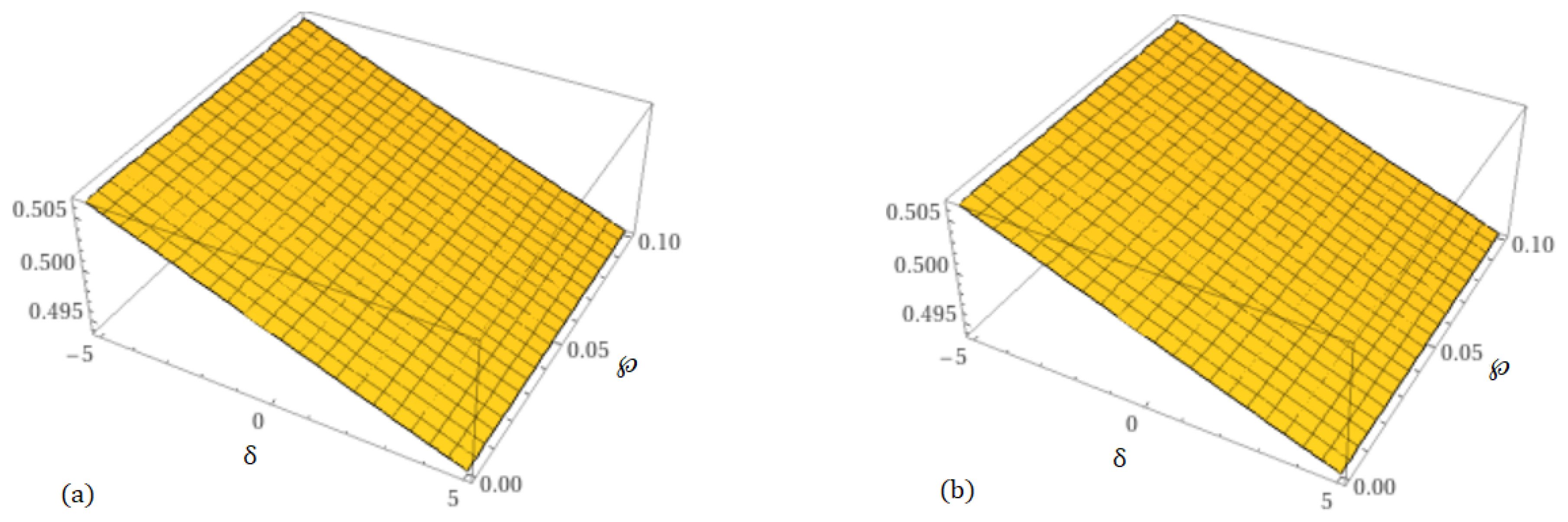
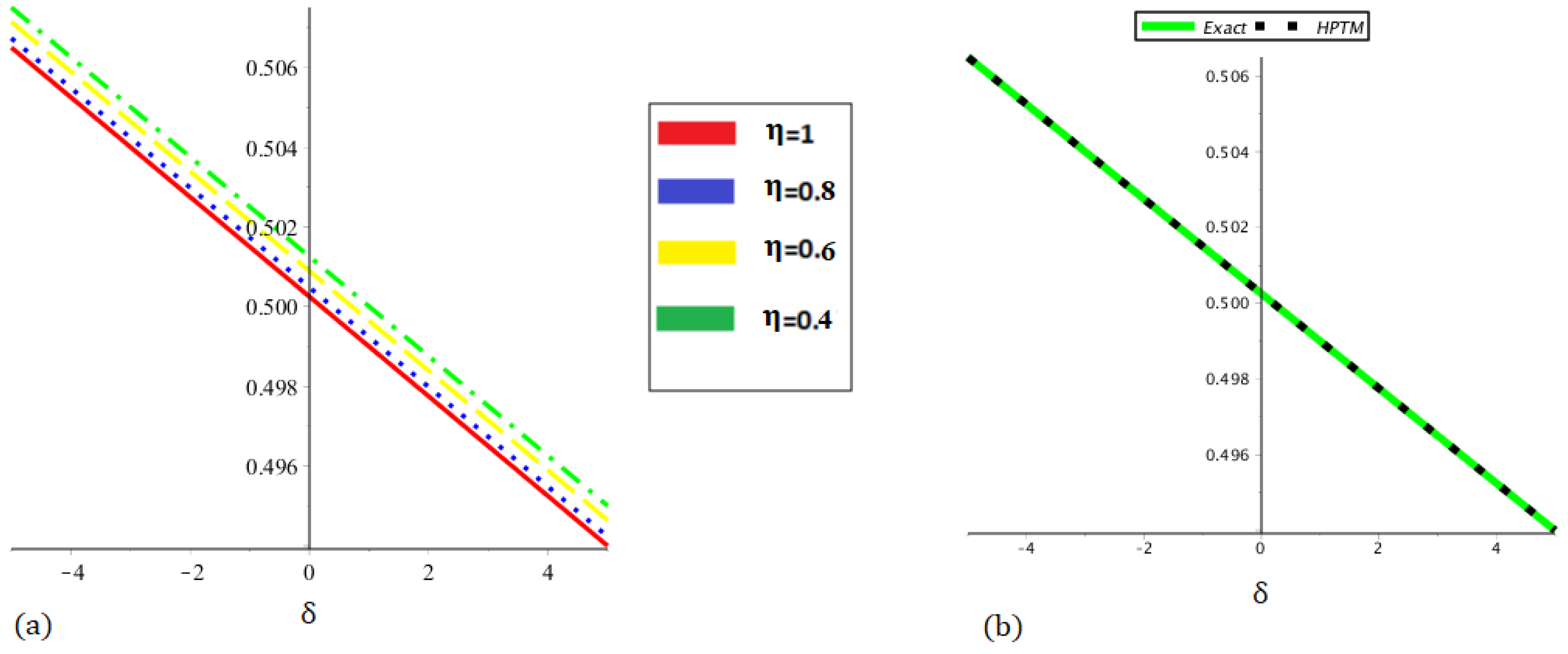
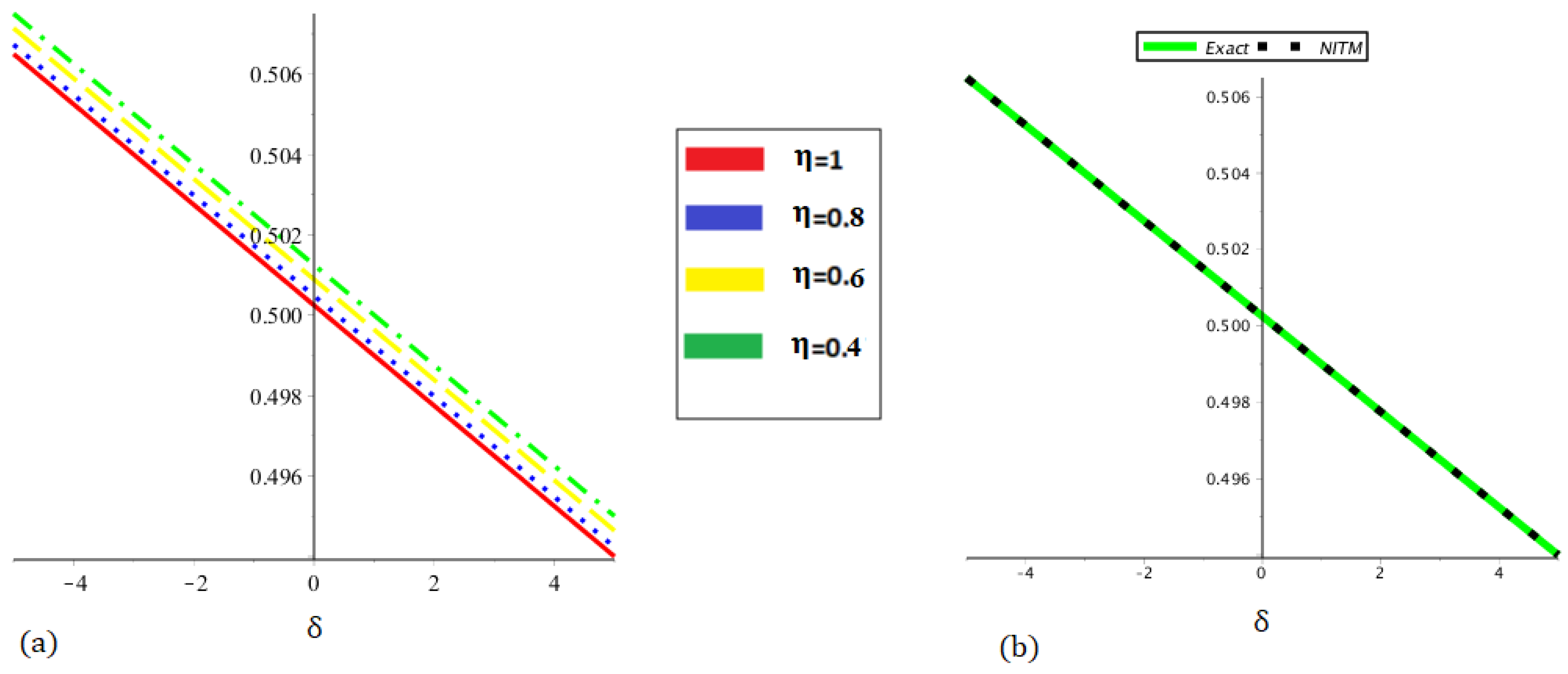
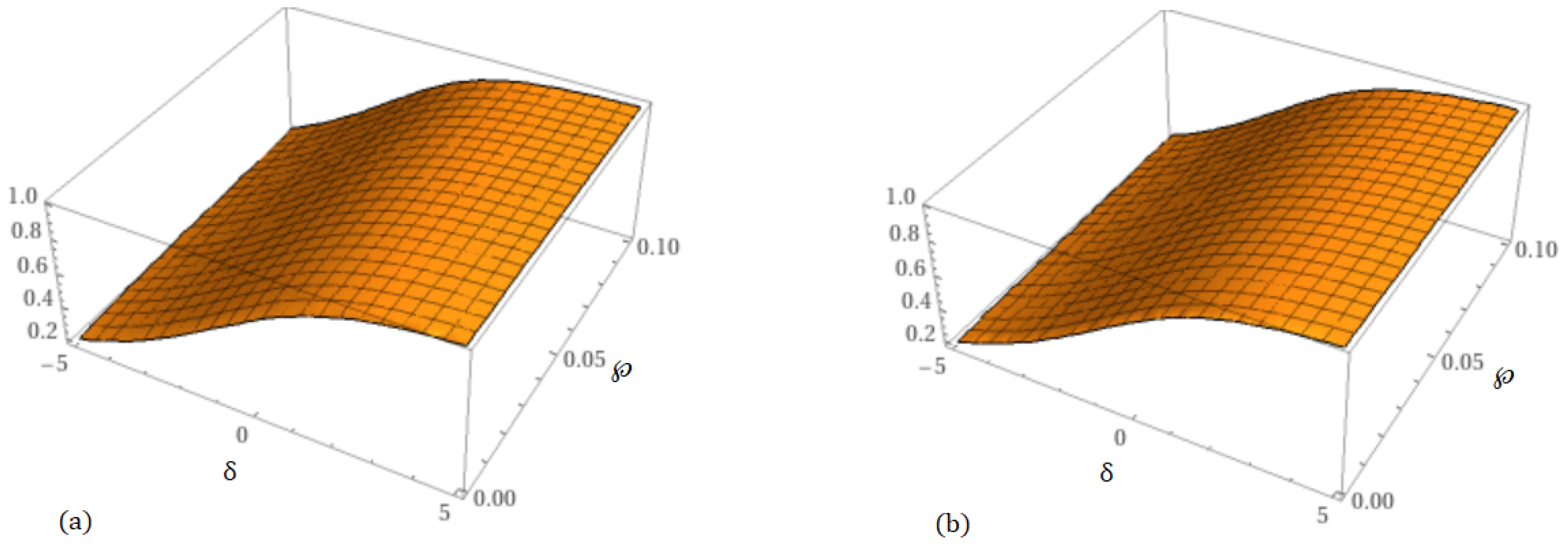
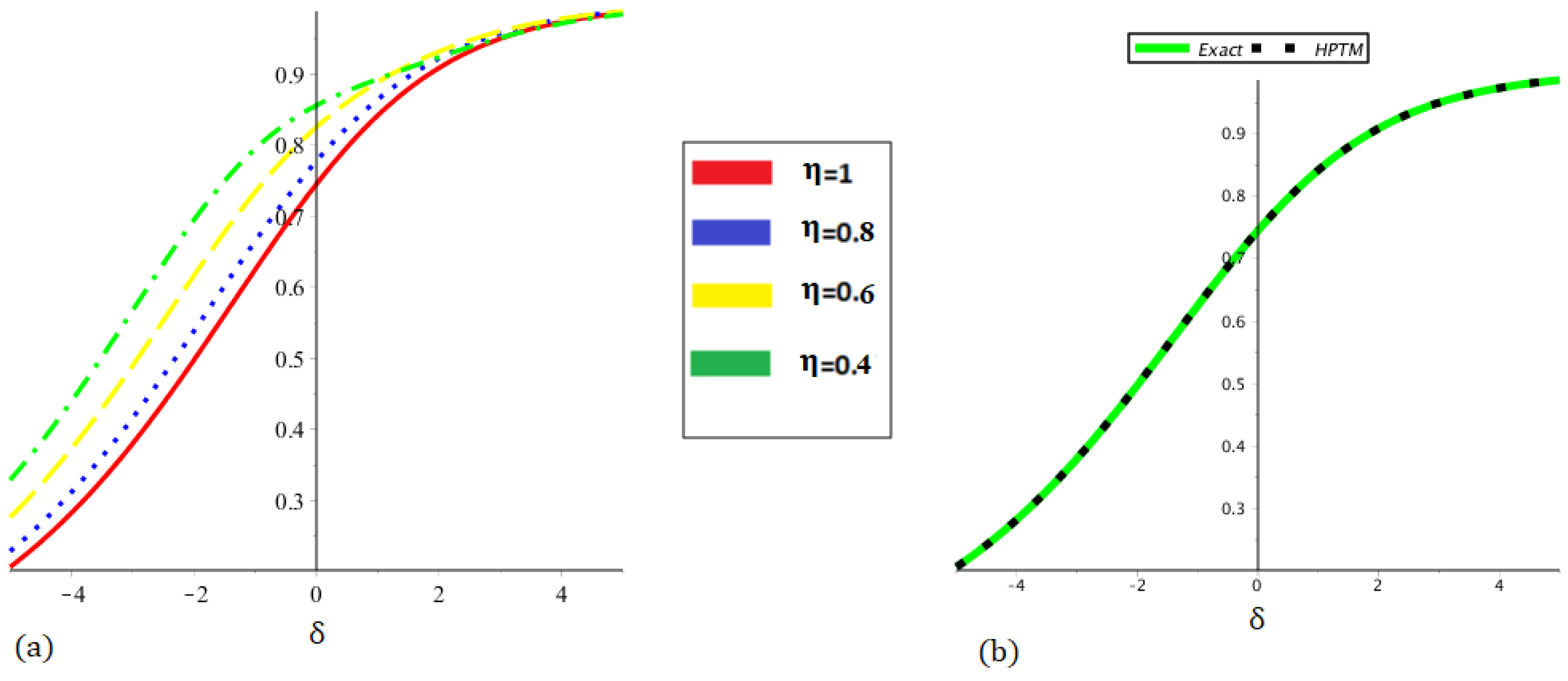
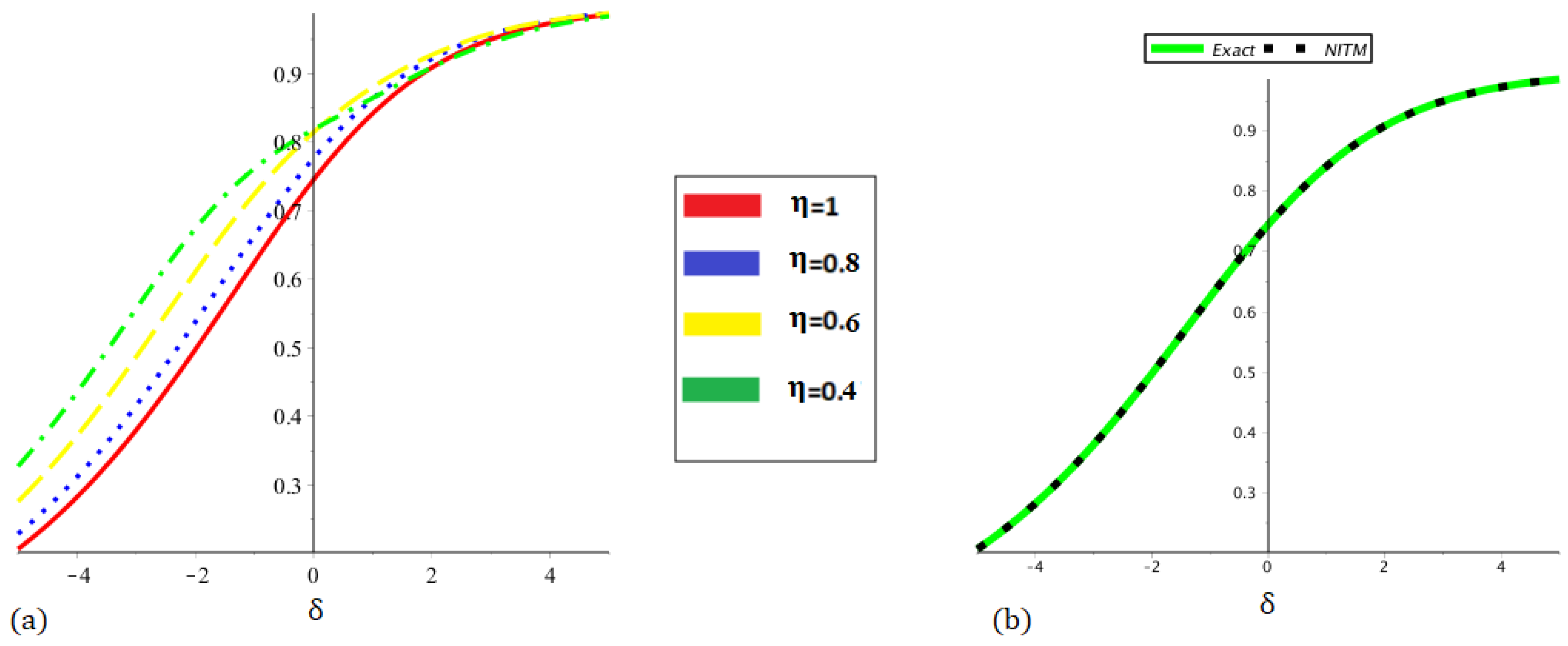
7.1. Example
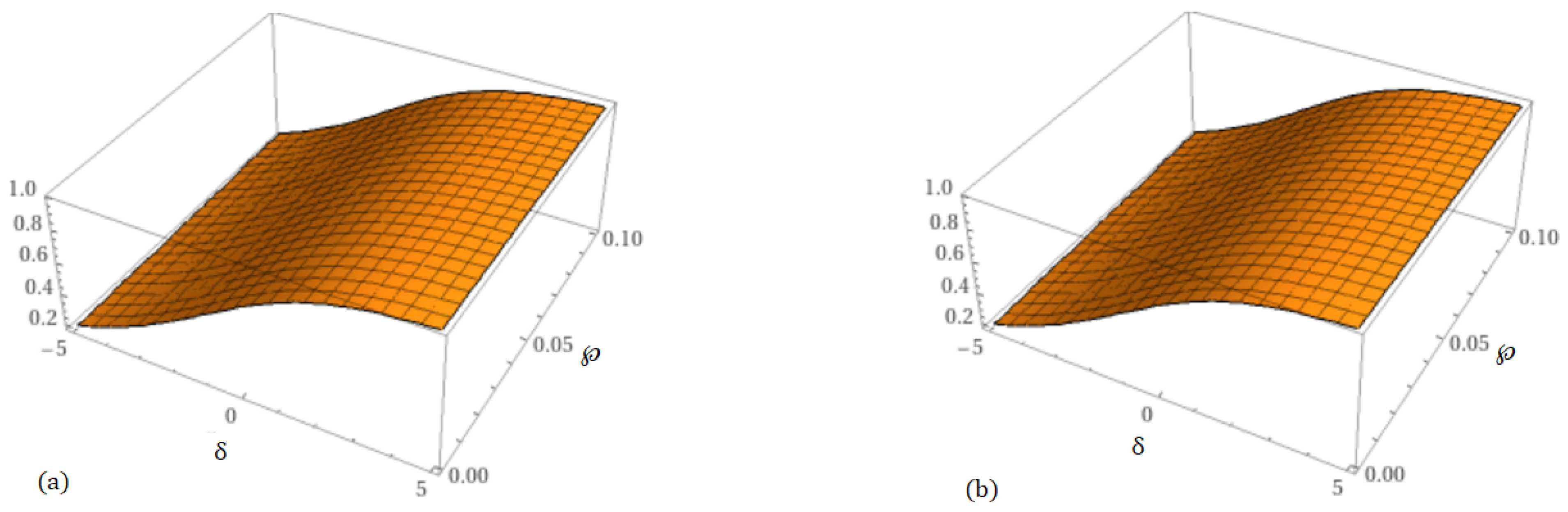
7.2. Example
8. Conclusions
Future Work
Funding
Data Availability Statement
Acknowledgments
Conflicts of Interest
Abbreviations
| TF-GBFE | time-fractional generalized Burger-Fisher equation |
| HPTM | homotopy perturbation transform method |
| YTDM | yang transform decomposition method |
| OHAM | optimal homotopy asymptotic method |
| q-HATM | q-homotopy analysis transform method |
| PDE | partial differential equation |
| FPDEs | Fractional partial differential equations |
| ET | Elzaki transform |
| Independent variable | |
| ℘ | Time |
| Dependent function representing the physical quantity | |
| Fractional order | |
| Perturbation parameter |
References
- Rezapour, S.; Liaqat, M.I.; Etemad, S. An effective new iterative method to solve conformable cauchy reaction-diffusion equation via the Shehu transform. J. Math. 2022, 12, 4172218. [Google Scholar] [CrossRef]
- Bas, E.; Ozarslan, R. Real world applications of fractional models by Atangana-Baleanu fractional derivative. Chaos Solitons Fractals 2018, 116, 121–125. [Google Scholar] [CrossRef]
- Liaqat, M.I.; Khan, A.; Akgül, A.; Ali, M. A novel numerical technique for fractional ordinary differential equations with proportional delay. J. Funct. Spaces 2022, 21, 6333084. [Google Scholar] [CrossRef]
- Traore, A.; Sene, N. Model of economic growth in the context of fractional derivative. Alex. Eng. J. 2020, 59, 4843–4850. [Google Scholar] [CrossRef]
- Khan, A.; Liaqat, M.I.; Younis, M.; Alam, A. Approximate and exact solutions to fractional order Cauchy reaction-diffusion equations by new combine techniques. J. Math. 2021, 12, 5337255. [Google Scholar] [CrossRef]
- AlBaidani, M.M.; Ganie, A.H.; Khan, A.; Aljuaydi, F. An Approximate Analytical View of Fractional Physical Models in the Frame of the Caputo Operator. Fractal Fract. 2025, 9, 199. [Google Scholar] [CrossRef]
- Shah, N.A.; El-Zahar, E.R.; Akgül, A.; Khan, A.; Kafle, J. Analysis of Fractional-Order Regularized Long-Wave Models via a Novel Transform. J. Funct. Spaces 2022, 2022, 2754507. [Google Scholar] [CrossRef]
- Hilfer, R.; Luchko, Y.; Tomovski, Z. Operational method for the solution of fractional differential equations with generalized Riemann-Liouville fractional derivatives. Fract. Calc. Appl. Anal. 2009, 12, 299–318. [Google Scholar]
- AlBaidani, M.M. Analytical Insight into Some Fractional Nonlinear Dynamical Systems Involving the Caputo Fractional Derivative Operator. Fractal Fract. 2025, 9, 320. [Google Scholar] [CrossRef]
- Ali, L.; Zou, G.; Li, N.; Mehmood, K.; Fang, P.; Khan, A. Analytical treatments of time-fractional seventh-order nonlinear equations via Elzaki transform. J. Eng. Math. 2024, 145, 1. [Google Scholar] [CrossRef]
- Jia, H.; Guo, Z.; Qi, G.; Chen, Z. Analysis of a four-wing fractional-order chaotic system via frequency-domain and time-domain approaches and circuit implementation for secure communication. Optik 2018, 155, 233–241. [Google Scholar] [CrossRef]
- He, S.; Sun, K.; Wang, H. Complexity analysis and DSP implementation of the fractional-order Lorenz hyperchaotic system. Entropy 2015, 17, 8299–8311. [Google Scholar] [CrossRef]
- Wang, Y.; Sun, K.; He, S.; Wang, H. Dynamics of fractional-order sinusoidally forced simplified Lorenz system and its synchronization. Eur. Phys. J. Spec. Top. 2014, 223, 1591–1600. [Google Scholar] [CrossRef]
- He, S.; Sun, K.; Wang, H.; Mei, X.; Sun, Y. Generalized synchronization of fractional-order hyperchaotic systems and its DSP implementation. Nonlinear Dyn. 2018, 92, 85–96. [Google Scholar] [CrossRef]
- Li, C.; Su, K.; Tong, Y.; Li, H. Robust synchronization for a class of fractional-order chaotic and hyperchaotic systems. Opt.-Int. J. Light Electron Opt. 2013, 124, 3242–3245. [Google Scholar] [CrossRef]
- Adomian, G. A review of the decomposition method and some recent results for nonlinear equations. Math. Comput. Model. 1990, 13, 17–43. [Google Scholar] [CrossRef]
- Deng, W. Short memory principle and a predictor-corrector approach for fractional differential equations. J. Comput. Appl. Math. 2007, 206, 174–188. [Google Scholar] [CrossRef]
- He, S.; Banerjee, S.; Yan, B. Chaos and symbol complexity in a conformable fractional-order memcapacitor system. Complexity 2018, 2018, 4140762. [Google Scholar] [CrossRef]
- Diethelm, K.; Ford, N.J.; Freed, A.D. A predictor-corrector approach for the numerical solution of fractional differential equations. Nonlinear Dyn. 2002, 29, 3–22. [Google Scholar] [CrossRef]
- Tavazoei, M.S.; Haeri, M. Unreliability of frequency-domain approximation in recognising chaos in fractional-order systems. IET Signal Process. 2007, 1, 171–181. [Google Scholar] [CrossRef]
- He, S.B.; Sun, K.H.; Wang, H.H. Solution of the fractional-order chaotic system based on Adomian decomposition algorithm and its complexity analysis. Acta Phys. Sin. 2014, 63, 030502. [Google Scholar]
- He, K.; Zhang, X.; Ren, S.; Sun, J. Deep residual learning for image recognition. In Proceedings of the IEEE Conference on Computer Vision and Pattern Recognition, Las Vegas, NV, USA, 27–30 June 2016; pp. 770–778. [Google Scholar]
- Wu, Z.; Shen, C.; Van Den Hengel, A. Wider or deeper: Revisiting the resnet model for visual recognition. Pattern Recognit. 2019, 90, 119–133. [Google Scholar] [CrossRef]
- Xu, W.; Fu, Y.L.; Zhu, D. ResNet and its application to medical image processing: Research progress and challenges. Comput. Methods Programs Biomed. 2023, 240, 107660. [Google Scholar] [CrossRef] [PubMed]
- Yan, H.; Du, J.; Tan, V.Y.; Feng, J. On robustness of neural ordinary differential equations. arXiv 2019, arXiv:1910.05513. [Google Scholar]
- Poli, M.; Massaroli, S.; Park, J.; Yamashita, A.; Asama, H.; Park, J. Graph neural ordinary differential equations. arXiv 2019, arXiv:1911.07532. [Google Scholar]
- Zhu, A.; Jin, P.; Zhu, B.; Tang, Y. On numerical integration in neural ordinary differential equations. In Proceedings of the International Conference on Machine Learning, Baltimore, MD, USA, 17–23 July 2022; pp. 27527–27547. [Google Scholar]
- Yang, Y.; Li, H. Neural ordinary differential equations for robust parameter estimation in dynamic systems with physical priors. Appl. Soft Comput. 2025, 169, 112649. [Google Scholar] [CrossRef]
- Yue, P. Uncertain Numbers. Mathematics 2025, 13, 496. [Google Scholar] [CrossRef]
- Yao, K.; Liu, B. Parameter estimation in uncertain differential equations. Fuzzy Optim. Decis. Mak. 2020, 19, 1–12. [Google Scholar] [CrossRef]
- Liu, Z.; Jia, L. Moment estimations for parameters in uncertain delay differential equations. J. Intell. Fuzzy Syst. 2020, 39, 841–849. [Google Scholar] [CrossRef]
- Wu, G.C.; Wei, J.L.; Luo, C.; Huang, L.L. Parameter estimation of fractional uncertain differential equations via Adams method. Nonlinear Anal. Model. Control 2022, 27, 413–427. [Google Scholar] [CrossRef]
- Ning, J.; Li, Z.; Xu, L. Parameter Estimation of Fractional Uncertain Differential Equations. Fractal Fract. 2025, 9, 138. [Google Scholar] [CrossRef]
- Rosales-García, J.; Andrade-Lucio, J.A.; Shulika, O. Conformable derivative applied to experimental Newtonas law of cooling. Rev. Mex. Fís. 2020, 66, 224–227. [Google Scholar] [CrossRef]
- Ionescu, C.; Lopes, A.; Copot, D.; Machado, J.T.; Bates, J.H. The role of fractional calculus in modeling biological phenomena: A review. Commun. Nonlinear Sci. Numer. Simul. 2017, 51, 141–159. [Google Scholar] [CrossRef]
- Rabtah, A.A.; Erturk, R.S.; Momani, S. Solution of fractional oscillator by using differential transformation method. Comput. Math. Appl. 2010, 59, 1356–1362. [Google Scholar] [CrossRef]
- Archibald, A.M.; Gusinskaia, N.V.; Hessels, J.W.; Deller, A.T.; Kaplan, D.L.; Lorimer, D.R. Universality of free fall from the orbital motion of a pulsar in a stellar triple system. Nature 2018, 559, 73–76. [Google Scholar] [CrossRef]
- Cresson, J. Fractional embedding of differential operators and Lagrangian systems. J. Math. Phys. 2007, 48, 033504. [Google Scholar] [CrossRef]
- Katugampola, U.N. A New Approach to Generalized Fractional Derivatives. arXiv 2011, arXiv:1106.0965. [Google Scholar]
- Klimek, M. Lagrangian fractional mechanics-a noncommutative approach. Czechoslov. J. Phys. 2005, 55, 1447–1453. [Google Scholar] [CrossRef]
- Ray, S.S.; Sahoo, S. New exact solutions of fractional Zakharov-Kuznetsov and modified Zakharov-Kuznetsov equations using fractional sub-equation method. Commun. Theor. Phys. 2015, 63, 25. [Google Scholar] [CrossRef]
- Gepreel, K.A.; Nofal, T.A. Optimal homotopy analysis method for nonlinear partial fractional differential equations. Math. Sci. 2015, 9, 47–55. [Google Scholar] [CrossRef]
- Khirsariya, S.R.; Chauhan, J.P.; Rao, S.B. A robust computational analysis of residual power series involving general transform to solve fractional differential equations. Math. Comput. Simul. 2024, 216, 168–186. [Google Scholar] [CrossRef]
- Zurigat, M.; Momani, S.; Odibat, Z.; Alawneh, A. The homotopy analysis method for handling systems of fractional differential equations. Appl. Math. Model. 2010, 34, 24–35. [Google Scholar] [CrossRef]
- Li, M.; Huang, C.; Wang, P. Galerkin finite element method for nonlinear fractional Schrödinger equations. Numer. Algorithms 2017, 74, 499–525. [Google Scholar] [CrossRef]
- Li, C.; Zeng, F. Finite difference methods for fractional differential equations. Int. J. Bifurc. Chaos 2012, 22, 1230014. [Google Scholar] [CrossRef]
- Kanth, A.R.; Aruna, K.; Raghavendar, K.; Rezazadeh, H.; İnç, M. Numerical solutions of nonlinear time fractional Klein-Gordon equation via natural transform decomposition method and iterative Shehu transform method. J. Ocean Eng. Sci. 2021. [Google Scholar] [CrossRef]
- Kumar, R.; Verma, R.S.; Tiwari, A.K. On similarity solutions to (2+ 1)-dispersive long-wave equations. J. Ocean Eng. Sci. 2023, 8, 11–123. [Google Scholar] [CrossRef]
- Ahmad, I.; Ahmad, H.; Inc, M.; Rezazadeh, H.; Akbar, M.A.; Khater, M.M.; Akinyemi, L.; Jhangeer, A. Solution of fractional-order Korteweg-de Vries and Burgers equations utilizing local meshless method. J. Ocean Eng. Sci. 2021. [Google Scholar] [CrossRef]
- Tang, S.; Wu, J.; Cui, M. The nonlinear convection-reaction-diffusion equation for modelling El Niño events. Commun. Nonlinear Sci. Numer. Simul. 1996, 1, 27–31. [Google Scholar] [CrossRef]
- Fakhrusy, Q.Z.; Anggraeni, C.P.; Gunawan, P.H. Simulating water and sediment flow using swe-convection diffusion model on openmp platform. In Proceedings of the 2019 7th International Conference on Information and Communication Technology (ICoICT), Kuala Lumpur, Malaysia, 24–26 July 2019; pp. 1–6. [Google Scholar]
- Khuri, S.A. A Laplace decomposition algorithm applied to a class of nonlinear differential equations. J. Appl. Math. 2001, 1, 141–155. [Google Scholar] [CrossRef]
- Khan, Y.; Wu, Q. Homotopy perturbation transform method for nonlinear equations using He’s polynomials. Comput. Math. Appl. 2011, 61, 1963–1967. [Google Scholar] [CrossRef]
- Khuri, S.A.; Sayfy, A. A Laplace variational iteration strategy for the solution of differential equations. Appl. Math. Lett. 2012, 25, 2298–2305. [Google Scholar] [CrossRef]
- Zurigat, M. Solving fractional oscillators using Laplace homotopy analysis method. Ann. Univ.-Craiova-Math. Comput. Sci. Ser. 2011, 38, 1–11. [Google Scholar]
- Guo, S.; Li, Y.; Wang, D. 2-Term Extended Rota-Baxter Pre-Lie∞-Algebra and Non-Abelian Extensions of Extended Rota-Baxter Pre-Lie Algebras. Results Math. 2025, 80, 96. [Google Scholar] [CrossRef]
- Ali, N.; Nawaz, R.; Zada, L.; Mouldi, A.; Bouzgarrou, S.M.; Sene, N. Analytical approximate solution of the fractional order biological population model by using natural transform. J. Nanomater. 2022, 2022, 6703086. [Google Scholar] [CrossRef]
- He, J.H. Homotopy perturbation technique. Comput. Methods Appl. Mech. Eng. 1999, 178, 257–262. [Google Scholar] [CrossRef]
- He, J.H. A coupling method of a homotopy technique and a perturbation technique for non-linear problems. Int. J. Non-Linear Mech. 2000, 35, 37–43. [Google Scholar] [CrossRef]
- Neamaty, A.; Agheli, B.; Darzi, R. Applications of homotopy perturbation method and Elzaki transform for solving nonlinear partial differential equations of fractional order. J. Nonlin. Evolut. Equat. Appl. 2016, 2015, 91–104. [Google Scholar]
- Podlubny, I. Fractional Differential Equations: An Introduction to Fractional Derivatives, Fractional Differential Equations, to Methods of Their Solution and Some of Their Applications; Academic Press: New York, NY, USA, 1998; 340p. [Google Scholar]
- Sedeeg, A.K.H. A coupling Elzaki transform and homotopy perturbation method for solving nonlinear fractional heat-like equations. Am. J. Math. Comput. Model. 2016, 1, 15–20. [Google Scholar]
- Bhalekar, S.; Daftardar-Gejji, V. Convergence of the new iterative method. Int. J. Differ. Equ. 2011, 2011, 989065. [Google Scholar] [CrossRef]
- Cooper, G.J. Error bounds for numerical solutions of ordinary differential equations. Numer. Math. 1971, 18, 162–170. [Google Scholar] [CrossRef]
- Warne, P.G.; Warne, D.P.; Sochacki, J.S.; Parker, G.E.; Carothers, D.C. Explicit a-priori error bounds and adaptive error control for approximation of nonlinear initial value differential systems. Comput. Math. Appl. 2006, 52, 1695–1710. [Google Scholar] [CrossRef]
- Yüzbaşi, Ş. A numerical approach for solving a class of the nonlinear Lane-Emden type equations arising in astrophysics. Math. Methods Appl. Sci. 2011, 34, 2218–2230. [Google Scholar] [CrossRef]
- Gupta, A.K.; Ray, S.S. On the Solutions of Fractional Burgers-Fisher and Generalized Fisher’s Equations Using Two Reliable Methods. Int. J. Math. Math. Sci. 2014, 2014, 682910. [Google Scholar] [CrossRef]
- Veeresha, P.; Prakasha, D.G.; Baskonus, H.M. Novel simulations to the time-fractional Fisher’s equation. Math. Sci. 2019, 13, 33–42. [Google Scholar] [CrossRef]


| 0.0 | 0.5002718980 | 0.5002646308 | 0.5002575411 | 0.5002506250 | 0.5002506250 |
| 0.1 | 0.5001468979 | 0.5001396308 | 0.5001325410 | 0.5001256250 | 0.5001256250 |
| 0.2 | 0.5000218980 | 0.5000146308 | 0.5000075411 | 0.5000006250 | 0.5000006250 |
| 0.3 | 0.4998968980 | 0.4998896309 | 0.4998825411 | 0.4998756251 | 0.4998756250 |
| 0.4 | 0.4997718981 | 0.4997646308 | 0.4997575411 | 0.4997506250 | 0.4997506250 |
| 0.5 | 0.4996468980 | 0.4996396309 | 0.4996325412 | 0.4996256251 | 0.4996256251 |
| 0.6 | 0.4995218981 | 0.4995146310 | 0.4995075413 | 0.4995006252 | 0.4995006252 |
| 0.7 | 0.4993968983 | 0.4993896312 | 0.4993825414 | 0.4993756253 | 0.4993756253 |
| 0.8 | 0.4992718985 | 0.4992646313 | 0.4992575416 | 0.4992506256 | 0.4992506256 |
| 0.9 | 0.4991468988 | 0.4991396317 | 0.4991325420 | 0.4991256259 | 0.4991256259 |
| 1.0 | 0.4990218993 | 0.4990146321 | 0.4990075424 | 0.4990006263 | 0.4990006263 |
| ℘ | Haar Wavelet Error [67] | OHAM Error [67] | q-HATM Error [68] | HPTM Error | NITM Error | |
|---|---|---|---|---|---|---|
| 0.1 | 0.2 | 5.4804 | 4.2290 | 1.1102 | 0 | 0 |
| 0.4 | 2.3476 | 8.4080 | 8.8818 | 0 | 0 | |
| 0.6 | 7.8526 | 3.4030 | 9.6589 | 0 | 0 | |
| 0.8 | 3.9181 | 8.7368 | 4.7517 | 1.0 | 1.0 | |
| 0.2 | 0.2 | 2.3553 | 8.3330 | 1.1102 | 0 | 0 |
| 0.4 | 7.7785 | 3.3840 | 4.4409 | 1.0 | 1.0 | |
| 0.6 | 3.9108 | 2.2730 | 2.7756 | 0 | 0 | |
| 0.8 | 7.0440 | 6.7268 | 2.6090 | 0 | 0 | |
| 0.3 | 0.2 | 7.0426 | 2.0890 | 1.1102 | 0 | 0 |
| 0.4 | 3.9091 | 1.6420 | 1.7764 | 0 | 0 | |
| 0.6 | 7.7594 | 1.1420 | 3.9968 | 1.0 | 1.0 | |
| 0.8 | 2.3578 | 4.7168 | 4.5519 | 1.0 | 1.0 | |
| 0.4 | 0.2 | 3.9169 | 3.3460 | 3.3307 | 0 | 0 |
| 0.4 | 7.8222 | 6.6670 | 3.3305 | 1.0 × 10⁻¹⁰ | 1.0 × 10⁻¹⁰ | |
| 0.6 | 2.3516 | 1.1300 | 1.088 | 0 | 0 | |
| 0.8 | 5.4870 | 2.7068 | 1.7097 | 0 | 0 | |
| 0.5 | 0.2 | 7.9054 | 4.6020 | 3.3307 | 1.0 | 1.0 |
| 0.4 | 2.3463 | 1.1692 | 4.5519 | 0 | 0 | |
| 0.6 | 5.4812 | 1.1190 | 1.7652 | 1.0 | 1.0 | |
| 0.8 | 8.6199 | 6.9680 | 3.8636 | 1.0 | 1.0 | |
| 0.6 | 0.2 | 5.4768 | 5.8580 | 4.9960 | 1.0 | 1.0 |
| 0.4 | 2.3384 | 1.6717 | 5.9952 | 0 | 0 | |
| 0.6 | 7.9731 | 2.2490 | 2.4536 | 1.0 | 1.0 | |
| 0.8 | 3.9384 | 1.3132 | 6.0174 | 1.0 | 1.0 | |
| 0.7 | 0.2 | 2.3489 | 7.1150 | 4.9960 | 0 | 0 |
| 0.4 | 7.9370 | 2.1742 | 7.2164 | 0 | 0 | |
| 0.6 | 3.9317 | 3.3810 | 3.1419 | 0 | 0 | |
| 0.8 | 7.0791 | 3.3232 | 8.1712 | 1.0 | 1.0 | |
| 0.8 | 0.2 | 7.0337 | 8.3710 | 6.1062 | 1.0 | 1.0 |
| 0.4 | 3.8884 | 2.6767 | 8.5487 | 0 | 0 | |
| 0.6 | 7.4894 | 4.5110 | 3.8192 | 0 | 0 | |
| 0.8 | 2.4026 | 5.3332 | 1.0325 | 1.0 | 1.0 | |
| 0.9 | 0.2 | 3.9031 | 9.6270 | 7.2164 | 0 | 0 |
| 0.4 | 7.5074 | 3.1792 | 9.9365 | 0 | 0 | |
| 0.6 | 2.3923 | 5.6420 | 4.4964 | 1.0 | 1.0 | |
| 0.8 | 5.5543 | 7.3432 | 1.2479 | 1.0 | 1.0 | |
| 1.0 | 0.2 | 8.5852 | 1.0883 | 7.7716 | 0 | 0 |
| 0.4 | 5.4286 | 3.6817 | 1.1269 | 0 | 0 | |
| 0.6 | 2.2833 | 6.7720 | 5.1736 | 0 | 0 | |
| 0.8 | 8.8514 | 9.3532 | 1.4622 | 1.0 | 1.0 |
| 0.0 | 0.7116581992 | 0.7114365594 | 0.7112253981 | 0.7110242400 | 0.7110241395 |
| 0.1 | 0.7232619661 | 0.7230443269 | 0.7228369684 | 0.7226394249 | 0.7226393305 |
| 0.2 | 0.7346476339 | 0.7344342783 | 0.7342309925 | 0.7340373213 | 0.7340372335 |
| 0.3 | 0.7458007792 | 0.7455919690 | 0.7453930058 | 0.7452034453 | 0.7452033650 |
| 0.4 | 0.7567081326 | 0.7565041070 | 0.7563096947 | 0.7561244628 | 0.7561243895 |
| 0.5 | 0.7673576479 | 0.7671586222 | 0.7669689664 | 0.7667882594 | 0.7667881945 |
| 0.6 | 0.7777385630 | 0.7775447277 | 0.7773600105 | 0.7771840022 | 0.7771839460 |
| 0.7 | 0.7878414402 | 0.7876529605 | 0.7874733396 | 0.7873021809 | 0.7873021325 |
| 0.8 | 0.7976581905 | 0.7974752057 | 0.7973008145 | 0.7971346329 | 0.7971345930 |
| 0.9 | 0.8071820859 | 0.8070047096 | 0.8068356568 | 0.8066745564 | 0.8066745250 |
| 1.0 | 0.8164077556 | 0.8162360756 | 0.8160724457 | 0.8159165074 | 0.8159164840 |
| 0.0 | 0.7116580097 | 0.7114363988 | 0.7112252619 | 0.7110241247 | 0.7110241395 |
| 0.1 | 0.7232617778 | 0.7230441673 | 0.7228368331 | 0.7226393103 | 0.7226393305 |
| 0.2 | 0.7346474475 | 0.7344341203 | 0.7342308586 | 0.7340372079 | 0.7340372335 |
| 0.3 | 0.7458005955 | 0.7455918133 | 0.7453928739 | 0.7452033335 | 0.7452033650 |
| 0.4 | 0.7567079523 | 0.7565039542 | 0.7563095652 | 0.7561243531 | 0.7561243895 |
| 0.5 | 0.7673574716 | 0.7671584728 | 0.7669688398 | 0.7667881521 | 0.7667881945 |
| 0.6 | 0.7777383914 | 0.7775445823 | 0.7773598872 | 0.7771838978 | 0.7771839460 |
| 0.7 | 0.7878412738 | 0.7876528195 | 0.7874732201 | 0.7873020797 | 0.7873021325 |
| 0.8 | 0.7976580298 | 0.7974750695 | 0.7973006991 | 0.7971345351 | 0.7971345930 |
| 0.9 | 0.8071819313 | 0.8070045785 | 0.8068355457 | 0.8066744623 | 0.8066745250 |
| 1.0 | 0.8164076073 | 0.8162359500 | 0.8160723393 | 0.8159164172 | 0.8159164840 |
Disclaimer/Publisher’s Note: The statements, opinions and data contained in all publications are solely those of the individual author(s) and contributor(s) and not of MDPI and/or the editor(s). MDPI and/or the editor(s) disclaim responsibility for any injury to people or property resulting from any ideas, methods, instructions or products referred to in the content. |
© 2025 by the author. Licensee MDPI, Basel, Switzerland. This article is an open access article distributed under the terms and conditions of the Creative Commons Attribution (CC BY) license (https://creativecommons.org/licenses/by/4.0/).
Share and Cite
AlBaidani, M.M. Comparative Study of the Nonlinear Fractional Generalized Burger-Fisher Equations Using the Homotopy Perturbation Transform Method and New Iterative Transform Method. Fractal Fract. 2025, 9, 390. https://doi.org/10.3390/fractalfract9060390
AlBaidani MM. Comparative Study of the Nonlinear Fractional Generalized Burger-Fisher Equations Using the Homotopy Perturbation Transform Method and New Iterative Transform Method. Fractal and Fractional. 2025; 9(6):390. https://doi.org/10.3390/fractalfract9060390
Chicago/Turabian StyleAlBaidani, Mashael M. 2025. "Comparative Study of the Nonlinear Fractional Generalized Burger-Fisher Equations Using the Homotopy Perturbation Transform Method and New Iterative Transform Method" Fractal and Fractional 9, no. 6: 390. https://doi.org/10.3390/fractalfract9060390
APA StyleAlBaidani, M. M. (2025). Comparative Study of the Nonlinear Fractional Generalized Burger-Fisher Equations Using the Homotopy Perturbation Transform Method and New Iterative Transform Method. Fractal and Fractional, 9(6), 390. https://doi.org/10.3390/fractalfract9060390